A physics-based model for fluvial valley width

The width of fluvial valley floors is a key parameter to quantifying the morphology of mountain regions. Valley floor width is relevant to diverse fields including sedimentology, fluvial geomorphology, and archaeology. The width of valleys has been argued to depend on climatic and tectonic conditions, on the hydraulics and hydrology of the river channel that forms the valley, and on sediment supply from valley walls. Here, we derive a physically based model that can be used to predict valley width and test it against three different datasets. The model applies to valleys that are carved by a river migrating laterally across the valley floor. We conceptualize river migration as a Poisson process, in which the river changes its direction stochastically at a mean rate determined by hydraulic boundary conditions. This approach yields a characteristic timescale for the river to cross the valley floor from one wall to the other. The valley width can then be determined by integrating the speed of migration over this timescale. For a laterally unconfined river that is not uplifting, the model predicts that the channel-belt width scales with river flow depth. Channel-belt width corresponds to the maximum width of a fluvial valley. We expand the model to include the effects of uplift and lateral sediment supply from valley walls. Both of these effects lead to a decrease in valley width in comparison to the maximum width. We identify a dimensionless number, termed the mobility–uplift number, which is the ratio between the lateral mobility of the river channel and uplift rate. The model predicts two limits: at high values of the mobility–uplift number, the valley evolves to the channel-belt width, whereas it corresponds to the channel width at low values. Between these limits, valley width is linked to the mobility–uplift number by a logarithmic function. As a consequence of the model, valley width increases with increasing drainage area, with a scaling exponent that typically has a value between 0.4 and 0.5, but can also be lower or higher. We compare the model to three independent datasets of valleys in experimental and natural uplifting landscapes and show that it closely predicts the first-order relationship between valley width and the mobility–uplift number.

1 Introduction

Many ancient civilizations developed in river valleys (Macklin and Lewin, 2015). There, fertile soil was readily available, and the river provided water, fish, and a transport route. It is a common observation that large rivers often feature broad valley floors with valley floodplains that are several times wider than the river itself (Fig. 1a). Valley floor width (valley width hereafter) is the width of the valley from foot to foot of the enclosing valley walls and hence the sum of river width and floodplain width. In fluvial valleys, valley width usually corresponds to the part of the valley in which the river is active on timescales encompassing multiple floods and is thus intimately related to the width of the channel belt in an unconfined setting without valley walls (Fig. 1b) (e.g. Limaye, 2020; Tofelde et al., 2022). Nearly planar valley floors not only provide space for settlements and farming, but also accommodate alluvial sediments supplied from upstream mountain regions and often host unique ecological communities. As such, valley width has been recognized as an important parameter in the development of human settlements (e.g. Hillier et al., 2007; Macklin et al., 2015; Rigsby et al., 2003), the evolution of orogenic landscapes (e.g. Hancock and Anderson, 2002; Langston and Tucker, 2018), the distribution and cycling of sediments and nutrients in the landscape (e.g. Blöthe et al., 2014; Blum and Törnqvist, 2000; Jonell et al., 2018; Repasch et al., 2021), the development of river patterns and fluvial landforms (e.g. Fotherby, 2009; Grant and Swanson, 1995; Schumm and Lichty, 1963), hydrology and flood dynamics (e.g. Appledorn et al., 2019; Miller, 1995), floodplain ecology (e.g. Baker and Wiley, 2009; Hupp, 1982; Naiman et al., 2010), speciation and biodiversity (e.g. Perrigo et al., 2020; Steinbauer et al., 2016), and the establishment of fisheries (e.g. Maasri et al., 2021; May et al., 2013).

Multiple parameters have been suggested to control valley width. It has been observed that valley width is correlated with water discharge, stream length, or drainage area, as well as upstream sediment supply in natural river valleys (e.g. Constantine et al., 2014; Dunne et al., 2010; Salisbury, 1980; Salisbury et al., 1968; Tomkin et al., 2003; Zavala et al., 2021) and analogue experiments (e.g. Bufe et al., 2016a; Martin et al., 2011). Valley width typically scales with discharge or drainage area according to a power law, with scaling exponents that vary between about 0.1 and 1.2 (e.g. Beeson et al., 2018; Brocard and van der Beek, 2006; Langston and Temme, 2019; Snyder et al., 2003; Som et al., 2009; Tomkin et al., 2003). It has also been observed that valley width is inversely correlated with uplift rate (e.g. Bufe et al., 2016a; Clubb et al., 2023a) and, in the special case of paired alluvial river terrace sequences, inversely correlated with valley wall height (Tofelde et al., 2022). In addition, for comparable discharge conditions, valleys sometimes seem to be wider in softer lithologies compared to harder lithologies (e.g. Brocard and van der Beek, 2006; Bursztyn et al., 2015; Keen-Zebert et al., 2017; Langston and Temme, 2019; Moore, 1926; Schanz and Montgomery, 2016), and widening rates have been suggested to depend on rock type and weathering (e.g. Johnson and Finnegan, 2015; Limaye and Lamb, 2014; Marcotte et al., 2021; Montgomery, 2004; Snyder and Kammer, 2008; Suzuki, 1982). Lifton et al. (2009) found a negative correlation between local valley width and the rock strength on the weaker side of the valley. In contrast, in a regional study of the Himalaya, Clubb et al. (2023a) reported that valley width is independent of lithology and concluded that uplift provides the dominant control.

Multiple authors have suggested that valley widening occurs during times when the river aggrades or moves laterally through a thick sediment fill without major incision (e.g. Maddy et al., 2001; Hancock and Anderson, 2002). Further, it has been argued that river valleys widen by lateral erosion of streams and by fluvial undercutting of valley wall hillslopes and their subsequent collapse (Brocard and van der Beek, 2006; Hancock and Anderson, 2002; Martin et al., 2011; Malatesta et al., 2017; Suzuki, 1982). In this case, widening rates decrease with increasing valley width because the river spends a decreasing fraction of time in contact with the valley walls (Hancock and Anderson, 2002; Tofelde et al., 2022). However, a steady state is never reached and the valley widens indefinitely. As a result, valley width would be determined by the time since the onset of lateral migration and erosion, as well as the widening rate. Some river valleys show paired terrace sequences, which have frequently been suggested to form in response to cyclic climate change (e.g. Bridgland and Westaway, 2008; Maddy et al., 2001; Schanz et al., 2018). Their presence implies that valleys can evolve to different widths under similar climatic conditions. To explain the occurrence of paired terraces, Tofelde et al. (2022) argued that a parameter independent of river dynamics is also important in controlling the width to which valleys evolve. They suggested that a steady-state valley width is achieved when lateral sediment supply from hillslopes is balanced with the ability of the river to remove this sediment. Their model can explain the existence of paired terrace sequences and predicts the observed inverse linear scaling between the width and total height of enclosing valley walls. Yet, the model does not predict how valley width is modulated by uplift, and it can only predict valley width in relation to a maximum valley width that is an input parameter in the equations. Tofelde et al. (2022) suggested that this maximum valley width corresponds to channel-belt width in an unconfined setting. Limaye (2020) postulated that channel-belt width scales with the channel width of the forming river, which still lacks a mechanistic explanation.

It seems clear that hydraulics and river processes (e.g. Martin et al., 2011; Suzuki, 1982) as well as tectonics (e.g. Bufe et al., 2016a; Clubb et al., 2023a) influence the width of fluvial valleys, while the role of lithology is unclear (see Clubb et al., 2023a; Langston and Temme, 2019; Lifton et al., 2009). Yet, a full understanding of the controls and a model that allows predicting valley width from known boundary conditions are currently missing. In particular, it is not understood how the observed scaling relationships between valley width, drainage area, and uplift rate arise (e.g. Beeson et al., 2018; Bufe et al., 2016a; Clubb et al., 2023a; Langston and Temme, 2019). Here, we build on previous work of Bufe et al. (2019) and Tofelde et al. (2022) and develop a physics-based model for the steady-state width of channel belts and fluvial valleys. The model predicts the width of channel belts in laterally unconfined settings and how this width is reduced in laterally confined valleys and in uplifting regions. We compare the model to three complementary datasets of rivers crossing uplifting folds in an experiment (Bufe et al., 2016a) and the Tian Shan mountain range, as well as to a valley width compilation with more than 1.6 million data points from the Himalaya (Clubb et al., 2023a, b).

2 Model development

2.1 Conceptual framework of model

We start by considering the width W [L] of a valley containing an alluvial river (Fig. 1c). We will proceed with the derivation and make a connection to bedrock river valleys in the discussion. We assume that depositional systems do not naturally lead to incised valleys. We will thus consider graded or incising channels and assume that they move laterally by bank erosion rather than avulsion. We postulate that the walls of fluvial valleys are pushed back by fluvial undercutting that drives wall collapse and subsequent evacuation of the resulting sediment when the river is located at the valley wall and moves into it (see Hancock and Anderson, 2002; Martin et al., 2011; Malatesta et al., 2017). We assume that processes acting in the long-channel direction are negligible to first order and that each point of the river can be treated as independent of events upstream and downstream. Thus, we consider a valley cross-section, in which a stream migrates back and forth across the valley floor with lateral speed V [L T⁻¹] (Fig. 1). For a given set of climatic, tectonic, and sedimentological boundary conditions, we conceptualize the lateral motion of the channel as a stochastic process, in which switches in the direction of motion are considered identically distributed and independent stochastic events occurring at a constant mean rate. As such, the likelihood of the switches in direction have no history dependence. The stated conditions mean that the switching of directions is described by a Poisson process with rate parameter λ [T⁻¹] that quantifies the mean number of switch events per unit time. At the valley walls, the need to erode and transport sediments supplied from valley wall hillslopes may slow down the lateral speed of the channel to a value v<V (Tofelde et al., 2022). The valley width is then determined by (i) the speed of lateral migration of the river across the floodplain, (ii) the length of time the river moves on average in the same direction, and (iii) the amount of laterally supplied sediment from hillslopes (Tofelde et al., 2022). For negligible lateral sediment supply, the width W of the valley can be obtained by integrating over the product of the lateral speed of motion V and a characteristic timescale Δt [T].

$$\begin{array}{}\text{(1)}& W={\int }_{\mathrm{0}}^{\mathrm{\Delta }t}V\mathrm{d}t+W_{\mathrm{C}}\end{array}$$

The width of the river, W_C [L], needs to be added, as it presents the starting condition before any bevelling takes place. Thus, channel width W_C provides a minimum width for the valley. Equation (1) is a general formulation for valley formation by fluvial bevelling, which allows, for example, for variable V. For constant V, W = VΔt + W_C. Under the assumption that the channel switches direction of migration according to a Poisson process, the timescale Δt is related to the mean waiting time between switch events. In a Poisson process with rate constant λ, the waiting times are exponentially distributed with a mean of $\mathrm{1}/\mathit{\lambda }$. Because the process is stochastic, there is a non-negligible probability that the waiting time is larger than the average. As such, the valley sets its width to some effective lateral migration time that can be expected to scale with the mean waiting time but is not necessarily exactly equal to it. Therefore, Δt is inversely related to λ by

$$\begin{array}{}\text{(2)}& \mathrm{\Delta }t={\displaystyle \frac{c}{\mathit{\lambda }}},\end{array}$$

where c [−] is a dimensionless constant of order 1. We proceed by considering the average behaviour of the channel belt, essentially making the assumption that the channel switches direction of migration at regular intervals Δt. Then, the equations yield a well-defined steady state and spatially stable channel belt. In a fully stochastic model, the channel belt would drift laterally once it reaches the steady-state width.

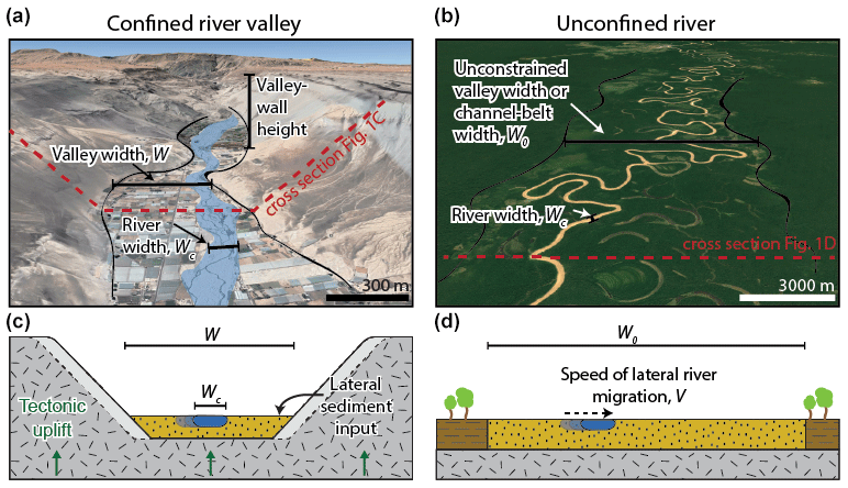
Figure 1 Examples and concepts for confined river valleys and unconfined rivers. (a) Oblique view from © Google Earth of the San Jose River, Chile (18.58° S, 69.97° W), showing a confined valley. Debris cones on the valley flanks are signs for substantial sediment input from valley walls into the river valley. The scale bars refer to the foreground. (b) Oblique view from © Google Earth of the Juruá River, Brazil (6.75° S, 70.30° W), that is laterally unconfined. (c) Conceptual sketch of the dynamics in a confined river valley. (d) Conceptual sketch for the dynamics in an unconfined channel belt.

2.2 Model derivation

2.2.1 Unconfined river: channel-belt width

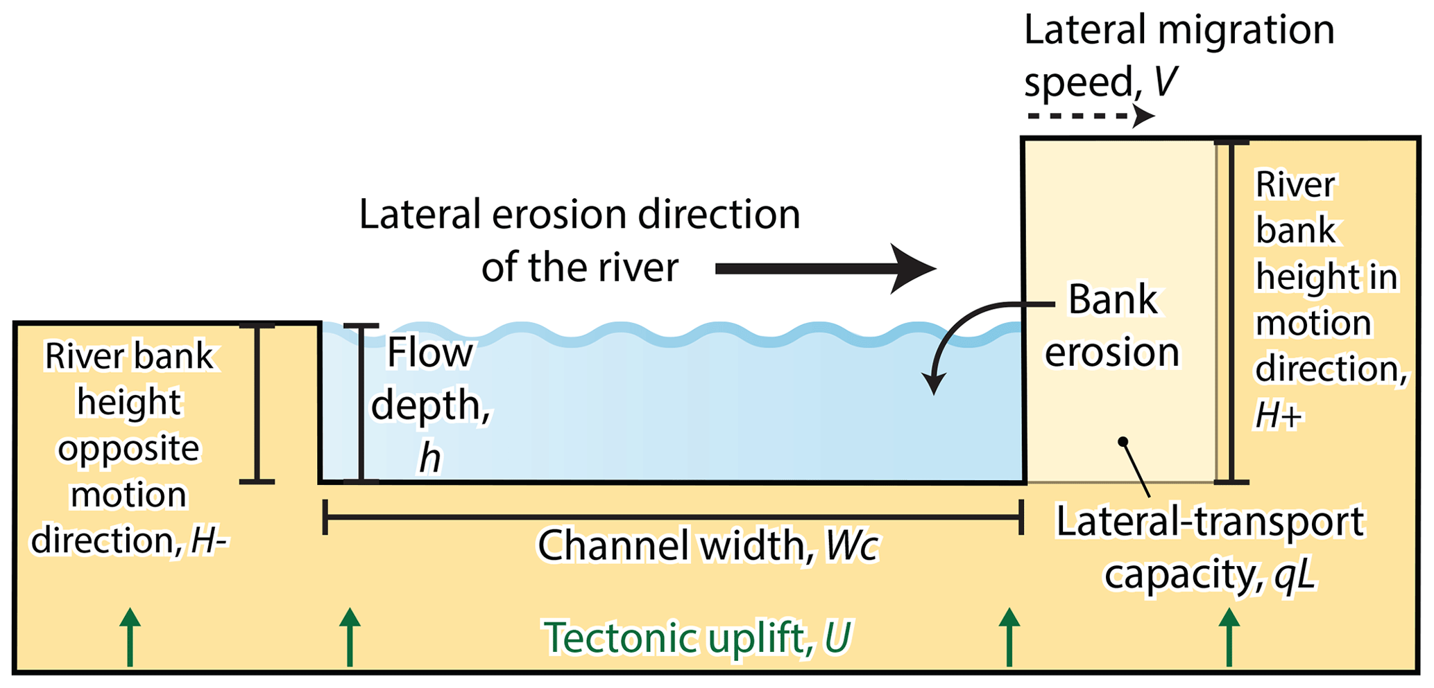
To complete the model, we need to provide equations for the channel's lateral speed of migration V and the rate parameter λ, which we will treat in turn. For the former, we use the concept of Bufe et al. (2019) that states that, for a given discharge, sediment supply, and grain size, the amount of sediment that the channel can move by lateral erosion per unit channel length per unit time is constant and can be expressed by a lateral transport capacity q_L [L² T⁻¹] (Fig. 2). The lateral migration speed, V, is then equal to the ratio of q_L and the height of the riverbank in the direction of motion, H₊ [L] (Bufe et al., 2019):

$$\begin{array}{}\text{(3)}& V={\displaystyle \frac{q_{\mathrm{L}}}{H_{+}}}.\end{array}$$

Figure 2 Schematic cross-section of a migrating channel with a definition of parameters.

Both V and q_L are determined by hydraulic and sedimentological boundary conditions. The precise controls have not yet been completely resolved (e.g. Bufe et al., 2019; Constantine et al., 2014; Ielpi and Lapôtre, 2019; Wickert et al., 2013) but are not directly relevant for the remainder of the derivation. For constant boundary conditions without uplift, H₊ can be considered a constant H₀ [L], which should be equal to flow depth h [L] because during migration, the channel cannot deposit sediment at elevations higher than its flow depth. Then, Eq. (1) can be solved and the width of the channel belt in an unconfined plain, W₀, is given by

$$\begin{array}{}\text{(4)}& \begin{array}{rl}{W}_{\mathrm{0}}& ={\int }_{\mathrm{0}}^{\mathrm{\Delta }t}V\mathrm{d}t+W_{\mathrm{C}}=V\mathrm{\Delta }t+W_{\mathrm{C}}={\displaystyle \frac{q_{\mathrm{L}}}{H_{\mathrm{0}}}}\mathrm{\Delta }t\\ & +W_{\mathrm{C}}={\displaystyle \frac{c}{\mathit{\lambda }}}{\displaystyle \frac{q_{\mathrm{L}}}{h}}+W_{\mathrm{C}}.\end{array}\end{array}$$

To quantify the rate parameter λ, we postulate that the channel switches direction when its cross-section is overwhelmed by sediment derived from erosion of the bank in the migration direction, leading to water overflow of the bank opposite of the motion direction (Fig. 2). We did not find documented observations of this notion, and a thorough investigation will need to be done in the future. Yet, it is commonly observed that lateral sediment input by landslides or tributaries pushes rivers towards the opposite bank (e.g. Cruden et al., 1997; Grant and Swanson, 1995; McClain et al., 2020; Savi et al., 2020). As such, the likelihood of channel switching, λ, is proportional to the ratio of the average sediment input rate due to lateral migration, q_L (yellow shaded area in Fig. 2), and the dimensions of the channel given by the product of channel width and flow depth, W_Ch (blue shaded area in Fig. 2). Thus, we suggest that λ scales as

$$\begin{array}{}\text{(5)}& \mathit{\lambda }\propto {\displaystyle \frac{q_{\mathrm{L}}}{W_{\mathrm{C}}h}}.\end{array}$$

However, Eq. (5) is not a complete description of the scaling. We expect that λ depends not only on the sediment input rate relative to the channel cross-sectional area, but also on the aspect ratio of the channel. In particular, we suggest that deep and narrow channels are less likely to switch directions than wide and shallow channels for otherwise similar conditions. Wide and shallow channels have a lower bank relative to the channel dimensions and lateral transport capacity, which should make switching directions more likely. Therefore, we expect that λ scales with the aspect ratio as

$$\begin{array}{}\text{(6)}& \mathit{\lambda }\sim {\displaystyle \frac{W_{\mathrm{C}}}{h}}.\end{array}$$

Multiplying Eqs. (5) and (6) gives the final relation for the rate parameter λ:

$$\begin{array}{}\text{(7)}& \mathit{\lambda }=k{\displaystyle \frac{q_{\mathrm{L}}}{h^{\mathrm{2}}}}.\end{array}$$

Here, k [−] is a dimensionless constant. Substituting Eq. (7) into Eq. (4) yields the channel-belt width in unconfined settings.

$$\begin{array}{}\text{(8)}& W_{\mathrm{0}}={\displaystyle \frac{k_{\mathrm{0}}}{H_{\mathrm{0}}}}{h}^{\mathrm{2}}+W_{\mathrm{C}}=k_{\mathrm{0}}h+W_{\mathrm{C}}\end{array}$$

Here, k₀ = $c/k$ [−] is a dimensionless constant, and we assumed H₀ = h in the latter identity. The channel-belt width W₀ predicted by Eq. (8) at the same time gives the maximum valley width in the absence of uplift and lateral hillslope sediment supply.

2.2.2 Confined valleys in uplifted regions

Here, we consider a river incising at a constant rate. The incision may be driven by relative uplift, a change in water and sediment discharge, or autogenic variations in river dynamics. We proceed with the derivation considering the case of uniform uplift, noting that the results should be equivalent for any other process driving river incision.

In an uplifted region, the river adjusts to a state in which the incision rate equals the uplift rate (e.g. Howard, 1994; Turowski, 2020). Yet, the parts of the valley floor where the channel is not currently located rise in elevation at the uplift rate U [L T⁻¹]. As the river migrates laterally, it therefore needs to remove the additional sediment material provided due to uplift. The amount of this sediment at a particular location scales with the product of the uplift rate and the time since the last visit of the river at that location. We can model this as an increase in the bank height H₊ encountered by the river, which is given by

$$\begin{array}{}\text{(9)}& {\displaystyle \frac{\mathrm{d}{H}_{+}}{\mathrm{d}t}}=U.\end{array}$$

Within the integral (Eq. 1), we thus need to treat H₊ as a time-dependent parameter. The integral can be solved by a substitution of variables to yield valley width W:

$$\begin{array}{}\text{(10)}& \begin{array}{rl}W& ={\int }_{\mathrm{0}}^{\mathrm{\Delta }t}{\displaystyle \frac{q_{\mathrm{L}}}{H_{+}\left(t\right)}}\mathrm{d}t+W_{\mathrm{C}}={\int }_{H_{\mathrm{0}}}^{H_{\mathrm{0}}+\mathrm{2}U\mathrm{\Delta }t}{\displaystyle \frac{q_{\mathrm{L}}}{U{H}_{+}}}\mathrm{d}{H}_{+}+W_{\mathrm{C}}\\ & ={\displaystyle \frac{q_{\mathrm{L}}}{U}}\ln \left\{\mathrm{1}+{\displaystyle \frac{\mathrm{2}U\mathrm{\Delta }t}{H_{\mathrm{0}}}}\right\}+W_{\mathrm{C}}.\end{array}\end{array}$$

Here, ln{x} denotes the natural logarithm of x. The factor of 2 in the upper limit of the integral arises because the river needs to switch direction and traverse the valley twice before arriving at the same position again. Therefore, the time elapsed between revisiting a valley margin is 2Δt. Assuming that the river cross-sectional shape is unaffected by uplift, the timescale Δt is the same as in the unconfined case (see Eqs. 2 and 7). As noted above, for consistency, we need to substitute 2Δt. Then, using Eqs. (7) and (8), W is given by

$$\begin{array}{}\text{(11)}& W={\displaystyle \frac{q_{\mathrm{L}}}{U}}\ln \left\{\mathrm{1}+{\displaystyle \frac{U\left(W_{\mathrm{0}}-W_{\mathrm{C}}\right)}{q_{\mathrm{L}}}}\right\}+W_{\mathrm{C}}.\end{array}$$

For U = 0, Eq. (11) reduces to W = W₀, as required, and for large U, W = W_C, as can be expected for entrenched rivers in rapidly uplifting landscapes.

2.2.3 Sediment supply from valley walls

To explain the geometry of paired river terraces, Tofelde et al. (2022) suggested that lateral sediment supply from hillslope erosion or back-weathering processes leads to valley narrowing because a river can only widen the valley further once this additional material deposited in sediment cones at the wall toe is evacuated. Tofelde et al. (2022) proposed that valleys reach a steady-state width, at which lateral sediment removal by the river equals lateral sediment input from hillslopes. This lateral mass balance can be written as

$$\begin{array}{}\text{(12)}& P{q}_{\mathrm{L}}=q_{\mathrm{H}}.\end{array}$$

Here, P [−] is a dimensionless parameter denoting the fraction of time that the river spends at the valley walls with a direction of motion into them, and q_H [L² T⁻¹] is the rate of sediment supply from the valley walls per unit channel length. In their proposed valley width model, Tofelde et al. (2022) derived P under the assumption that the channel width is much smaller than the valley width and can therefore be neglected. Including channel width in the derivation of P yields (compare to Eqs. 10 to 14 of Tofelde et al., 2022)

$$\begin{array}{}\text{(13)}& P={\displaystyle \frac{W_{\mathrm{0}}-W}{W_{\mathrm{0}}-W_{\mathrm{C}}}}.\end{array}$$

After substituting Eq. (13) into Eq. (12) and solving for W, valley width is given by

$$\begin{array}{}\text{(14)}& W=W_{\mathrm{0}}-{\displaystyle \frac{q_{\mathrm{H}}}{q_{\mathrm{L}}}}\left(W_{\mathrm{0}}-W_{\mathrm{C}}\right).\end{array}$$

Note that this equation is defined only as long as q_H<q_L. If lateral sediment supply exceeds the capacity of the river to transport the sediment, the river will either aggrade and steepen to increase q_L or change course and abandon the valley (Humphrey and Konrad, 2000). Equation (14) updates the model of Tofelde et al. (2022) to include a finite channel width but excludes uplift. In an uplifting region, W₀ in Eq. (14) can be identified with the width of an uplifting valley, and after substituting Eq. (11), we obtain an equation for valley width including both uplift and lateral sediment supply:

$$\begin{array}{}\text{(15)}& W=\left({\displaystyle \frac{q_{\mathrm{L}}-q_{\mathrm{H}}}{U}}\right)\ln \left\{\mathrm{1}+{\displaystyle \frac{U\left(W_{\mathrm{0}}-W_{\mathrm{C}}\right)}{q_{\mathrm{L}}}}\right\}+W_{\mathrm{C}}.\end{array}$$

For U = 0, Eq. (15) reduces to Eq. (14), and for large U, W₀ = W_C.

We can formulate a nondimensional version of Eq. (15), including four nondimensional parameters: valley width normalized to the unconfined channel-belt width $W^{\prime }=W/W_{\mathrm{0}}$, channel width normalized to the unconfined channel-belt width $W_{\mathrm{C}}^{\prime }=W_{\mathrm{C}}/W_{\mathrm{0}}$, hillslope sediment supply normalized by the lateral transport capacity $q_{\mathrm{H}}^{\prime }=q_{\mathrm{H}}/q_{\mathrm{L}}$, and mobility–uplift number that describes the lateral transport capacity of the river relative to the uplift flux across the valley M_U = $q_{\mathrm{L}}/U{W}_{\mathrm{0}}$:

$$\begin{array}{}\text{(16)}& W{}^{\prime }={\displaystyle \frac{W}{W_{\mathrm{0}}}}=\left(\mathrm{1}-q_{\mathrm{H}}{}^{\prime }\right)\ln \left\{\mathrm{1}+{\displaystyle \frac{\mathrm{1}-W_{\mathrm{C}}{}^{\prime }}{M_{\mathrm{U}}}}\right\}{M}_{\mathrm{U}}+W_{\mathrm{C}}{}^{\prime }.\end{array}$$

Our model provides the first physics-based analytical model for channel-belt width in unconfined settings (Eq. 8) and valley widths impacted by rock uplift and subject to lateral sediment input from hillslope processes (Eqs. 15 and 16).

3 Model tests

We test the model predictions with three datasets of valleys forming in uplifting landscapes across different scales and under different boundary conditions (Fig. 3). First, we use existing experimental data on valleys across a single uplifting fold (Bufe et al., 2016a) (Fig. 3a). These experiments isolate the role of uplift in valley formation under controlled boundary conditions. Second, we collected a dataset of valleys formed across uplifting folds in the foreland of the Tian Shan (NW China) to complement the experimental dataset (Fig. 3b, c). Third, we use a recent compilation of more than 1.6 million valley widths from the Himalaya (Clubb et al., 2023b) (Fig. 3d). None of the datasets contain direct measurements for all model parameters, and each dataset needs a unique approach to defining the necessary proxies. To test our new model, we start with Eq. (15) and write it as

$$\begin{array}{}\text{(17)}& W=am\ln \left\{\mathrm{1}+{\displaystyle \frac{\stackrel{\mathrm{‾}}{W_{\mathrm{0}}}-\stackrel{\mathrm{‾}}{W_{\mathrm{C}}}}{am}}\right\}+\stackrel{\mathrm{‾}}{W_{\mathrm{C}}}.\end{array}$$

Figure 3 Overview of the datasets used for model testing. (A) Overhead picture from an analogue experiment of braided rivers that cross an active uplift. The red shaded area marks the area of the uplift eroded by streams that is divided by the length of the area in the downstream direction to obtain a characteristic width. Where the stream splits, the entire valley area is summed. Figure adapted from Bufe et al. (2016a). (B) Locations of folds in the foreland of the Tian Shan for which we assembled uplift rates from the literature and mapped valley widths on Google Earth. Basemap sourced from Esri and hillshade created from an SRTM digital elevation model. (C) Oblique © Google Earth View of the Dushanzi anticline (location in B) and the mapped area (red) and stream length (blue) across the valley. (D) Overview of the Himalaya and the area covered by the width dataset of Clubb et al. (2023a, b). Basemap sourced from Esri and hillshade created from an SRTM digital elevation model.

Here, m is a proxy that scales with the ratio of lateral transport capacity to uplift $q_{\mathrm{L}}/U$ and that can differ between the datasets. The factor a is a scaling parameter linking the proxy data to that ratio. $\stackrel{\mathrm{‾}}{W_{\mathrm{0}}}$ and $\stackrel{\mathrm{‾}}{W_{\mathrm{C}}}$ are the average unconfined channel-belt width and the channel width, respectively. In each model test, we treat m as the independent variable, W as the dependent variable, and a, $\stackrel{\mathrm{‾}}{W_{\mathrm{0}}}$, and $\stackrel{\mathrm{‾}}{W_{\mathrm{C}}}$ as free parameters. For individual data points within one dataset, W₀ and W_C likely vary. However, in the limits of low and high uplift rate, the model equation (Eq. 15) converges to W₀ and W_C, respectively. These limits ensure that the effective fitted values for $\stackrel{\mathrm{‾}}{W_{\mathrm{0}}}$ and $\stackrel{\mathrm{‾}}{W_{\mathrm{C}}}$ converge to the true means of valley and channel width, respectively. Note that we do not treat the hillslope sediment supply q_H as a separate fit parameter because it would largely affect the effective value of $\stackrel{\mathrm{‾}}{W_{\mathrm{0}}}$ (compare to Eq. 16).

3.1 Test 1: experiments on channels crossing a fold

One of the simplest systems to isolate the control of uplift on valley width is to study the narrowing of valleys across single well-defined zones of uplift. Bufe et al. (2016a) carried out six experiments of braided alluvial channels crossing a single uplifting fold (Fig. 3a). These experiments were conducted in a stream basin with dimensions of 4.8 × 3.0 × 0.6 m (Fig. 3a). The basin was filled with well-sorted silica sand (D₅₀ = 0.52 mm). A flexing metal sheet underneath the basin allowed the uplift of a ∼ 0.5 m wide zone across the entire basin, forcing the river to cross the uplifting zone. At the start of the experiments, the river system built a braided channel network and aggraded rapidly. Once the average rate of aggradation across the basin dropped to < 10 %–20 % of the input sediment discharge, the fold was uplifted in increments of ∼ 4 mm. Across the six experiments, uplift rates varied by 2 orders of magnitude. In turn, water and sediment discharges were kept constant with the exception of one experiment with lower sediment discharge (Table 1).

Table 1 Experimental data used for Test 1 (Bufe et al., 2016a).

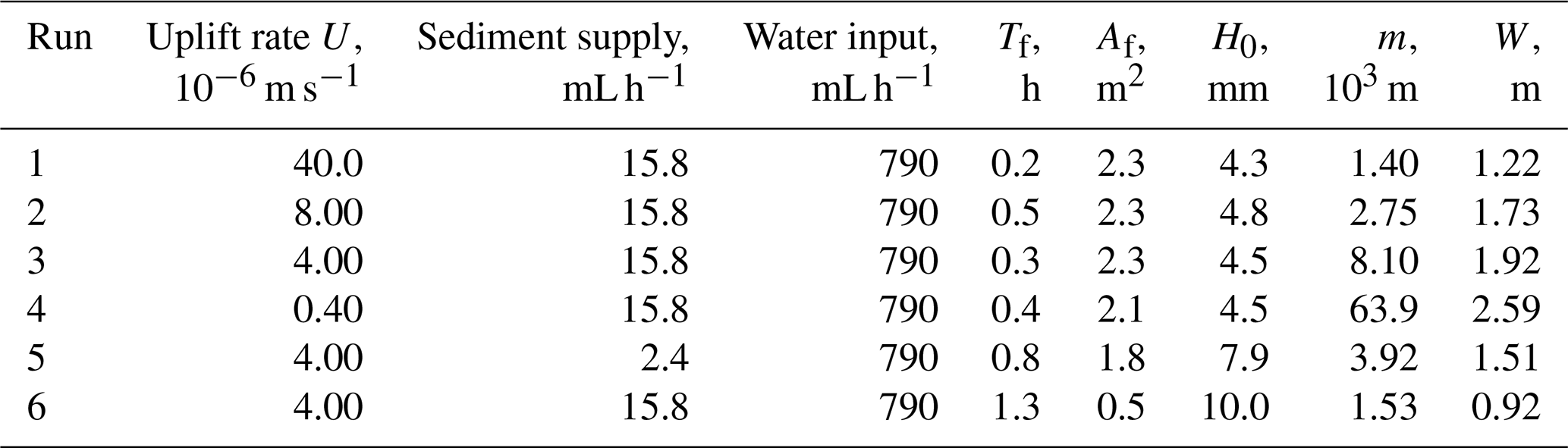
Testing the model provided in Eq. (15) requires the quantification of valley width, W, and the ratio of $q_{\mathrm{L}}/U$ or its proxy m from the experimental data. Mean valley width was calculated from the bevelled area of the fold divided by the length of the uplifted area of 0.5 m (Table 1). As U was set as a boundary condition for each run, only the lateral transport capacity, q_L, needs to be estimated from other measured experimental parameters. Because many channel parameters, such as channel width and depth, are ill-defined in the quickly evolving braided river system of the experiment, we need to define effective parameters such as representative means for a comparison with Eq. (15). Bufe et al. (2016a) measured the area that was actively reworked by channels prior to uplift, A_f [L²], and they determined a timescale over which this active area was reworked, T_f [T]. As such, A_f is equivalent to the area covered by the channel belt (Fig. 1b). Bufe et al. (2019) measured the bank height prior to uplift, H₀, on the scale of the experiment. The volume of sediment that is reworked laterally then scales with the ratio of the actively reworked area times the channel-bank height in the part of the experiment without uplift and the channel mobility timescale ($A_{\mathrm{f}}{H}_{\mathrm{0}}/T_{\mathrm{f}}$). When normalized by the length of the channel system for which these parameters are constrained, L = 0.88 m, we obtain a proxy for the amount of sediment that the channel can move laterally per unit channel length per unit time, q_L. Finally, we need to divide by uplift rate U to obtain m as

$$\begin{array}{}\text{(18)}& {\displaystyle \frac{q_{\mathrm{L}}}{U}}\propto m={\displaystyle \frac{A_{\mathrm{f}}{H}_{\mathrm{0}}}{L{T}_{\mathrm{f}}U}}.\end{array}$$

In all experiments, the average valley width across the fold was estimated as the total eroded area (red shaded area in Fig. 3a) divided by the length of the fold in the downstream direction (see Bufe et al., 2016a for details), which is equivalent to summing the width across all individual valleys.

3.2 Test 2: channels crossing folds in the Tian Shan foreland

To complement the experimental dataset, we extracted widths of valleys crossing single uplifting folds in the desert foreland of the Tian Shan, NW China (Fig. 3b–c). The Tian Shan is a major intracontinental mountain range that features uplift rates of ∼ 20–25 mm yr⁻¹ and accommodates an equivalent of 40 %–60 % of the total convergence between the Indian and Eurasian plates (Abdakhmatov et al., 1996; Zubovich et al., 2010, 2016). Along the southern and northern foreland, a series of detachment, fault-bend, and fault-propagation folds have uplifted the Cenozoic clastic basin fill of the Tarim and Junggar basins and are incised by antecedent streams that drain the Tian Shan (Avouac et al., 1993; Bufe et al., 2017a, b; Chen et al., 2007; Heermance et al., 2007, 2008; Hubert-Ferrari et al., 2007; Li et al., 2012, 2013, 2015; Scharer et al., 2004; Tapponier and Molnar, 1979; Thompson Jobe et al., 2017) Along both the southern and northern Tian Shan, we selected 12 channels crossing active folds for which kiloyear uplift rates have been estimated by a combination of optically stimulated luminescence dating and cosmogenic nuclide dating of deformed terraces (Table 2) (Bufe et al., 2017b; Gong et al., 2014; Li et al., 2015; Lu et al., 2017; Malatesta et al., 2018; Thompson, 2013). Rivers in the Kashi area (Fig. 3b), including the Kezile River on the eastern Quilitage and the Kuitun River crossing the Dushanzi anticline (Table 1), incise weakly consolidated late Miocene to Pleistocene sand, silt, and mudstones (Chen et al., 2007; Heermance et al., 2007, 2008; Scharer et al., 2004). In turn, the other valleys include deeper, older, and more indurated clastic sediments that include conglomerates. Precipitation rates are poorly constrained in the Tian Shan, but folds in the Kuche and Urumqi areas are crossed by streams that generally receive more precipitation than streams north of Kashi (Fan et al., 2020). Across all structures, we mapped the valley floor and centrelines by hand on Google Earth imagery and obtained an estimate of a characteristic valley width from the ratio of valley floor area to the length of the valley centreline. In the case of the Boguzihe River crossing the central Atushi fold, the widths of the valleys across both tributaries that cross the fold were summed. This measurement is equivalent to the method of estimating valley width from the experimental data (Bufe et al., 2016a).

Table 2 Data for the Tian Shan channels used for Test 2.

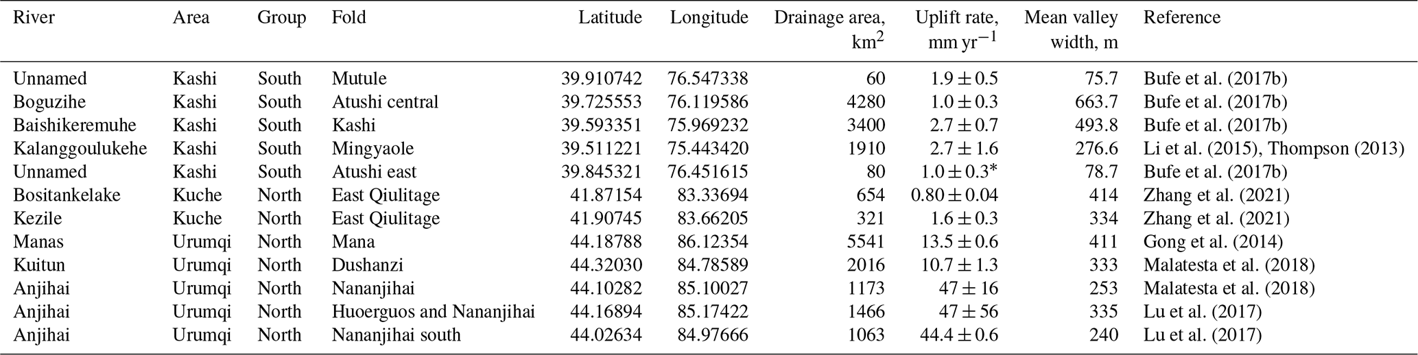
^* In the absence of kiloyear uplift rates, these rates are assumed to be equal to those of Atushi central.

To compare these measurements with the model equation, we assumed that the lateral transport capacity per unit channel length scales with drainage area, A [L²]. This assumption is consistent with experimental observations of a nearly linear scaling of lateral transport capacity and water discharge (Bufe et al., 2019; Wickert et al., 2013). As such, the proxy parameter can be calculated as

$$\begin{array}{}\text{(19)}& {\displaystyle \frac{q_{\mathrm{L}}}{U}}\sim m={\displaystyle \frac{A}{U}}.\end{array}$$

3.3 Test 3: valley width dataset from the Himalaya

Clubb et al. (2023a, b) measured valley width at more than 1.6 million locations in the Himalaya (Fig. 3d) using the method of Clubb et al. (2022), together with some auxiliary data that can be derived from topography. These include drainage area A, channel bed slope S, and the normalized steepness index k_sn, which is a measure of the slope of the channel normalized by the drainage area (e.g. Kirby and Whipple, 2001; Wobus et al., 2006). Clubb et al. (2023a, b) used SRTM data with a pixel size of 30 m and can therefore only measure valley width with a minimum width of approximately two pixels or 60 m.

Similar to the Tian Shan data (Sect. 3.2), we assume that q_L scales with drainage area. Uplift rates are not available. However, it has been shown that the normalized steepness index broadly scales with measured erosion rates in the Himalaya and in other mountain ranges (e.g. Kirby and Whipple, 2012; Lague, 2014; Wobus et al., 2006). In turn, erosion rates are a first-order proxy for uplift in the Himalaya (e.g. Hodges et al., 2004; Lenard et al., 2020; Scherler et al., 2014). Here, we assume that the relationship between uplift rate and normalized steepness index k_sn [L^0.9] is linear. Even though relationships between k_sn and erosion rate are commonly fit with nonlinear power laws, the scatter in most datasets makes a linear fit equally appropriate, both in general (e.g. Kirby and Whipple, 2012; Lague, 2014) and for the Himalaya specifically (e.g. Lague, 2014; Scherler et al., 2014). We note that A and k_sn do not correlate in the dataset (Kendall tau rank correlation coefficient = −0.036) so that the parameters can be assumed to be independent. Due to the large number of data points, we binned the data into 150 logarithmically distributed bins according to the ratio of A and k_sn. Before binning, we removed all data points with a steepness index smaller than 1 m^0.9. This threshold steepness corresponds to a channel slope of 0.2 % at a drainage area of 1 km², which we consider unrealistic for an active mountain belt. We calculated the mean and standard error of valley width and the ratio of A to k_sn for each bin. Our proxy parameter is therefore given by

$$\begin{array}{}\text{(20)}& {\displaystyle \frac{q_{\mathrm{L}}}{U}}\sim m=\stackrel{\mathrm{‾}}{\left({\displaystyle \frac{A}{k_{\mathrm{sn}}}}\right)}.\end{array}$$

Here, the overbar denotes the mean.

4 Results

4.1 Model predictions

The model predicts that valley width evolves logarithmically between two limits (Eq. 16, Fig. 4). At large values of the mobility–uplift parameter M_U, corresponding to large values of the lateral transport capacity q_L or small values of uplift rate U, the model predicts an asymptotic approach to the unconfined channel-belt width W₀ for zero hillslope sediment supply q_H (Eq. 16). Conversely, when uplift rate is high or lateral transport capacity is low (small values of M_U), the equation levels off at the channel width W_C. For intermediate M_U, valley width increases logarithmically as the lateral transport capacity increases or uplift decreases. For finite hillslope sediment supply q_H, the unconfined valley width reached at large M_U is correspondingly reduced (Fig. 4, dotted line). As M_U increases, the effect of a lateral sediment supply in narrowing the valley increases. However, the relative reduction of the excess width (W−W_C) by a lateral sediment supply relative to a case with q_H = 0 is constant, independent of M_U.

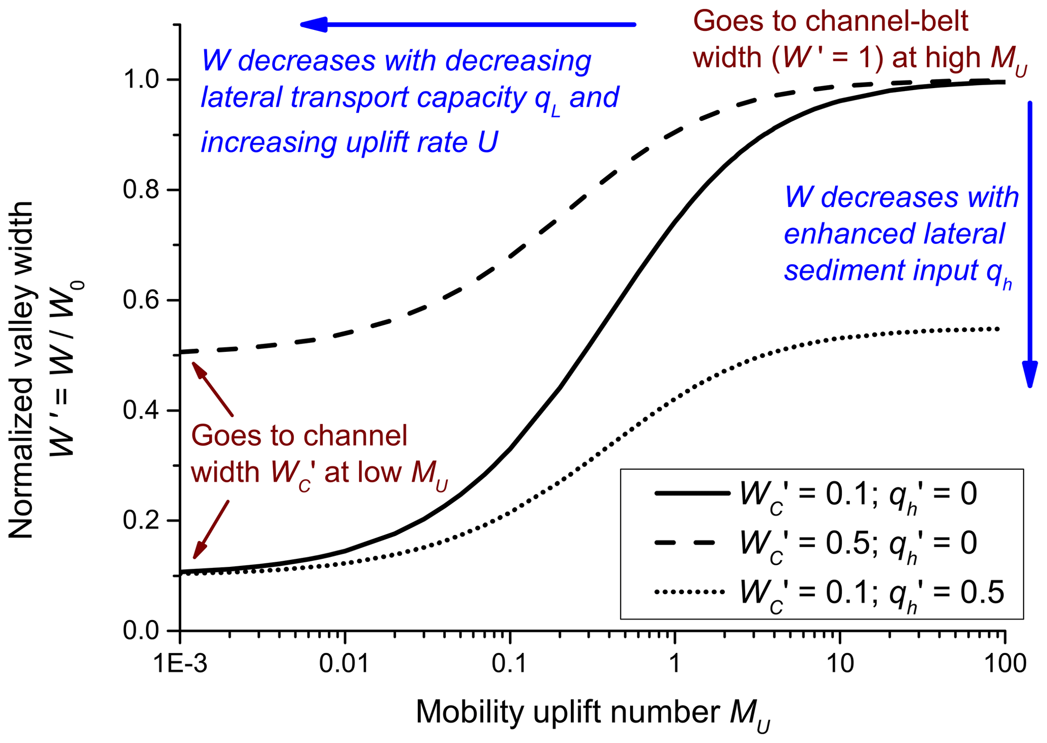
Figure 4 Evolution of dimensionless valley width as a function of the mobility–uplift number M_U, predicted by Eq. (16). An increase in M_U corresponds either to an increase in lateral transport capacity, q_L, or a decrease in uplift rate U. A change in the relative channel width $W_{\mathrm{c}}^{\prime }$ affects the left-hand limit (solid and dashed lines), while a change in the relative hillslope supply $q_{\mathrm{h}}^{\prime }$ affects the right-hand limit (solid and dotted lines).

4.2 Comparison to data

Our valley width model can closely trace the relationship between valley width and m in the experimental, Tian Shan, and Himalaya datasets (Fig. 5, Table 3). For the experimental dataset we obtained a mean unconfined valley width ${\stackrel{\mathrm{‾}}{W}}_{\mathrm{0}}=$ 2.7 m and a channel width ${\stackrel{\mathrm{‾}}{W}}_{\mathrm{C}}=$ 0.29 m, with an R² of 0.90 (Fig. 5a). The value of ${\stackrel{\mathrm{‾}}{W}}_{\mathrm{0}}=$ 2.7 m corresponds to the total width of the basin available for bevelling (Fig. 3 in Bufe et al., 2016a) and is about 22 % higher than the inferred actively bevelled width (median $A_{\mathrm{f}}/L$ = 2.22 m). The channel width varies in the experiments and often there are multiple channels. The fitted value is thus an effective value. It is around half of the minimal observed channel width of 0.50–0.56 m when flow is concentrated into a single channel.

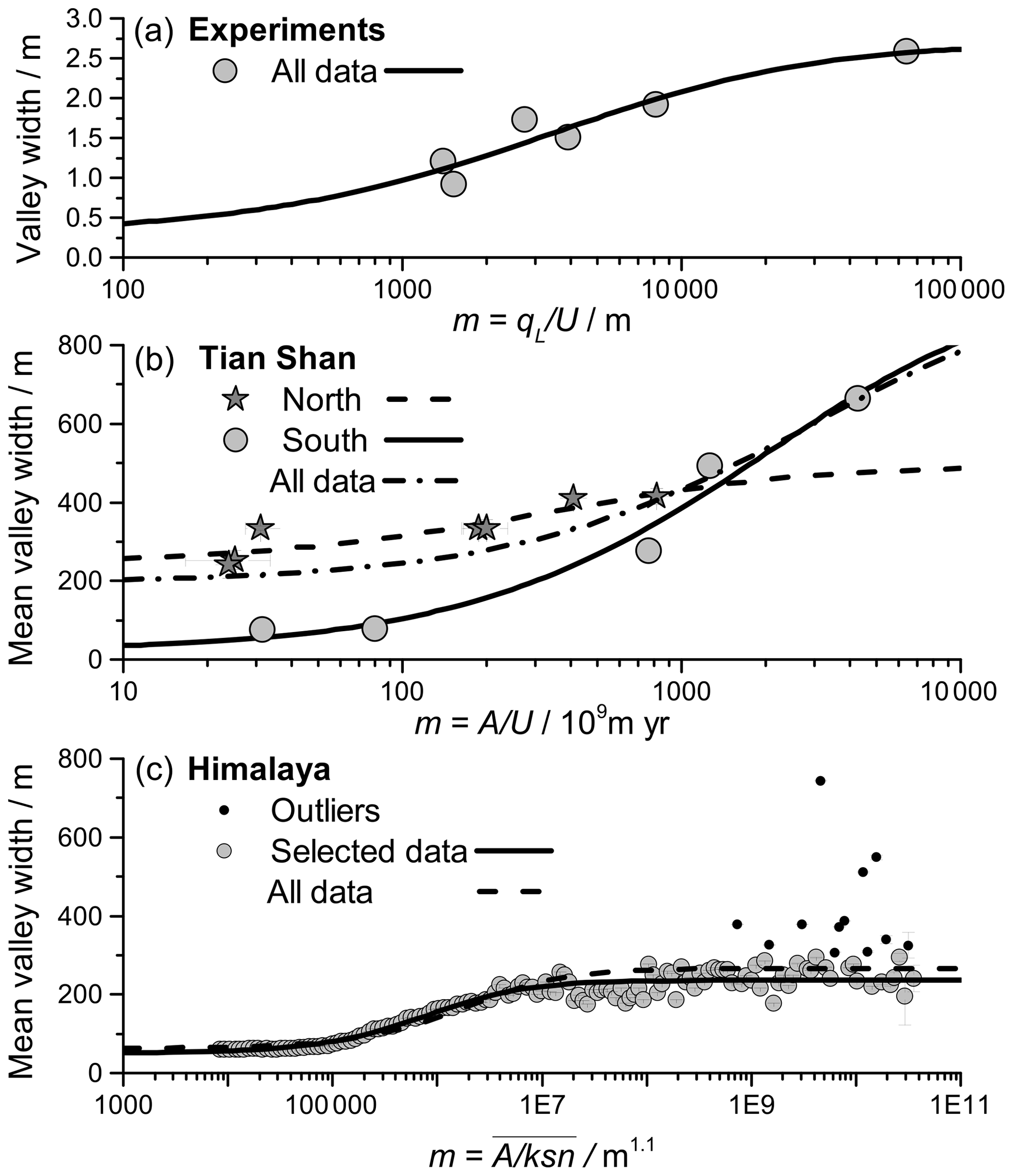
Figure 5 Valley width as a function of the proxy m for the ratio of lateral transport capacity and uplift. Lines give fits according to Eq. (17); all fit parameters are listed in Table 3. (a) Data from the analogue experiments by Bufe et al. (2016a). Mean valley width is calculated from the bevelled area of the fold divided by the length of the uplifted area of 0.5 m (Table 1). The proxy for the ratio of lateral transport capacity q_L and uplift rate U is given in Eq. (18). (b) Valley width in the Tian Shan (Table 2) as a function of the ratio of drainage area, used as a proxy for q_L, and uplift rate (Eq. 19). Values for the north (dark stars, dashed line) and south (grey dots, solid line) are treated separately. The dash-dotted line shows a fit to all data. (c) Mean valley width shown as a function of the mean ratio of drainage area A and the steepness index k_sn, with the latter assumed to linearly scale with uplift rate (Eq. 20). Error bars show the standard error of the mean for all values within a bin. We assumed that values of k_sn < 1 are unrealistic. If all remaining data points are included, the fit yields R²= 0.63 (dashed line). However, assuming that valleys with a mean width above 300 m are dominantly formed by processes other than fluvial bevelling, some of the data points can be treated as outliers (black circles). The remaining data points yield R² = 0.91 (grey circles, solid line). Note that the inferred channel widths ${\stackrel{\mathrm{‾}}{W}}_{\mathrm{C}}$ are likely affected by the 30 m resolution of the digital elevation model that underlies the dataset.

Table 3 Fit values for the data tests.

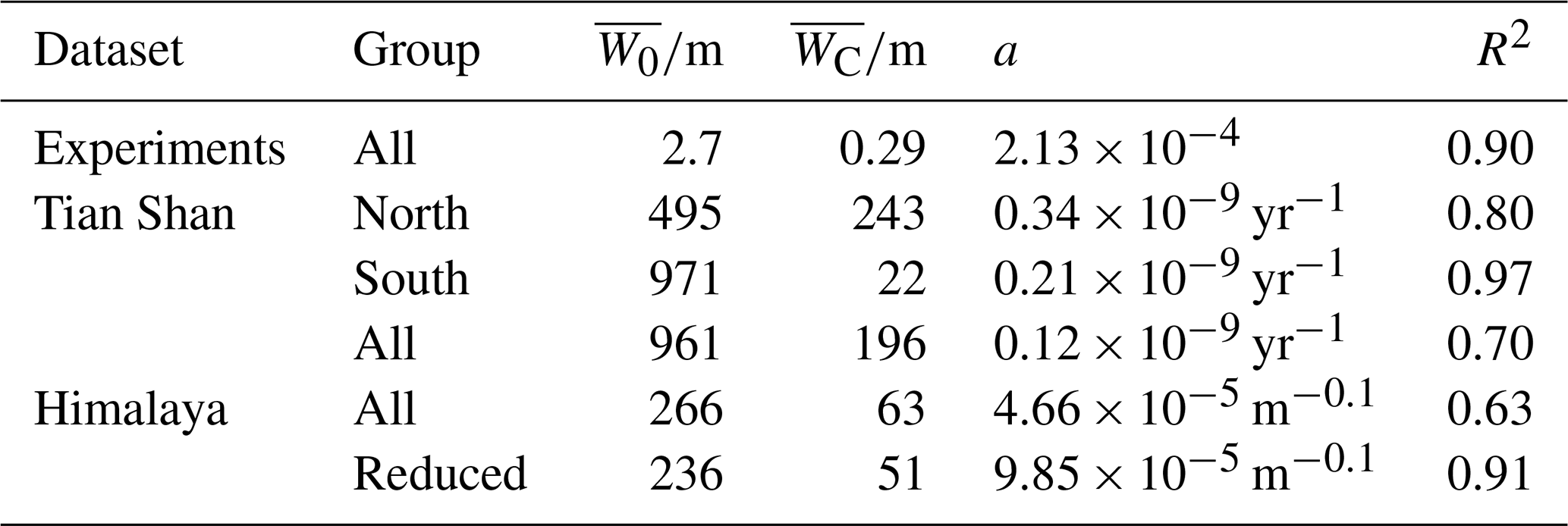
For the Tian Shan dataset, we fitted data from the north and south separately. For the north, we obtained an unconfined valley width ${\stackrel{\mathrm{‾}}{W}}_{\mathrm{0}}$ = 495 m and a channel width ${\stackrel{\mathrm{‾}}{W}}_{\mathrm{C}}=$ 243 m, with an R² of 0.80 (Fig. 5b). For the south, we obtained an unconfined valley width ${\stackrel{\mathrm{‾}}{W}}_{\mathrm{0}}$ = 971 m and a channel width ${\stackrel{\mathrm{‾}}{W}}_{\mathrm{C}}=$ 22 m, with an R² of 0.97 (Fig. 5b). Note that fitted unconfined valley and channel widths represent averages for streams with very different drainage areas (see Table 2).

The data from the Himalaya (Clubb et al., 2023b) show considerable scatter, and we performed two fits to binned means of the data points rather than to all of the data (Fig. 5c). The first fit includes all data and yielded an unconfined valley width ${\stackrel{\mathrm{‾}}{W}}_{\mathrm{0}}$ = 266 m and a channel width ${\stackrel{\mathrm{‾}}{W}}_{\mathrm{C}}=$ 63 m, with an R² of 0.63. For the second fit, we excluded all bins with a mean valley width above 300 m. These high valley widths appear as outliers at in the data (Fig. 5c), and we suggest that the widest valleys were dominantly formed or modified by processes other than the fluvial bevelling assumed in the model, for example glacial erosion, alluvial valley infilling, or large-scale landsliding (e.g. Harbor, 1992; Montgomery, 2002; Stolle et al., 2017; Zakrzewska, 1971). For this fit, we obtained an unconfined valley width ${\stackrel{\mathrm{‾}}{W}}_{\mathrm{0}}=$ 236 m and a channel width ${\stackrel{\mathrm{‾}}{W}}_{\mathrm{C}}=$ 51 m, with an R² of 0.91 (Fig. 5c). The estimate of channel width is likely affected by the 30 m resolution of the digital elevation model that underlies the dataset, which hampers the identification of valleys that are narrower than about 60 m.

4.3 Downstream variation of valley width

Our model was derived by considering valley formation in a cross-section. However, the model can also yield predictions on how valley width develops with changing drainage area along a channel because channel width, W_C, unconfined channel-belt width, W₀, and lateral transport capacity, q_L, all depend on water discharge. We can compare the predictions for the scaling between valley width and drainage area from our model with existing data. Based on empirical observations, multiple authors (e.g. Beeson et al., 2018; Brocard and van der Beek, 2006; Clubb et al., 2022; Langston and Temme, 2019; May et al., 2013; Snyder et al., 2003; Tomkin et al., 2003) have suggested that valley width scales with drainage area according to a power law of the form

$$\begin{array}{}\text{(21)}& W=k_{\mathrm{W}}{A}^{\mathit{\omega }}.\end{array}$$

Here, we compiled information on the scaling exponent from various studies (Table 4) and compare them to predictions from our model.

Table 4 Scaling of valley width and drainage area.

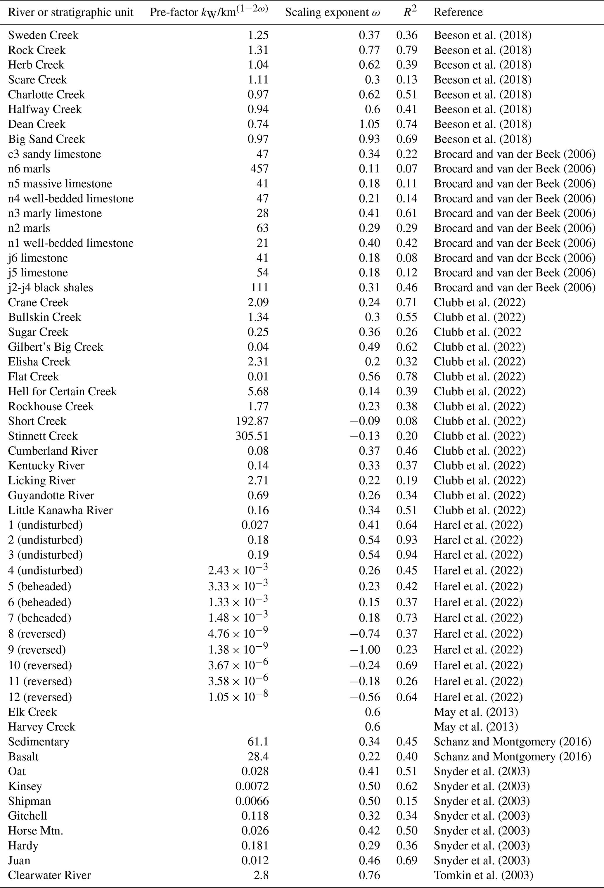
In the limits of the model for small and large M_U, we expect the valley width to approach the channel width W_C or the unconfined valley width W₀, respectively. Therefore, at these limits, the scaling between valley width and drainage area should follow the scaling between drainage area and W_C and between drainage area and W₀, respectively. Because the latter parameter scales with flow depth (Eq. 8), we need to consider the drainage area scaling for channel width and flow depth. Channel width W_C and flow depth h also commonly scale with drainage area (e.g. Ferguson, 1986; Gleason, 2015; Leopold and Maddock, 1953; Park, 1977; Rhodes, 1978). The W_C−A scaling exponent typically varies between about 0.3 and 0.6, with a most commonly cited value of 0.5 (e.g. Ferguson, 1986; Gleason, 2015; Leopold and Maddock, 1953). In turn, the h−A scaling exponent typically varies between 0.2 and 0.5, with a most commonly cited value of 0.4 (e.g. Ferguson, 1986; Gleason, 2015; Leopold and Maddock, 1953). However, for both exponents, values that are higher or lower than the stated range are not uncommon. For example, Park (1977) gives a range between 0.09 and 0.70 for the h−A scaling exponent and between 0.03 and 0.89 for the W_C−A scaling exponent from a global data compilation. Rhodes (1978) gives a similar range between 0.01 and 0.84 for the h−A scaling exponent and between 0 and 0.84 for the W_C−A scaling exponent. As a result, based on Eqs. (8) and (15), our model predicts that valley width W should increase with drainage area A according to a power law with an exponent between 0.03 and 0.9 and the most likely value of 0.4–0.5 (Park, 1977; Rhodes, 1978). The range of the W−A scaling exponent ω compiled from the literature (Table 4) corresponds well to these expected ranges (Fig. 6).

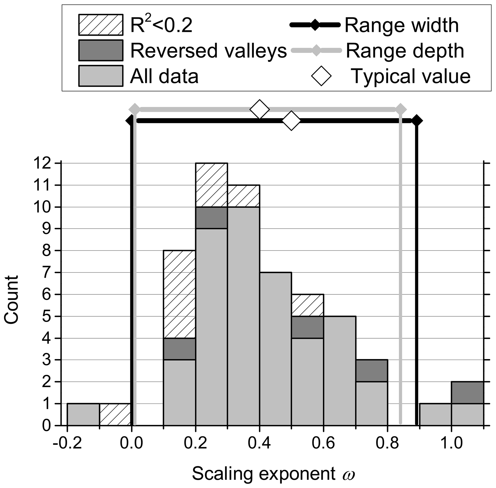
Figure 6 Histogram of 57 valley width to drainage area scaling exponent ω (Eq. 21), compiled from the literature (Table 4). Light grey blocks give all data from regular valleys with a correlation coefficient R² between valley width and drainage area exceeding 0.2, striped blocks give data with R² < 0.2, and dark grey blocks correspond to reversed valleys reported by Harel et al. (2022), where tilting reversed the flow direction of the river. The ranges of scaling exponent values for flow depth (grey; 0.01–0.84) and channel width (black; 0–0.89) reported by Park (1977) and Rhodes (1978) are also indicated (see Eq. 8).

The scaling factor k₀ between channel-belt width and flow depth (Eq. 8) cannot be accurately constrained with the presently available data. For the experimental dataset, Bufe et al. (2016a) estimated the flow depth at 7.5 mm, which implies k₀ = 321 (Table 3). A value of k₀ of the order a few hundred also seems to be reasonable when considering the field data (compare to Table 3).

5 Discussion

5.1 Model concept

Our model predicts the scaling of valley or channel-belt width with flow depth, bank height, and channel width (Eq. 8) and how this valley width is modulated by uplift and lateral hillslope sediment supply (Eq. 15). It is, essentially, a deterministic steady-state model for valley width, building on the stochastic concept of a river channel migrating across an alluviated floodplain and switching direction according to a Poisson process. The model reproduces the relationships between valley width and the ratio of lateral channel mobility and uplift in three separate datasets (Fig. 5). In addition, it predicts a range of scaling exponents between valley width and drainage area that is consistent with those observed in natural settings (Fig. 6). As such, it has quantitative explanatory power that expands previous efforts focusing on the transient widening phase (Martin et al., 2011; Hancock and Anderson, 2002), non-uplifting valleys (Tofelde et al., 2022), or empirical (e.g. Langston and Temme, 2019; Brocard and van der Beek, 2006; Beeson et al., 2019), numerical (Langston and Tucker, 2018), and qualitative (Clubb et al., 2023a) descriptions of valley formation. In addition, the model, in principle, encompasses all currently known controls on steady-state valley width (see Martin et al., 2011; Tofelde et al., 2022) and yields a wealth of testable predictions. For example, it yields an equation for channel-belt width (Eq. 8) and predicts that valley width is controlled by four dimensionless numbers (Eq. 15). Our model predicts that fluvial valley width is controlled by both climatic and tectonic conditions but is explicitly independent of lithology at steady state. While tectonics come into the model via the uplift rate, climate appears indirectly, either as a control on unconfined channel-belt width in the limit of low uplift rate or as a control on channel width in the high uplift rate limit. Likewise, lithology exerts an implicit, indirect control by changing channel width (see Sect. 5.3).

The good fit of our model to multiple datasets ranging from rivers crossing a single fold to an entire orogen suggests that many valleys, especially at small drainage areas and/or high uplift rates, are formed to first order by laterally migrating rivers. We note that the Himalayan data are characterized by large scatter that can arise from multiple factors, such as variations in sediment grain size and lithology, unequal distributions of rainfall, non-steady-state valleys, response to transient nonuniform uplift, or the dominance of processes other than fluvial bevelling in setting valley width. Yet, our model provides an excellent fit to the binned means of the data (R² = 0.91), especially when bins with mean valley width exceeding about 300 m are excluded (Fig. 5c). Hence, we suggest that the model can be applied to a wide variety of physiographic settings. The two field datasets that we used for our tests originate from active mountain belts, the Tian Shan (Sect. 3.2) and the Himalaya (Sect. 3.3). As such, these channels are likely controlled by bedrock and probably cannot be considered to be fully alluvial rivers. We suggest that in bedrock rivers, valley widening occurs dominantly during times when there is no active bedrock incision and the bedrock floor of the valley is covered by sediment such that the river behaves like an alluvial river (compare Shepherd, 1972; Turowski et al., 2013). This notion is in line with recent experiments of Langston and Robertson (2023), who found that high sediment supply, sediment cover on the bed, and laterally mobile channels in the alluvium are needed for the formation of wide bedrock valleys. This means that the fill needs a depth equal to or exceeding the flow depth. As the river sweeps laterally through the sediment fill, it occasionally erodes the walls and removes the sediment that is provided from the walls by hillslope erosion (Tofelde et al., 2022) until a steady-state valley width is achieved. As such, the composition and erodibility of the valley walls should affect the speed of widening during the transient phase but not the steady-state valley width.

Many mountain rivers split into multiple channels, at least during low-flow periods. The question of whether multiple channels for the same water and sediment supply lead to different valley width cannot be fully answered at the moment, but we can make a few generic and observational statements. First, multiple channels add considerable complexity. For example, there is no requirement that all channels at all times migrate into the same direction, implying that the channels interact and that their number, size, and shape evolve over time. Incorporating this complexity into the model would require a number of additional assumptions (on channel merging, splitting, migration) and a scheme to keep track of their motion within the cross-section to map their individual contributions to valley widening. Such a scheme is beyond our first simplified attempt to address the problem but yields interesting questions for future research. Second, Bufe et al.'s (2016a) experiments, which we compared to the model (Sect. 3.1), frequently featured multiple channels. Still, the model provides a reasonable explanation of the data (Fig. 5a), potentially indicating that migration of multiple channels produces an average rate and pattern of lateral sediment reworking that scale similarly to those of a single migrating channel. Third, we do not fully understand the controls on lateral transport capacity q_L. In braided experiments that all featured multiple channels, Bufe et al. (2019) found that q_L depended, among others, on water discharge, sediment supply, and grain size. Importantly, Bufe et al.'s (2019) analysis suggests that q_L scales approximately linearly with water discharges in these braided systems. Such linear scaling implies that valley widths could be independent of the detailed distribution of water between single or multiple channels, as long as all channels contribute to lateral sediment reworking and valley wall erosion according to their individual water discharge. The crucial question for the effect of multiple channels on valley width seems to lie in the way the different channels interact by merging, splitting, crossing, and affecting each other's speed as well as the rate of changing the direction of lateral migration.

5.2 Valley width scaling with drainage area

Our model predicts that valley width is equal to channel-belt width W₀ in the limit of low uplift rates and to channel width W_C in the limit of high uplift rates (Eq. 15). These two limits are important to consider because they potentially apply to a large proportion of data in natural settings. In all datasets, as well as in the model, the logarithmic dependence of valley width on lateral transport capacity and uplift rate exists across 2–3 orders of magnitude of the $q_{\mathrm{L}}/U$ ratio (or the proxy parameter m) (Fig. 5). In natural settings, this ratio can span up to 8 orders of magnitude (Fig. 5c) so that most natural valleys sit at either the W_C or W₀ limit. Using these two limits, we will in the following discuss the scaling relationship between valley width and drainage area.

In our model, channel-belt width is proportional to the square of flow depth h divided by bank height H₀ (Eq. 8). In a situation without uplift, it seems reasonable to assume that bank height, on average, corresponds to flow depth. After all, the river cannot deposit sediment at heights above its flow surface, and if the bank is lower, the flow overtops it, widens, and becomes shallower or finds a different course. Yet, there may be some variability in the bank heights due to autogenic changes between incision and deposition phases in and along the river channel (Mizutani, 1998; Bufe et al., 2019). Such changes lead to variations in channel width and depth, which can lead to variations in bank height encountered by the river throughout the floodplain, in turn affecting the W−A area scaling exponent. Further, along-stream variations in uplift or lateral channel mobility q_L – which is affected, for example, by grain size – may affect the scaling exponent. Overall, the range of observed values of the scaling exponent (Table 3) matches the expected range from hydraulic geometry quite well (Fig. 6). High values may arise from specific local conditions, other active processes, or along-stream gradients in the control variables such as uplift rate. These would need to be investigated locally in specific case studies.

In model construction, we have not explicitly considered the response of channel geometry to uplift. It is widely accepted that incising channels are narrower and deeper than non-incising or depositing channels at the same water discharge and sediment supply (e.g. Lavé and Avouac, 2001; Turowski, 2018; Yanites et al., 2010). Channel-belt width W₀ dominantly depends on flow depth (Eq. 8), and valley width is close to channel-belt width for low uplift rates. When the mobility–uplift number M_U is large, an increase in uplift rate may thus indirectly lead to an increase in valley width because the river responds to the increase in uplift with a decrease in flow width and an increase in flow depth. We expect that this counterintuitive result is applicable only in rare circumstances, when a change in uplift rate is large enough to cause an observable change in valley width due to the change in flow depth, but not so large that the direct control of uplift rate on valley width dominates.

5.3 Lithological controls on steady-state valley width

Multiple observations point to a lithological control on valley width and indicate that valleys carved into more erodible rock tend to be wider than valleys carved into less erodible lithologies (e.g. Bursztyn et al., 2015; Keen-Zebert et al., 2017; Moore, 1926; Schanz and Montgomery, 2016). For example, Lifton et al. (2009) found a negative correlation between local valley width and rock strength measured with the Schmidt hammer rebound value. Brocard and van der Beek (2006) and Langston and Temme (2019) observed higher scaling exponents in the relationship of valley width and drainage area in softer rocks compared to harder rocks. These observations contrast with the absence of a correlation of valley width with lithological units in the Himalaya, as reported by Clubb et al. (2023a). Our findings from the Himalaya suggest that a majority of valleys may be close to one of the valley width limits, where valley width approaches either the channel width W_C or the channel-belt width W₀ (Fig. 5c). It is likely that lithology influences the former limit because the width of bedrock channels in mountain regions increases with increasing erodibility (e.g. Turowski, 2018). Further, our model suggests that the channel width – and therefore any lithologic control on channel width – affects the shape of the model curve beyond the limit of small mobility–uplift numbers (see the solid and dashed lines in Fig. 4). From field observations, we expect that channel width varies by a factor below 10 for various lithologies (e.g. Ehlen and Wohl, 2002; Spotila et al., 2015). For example, Montgomery and Gran (2001) reported a halving of channel width of a river crossing from a limestone into a granite reach, and Spotila et al. (2015) observed a maximum factor of 5 for different lithologies for channel width after normalizing for drainage area. As such, the observed lithological dependence of valley width (e.g. Brocard and van der Beek, 2006; Langston and Temme, 2019; Schanz and Montgomery, 2016) is consistent with our model. In addition to the channel width, lithology may also influence the balance between hillslope sediment supply and removal. We posit that the scaling relationship between valley width and drainage area is implicitly dependent on lithology in our model, chiefly via the dependence of channel width on lithology. This dependence can be expected to emerge when scaling relationships in individual valleys or local controls are studied (as done, for example, by Brocard and van der Beek, 2006; Langston and Temme, 2019 and Lifton et al., 2009) but should disappear when data from many different valleys are averaged within a regional perspective (as done by Clubb et al., 2023a).

5.4 Comparison to previous models

Our model concept both contrasts with and builds on previous models of fluvial valley formation (Fig. 7; compare Clubb et al., 2023a; Hancock and Anderson, 2001; Martin et al., 2011; Tofelde et al., 2022). We classify existing models using two criteria (Fig. 7). First, we distinguish transient from steady-state models. Second, we distinguish models that emphasize vertical from those that emphasize lateral processes. This latter distinction essentially corresponds to the alluvial and bedrock categories proposed by Clubb et al. (2023a), in which the alluvial model emphasizes vertical processes and the bedrock model lateral processes.

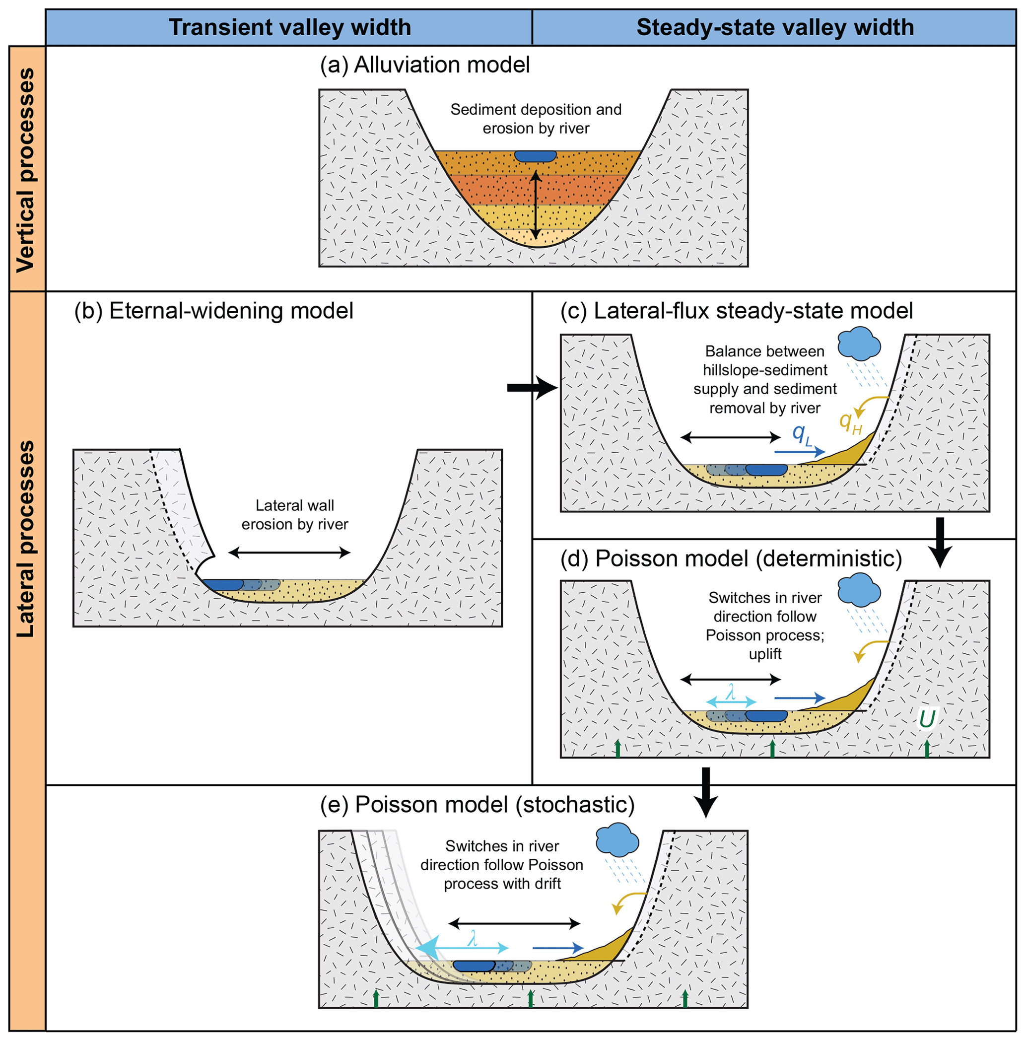
Figure 7 Overview of the existing models, organized into groups according to whether they emphasize vertical or lateral processes (vertical axis) and whether they yield a transient or steady-state valley width (horizontal axis). See text for model descriptions.

In the alluvial model (Fig. 7a), valley width is set by depositing sediment into a pre-existing V-shaped valley, created during an earlier incision phase. Because the channel bed is located on the surface of the sediment fill, valley width is set passively to the width determined by the slanting valley walls at the height of the sediment fill. Valley width is thus set by the angle of repose and the amount of sediment delivered from upstream. The alluvial model includes both transient and steady-state elements.

The eternal widening (EW) model (Fig. 7b) is a transient model emphasizing lateral processes. It assumes that the valley floor grows by fluvial undercutting of the valley walls and subsequent wall collapse (e.g. Hancock and Anderson, 2002; Malatesta et al., 2017; Martin et al., 2011; Langston and Tucker, 2018). It exists in several variants that differ in the precise formulation of the erosion model and the description of channel dynamics. In the EW model, valley width is a function of the widening or wall erosion rate integrated across the duration of widening (Hancock and Anderson, 2002; Suzuki, 1982). Although the widening rate decreases as valleys grow wider through time – because the fraction of time the river spends cutting into the walls declines (Hancock and Anderson, 2002) – the valley never reaches a steady-state width. Valley width thus depends on the widening rate and the time since the last incision event. Tofelde et al. (2022) added the notion of channel-independent hillslope sediment delivery to the EW model (Fig. 7c). In the case of this lateral flux steady-state model, valleys can achieve a steady-state width when sediment supply from hillslopes and evacuation by the river are balanced (Eq. 12).

Within the present contribution, we add the concept that rivers randomly change the direction of migration, according to a Poisson process (Fig. 7d). This yields an average switching timescale for channel migration, setting an average bevelled width. Assuming that steady-state width corresponds to the mean behaviour of the stochastic model, channel belts reach a steady-state width even without confinement. This steady-state channel-belt width gives a maximum width for fluvial valleys, which can be reduced due to uplift or lateral hillslope sediment input (Fig. 4). This model can be termed a deterministic version of the Poisson model.

A fully stochastic Poisson model has not been treated within the present contribution but is implicit in the assumptions underlying the derivation (Fig. 7e). Due to the random motion during the Poisson process, the channel can venture beyond the steady-state width predicted by the deterministic Poisson model. Essentially, once the steady-state width has been reached, the channel may push beyond the valley boundaries on either side of the valley. This increases the width on one side but leads to less frequent visits of the floodplain on the other side. Thereby, these parts of the valley are abandoned. We expect that this effect results in a slow lateral drift of the areas frequently revisited by the river after the steady-state channel belt has been established. In an uplifting area, the valley floor would thus shift laterally over time, without changing its width. Valleys in an area without uplift will widen indefinitely at an ever-slowing pace. This prediction is analogous to the eternal widening model and yields a similar outcome with a different mechanism.

Finally, we note that valley width could be set or modified by processes other than lateral erosion of the valley walls by the river or deposition and evacuation of sediment. These could be, for example, back-weathering of the walls (e.g. Krautblatter and Moore, 2014; Moore et al., 2009; Tofelde et al., 2022), downstream-sweep erosion of the river controlled by upstream conditions (Cook et al., 2014), large-scale landsliding (e.g. Beeson et al., 2018; Stolle et al., 2017), or glacial processes (e.g. Montgomery, 2002; Zakrzewska, 1971). These processes likely contribute to the scatter observed in the data and may explain some of the observed outliers (Fig. 5c).

It is beyond the scope of this paper to comprehensively test the models against each other and against data. Instead, we want to briefly outline the boundary conditions that are necessary for the different models to apply. Clubb et al. (2023a) found a strong inverse correlation of valley width with the channel steepness index k_sn in their data (Fig. 4c) but no correlation with lithological units. They argued that this observation rules out the dominance of lateral processes (Fig. 7b) and instead suggested that the alluvial model (Fig. 7a) prevails, where valley width is mainly set by sediment deposition and evacuation in a previously existing V-shaped valley. Clubb et al. (2023a) suggested that high uplift rates lead to elevated channel bed slopes and that the river responds by deposition to build these slopes in a pre-existing valley. However, substantial deposition of sediment following the incision of a valley can only occur (i) if there is a substantial increase in the ratio of upstream sediment supply to water discharge, (ii) if the relative base level rises, or (iii) if the stream is disconnected from the original base level, which is possible, for example, when the channel is blocked by a massive landslide (e.g. Korup, 2006). Thus, we expect that, in an uplifting landscape, filled valleys generally present transient features. Case (i) can occur if either climatic conditions change (affecting both sediment supply and discharge) or upstream uplift rates increase (affecting downstream sediment supply). A comparison of different valleys is then only meaningful if a similar change occurs in all basins at the same time. This seems unlikely given the wide range of climatic and tectonic conditions within the Himalaya. Case (ii) can occur if the relative base-level uplift rate increases. Further studies are necessary to investigate whether the spatial or temporal variations in uplift rate for catchments in the Himalaya are consistent enough to cause major base-level changes and sediment aggradation of V-shaped valleys that are correlated across the range. Further, a comparison of different catchments would only be meaningful if the change in uplift occurs at the same time. In case (iii), the river disconnects from the downstream base level, and as a result, the channel is insensitive to the uplift. Assuming the upstream regions keep eroding at the same rate as prior to the disconnection, the amount of deposited sediment – and therefore valley width – should scale positively with uplift rather than negatively, contradicting the observation from the data from the Himalaya.

In contrast, our model implies that the role of uplift is to increase the thickness of alluvium that the river has to move through when migrating laterally – thereby slowing the lateral back-and-forth movement of the river and narrowing the valley. This uplift effect does not consider changes in sediment supply that could be driven by increased landscape-scale erosion rates. Such an effect can be modelled in the form of modulating lateral transport capacity q_L. As argued in Sect. 5.3, our model is consistent both with an absence of lithological control on the regionally averaged steady-state valley width (Clubb et al., 2023a) and with emerging lithological controls in the scaling relationships of individual valleys (Brocard and van der Beek, 2006; Langston and Tucker, 2019). As explained above, we propose that the erosion rate of valley walls by the river modulates the transient rate of widening up to the steady state. In turn, at steady state the river does not actively erode valley walls, but the steady-state valley width is limited either by the rate of lateral sediment input from hillslope erosion processes (Tofelde et al., 2022) or the likelihood of channel switching within the valley. Of course, in an uplifting setting, the river has to incise bedrock. In our concept, incisional and widening phases of the river are separated, as has been suggested previously (e.g. Martin et al., 2011; Hancock and Anderson, 2001), but it is not necessary that the incisional phases at all times carve deep V-shaped valleys that are subsequently filled up. Many mountain rivers feature a closed sediment cover during low and intermediate flows (e.g. Tinkler and Wohl, 1998; Turowski et al., 2013), with a thickness of a few metres – enough for a river to sweep back and forth across the valley within the alluvium. In turn, vertical incision dominantly occurs during large floods (e.g. Cook et al., 2018; Lamb and Fonstad, 2010). Turowski et al. (2013) suggested that rivers alternate between the deposition and evacuation of sediment during floods and intermediate flow because transport capacity and sediment supply both depend on, but scale differently with, discharge. Whether a particular river is “flood-cleaning”, i.e. it evacuates sediment during big events, or “flood-depositing”, i.e. it deposits sediment during big events, depends on site-specific conditions relating to hydrology, substrate, climate, and channel morphology.

In cases where valleys are deeply infilled (Blöthe et al., 2014; Wang et al., 2014), the river moves laterally through the fill and widens the valley when encountering the bedrock walls. If the valley width imposed by the fill – as in the alluvial model (Fig. 7a) – exceeds the steady-state width, infilled valleys may be wider than predicted by Eq. (15). This can potentially explain some of the observed outliers (Fig. 5c).

6 Conclusions

Within this contribution, we have derived a physics-based steady-state model for the width of channel belts and river valleys. In agreement with previous suggestions, we assume that valleys widen by river undercutting of valley walls. We add the notion of random changes in the river's direction of motion, which can be described by a Poisson process. We link the probability of switches per unit time to the river's lateral mobility (Bufe et al., 2019), as well as channel depth and width. We derive a deterministic steady-state model for fluvial valley width that can account for currently known controls, including channel lateral mobility (Bufe et al., 2019), discharge and sediment supply (e.g. Beeson et al., 2018; Tomkin et al., 2003), lateral hillslope sediment supply (Tofelde et al., 2022), uplift or incision rate (Bufe et al., 2016a; Clubb et al., 2023a), the absence of a correlation with lithology in a regional perspective (Clubb et al., 2023a), and lithological controls on scaling relationships of individual valleys (Brocard and van der Beek, 2006; Langston and Tucker, 2019). The model predicts that for low uplift rates, valley width is equal to channel-belt width, and for high uplift rates, it is equal to channel width. A logarithmic function connects these two limits for intermediate uplift rates (Fig. 4, Eq. 15). The model corresponds well to field and experimental data on valleys in uplifting settings (Fig. 5).

The model yields a wealth of quantitative predictions that can, in principle, be tested against experimental and field data. Its analytical equation can be used to track valley width in models of river corridors (e.g. Gasparini et al., 2007; Heimann et al., 2015; Wickert and Schildgen, 2019) or entire landscapes (e.g. Barnhart et al., 2020; Gailleton et al., 2024). It thus may allow for more comprehensive descriptions of mountain landscapes or the interaction of rivers with their floodplains.

Appendix A

Symbols	Notation
λ	Rate parameter of Poisson processes describing the switch in the direction of river motion [T−1]
a	Scaling parameter (varying units)
A	Drainage area [L2]
Af	Area actively reworked by channel prior to uplift in experiments [L2]
c	Dimensionless constant of order 1 [−]
h	Flow depth [L]
H+	Height of the riverbank in the direction of river motion [L]
H−	Height of the riverbank opposite the direction of river motion [L]
H0	Constant bank height in conditions without tectonic uplift [L]
k	Dimensionless constant [−]
k0	Dimensionless constant, defined by $c/k$ [−]
ksn	Normalized steepness index [m0.9]
kW	Pre-factor in the power-law scaling between valley width and drainage area [L1−ω]
m	Proxy that scales with $q_{\mathrm{L}}/U$ (varying units)
MU	Mobility–uplift number, MU = $q_{\mathrm{L}}/U{W}_{\mathrm{0}}$ [−]
qH	Rate of lateral sediment supply from hillslopes or valley walls per channel length [L2 T−1]
$q_{\mathrm{H}}^{\prime }$	Normalized hillslope sediment supply, $q_{\mathrm{H}}^{\prime }=q_{\mathrm{H}}/q_L$[−]
qL	Lateral transport capacity, i.e. the amount of sediment that the channel can move by lateral erosion per
	unit channel length per unit time [L2 T−1]
P	Fraction of time that a river spends at any of its channel walls or valley margins [−]
Δt	The characteristic length of time the river moves on average in the same direction [T]
Tf	Timescale over which Af was reworked [T]
U	Uplift rate [L T−1]
v	Lateral speed of the river as it reaches valley floor margins, i.e. wall toes [L T−1]
V	Lateral migration speed, i.e. the speed of river migrating back and forth across the valley floor [L T−1]
W	Valley floor width [L]
W′	Normalized valley width, $W^{\prime }=W/W_{\mathrm{0}}$[−]
WC	Width of the river channel [L]
$W_{\mathrm{C}}^{\prime }$	Normalized channel width, $W_{\mathrm{C}}^{\prime }=W_{\mathrm{C}}/W_{\mathrm{0}}$ [−]
$\stackrel{\mathrm{‾}}{W_{\mathrm{C}}}$	Average channel width [L]
W0	Channel-belt width or unconfined valley width [L]
$\stackrel{\mathrm{‾}}{W_{\mathrm{0}}}$	Average channel-belt width [L]
ω	Scaling exponent in the power-law scaling between valley width and drainage area [−]