A fractal framework for channel–hillslope coupling

Questions of landscape scale in coupled channel–hillslope landscape evolution have been a significant focus of geomorphological research for decades. Studies to date have suggested a characteristic landscape length that marks the shift from fluvial channels to hillslopes, limiting fluvial incision and setting the length of hillslopes. The representation of real-world landscapes in slope–area plots, however, makes it challenging to identify the exact transition from hillslopes to channels, owing to the existence of an intermediary colluvial valley region. Without a rigorous explanation for the scaling of the channel hillslope transition, the use of computational models, which are forced to implement a finite grid resolution, is limited by the scaling of the physical parameters of the model relative to the grid resolution. Grid resolution is also tied to the width of channels, which is undetermined without a rigorous explanation of where channels begin.

Building on existing work, we demonstrate the existence and implications of the characteristic landscape length and its relationship to grid resolution. We derive the characteristic landscape length as the horizontal length in a one-dimensional landscape evolution framework required to form an inflection point. On a two-dimensional domain, channel heads form in steady state at the characteristic area, the square of the characteristic length, independent of grid resolution. We present a box-counting fractal definition using the grid resolution, revealing that the dimension of the contributing drainage region on steady-state hillslopes is expressed as a multifractal system. In sum, channels have contributing drainage areas, therefore a dimension of 2, whereas, by definition, unchannelized locations or nodes have a dimension between zero and 2, so not a well-defined area. This conceptualization aligns with the scaling of channel width as the square root of drainage area. Since channel heads form at a resolution-independent drainage area, the width of channel heads is not explicitly defined, suggesting that the grid resolution is analogous to the property of channel head width in real-world landscapes, influenced by the particle size. We substantiate this theory with topographic analyses of Gabilan Mesa, California. These findings clarify several unresolved properties of channel–hillslope coupling, with potential for substantially improving the accuracy of coupled landscape evolution models in replicating landscape forms.

1 Introduction

Landscape evolution models (LEMs) are quantitative theories that describe the physical processes shaping geomorphic patterns. Coupled channel–hillslope LEMs combine both fluvial and hillslopes processes, each described by individual mathematical statements called geomorphic transport laws. A central, yet poorly understood, aspect of these coupled LEMs is channel initiation, setting the transition between hillslopes and channels (Tucker and Hancock, 2010; Dietrich et al., 2003). In real-world landscapes, this transition is often described in terms of stochastic perturbations and time-dependent behavior (Smith and Bretherton, 1972; Howard and Kerby, 1983; Del Vecchio et al., 2023). Given that landscape evolution occurs over long timescales, computationally evaluated LEMs are commonly used to test theories describing channel initiation (Anand et al., 2022; Tucker and Hancock, 2010).

Selecting a finite grid resolution is essential for both computationally evaluating two-dimensional coupled channel–hillslope LEMs and interpreting real-world topography from digital elevation models (DEMs). Scaling grid resolution relative to physically derived parameters or topography presents several challenges. The widely used stream-power incision model (Howard and Kerby, 1983; Howard, 1994; Whipple and Tucker, 1999) requires contributing drainage area as a proxy for discharge. When stream-power incision is combined with linear diffusion (Culling, 1960), the scaling of contributing drainage area across grid resolutions inconsistently affects hillslopes, with presumably parallel flow paths, and channels, where flow paths converge (Pelletier, 2010; Hergarten, 2020; Hergarten and Pietrek, 2023; Bernard et al., 2022). Previous efforts have addressed this issue by proposing criteria for channel initiation (Hergarten, 2020; Hergarten and Pietrek, 2023), but the scaling relationships between the physically derived model parameters and channel initiation remain unclear. Instead, computational models often implement a physically derived or arbitrarily chosen threshold for drainage area or the product of powers of drainage area and slope (A^mSⁿ), below which stream-power erosion is absent (Perron et al., 2008; Tucker and Bras, 1998; Campforts et al., 2017; Theodoratos and Kirchner, 2020). However, some studies have suggested that the value of the channelization thresholds themselves depends on grid resolution (Montgomery and Dietrich, 1992; Ariza-Villaverde et al., 2015; Tarboton et al., 1991), and some studies have questioned the necessity of using a threshold altogether (Perron et al., 2008; Theodoratos et al., 2018). Grid resolution also complicates the modeling of channels with large drainage areas where the expected channel widths exceed the pixel width (Pelletier, 2010; Hergarten, 2020).

Prior research has also explored the characteristic landscape length that distinguishes hillslopes from channels and defines the width of first-order valleys (Montgomery and Dietrich, 1992; Tarboton et al., 1988; Perron et al., 2008; Horton, 1945). This length is thought to be associated with the flow-path length from topographic maxima to inflection points with maximum steepness, differentiating convex summits and concave-up valleys (Willgoose et al., 1991a; Tarboton et al., 1991; Roering et al., 2007). Additionally, research indicates that this length scale corresponds to the square root of the contributing area at channel heads (Montgomery and Dietrich, 1992; Tarboton et al., 1988; Perron et al., 2008; Tucker and Bras, 1998). Researchers working on this problem have long noted three distinct regions – from hillslopes, intermediate colluvial valleys, and channels – in slope–area plots. In particular, they have been intrigued by the curved region associated with debris flows and shallow landslides, corresponding to unchannelized colluvial valleys with relatively constant slopes (Montgomery and Foufoula-Georgiou, 1993; Stock and Dietrich, 2006; Struble et al., 2023; McGuire et al., 2023). The connection between the intermediate region and debris flows is problematic, however, because curved slope–area plots appear in models and real-world landscapes without debris flows.

In this work we analytically derive the characteristic landscape length, defined as the contributing length to an inflection point in a one-dimensional analysis. On a two-dimensional domain, we use the characteristic landscape length and the pixel width as a measure to define a fractal box-counting definition. This reveals that unchannelized nodes, those with contributing drainage area less than the characteristic length squared, do not have a well-defined contributing drainage area, instead varying with the grid resolution according to their fractal dimension. In other words, when analyzed at sufficiently high resolution, the scaling relationship for contributing drainage regions, which are two-dimensional for channels (hence drainage area), breaks down on hillslopes, resulting in a system of contributing drainage dimension that does not exhibit self-similarity.

We demonstrate that this theory, derived from one-dimensional analyses and computational simulations, corresponds to real-world topography using Gabilan Mesa in California. In particular, we show that, on Gabilan Mesa, the drainage area of nodes with the steepest slope (the inflection point) scales with 1 factor of grid resolution. In contrast, the drainage area of channel heads, calculated as the square of the drainage area divided by the grid resolution at the inflection point, is independent of grid resolution. Using these results, we propose directions for computational models and suggest that real-world landscapes have a property analogous to a grid resolution.

2 Detachment-limited linear diffusion landscape evolution

Landscape evolution models for erosional drainage-basin evolution have a storied history. The simplest, most applicable model assumes detachment-limited stream-power (Howard, 1994; Whipple and Tucker, 1999) and linear diffusion (Culling, 1960), and it is commonly presented in the literature as

$$\begin{array}{}\text{(1)}& {\displaystyle \frac{\partial z}{\partial t}}=U-K{A}^m|\mathrm{\nabla }z{|}^n+D{\mathrm{\nabla }}^{\mathrm{2}}z.\end{array}$$

On a two-dimensional domain, topographic elevation, z, is a function of the horizontal coordinates x and y and of time t. This model is based on three fundamental parameters: K, D, and U. Erodibility, K, modulates the strength of the stream-powered erosion. Diffusivity, D, characterizes the strength of gravity-driven erosive processes. The uplift rate, U, represents the effects of base-level forcing, such as uplift or base-level fall. We assume that K, D, and U are constant in both space and time.

Stream-power incision corresponds to the term $K{A}^m|\mathrm{\nabla }z{|}^n$. A, the contributing area, a proxy for discharge in steady-state landscapes, is calculated for each (x,y) node on the two-dimensional domain using flow-routing vectors in the direction of steepest descent of z, such that A is a function of x, y, z, and t. $\left|\mathrm{\nabla }z\right|$ is the norm of the gradient of z. Stream-powered erosion is assumed to be detachment-limited, meaning that sediments, once detached, are not redeposited within the domain.

The values of the exponents m and n are the source of significant debate in the literature. The exponent $m=\frac{\mathrm{1}}{\mathrm{2}}$, applied to contributing area A in Eq. (1), is commonplace for two reasons. Firstly, assuming n=1, the scaling of channel slopes with the square root of drainage area is consistently observed in bedrock channels and large drainage basins, in a typical range of 0.4 to 0.55 (Whipple and Tucker, 1999; Leopold and Maddock, 1953). Throughout this work, we set n=1, inducing linear behavior of stream-powered erosion and in the range suggested by empirical studies (Whipple and Tucker, 1999; Lague, 2014). Secondly, the choice of $m=\frac{\mathrm{1}}{\mathrm{2}}$ and n=1 preserves the fundamental dimension of K as a rate. However, Eq. (1) is incorrect, since it is dependent on grid resolution, which we discuss in Sect. 2.2 and address with a nuanced solution in Sect. 5.1.

Linear diffusion (Culling, 1960), representative of mixing processes such as soil creep and bioturbation, assumes that the diffusive flux, q_d, is directly proportional to the gradient of z, given as ${\mathit{q}}_{\mathrm{d}}=-D\mathrm{\nabla }z$. The divergence of the diffusive flux, −D∇²z, can be positive or negative, indicating erosion in concave-down profiles and deposition in concave-up profiles. Linear diffusion accurately models soil-mantled landscapes with cohesive sediments and gradients significantly lower than the angle of repose (McKean et al., 1993). However, it fails to represent sediment fluxes accurately on hillslopes where local slopes approach a critical slope (Roering et al., 1999).

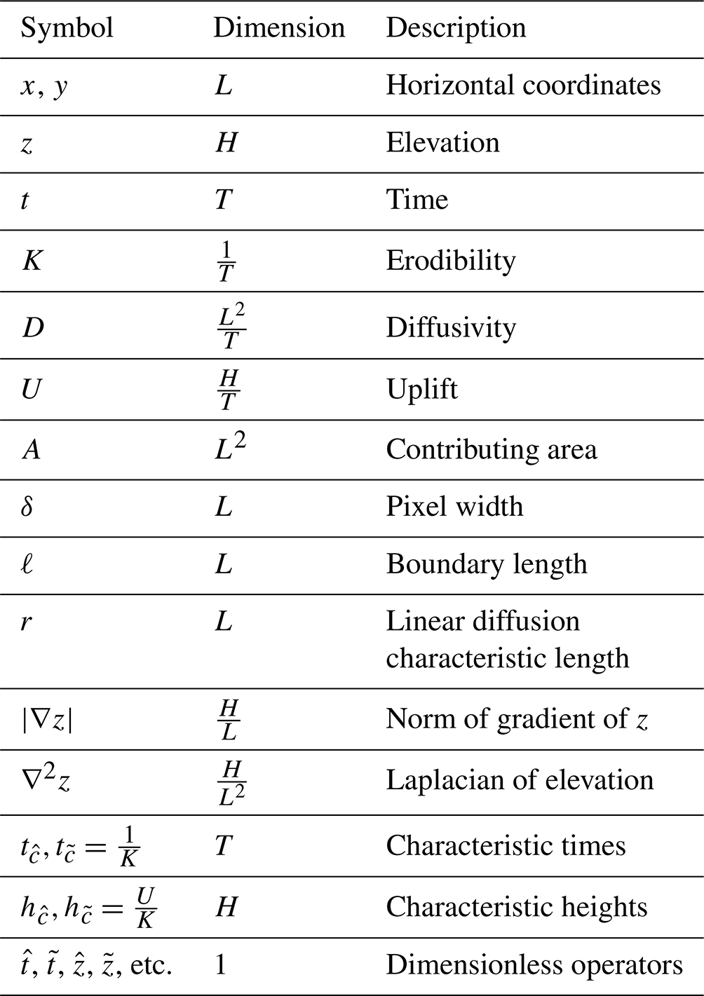
We define distinct height (H) and length (L) dimensions, in alignment with prior dimensional analyses (Theodoratos et al., 2018; Willgoose et al., 1991b). Although both H and L can be expressed in meters, treating them as separate dimensions facilitates our ability to simplify the model through non-dimensionalization (Huntley, 1967). For steady-state topography, the horizontal dimension pertains to the two-dimensional domain, while the vertical dimension serves as the function's codomain, organized so that erosion balances uplift everywhere. In Eq. (1), D has fundamental dimension L²T⁻¹ and U has fundamental dimension HT⁻¹. Throughout this work, we specify K as having the fundamental dimension T⁻¹. Table 1 summarizes the dimensions of all variables and parameters considered.

Table 1 Symbols and variable definitions used in the study.​​​​​​​

2.1 One horizontal dimension

With two horizontal dimensions, contributing drainage area scales inconsistently with grid resolution owing to differences in flow routing between hillslopes and channels. As noted by Pelletier (2010), Hergarten (2020), and Hergarten and Pietrek (2023), hillslopes are thought to have parallel flow paths, whereas channels have convergent flow paths. As these authors suggest, the area of contributing drainage regions with parallel flow paths is determined by the grid resolution, which dictates their width. In contrast, regions with convergent flow have contributing drainage areas that are relatively unaffected by changes in grid resolution. In order to address this inconsistency, we first consider the one-dimensional equivalent to the landscape evolution model presented in Eq. (1),

$$\begin{array}{}\text{(2)}& {\displaystyle \frac{\mathrm{d}z}{\mathrm{d}t}}=U-K\left|x\right|\left|{\displaystyle \frac{\mathrm{d}z}{\mathrm{d}x}}\right|+D{\displaystyle \frac{{\mathrm{d}}^{\mathrm{2}}z}{\mathrm{d}{x}^{\mathrm{2}}}},\end{array}$$

with the boundary length ℓ:

$$-{\displaystyle \frac{\mathrm{\ell }}{\mathrm{2}}}<x<{\displaystyle \frac{\mathrm{\ell }}{\mathrm{2}}}.$$

$\left|x\right|$, a length, is a proxy for the amount of the accumulated precipitation across the one-dimensional domain. The exponent m=1 preserves the fundamental dimension of K as T⁻¹ in the one-dimensional framework. Bonetti et al. (2020) present a non-dimensionalization of Eq. (2), using characteristic length $l_{\widehat{c}}=\mathrm{\ell }$, characteristic height $h_{\widehat{c}}=\frac{U}{K}$, and characteristic time $t_{\widehat{c}}=\frac{\mathrm{1}}{K}$. Therefore, $\frac{x}{l_{\widehat{c}}}=\widehat{x}$, $\frac{z}{h_{\widehat{c}}}=\widehat{z}$, and $\frac{t}{t_{\widehat{c}}}=\widehat{t}$, resulting in

$$\begin{array}{}\text{(3)}& {\displaystyle \frac{\mathrm{d}\widehat{z}}{\mathrm{d}\widehat{t}}}=\mathrm{1}-\left|\widehat{x}\right|\left|{\displaystyle \frac{\mathrm{d}\widehat{z}}{\mathrm{d}\widehat{x}}}\right|+(C_I{)}^{-\mathrm{1}}{\displaystyle \frac{{\mathrm{d}}^{\mathrm{2}}\widehat{z}}{\mathrm{d}{\widehat{x}}^{\mathrm{2}}}},\end{array}$$

$$-{\displaystyle \frac{\mathrm{1}}{\mathrm{2}}}<\widehat{x}<{\displaystyle \frac{\mathrm{1}}{\mathrm{2}}}.$$

Given the four parameters (U, D, K, and ℓ) and three fundamental dimensions (H, L, T) in Eq. (2), the equation can be rewritten using non-dimensionalization to include a single dimensionless group (Buckingham, 1914). This dimensionless group, referred to as the channelization index C_I, functions as a Péclet number and quantifies the competition between advection and diffusion in the domain (Perron et al., 2008; Anand et al., 2023; Bonetti et al., 2020).

$$\begin{array}{}\text{(4)}& C_I={\displaystyle \frac{{\mathrm{\ell }}^{\mathrm{2}}K}{D}}\end{array}$$

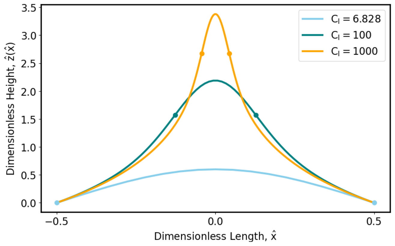
Figure 1 Equation (3) solved for various values of C_I. As noted in Anand et al. (2023), concave-down profiles are locally preserved near $\widehat{x}=\mathrm{0}$ for asymptotically large values of C_I. Inflection points are plotted with dots. The value C_I≈6.828 sets the distance between the inflection points equal to the boundary length.

Figure 1 plots the numerically evaluated steady-state profiles of Eq. (3) for various values of C_I. Larger values of C_I manifest in narrower hillslope profiles relative to the boundary size, formed by the relative strength of advective processes over diffusive processes. The computational granularity necessary for accurate numerical evaluation is a function of the channelization index, C_I. Larger values of C_I require a finer resolution to accurately represent the concave-down region around $\widehat{x}=\mathrm{0}$.

As noted by Litwin et al. (2022a), the channelization index (C_I) is a dimensionless boundary length. The intrinsic length of Eq. (2) corresponds to a group involving D, since $\left[D\right]=L^{\mathrm{2}}{T}^{-\mathrm{1}}$. To solve for this intrinsic length, we consider the fixed points of Eq. (3) (Howard, 1994). The fixed point of $\widehat{z}$, where $\frac{\mathrm{d}\widehat{z}}{\mathrm{d}\widehat{x}}=\mathrm{0}$, is located at the top of the ridge at $\widehat{x}=\mathrm{0}$. For $\widehat{x}=\mathrm{0}$, stream-powered erosion does not occur, so the steady-state dimensionless erosion at the top of the ridge is $C_I^{-\mathrm{1}}\cdot \frac{{\mathrm{d}}^{\mathrm{2}}\widehat{z}}{\mathrm{d}{\widehat{x}}^{\mathrm{2}}}=-\mathrm{1}$ (Roering et al., 2007). Inflection points, fixed points of $\frac{\mathrm{d}\widehat{z}}{\mathrm{d}\widehat{x}}$, occur at the sides of the ridge where $\left|\widehat{x}\right|\left|\frac{\mathrm{d}\widehat{z}}{\mathrm{d}\widehat{x}}\right|=\mathrm{1}$. These inflection points mark the transition from concave-down to concave-up profiles. We denote r as the length between x=0 and the inflection points of Eq. (2), identical to the characteristic hillslope length given in prior works (Roering et al., 2007; Perron et al., 2008; Willgoose et al., 1991a). For $C_I\approx \mathrm{4}+\mathrm{2}\sqrt{\mathrm{2}}\approx \mathrm{6.828}$, the inflection points of $\frac{\mathrm{d}z}{\mathrm{d}x}$ occur at $\pm \frac{\mathrm{\ell }}{\mathrm{2}}$; thus ℓ=2r. Solving for r,

$$\begin{array}{}\text{(5)}& r=\sqrt{{\displaystyle \frac{D}{K}}\left({\displaystyle \frac{\sqrt{\mathrm{2}}}{\mathrm{2}}}+\mathrm{1}\right)}\propto \sqrt{{\displaystyle \frac{D}{K}}}.\end{array}$$

For the remainder of this paper, we adopt r as the characteristic landscape length, proportional to the characteristic length-scale $\sqrt{\frac{D}{K}}$ used in several prior studies (Perron et al., 2008; Theodoratos et al., 2018). While r can also be derived from Eq. (2) as a first-order linear ordinary differential equation in $\mathrm{d}z/\mathrm{d}x$ (Appendix A), the insights gained from the non-dimensionalization of the one-dimensional equation are useful for analyzing the landscape evolution equation in two horizontal dimensions.

2.2 Two horizontal dimensions

On a two-dimensional domain, stream-power linear diffusion landscape evolution is dependent on three horizontal lengths: the landscape length r, the boundary length ℓ, and the pixel width δ. The explicit dependence on δ is controversial. On a two-dimensional domain, δ is not only correlated with numerical error, as on a one-dimensional domain, but also sets the width of linear elements, such as channels. Considering these three lengths (the boundary length, the pixel width, and r), a minimum of two dimensionless groups can be formed, without unnecessarily rescaling the other dimensional quantities (Buckingham, 1914). This approach maintains the characteristic height as $\frac{U}{K}$, diverging from the approach of Litwin et al. (2022b).

Bonetti et al. (2018) define specific area, a, a length, as the contributing area per unit contour width in the limit approaching zero contour width (Bonetti et al., 2018; Gallant and Hutchinson, 2011). Specific area, satisfying the conservation of a unitary precipitation rate, is expressed as

$$\begin{array}{}\text{(6)}& -\mathrm{\nabla }\cdot \left({\displaystyle \frac{a\mathrm{\nabla }z}{\left|\mathrm{\nabla }z\right|}}\right)=\mathrm{1}.\end{array}$$

Given δ, an infinitesimally small contour width cannot be achieved; thus a is not well defined. In the following analysis, the specific drainage area a is defined as $a=\frac{A}{\mathit{\delta }}$, while noting that the specific drainage area is implicitly dependent on the grid resolution (Litwin et al., 2022b; Costa-Cabral and Burges, 1994). Using the D8 flow-routing algorithm on a square pixel (Tarboton et al., 1988), both the flow length and the contour width between diagonal pixels measure $\sqrt{\mathrm{2}}\mathit{\delta }$ diagonally, whereas, along the cardinal directions, both metrics equal δ. With the D∞ algorithm on a square pixel, the contour width and the flow length between neighboring pixels are always δ (Gallant and Hutchinson, 2011). Throughout this paper, we use the D∞ algorithm to bypass complexities in cardinal and diagonal directions and to accurately model flow routing on divergent hillslopes.

The landscape evolution models in the form of Eq. (1) with $m=\frac{\mathrm{1}}{\mathrm{2}}$ do not explicitly address the role of flow width (Perron et al., 2008). Previous attempts to account for the channel width have sought to normalize the fluvial erosion component by a factor of $\frac{w}{\mathit{\delta }}$, where w is the channel width (Howard, 1994; Perron et al., 2008). Channel widths are observed to scale with the square root of drainage area (Leopold and Maddock, 1953); thus $\frac{w}{\mathit{\delta }}\propto \frac{\sqrt{A}}{\mathit{\delta }}$.

$$\begin{array}{}\text{(7)}& {\displaystyle \frac{\partial z}{\partial t}}& {\displaystyle }=U-{\displaystyle \frac{\sqrt{A}}{\mathit{\delta }}}K\sqrt{A}\left|\mathrm{\nabla }z\right|+D{\mathrm{\nabla }}^{\mathrm{2}}z\text{(8)}& {\displaystyle }& {\displaystyle }=U-Ka\left|\mathrm{\nabla }z\right|+D{\mathrm{\nabla }}^{\mathrm{2}}z\end{array}$$

Rescaling the stream-powered erosion by $\frac{\sqrt{A}}{\mathit{\delta }}$ defines the specific drainage area, a, a length, as the discharge source term, preserving the dimension of K. This normalization implies that fluvial erosion is proportional to contributing area, and thus discharge, assuming a uniform runoff generation rate (Litwin et al., 2022b). The calculation of a with contour width δ is appropriate for unchannelized nodes, such that erosion occurs by overland flow and that the minimum contour width is therefore δ. We first explore the implications of Eq. (8) for unchannelized nodes. The use of a ensures that the contributing drainage of locally parallel flow regions on hillslopes is independent of pixel width, thereby conforming to a one-dimensional framework. We show that locally parallel flows occur at the inflection point, a=r. For nodes without a=r, the specific drainage area is implicitly dependent on δ. This dependence is unavoidable but can be reconciled through an additional dimensionless group.

2.3 Dimensional analysis

As previously noted, considering the three horizontal lengths ℓ, δ, and r entails at least two dimensionless groups. Non-dimensionalizing Eq. (8) with $l_{\stackrel{\mathrm{̃}}{c}}=r$, $h_{\stackrel{\mathrm{̃}}{c}}=\frac{U}{K}$, and $t_{\stackrel{\mathrm{̃}}{c}}=\frac{\mathrm{1}}{K}$, such that $\frac{a}{l_{\stackrel{\mathrm{̃}}{c}}}=\stackrel{\mathrm{̃}}{a}$, $\frac{x}{l_{\stackrel{\mathrm{̃}}{c}}}=\stackrel{\mathrm{̃}}{x}$, $\frac{y}{l_{\stackrel{\mathrm{̃}}{c}}}=\stackrel{\mathrm{̃}}{y}$, $\frac{z}{h_{\stackrel{\mathrm{̃}}{c}}}=\stackrel{\mathrm{̃}}{z}$, and $\frac{t}{t_{\stackrel{\mathrm{̃}}{c}}}=\stackrel{\mathrm{̃}}{t}$, results in

$$\begin{array}{}\text{(9)}& {\displaystyle \frac{\partial \stackrel{\mathrm{̃}}{z}}{\partial \stackrel{\mathrm{̃}}{t}}}& {\displaystyle }=\mathrm{1}-{\displaystyle \frac{r}{\mathit{\delta }}}\stackrel{\mathrm{̃}}{A}\left|\stackrel{\mathrm{̃}}{\mathrm{\nabla }}\stackrel{\mathrm{̃}}{z}\right|+{\displaystyle \frac{D}{r^{\mathrm{2}}K}}{\stackrel{\mathrm{̃}}{\mathrm{\nabla }}}^{\mathrm{2}}\stackrel{\mathrm{̃}}{z}\text{(10)}& {\displaystyle }& {\displaystyle }=\mathrm{1}-\stackrel{\mathrm{̃}}{a}\left|\stackrel{\mathrm{̃}}{\mathrm{\nabla }}\stackrel{\mathrm{̃}}{z}\right|+{\left({\displaystyle \frac{\sqrt{\mathrm{2}}}{\mathrm{2}}}+\mathrm{1}\right)}^{-\mathrm{1}}{\stackrel{\mathrm{̃}}{\mathrm{\nabla }}}^{\mathrm{2}}\stackrel{\mathrm{̃}}{z}\end{array}$$

with boundary length

$${\displaystyle \frac{\mathrm{\ell }}{l_{\stackrel{\mathrm{̃}}{c}}}}={\displaystyle \frac{\mathrm{\ell }}{r}}=\mathrm{\ell }\cdot \sqrt{{\displaystyle \frac{K}{D\left(\frac{\sqrt{\mathrm{2}}}{\mathrm{2}}+\mathrm{1}\right)}}}\propto \sqrt{\left(C_I\right)}.$$

Therefore, by considering the form with the dimensionless area, this yields two dimensionless groups related to the horizontal length scales,

$${\mathrm{\Pi }}_{\mathrm{1}}={\displaystyle \frac{r}{\mathit{\delta }}},$$

with the second appearing in the boundary condition

$${\mathrm{\Pi }}_{\mathrm{2}}=\mathrm{\ell }\cdot \sqrt{{\displaystyle \frac{K}{D\left(\frac{\sqrt{\mathrm{2}}}{\mathrm{2}}+\mathrm{1}\right)}}}.$$

The dimensionless group $\frac{r}{\mathit{\delta }}$ represents the number of pixels of contributing drainage, though not necessarily individual pixels (with the D∞ flow-routing algorithm), required to form an inflection point. In the literature, some papers keep this value constant (Theodoratos et al., 2018), but others do not (Anand et al., 2023). Identical values of this dimensionless group create a consistent scaling break in steady-state slope–area space. With increased resolution, the inflection point occurs for fewer pixels of contributing area, but the same specific drainage area is calculated using contour width δ. The dimensionless ratio $\frac{\mathrm{\ell }}{r}$ denotes the boundary relative to r and is proportional to the square root of the channelization index. These dimensionless groups function similarly to two controls of a microscope: one control alters the proximity of the microscope to the specimen, effectively changing the boundary size, and the other adjusts the resolution through the focus of the lenses. The effect of these groups is demonstrated through computational simulations in the following section.

3 Two-dimensional results

We completed steady-state numerical simulations using the Landlab-equipped (Hobley et al., 2017)​​​​​​​ Jupyter notebook of Anand et al. (2023), using the D∞ algorithm (Anand et al., 2020) and implicit diffusion. Our simulations follow Eq. (8), with the specific drainage area calculated using δ as a contour width.

Inflection points occur at a=r (Fig. 2). The specific drainage area value, $a=\frac{r^{\mathrm{2}}}{\mathit{\delta }}$, features local fluvial power-law scaling according to $-\frac{m}{n}=-\frac{\mathrm{1}}{\mathrm{2}}$, with slope decreasing steadily with the square root of specific drainage area. For a specific drainage area much greater than $a=\frac{r^{\mathrm{2}}}{\mathit{\delta }}$, the gradient scales with the specific drainage area according to $-\frac{m}{n}=-\mathrm{1}$. The significance of the specific drainage area $a=\frac{r^{\mathrm{2}}}{\mathit{\delta }}$ is explained in the following section.

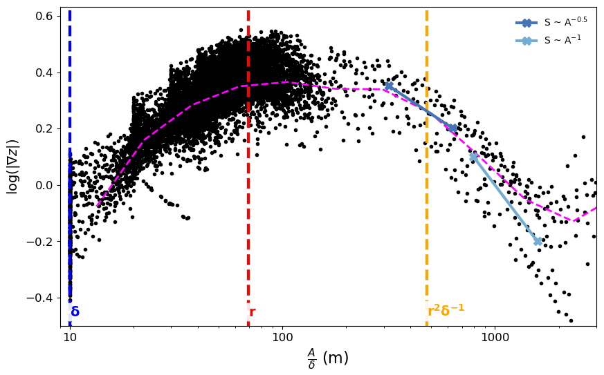
Figure 2 Slope-specific drainage area plot for the simulated topography shown in Fig. 3 for ℓ=1000 m, δ=10 m, $K=\mathrm{2.5}\times {\mathrm{10}}^{-\mathrm{5}}$ yr⁻¹, $D=\mathrm{7}\times {\mathrm{10}}^{-\mathrm{2}}$ m² yr⁻¹, and $U=\mathrm{3.6}\times {\mathrm{10}}^{-\mathrm{3}}$ m yr⁻¹. The binned median slope is plotted in magenta. The specific drainage area, a=r, shown with the red line, has the steepest slope. The specific drainage area value, $\frac{r^{\mathrm{2}}}{\mathit{\delta }}$, shown in orange, represents the transition to fluvial power-law scaling, with slope decreasing steadily with contributing area. This value is resolution-independent as an area but not as a specific drainage area, which has the fundamental dimension of length.

Larger values of $\frac{\mathrm{\ell }}{r}$ induce larger boundary sizes relative to r, therefore portraying more hillslopes and larger stream orders (Fig. 3). The dimensionless group $\frac{r}{\mathit{\delta }}$ controls the magnification (Fig. 4). Nodes with drainage area exceeding A=r² are shown with yellow dots. For different values of δ, the resolution changes, but the images stay largely the same.

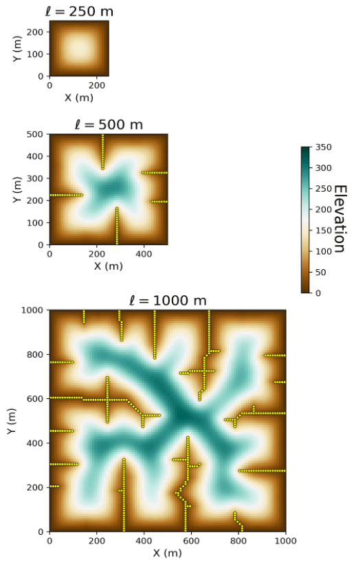
Figure 3 Computational simulation results varying ℓ for δ=10 m, $K=\mathrm{2.5}\times {\mathrm{10}}^{-\mathrm{5}}$ yr⁻¹, $D=\mathrm{7}\times {\mathrm{10}}^{-\mathrm{2}}$ m² yr⁻¹, and $U=\mathrm{3.6}\times {\mathrm{10}}^{-\mathrm{3}}$ m yr⁻¹. The corresponding channelization indices, $CI=\frac{{\mathrm{\ell }}^{\mathrm{2}}K}{D}$, are approximately 22, 89, and 357. These simulations preserve the dimensionless group $\frac{r}{\mathit{\delta }}$, the ratio of the characteristic length to the pixel width. Larger values of C_I, given the same r value, imply a resized boundary length, ℓ. Channels are highlighted with yellow dots for A≥r².

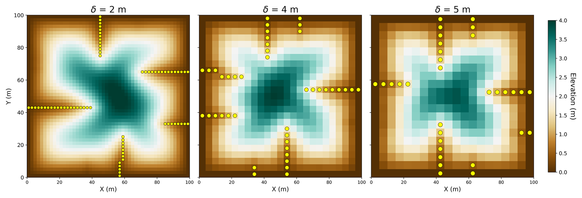
Figure 4 Computational results varying δ for $U=\mathrm{1}\times {\mathrm{10}}^{-\mathrm{3}}$ m yr⁻¹, $D=\mathrm{5}\times {\mathrm{10}}^{-\mathrm{2}}$ m² yr⁻¹, and $K=\mathrm{5}\times {\mathrm{10}}^{-\mathrm{4}}$ yr⁻¹. Nodes with drainage area exceeding $a=\frac{r^{\mathrm{2}}}{\mathit{\delta }}$ are shown with yellow dots. Varying δ with an $\frac{r}{\mathrm{\ell }}$ constant produces similar results. With decreasing $\frac{r}{\mathit{\delta }}$, maximum elevation decreases, since topographic maxima have a specific drainage area δ. This presents a possible benefit for subtracting δ from a, thus counting the number of links (Rodríguez‐Iturbe et al., 1997). We forgo this approach for simplicity.

4 Fractal analysis

In the steady-state simulations presented in Figs. 3 and 4, channel heads are located at $a\approx \frac{r^{\mathrm{2}}}{\mathit{\delta }}$. This value is well defined as an area, r², as hypothesized by Montgomery and Foufoula-Georgiou (1993), but not as a δ-derived specific drainage area.

On a discrete grid with pixel width δ, points with zero dimension have an area of δ², formed by a length and width of δ. Topographic maxima have zero-dimensional contributing drainage area, δ². On a two-dimensional mesh, lines are represented with a width equal to the grid resolution. Resolution-independent lengths on steady-state topography correspond to the inflection points, a=r, for linear diffusion. Using the D∞ algorithm, these lengths correspond to flow-routing lengths rather than to Euclidean lengths. The flow directions for nodes with a=r are locally parallel in ${lim}_{\mathit{\delta }\to \mathrm{0}}$, separating zones of topographic divergence (a<r) from topographic convergence (a>r). Areas on two-dimensional grids are resolution-independent. Numerical simulations (Figs. 3 and 4) indicate that these contributing areas correspond to nodes with A=r², such that the contributing area is convergent to a point, i.e., a channel head. In these simulations, according to Eq. (8), channels (linear elements which by definition have width δ) form downstream from these channel heads.

4.1 Fractal definition

The resolution-independent dimension of unchannelized nodes, with $a\le \frac{r^{\mathrm{2}}}{\mathit{\delta }}$, is not necessarily an integer. Nodes in locations with flow directions of partial convergence or partial divergence have non-integer, or fractal, dimension. The dimension of unchannelized nodes with integer dimension, using δ as a contour width, is

$$\begin{array}{}\text{(11)}& a={\displaystyle \frac{(r{)}^{D_{\mathrm{f}}}}{{\mathit{\delta }}^{D_{\mathrm{f}}-\mathrm{1}}}}.\end{array}$$

D_f is the box-counting fractal dimension, commonly defined as

$$D_{\mathrm{f}}={\displaystyle \frac{\log (\text{number of self-similar pieces)}}{\log (\text{magnification factor)}}}.$$

Solving for D_f,

$$\begin{array}{}\text{(12)}& D_{\mathrm{f}}={\displaystyle \frac{\log \left(\frac{a}{\mathit{\delta }}\right)}{\log \left(\frac{r}{\mathit{\delta }}\right)}}.\end{array}$$

The numerator, $\log \left(\frac{a}{\mathit{\delta }}\right)$, is the logarithm of the number of contributing pixels. The denominator, $\log \left(\frac{r}{\mathit{\delta }}\right)$, is the logarithm of the magnification factor, the dimensionless group $\frac{r}{\mathit{\delta }}$, referring to the number of contributing pixels at the inflection point. Therefore, for each node, Eq. (12) is calculated by comparing the logarithm of the number of contributing pixels to the logarithm of the number of pixels at the inflection point (Fig. 5). This fractal dimension is similar to definitions of Péclet numbers given in previous studies (Theodoratos et al., 2018; Hooshyar et al., 2020). Figure 6 shows the fractal dimension of the contributing drainage plotted for the parameters given in Fig. 2.

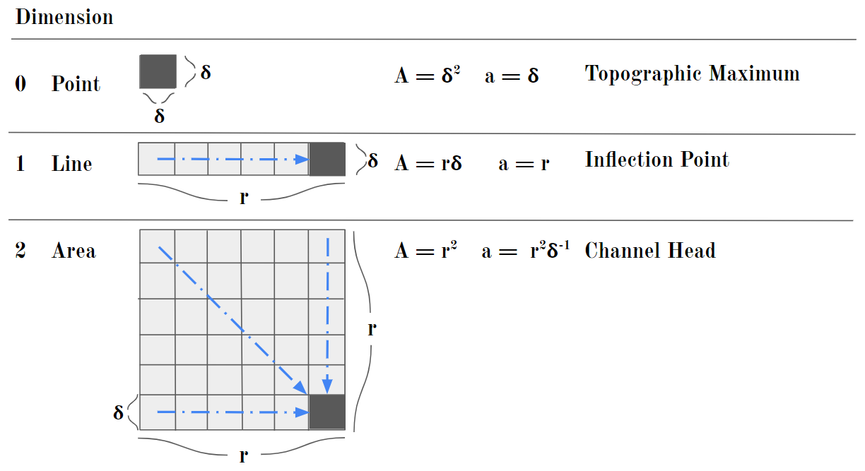
Figure 5 Schematic diagram of the non-fractal dimension drainage regions. On landscapes, lengths do not correspond to Euclidean lengths but correspond instead to flow lengths. Areas are not necessarily square-shaped.

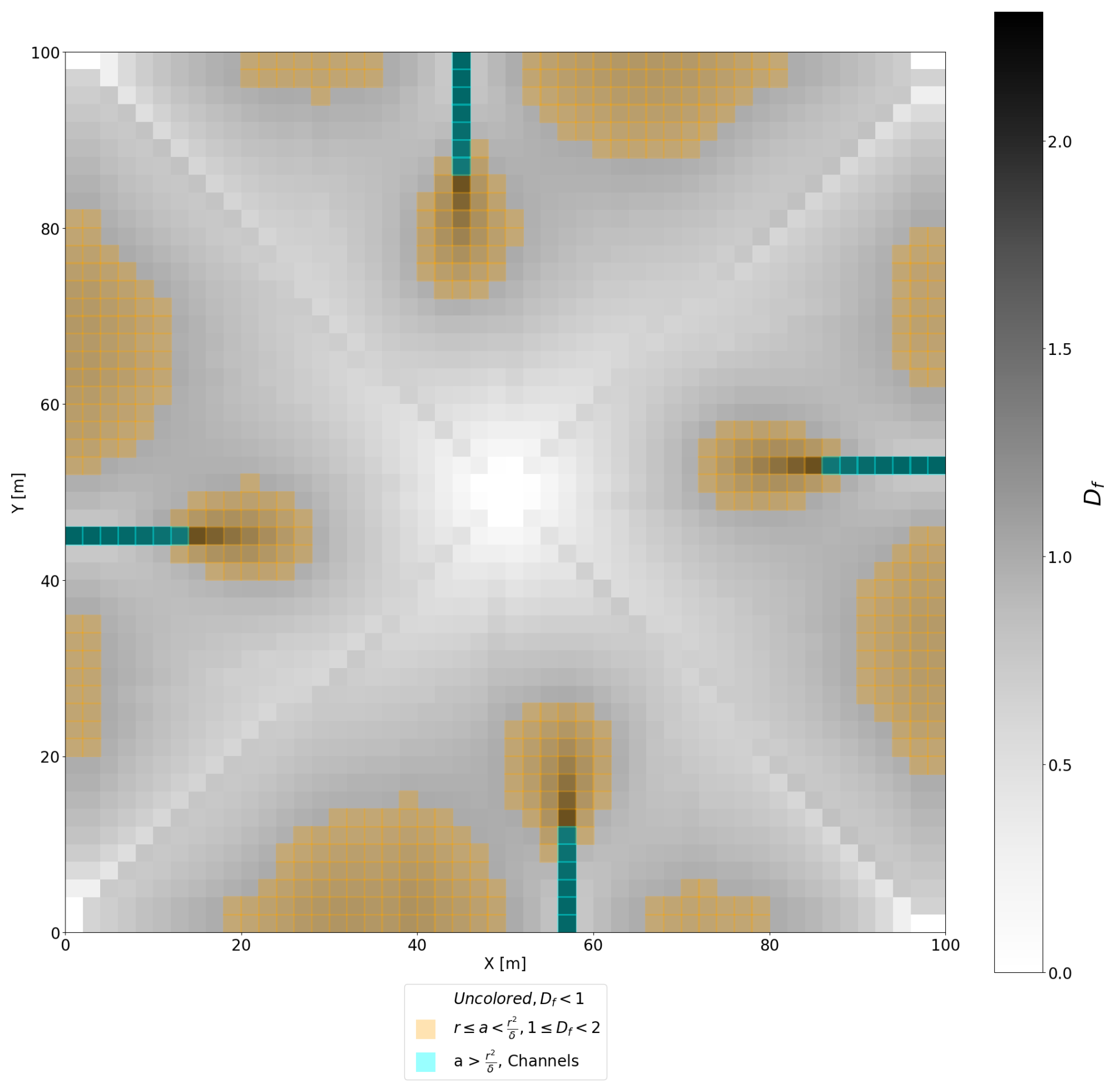
Figure 6 Simulation results for $U=\mathrm{1}\times {\mathrm{10}}^{-\mathrm{3}}$ m yr⁻¹, $D=\mathrm{5}\times {\mathrm{10}}^{-\mathrm{2}}$ m² yr⁻¹, $K=\mathrm{2.5}\times {\mathrm{10}}^{-\mathrm{4}}$ yr⁻¹, δ=2 m, and ℓ=100 m, plotted according to the fractal dimension, D_f (Eq. 12). Channel heads, with drainage area r², have dimension 2. Colluvial valleys correspond to $\mathrm{1}<D_{\mathrm{f}}<\mathrm{2}$. River segments have dimension 2 when accounting for channel width.

Equation (12) indicates that nodes with locally divergent flow near hilltops exhibit a contributing drainage region with fractal dimension between 0 and 1. Unchannelized nodes with locally convergent flow have a contributing drainage region with fractal dimension between 1 and 2, corresponding to unchannelized valleys (Fig. 6). This explanation clarifies the properties of unchannelized nodes but does not extend to channelized nodes.

Equation (12) suggests that, for channelized nodes, with $a\ge \frac{r^{\mathrm{2}}}{\mathit{\delta }}$, D_f exceeds 2 for a calculated using δ as a contour width. Several studies have demonstrated that the fractal dimension of channel networks, as measured by their length-to-bifurcation ratios, approaches 2 for large stream orders (Tarboton et al., 1988; Rinaldo et al., 1998; La Barbera and Rosso, 1989; Rodríguez‐Iturbe et al., 1997). While these fractal definitions may be independent, it would be unconventional for the box-counting fractal dimension of a region on a two-dimensional surface to exceed 2. For river segments observed in nature, channel width scales with the square root of drainage area (Leopold and Maddock, 1953). Letting δ be the channel width at the channel head,

$$\begin{array}{}\text{(13)}& w={\displaystyle \frac{\mathit{\delta }}{r}}\sqrt{A}.\end{array}$$

Box-counting with δ-sized pixels for river nodes downstream of the channel head captures only the contributing nodes for a fraction of the contour width of the channel. Using w as the contour width for river nodes, $A=a_w\cdot w$, where a_w is the specific contributing area corresponding to contour width w. Substituting a_w for a and w for δ in the numerator of D_f, as defined for hillslopes, D_f=2 for all channels. The ratio $\frac{r}{\mathit{\delta }}$ remains constant, the dimensionless magnification factor set by the parameters of the model.

$$\begin{array}{}\text{(14)}& w={\left({\displaystyle \frac{\mathit{\delta }}{r}}\right)}^{\mathrm{2}}\cdot a_w{D}_{\mathrm{f}}={\displaystyle \frac{\log \left(\frac{a_w}{w}\right)}{\log \left(\frac{r}{\mathit{\delta }}\right)}}\end{array}$$

5 Confirmation and discussion

To apply this theory to real-world landscapes suitable for the stream-power plus linear diffusion model, it is necessary to identify a set of hypotheses to test. Our first hypothesis is that the drainage area at the inflection point scales with 1 factor of grid resolution. Secondly, we hypothesize that the drainage area of channel heads is independent of grid resolution and corresponds to the square of the specific drainage area at the inflection point.

Gabilan Mesa is a frequent subject for studies of linear diffusion advection landscape evolution, featuring soil-mantled hillslopes with cohesive soils and uniform steady-state topography. Debris flows and shallow landsliding are uncommon. Gabilan Mesa also has low gradients in most places relative to the critical slope, supporting the assumption of linear diffusion (Perron et al., 2008, 2009). Our data originate from a 2015 DEM, as utilized by Grieve et al. (2016). These data include channel heads using the Pelletier algorithm (Pelletier, 2013), which estimates channel head locations from contour curvature. Floodplains were manually mapped and excluded. We did not need to run a sink-filling algorithm, since Gabilan features very little topographic roughness.

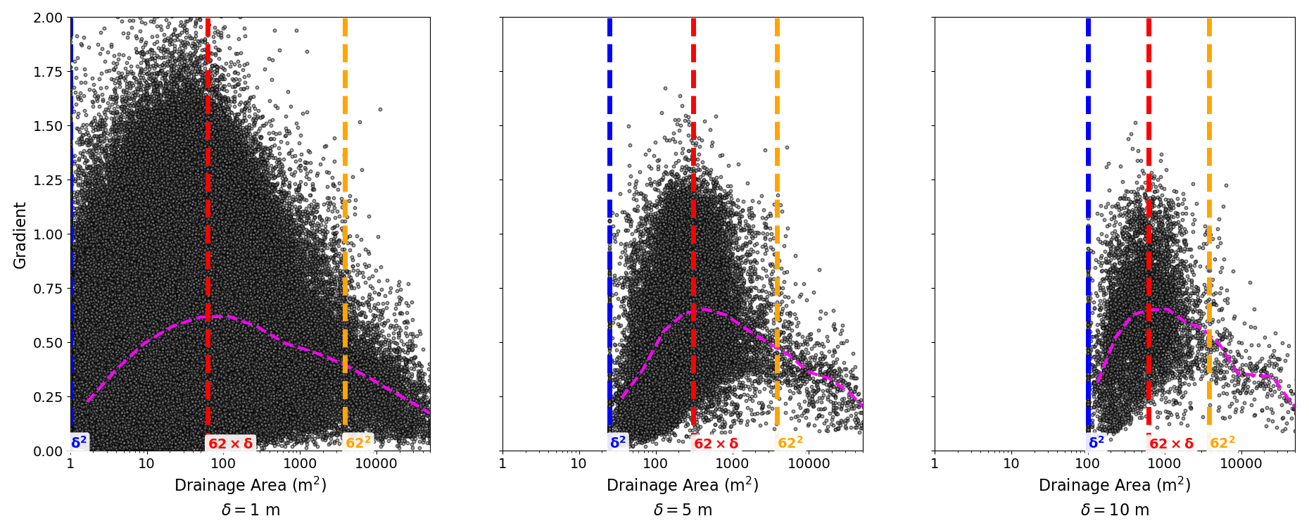
Figure 7 Log–log plot of slope by drainage area for Gabilan Mesa, resampled across 1, 5, and 10 m pixels, as shown in Fig. 8. The binned median is plotted with a dashed magenta line. The characteristic length is 62 m. The minimum drainage area, corresponding to topographic maxima, is δ². The drainage area of the inflection point is 62δm². Channel heads have the characteristic area of contributing drainage area which is resolution-independent.

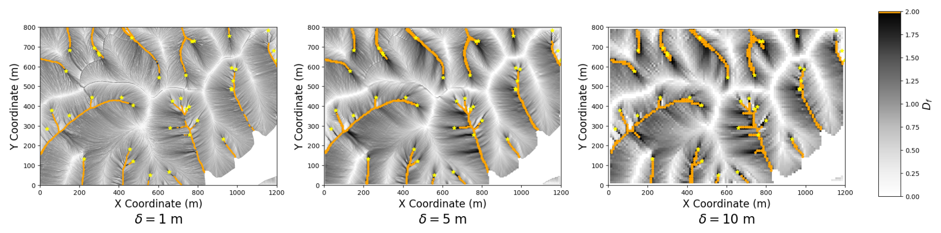
Figure 8 A section of Gabilan Mesa visualized by plotting the fractal dimension, D_f, for each node. Subsequent plots are generated by resampling the topographic elevation from the original 1 m DEM to 5 and 10 m resolution. The D∞ algorithm calculates flow accumulation for every pixel. The fractal dimension is calculated according to Eq. (12), using the characteristic length of 62 m, derived from Fig. 7. Channelized pixels, those with A>(62 m)² and thus a fractal dimension of greater than 2, are highlighted in orange. This algorithm is resolution-independent up to greater numerical error on coarser resolutions. Channel heads derived from the Pelletier algorithm (Pelletier, 2013) are marked with yellow stars, demonstrating a surprising correspondence between the channel head methods. Nodes with a fractal dimension of 1 separate regions of topographic divergence from topographic convergence.

Figure 7 plots the gradient by drainage area for the section of the DEM shown in Fig. 8. The characteristic length corresponding to the inflection point is 62 m, the drainage area of which varies by a factor of δ across resolutions (Bernard et al., 2022). Both Figs. 7 and 8 demonstrate that the drainage area of channel heads is resolution-independent, as predicted by Fig. 5 and Eq. (12). Figure 8 confirms that the location of channel heads, nodes with A=(62 m)² and thus D_f=2 with r=62 m in Eq. (12), matches the location of channel heads as identified by the contour curvature method of Pelletier (2013).

While D can be consistently defined by hilltop curvature, K is difficult to estimate from topography. Potential approaches include using drainage density (Tucker and Bras, 1998) or channel steepness (Whipple and Tucker, 1999). These approaches are problematic, since identifying K from channel steepness or drainage density would assume that erodibility is constant throughout the domain (both hillslopes and channel networks), which is unlikely given variations in sediment cover and physical processes. Another approach is outlined by Perron et al. (2009), who conducted a regression of $\frac{\left|\mathrm{\nabla }z\right|}{{\mathrm{\nabla }}^{\mathrm{2}}z-C_{\mathrm{ht}}}$, where C_ht is the hilltop curvature, against drainage area to derive values for $\frac{D}{K}$ and m, assuming a stream-power formulation with n=1 (Eq. 1). However, this analysis overlooks grid resolution, and, as demonstrated in Fig. 7, drainage areas on hillslopes are not independent of grid resolution. Consequently, this regression is not a valid method for extracting m and $\frac{D}{K}$.

Given the consistency between our numerical simulations and the topography of Gabilan Mesa, we consider it likely that $r=\mathrm{1.3}\sqrt{\frac{D}{K}}\approx \mathrm{62}$ m for this case study, though we leave rigorous validation of these parameters, K in particular, for future work. Nonetheless, the coherence between the topographic analyses presented in Figs. 7 and 8 and the mathematical framework derived from computational results confirms the utility of our theory (Bras et al., 2003).

5.1 Spatially resolving channel width

The numerical simulations shown in this paper correspond to Eq. (8), with specific area calculated with contour width δ. These simulations have channel slopes that scale according to a concavity of $\frac{m}{n}=\mathrm{1}$, rather than a concavity of $\frac{m}{n}=\frac{\mathrm{1}}{\mathrm{2}}$, because the scaling in channel width is confined to a single pixel. Previous approaches, as given by Pelletier (2010), assume that pixel widths exceed channel widths throughout the simulated domain, such that pixel elevations represent the channel elevation within the pixel rather than the average elevation. This results in the form $\frac{A}{w}$, where w is the channel width (Eq. 14), such that channel slope scales with drainage area according to the exponent $m=\mathrm{1}-\mathit{\alpha }$, where α is the scaling of channel width (Pelletier, 2010). For self-similarity given Eq. (14), $\mathit{\alpha }=\frac{\mathrm{1}}{\mathrm{2}}$; thus channels scale with drainage area according to $m=\frac{\mathrm{1}}{\mathrm{2}}$. However, applying $\frac{A}{w}$ to a single pixel forgoes the spatial representation of widening channels. Rather than assuming that pixel widths exceed channel widths throughout the domain, we propose instead that models should assume that channel widths exceed the pixel width, with the pixel width equal to the channel head width, as suggested by Litwin et al. (2022b). With this assumption, flow-partitioning across multiple pixels could accommodate widening channels (Gailleton et al., 2024), enabling the precise depiction of river longitudinal profiles and widths.

5.2 Arbitrary $\frac{r}{\mathit{\delta }}$

For large δ relative to r, landscapes are largely self-similar (Anand et al., 2023; Hergarten, 2020), with concave-down hillslope profiles restricted to single pixels. These simulations converge to purely fluvial topography for $\frac{r}{\mathit{\delta }}\to \mathrm{0}$, with channel-scaling behavior occurring instantly. Likewise, previous works regarded δ as an arbitrary value, seeking relationships to vary between δ (Pelletier, 2010). We suggest no such abstraction to vary between δ for numerical simulations. Real-world landscapes typically feature r≫δ, introducing computational challenges that can be mitigated by choosing a small $\frac{\mathrm{\ell }}{r}$.

5.3 Physical merit to δ

In computational models, the channel head, with upstream contributing drainage r², marks the beginning of channels, linear elements of width δ. In ${lim}_{\mathit{\delta }\to \mathrm{0}}$, channel heads are points, resulting in precisely linear channels regardless of the area-scaling. This is not the behavior observed in nature. In ${lim}_{\mathit{\delta }\to \mathrm{0}}$, the topography of steady-state computational simulations minimizes numerical error to form a smooth surface, whereas real-world landscapes feature roughness at increasingly small scales (Roering, 2008). This indicates the importance of other length scales in real-world landscapes, including the particle size (Andrle and Abrahams, 1989; Sangireddy et al., 2017; Sweeney et al., 2015; Dunne and Jerolmack, 2020), which are omitted from one-dimensional analyses. Studies have shown that the particle size distribution is closely related to the transition from slope-invariant colluvial valleys (i.e., $\mathrm{1}<D_{\mathrm{f}}<\mathrm{2}$) and fluvial channels, suggesting a maximum particle size at the channel head (Neely and DiBiase, 2023).

5.4 Nonlinear diffusion

Physical landscapes are influenced by a variety of processes not explicitly considered in this analysis, such as soil production (Heimsath et al., 1997), nonlinear diffusion (Roering et al., 1999), and groundwater infiltration (Litwin et al., 2022b). The fractal dimension of drainage region is a result of convergence and divergence on topography and is not inherent to the one-dimensional equation with linear diffusion. Future work should seek to generalize this work to a variety of flux laws, such as nonlinear diffusion law in the Andrews–Bucknam form (Roering et al., 1999; Andrews and Bucknam, 1987), depth-dependent nonlinear diffusion (Roering, 2008), and nonlocal models (Foufoula-Georgiou et al., 2010; Furbish and Roering, 2013). For nonlinear diffusion in the form of Roering et al. (1999) and Andrews and Bucknam (1987), the characteristic length is not proportional to $\sqrt{\frac{D}{K}}$ but is also a function of uplift relative to the critical slope. Identifying the characteristic length from topography with strongly nonlinear diffusion is inherently challenging, as hillslopes nearing the critical slope become planar (Roering et al., 2007). Additionally, computational models incorporating nonlinear diffusion must address the nonlinear effects of the grid resolution setting the spatial scale of the diffusion process (Ganti et al., 2012; Furbish and Roering, 2013).

5.5 Curved slope–area plots

The reasons for curved slope–area plots have long been a topic of discussion in geomorphology (Montgomery and Foufoula-Georgiou, 1993). Colluvial valleys, corresponding to the curved region between hillslopes and channels in slope–area plots, have often been attributed to the role of stochastic processes, such as debris flows and shallow landslides. We showed that, for these regions, drainage area is not a reliable metric. For analyses of natural landscapes, our theory should help elucidate the role of debris flows and landslides (McGuire et al., 2023). For computational simulations, this intuition shows potential for testing theories related to the frequency of forcing, both tectonic and climatic, in hillslope–channel-coupled landscape evolution (Godard and Tucker, 2021).

6 Conclusions

We showed that the relationship between the characteristic landscape length and grid resolution in the stream-power plus linear diffusion landscape evolution model is expressed as a multifractal system for unchannelized nodes. Nodes with locally divergent flow have a contributing drainage region with fractal dimension between 0 and 1, while unchannelized nodes with locally convergent flow display dimensions between 1 and 2, aligning with unchannelized valleys. Channels have a well-defined contributing area, aligning with the observed scaling of channel width and channel slopes as the square root of drainage area. This finding underscores a significant parallel between computational grid resolution and real-world landscape features – the channel head and particle width, in particular. This study serves as a foundational step towards understanding geomorphic channel–hillslope coupling, highlighting the coherence and limitations of one-dimensional and two-dimensional landscape evolution equations.

Appendix A: Alternate derivation of r

Let $y=\frac{\mathrm{d}z}{\mathrm{d}x}$, $y^{\prime }=\frac{{\mathrm{d}}^{\mathrm{2}}z}{\mathrm{d}{x}^{\mathrm{2}}}$. Let $x\ge \mathrm{0},y\le \mathrm{0}$, by symmetry. Then, rearranging Eq. (2), we have the form of a first-order linear ODE in y, which can be solved by the integrating factor method.

$$\begin{array}{}\text{(A1)}& {\displaystyle }{y}^{\prime }+{\displaystyle \frac{K}{D}}xy=-{\displaystyle \frac{U}{D}},\text{(A2)}& {\displaystyle }\mathit{\mu }\left(x\right)=e^{\frac{K}{\mathrm{2}D}{x}^{\mathrm{2}}},\text{(A3)}& {\displaystyle }y=-{\displaystyle \frac{U}{D}}{e}^{-K{x}^{\mathrm{2}}/\mathrm{2}D}\underset{\mathrm{0}}{\overset{x}{\int }}{e}^{\frac{K}{\mathrm{2}D}{\stackrel{\mathrm{‾}}{x}}^{\mathrm{2}}}\mathrm{d}\stackrel{\mathrm{‾}}{x}+C.\end{array}$$

Using y(0)=0,

$$\begin{array}{}\text{(A4)}& y=-{\displaystyle \frac{U}{D}}{e}^{-K{x}^{\mathrm{2}}/\mathrm{2}D}\underset{\mathrm{0}}{\overset{x}{\int }}{e}^{\frac{K}{\mathrm{2}D}{\stackrel{\mathrm{‾}}{x}}^{\mathrm{2}}}\mathrm{d}\stackrel{\mathrm{‾}}{x}.\end{array}$$

Using $y=\frac{U}{Kx}$, the characteristic length can be solved for using a series-expansion and a root-finding algorithm.