AI-based tracking of fast-moving alpine landforms using high-frequency monoscopic time-lapse imagery

Active rock glaciers and landslides are dynamic landforms in high mountain environments, where their geomorphic activity can pose significant hazards, especially in densely populated regions such as the European Alps. Moreover, active rock glaciers reflect the long-term thermal state of permafrost and respond sensitively to climate change. Traditional monitoring methods, such as in situ differential Global Navigation Satellite System (GNSS) and georeferenced total station (TS) measurements, face challenges in measuring the rapid movements of these landforms due to environmental constraints and limited spatial coverage. Remote sensing techniques offer improved spatial resolution but often lack the necessary temporal resolution to capture sub-seasonal variations. In this study, we introduce a novel approach utilising monoscopic time-lapse image sequences and artificial intelligence (AI) for high-temporal-resolution velocity estimation, applied to two subsets of time-lapse datasets capturing a fast-moving landslide and rock glacier at the Grabengufer site (Swiss Alps). Specifically, we employed the Persistent Independent Particle tracker (PIPs$++)$ model for 2D image point tracking and the image-to-geometry registration to transfer the measured 2D image points into 3D object space and further into velocity data. For the latter, we use an in-house tool called GIRAFFE, which employs the AI-based LightGlue matching algorithm. This methodology was validated against GNSS and TS surveys, demonstrating its capability to provide spatially and temporally detailed velocity information. Our findings highlight the potential of image-driven methodologies to enhance the understanding of dynamic landform processes, revealing spatiotemporal patterns previously unattainable with conventional monitoring techniques. By leveraging existing time-lapse data, our method offers a cost-effective solution for monitoring various geohazards, from rock glaciers to landslides, with implications for enhancing alpine safety. This study marks the pioneering application of AI-based methodologies in environmental monitoring using time-lapse image data, promising advancements in both research and practical applications within geomorphic studies.

1 Introduction

Active rock glaciers are creeping permafrost features (Barsch, 1996; Kääb and Reichmuth, 2005), serving as indicators of permafrost distribution in high mountain environments (Marcer et al., 2017; RGIK, 2023). Their velocity results from various parameters, such as topographic conditions, rock glacier material, and internal structure, and it reflects long-term, temperature-driven changes in permafrost structure (Cicoira et al., 2021; Delaloye et al., 2010). Higher creep rates typically occur towards the lower permafrost limits, where mean annual air temperatures approach 0 °C (Frauenfelder et al., 2003). They efficiently transport sediment (Delaloye et al., 2010; Kummert and Delaloye, 2018), and this becomes more pronounced as rock glacier creep rates increase in a warming climate (Delaloye et al., 2013; Pellet et al., 2023). Similarly, large volumes of sediment can be mobilised by permafrost-affected rock slope failures, such as deep-seated slides, topples, or deformations that involve in situ bedrock (McColl and Draebing, 2019). This can pose significant geohazards when direct connections to downslope infrastructure exist. Precise monitoring of these fast-moving high-alpine landforms is thus essential for future alpine safety (Hermle et al., 2022), as it provides information about the environmental drivers and enhances process understanding.

The monitoring of fast-creeping rock glaciers (>3 m a⁻¹, Marcer et al., 2021) or landslides is particularly challenging. Traditional techniques that require frequent field access, such as in situ differential Global Navigation Satellite System (GNSS) measurements, face environmental and logistical obstacles. Permanent GNSS installations can offer displacement observations with millimetre accuracy at a continuous temporal resolution, but they may not have the desired longevity on fast-moving landforms due to extreme cases of block sliding, rotation, and rockfall, necessitating re-levelling or instrument replacement (Cicoira et al., 2022). Both GNSS and total station (TS) measurements only measure discrete points, resulting in a limited spatial distribution. However, spatial heterogeneity of landform movement can be expected depending on internal rock glacier structure and terrain characteristics (RGIK, 2023). Improved spatial coverage can be achieved using remote sensing data, such as 3D point clouds derived from uncrewed aerial vehicles (UAVs) and terrestrial or airborne laser scanning (TLS or ALS). These techniques minimise the need for extensive field access, enabling operators to avoid in-person exposure to the fastest-moving areas while still capturing detailed data from these regions. However, these methods often lack the temporal resolution necessary to capture sub-seasonal variations in the landform to its environmental drivers, essential to increase process understanding. Time-lapse imagery or webcam data have the capability to capture the kinematics of alpine landforms with e.g. hourly resolution. Fixed photogrammetric camera systems, which are increasingly implemented, involve multiple time-lapse cameras to reconstruct high-resolution 3D point clouds similar to those from UAVs or TLS and at a fraction of the cost (Blanch et al., 2023; Eltner et al., 2017; Ioli et al., 2024; Ulm et al., 2025). Nonetheless, deploying multiple cameras in dynamic alpine environments can be challenging, often requiring wide baselines that complicate point cloud generation (Ioli et al., 2024). Recent studies have demonstrated that metric measurements can be obtained from 2D images alone when a 3D model is available, reducing the need for extensive camera arrays (Altmann et al., 2020; Elias et al., 2023; Wegner et al., 2023). Furthermore, monoscopic camera data, which are more readily available than stereo images, often span 1 decade or more in the European Alps (Kummert et al., 2018). Generally installed in stable terrain, these cameras tend to have greater longevity than permanent GNSS installations. However, most time-lapse camera systems are highly weather-dependent. Changes in the camera's intrinsic and extrinsic properties caused by thermal variations (e.g. Elias et al., 2020) and external disturbances such as snow and wind are common, significantly affecting the image configuration. Additionally, maintaining a perfectly stable camera position over the long term can be very challenging in a dynamic mountain environment.

Measuring the velocity of boulders in the camera's field of view is possible by measuring homologous point correspondences between images in a series, a common challenge in computer vision called feature tracking using optical flow-based methods and feature matching (Fortun et al., 2015). Feature tracking is essentially an optimisation problem, where the location of highest similarity between a reference template and a template in the destination image is considered a match (Eltner et al., 2022). Common similarity measures include normalised cross-correlation (NCC) (Heid and Kääb, 2012) and least squares matching (LSM; Schwalbe and Maas, 2017). While traditional motion estimation methods are commonly applied in natural hazard management, they face decorrelation challenges with large displacements, strong illumination changes, and occlusions. Image pre-selection is crucial to minimise illumination variations (e.g. selecting images from the same time of day), thereby limiting temporal resolution (How et al., 2020). In the era of artificial intelligence (AI), traditional feature tracking can leverage the power of deep learning. Convolutional neural networks (CNNs), employed as feature extractors, replace handcrafted features or the use of image intensities or gradients (Hur and Roth, 2020). This approach offers the advantage of representing each pixel with a high-dimensional feature vector, blending distinctiveness and invariance to, for example, appearance changes, thereby improving feature robustness over time. This enhances, on the one hand, image feature tracking (e.g. Persistent Independent Particle tracker (PIPs$++$; Zheng et al., 2023), VideoFlow (Shi et al., 2023), Raft (Teed and Deng, 2020)) and, on the other hand, image matching algorithms, as seen with models such as SuperGlue (Sarlin et al., 2020), LightGlue (Lindenberger et al., 2023), or LoFTR (Sun et al., 2021).

This study aims to derive high-resolution spatiotemporal landform velocities from monoscopic time-lapse cameras, verified through permanent in situ GNSS and TS surveys. We tested the deep learning model called Persistent Independent Particle tracker (PIPs$++)$ (Harley et al., 2022; Zheng et al., 2023) to track landslide and rock glacier movements and the AI-based image matcher LightGlue (Lindenberger et al., 2023) for 2D-to-3D registration. This process is implemented in our in-house, open-source tool, Geospatial Image Registration And reFErencing (GIRAFFE), which renders synthetic images from scaled 3D point clouds and estimates a linear camera model to match the 2D image perspective. Originally introduced by Elias et al. (2019) for water level monitoring using SIFT (Lowe, 2004), GIRAFFE was later improved with the AI-based SuperGlue matcher (Sarlin et al., 2020) for multi-modal image-to-geometry registration (Elias and Maas, 2022; Elias et al., 2023). In this study, we use the stable and open-source LightGlue matcher and release the GIRAFFE source code to support flexible, time-lapse-based velocity analysis. We introduce a novel low-cost image-based remote measurement technology designed for challenging and hard-to-access terrains. The proposed method has been validated for two time-lapse image datasets by extracting image-based velocity information. Two rapidly moving alpine landforms, a landslide and a rock glacier, were observed at the Grabengufer site in Switzerland (Kenner et al., 2014). We highlight the potential of our methodology to manage large datasets effectively and enhance the spatiotemporal understanding of landform dynamics. Our approach not only improves analytical capabilities but also facilitates the use of basic systems, such as monoscopic cameras, for automated, cost-effective monitoring and quantification of landform movements.

2 Study area

The Grabengufer study area features two fast-moving alpine landforms (Fig. 1a). The upper section (2700–2880 m a.s.l.) consists of an extensive deep-seated landslide moving up to 1.5 m a⁻¹ (Fig. 1a, blue polygon). According to installed ground surface temperature (GST) loggers, its mean annual surface temperature is still below 0° despite recent warming. The southern part of the landslide is frozen and ice-saturated (unpublished geophysical data and local inspection of fresh scars after rockfalls). Maximal intra-annual velocities are reached around November, and the velocities multiplied by 4 (from 0.3 to 1.2 m a⁻¹) between 2009 and 2024. However, due to the absence of rock glacier morphology and the uncertainty of driving factors for the landform's motion, we use the generic term “landslide”. The frontal section of the southern part of this landslide is highly unstable and a frequent source of rockfalls. Downslope, it gradually transitions into a zone of very rapid mass movement, referred to as the “(rock glacier) feeding section”. The transition between these two areas is gradual, without a clear boundary: the frontal section marks the upper part of the landslide, where debris of various sizes detach, while the feeding section moves significantly faster and shows no further detachment. Both areas are monitored by a permanently installed webcam (hereinafter Wcam04; Fig. 1c, orange polygon). For the purpose of this study, and to simplify terminology, we do not distinguish between the two in the analysis and refer to them collectively as the “frontal feeding section”. The fed rock glacier (2400–2600 m a.s.l., Wcam05; Fig. 1b, red polygon) is very active and was considered destabilised during the 1940s and 2000s (Delaloye et al., 2013). As of summer 2023, in situ measurements indicate that it has again been moving exceptionally fast at a rate of 91 to 255 m a⁻¹ (0.25 to 0.70 m d⁻¹), marking a third phase of destabilisation. The rock glacier tongue terminates on a very steep slope section leading into a gully prone to debris flows, which is observed by a separate webcam not included in this study.

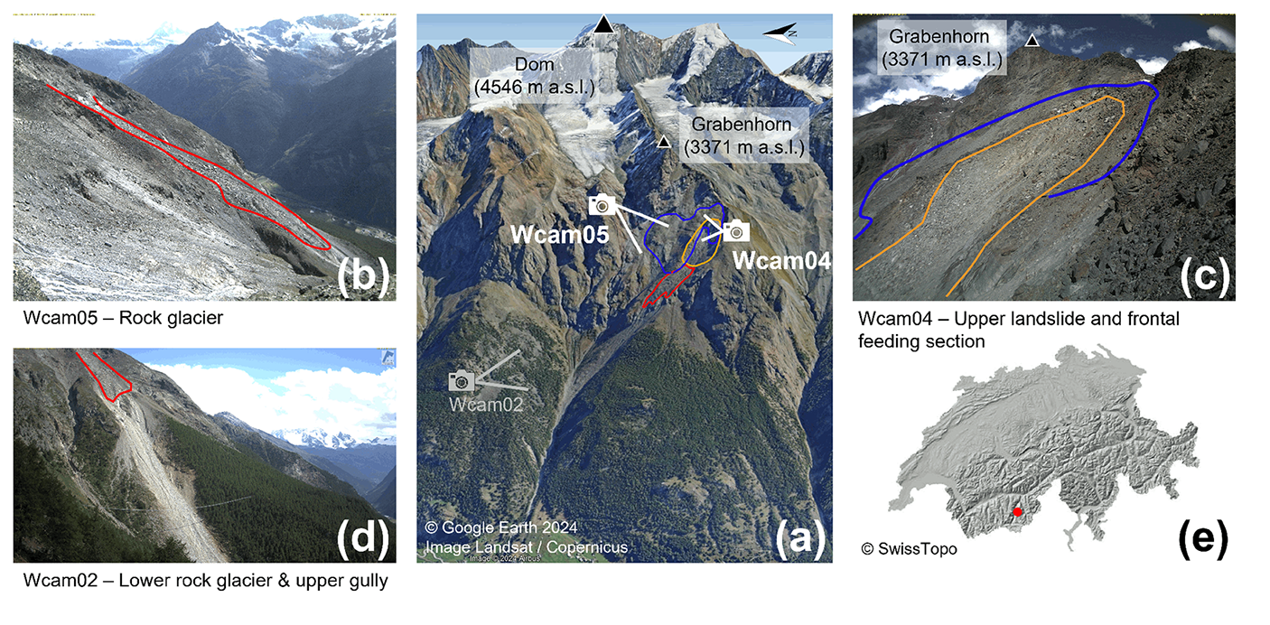
Figure 1 Overview of the Grabengufer study area in the Mattertal, Swiss Alps. (a) The locations of the webcams and the extent of the studied landforms: the landslide (blue), the frontal feeding section (orange), and the rock glacier (red). (b) Example image from webcam Wcam05, capturing the rock glacier. (c) View from webcam Wcam04, focused on the frontal section of the landslide that gradually feeds into the rock glacier – referred to as the frontal feeding section in this study. (d) Image from webcam Wcam02, which covers a lower portion of the rock glacier and an adjacent upper gully; this webcam was not used in the present study. (e) Geographic location of the study area within southwestern Switzerland.

3 Dataset description

The site is extensively monitored through bi-annual differential GNSS surveys (conducted at the end of June and October), several permanent GNSS installations operated by PermaSense (Cicoira et al., 2022) and Canton of Valais, 10 fixed reflectors for repeated TS measurements (approximately once a month), three time-lapse cameras operational since 2010/2013 (Wcam02, Wcam04, and Wcam05), and three GST loggers. For this study, we used the monthly TS measurements and a permanent GNSS installed and operated by the Canton of Valais (providing continuous data saved as 2 h means) to validate the velocities derived from the time-lapse image sequences. This GNSS uses a local fixed reference station in stable terrain located approximately 3 km away and 250 m lower in elevation, to provide accurate differential positioning. The image data analysed in this study were captured by the webcams Wcam04 and Wcam05, powered by solar panels. The characteristics of these webcams are summarised in Table 1.

The 3D reference data utilised for image-to-geometry registration were derived from UAV parallel-axis nadir image flights conducted using a DJI Phantom 4 RTK. These flights were performed on 3 July and 22 July 2023 to reference images from Wcam04 and Wcam05, respectively. The 3 July dataset consists of 1000 images captured at 85 m above ground level, yielding a 2.5 cm ground sampling distance (GSD). Four ground control points (GCPs) were used for georeferencing, with positional errors of 1 cm horizontally and vertically. The challenging terrain limited the inclusion of additional checkpoints. The 22 July dataset covers a larger area, extending to the valley, with 1800 images taken at 88 m altitude, maintaining a similar GSD. Seven GCPs were distributed across the site, with two independent checkpoints. GCP residual errors averaged 4 cm, while checkpoint errors were higher (7.5 cm horizontal, 9.5 cm vertical). The georeferencing of these 3D point clouds employed an integrated approach, combining RTK measurements of image position and onboard IMU data. The image blocks were processed using Structure-from-Motion Multiview Stereo (SfM-MVS) techniques implemented in Agisoft Metashape v.1.7, resulting in high-resolution 3D point clouds enriched with RGB colour information. Additional GCPs were used to ensure a stable configuration (e.g. Elias et al., 2024). The resulting 3D point clouds were resampled to a point spacing of 5 cm. This resampling facilitated the management of the large volume of 3D data, comprising hundreds of millions of points, while preserving detailed topographic representation.

Table 1 Camera and image dataset specifications.

¹ CH1903+ is a commonly used Swiss coordinate system. ² GSD: ground sampling distance. Size of the pixel on the landform of interest.

4 Methods

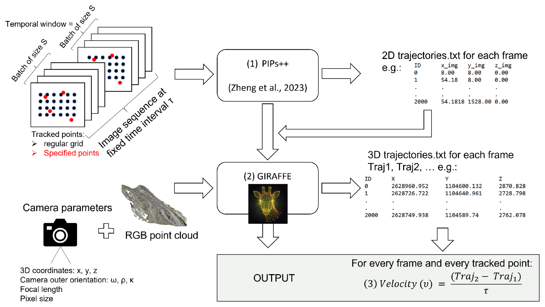
The workflow, visualised in Fig. 2, consists of two main steps designed to efficiently and accurately derive 3D trajectories from time-lapse image sequences. Firstly (1), translation vectors (pixel-based trajectories) for predefined tracking points, either arranged on a regular grid or at specified pixel coordinates, are extracted from the image sequence. In the next step (2), these 2D trajectories, estimated between consecutive images, are mapped to real-world coordinates using a 3D point cloud of the region of interest, which defines the reference system (see Fig. 2). This transformation enables the calculation of 3D coordinates for the tracked points to generate 3D trajectories. Finally, these trajectories are used to compute velocities, with units determined by the temporal resolution of the input data, such as the time-lapse interval (e.g. m d⁻¹).

The primary requirement of our workflow is a set of time-lapse images from fixed or otherwise stabilised cameras, preferably captured at consistent intervals (e.g. hourly, daily, or weekly) with date and time information embedded in the filenames. Additionally, approximate values for the camera pose and intrinsic parameters, such as focal length and pixel size, are necessary.

Figure 2 Schematic overview of the workflow presented in this study.

4.1 Application of the Persistent Independent Particle tracker (PIPs$++)$

The first step in our workflow involves feeding the image sequence into the Persistent Independent Particle tracker (PIPs$++$). The AI-based tracker, developed by Harley et al. (2022) and improved by Zheng et al. (2023), operates without retraining on our specific data. PIPs$++$ operates as a low-level tracker, relying on appearance-matching cues just like traditional methods (Eltner et al., 2020) but leveraging the full information that is available from the image sequence within the temporal window. It employs a 2D residual CNN for feature extraction in the initial step (He et al., 2016), generating a feature map for each frame independently of the image before or after. Following feature extraction, the algorithm feeds into a deep 1D CNN (ResNet) with fixed-length kernels applied to arbitrary temporal spans (Zheng et al., 2023). PIPs$++$ calculates descriptors and then estimates the local similarity of each feature to match them over time. Using spatial pyramids, it iteratively refines the position of these matched features, similarly to the RAFT model (Teed and Deng, 2020). Correlation matrices are calculated to align the feature templates as in already established approaches. PIPs$++$ operates within a multi-frame temporal context, considering all frames in a temporal window or batch of size S to search for the target. After a match is found, the trajectory of the feature within the batch is updated with one position per frame, resulting in a single continuous trajectory per batch for that feature. The correlation matrices are recalculated iteratively to refine the tracking process. If tracking fails in one frame due to occlusion (e.g. fog), the trajectory of the feature can still be estimated by interpolating the position, provided that the feature reappears in subsequent frames within the batch (as long as the fog does not last longer than the batch size S; see Fig. 3b). To increase robustness, the model computes similarity using multiple templates per feature. This means that the model not only relies on the feature's initial appearance in the first frame but adapts to changes in appearance along the trajectory, i.e. throughout the sequence. If the feature's appearance changes, due to snow cover (Fig. 3d), lighting shifts, or rotation, the model can update templates along the trajectory, storing multiple representations (templates) for the same feature. This multi-template approach allows tracking to continue even with appearance variations caused by environmental factors such light changes, snow cover, or self-occlusion (e.g. rolling boulders). Thus, the model handles appearance changes flexibly and tracks the feature over time using these multiple templates. The output of the model is a simple trajectory .txt file per frame (see Fig. 2, lower right), with the pixel coordinates of each tracked point. This file can be visualised on the respective image for visual inspection (Fig. 3). If a regular grid is used, it is reset each time a new batch starts.

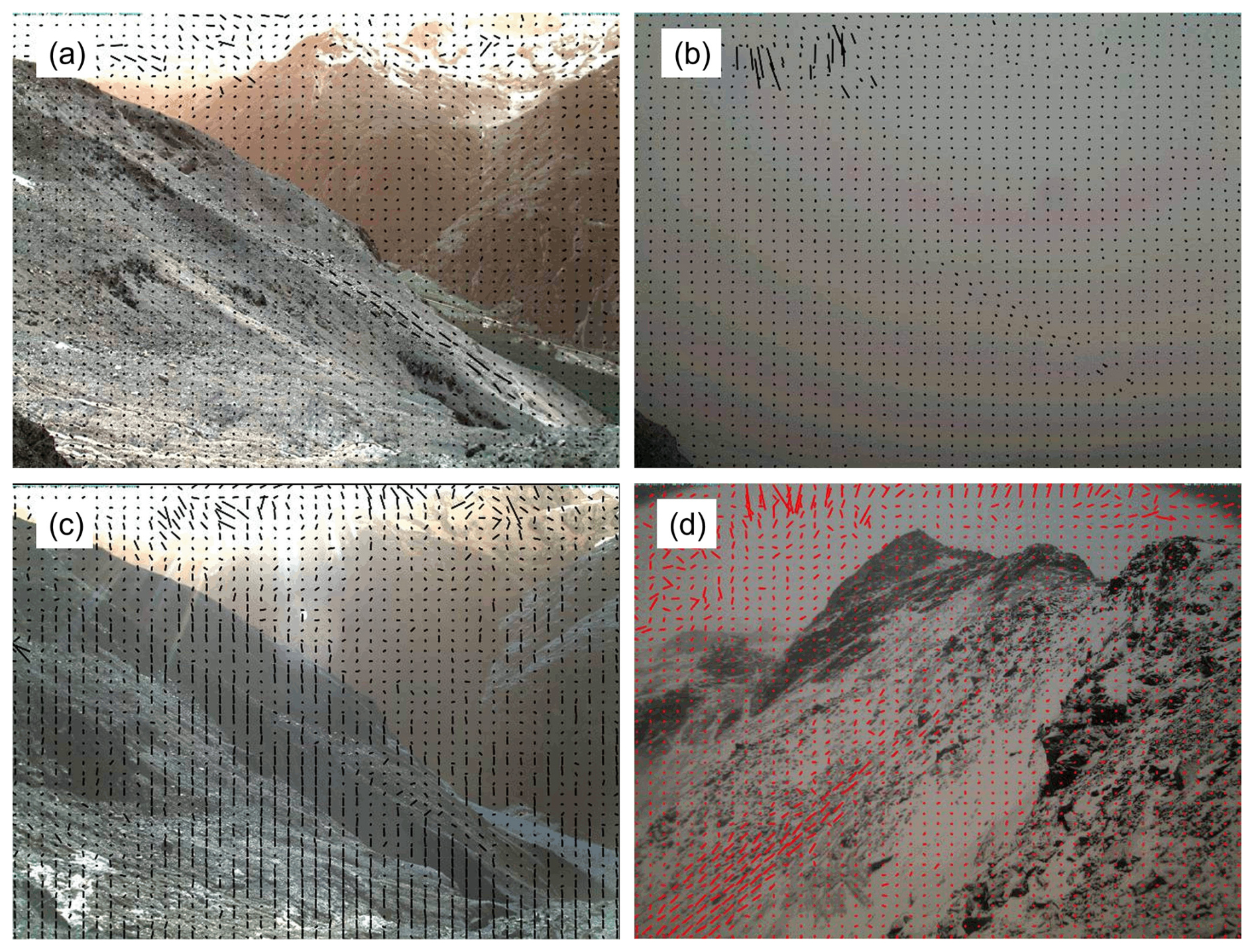
Figure 3 Some examples of velocity vectors as output from the PIPs$++$ model. (a) View of Wcam05, clearly identifying the moving rock glacier body despite its suboptimal viewing angle. (b) Same view occluded by fog, but tracking is interfered from the image before and after. (c) Same view displaying a systematic shift in the stable areas due to camera movement. (d) View of Wcam04 proving the good performance of PIPs$++$ in varying snow conditions.

4.2 From 2D to 3D: image-to-geometry registration using GIRAFFE

Image-to-geometry registration in GIRAFFE aligns 2D images with a photorealistic synthetic image rendered from a 3D point cloud. This process enables the transfer of 2D image data into 3D object space by estimating the camera's pose within the point cloud's coordinate system. This subsection aims to give a brief overview of the processing steps done in GIRAFFE; for more details, refer to the code documentation on GitHub.

4.2.1 Synthetic image generation

A synthetic image is rendered from an RGB-coloured 3D point cloud using an initial estimate of the camera's focal length and pixel size. The rendering simulates the real camera perspective while preserving spatial information from the 3D point cloud.

During the process, 3D points are projected onto a virtual image plane using a linear pinhole camera model. Frustum culling defines the view frustum (illustrated in Fig. 4), while a k-nearest neighbour (kNN) approach addresses gaps – when no points fall into a pixel – through radiometric gap-filling. Note that, in computer graphics, a frustum is the 3D volume visible through a camera or perspective projection, shaped like a pyramid with its top cut off, bounded by near and far clipping planes. Though these gap-filled pixels lack actual 3D information, they assist in subsequent image matching between the real and synthetic image. Once the synthetic image is generated, it provides a photorealistic depiction of the 3D point cloud, matching approximately the perspective of the original true camera image and retaining the original 3D information.

4.2.2 Image matching and camera pose estimation

Using LightGlue (Lindenberger et al., 2023), homologous points between the real and synthetic image are identified and matched, resulting in a list of corresponding 2D–3D image coordinates. Thereby, a kNN approach is applied to the synthetic image to find, for each image coordinate, the nearest valid 3D point, using a default maximum distance of 2.5 pixels.

These correspondences act as pseudo-control points to determine the camera pose and intrinsic parameters via an extended space resection approach, formulated as a perspective-n-point (PnP) problem. Optimisation is performed using the Levenberg–Marquardt algorithm (implemented in OpenCV v4.10). If the spatial distribution of control points is sufficient, lens distortion parameters can also be estimated; otherwise, distortion is neglected.

4.2.3 Accuracy considerations

The accuracy of image-to-geometry registration depends on the following:

• Point cloud quality. Higher density and accuracy improve precision in space resection.

• Spatial distribution of matches. Uniformly distributed 2D–3D correspondences across the whole image enhance model stability, while poorly distributed points (e.g. along collinear alignments) can degrade results.

• Distance threshold for matching. A lower threshold (here set to 2.5 pixels) improves precision but reduces the number of valid matches, affecting robustness.

An automatic distribution control mechanism implemented in GIRAFFE ensures an adequate pseudo-control point configuration before estimating non-linear camera models. To achieve this, the image is divided into quadrants, ensuring a balanced distribution of pseudo-control points across the image domain. Striking an appropriate balance between precision and the density of control points is also essential for optimising the overall calibration process. Moreover, GIRAFFE executes image-to-geometry registration iteratively, refining the camera model over multiple iterations. By default, three iterations are performed, balancing computational efficiency and convergence reliability. Each iteration improves alignment of the synthetic image with the real camera image, improving both the number and spatial distribution of pseudo-control points. This leads to a more stable camera model adjustment.

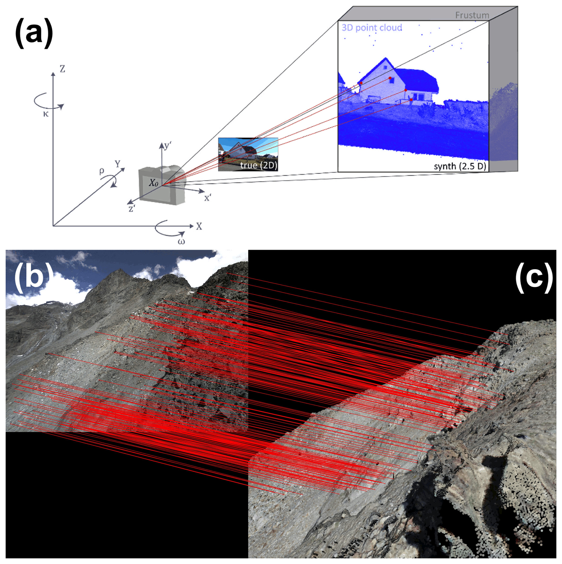
Figure 4 (a) Visualisation of the image-to-geometry scaling (Elias et al., 2023). (b) Real 2D image from Wcam04 being matched (red lines) to (c) the rendered synthetic image derived from the UAV data. Matches focus on the image centre (region of interest), ensuring strong alignment there, while lens distortions remain unmodelled, since no matches are available at the edges, where distortion is expected to be greater.

4.3 Combining PIPs$++$ and GIRAFFE

4.3.1 Image pre-processing

We assumed that the poses of both webcams remained stable over the 19-week observation period. However, we noticed slight movements of Wcam04 caused by wind, which we corrected using a homography-based transformation. Thereby, the first image of the time-lapse sequence is considered the reference to which all subsequent images are registered using SIFT to estimate the points for homography calculation. This calculation is done using the RANdom SAmple Consensus (RANSAC) method to account for potential outliers, such as moving image features in the area of the rock glacier or landslide, which could otherwise introduce errors. The derived homography is then applied to perform a projective transformation of all consecutive images. In this way, the camera model can be considered consistent across all images in the analysed time-lapse sequence; i.e. the images appear as if they were captured from the same perspective. Accordingly, we employed GIRAFFE only to the reference image to ascertain the configuration of the image geometry and utilised the estimated camera model to reference all pixels tracked by PIPs$++$ throughout the sequence in object space.

In contrast to this image-based stabilisation, the camera model of each image of the time-lapse sequence could have been calculated independently of the others via GIRAFFE and then applied to the respective PIPs$++$ image measurements. However, this method was not employed due to the superior robustness of image-based stabilisation, particularly under poor image quality conditions, such as those caused by fog. Note that this type of image pre-processing is only necessary if the camera's geometry appears to change. Otherwise, AI-based feature tracking can proceed directly from the initial images.

4.3.2 Image feature tracking and 3D referencing

We used a NVIDIA RTX A6000 GPU with 48 GB of memory to track 2000 points across a batch size of 19 weekly frames on 3MPx-large images before hitting computational limits. For a temporal window of 19 frames, the same 2000 features were tracked continuously before the grid was reset, after which tracking restarted with the reset grid as new input. Processing 400 images with this setup took approx. 2 min. For validation, specific points of interest, such as boulders with available GNSS/TS data, were tracked in addition to the grid points entered into PIPs$++$. These specific points were inserted into the script as pixel coordinates.

Initial camera specifications for the time-lapse webcams were available from EXIF metadata (i.e. focal length) and GNSS measurements of the camera housings, which were used as approximation for the 3D coordinates of the camera projection centres. For the orientation approximation, it was assumed that the camera was not tiled or rotated along the lateral axes of the reference system. The viewing angle related to the geographic view direction (NESW) was determined by compass. The pitch and roll angles were assumed to be 90° (looking parallel to the XY plane) and 0° (no rotation around the viewing axis). The image points tracked by PIPs$++$ were referenced registering the reference image of the time-lapse sequence to the 3D object space. The camera distortion coefficients could not be determined due to an unsuitable distribution of pseudo-control point observations as large portions of the image were covered by sky and terrain not captured in the 3D UAV data (e.g. Fig. 4).

The resulting lists of 3D coordinates per timestamp, matching the PIPs$++$ feature points, were accompanied by an identifier that allowed the 3D coordinates to be uniquely assigned across the timestamps, enabling the estimation of the per-camera 3D trajectories. Finally, mean velocities in metres per day were calculated dividing the displacement between two consecutive 3D points by the time interval (in this case, 1 week), resulting in a total of 18 weekly velocity measures per tracked image point.

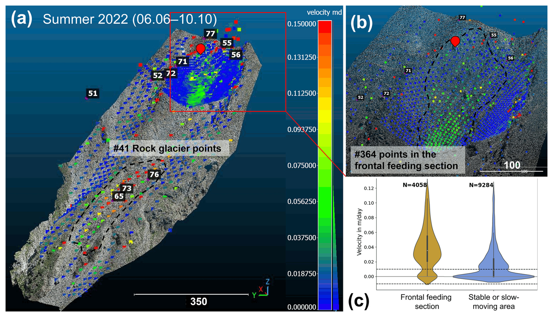
Figure 5 (a) Velocity results (in m d⁻¹) over the entire summer period (127 d) for both the frontal feeding section (upper area, observed by Wcam04) and the rock glacier (lower area, observed by Wcam05), displayed on UAV point cloud data, including total station-measured points (black and white labels) and the permanent GNSS installation (marked with a red location pin). (b) Close-up of the frontal feeding section (Wcam04). (c) Plot of the weekly velocity distribution for both the frontal feeding section and the surrounding stable or slow-moving areas (data from Wcam04), showing a clear noise level between ±0.007 m d⁻¹ in both regions. Dotted lines indicate the moving areas in this study. Points in blue display areas moving less than about 0.02 m d⁻¹ for the considered time frame of 127 d.

5 Results

5.1 Geomorphic results

Our image-based 3D trajectory and velocity measurements were based on two subsets from time-lapse cameras of a permafrost-affected landslide and its frontal section feeding into a rock glacier. The results for both investigated regions of interest for the entire summer period (6 June until 10 October 2022, 19 weekly images) are shown in Fig. 5a. As expected from landform displacements, the results show a largely homogenous flow velocity field with faster velocities on the rock glacier and in the lowermost part of the investigated feeding area from the landslide. The feeding area continues downward and is not captured by either Wcam04 or Wcam05, as evidenced in Fig. 5a. An average movement of 0.03 m d⁻¹ (0.21 m of absolute movement between weekly images) was observed across the entire investigated feeding section, while, in stable and slow-moving areas, movement was typically below 0.01 m d⁻¹ (Fig. 5c). For the rock glacier, the average movement during the summer period was 0.10 m d⁻¹ (0.70 m of absolute movement between weekly images), with surrounding stable or slow-moving areas generally showing displacement rates below 0.05 m d⁻¹ (0.35 m of absolute weekly movement). The feeding section exhibits significant spatial variability: the lowermost part moves fastest (Fig. 5a, b), and, in addition, certain large boulders travel more quickly than their immediate surroundings – unlike the rock glacier, where movement is more uniform.

This revealed variability must be considered when using discrete points from GNSS and TS measurements to characterise landform movement. While the two TS points, used to validate the Wcam05 velocity estimates, show a similar trend to the overall movement of the rock glacier (Fig. 7b), the permanent GNSS reveals a distinctly different movement pattern, with a marked acceleration in velocity at the end of July that is not reflected in the feeding section's overall movement (Fig. 7a).

5.2 Error assessment and validation

The accuracy of the 3D trajectories and velocity derivations essentially depends on three factors: the reliability of the PIPs$++$ feature tracking, the determination of the camera model by image-to-geometry registration, and the resolution and accuracy of the 3D point cloud. To assess the accuracy potential, a comprehensive analysis of all potential sources of error was necessary. However, due to the numerous algorithms, a classic error analysis is difficult, especially because AI-based tools such as PIPs$++$ often do not provide any information on reliability. We have included the following methods in our evaluations:

• Level of detection (LoD). Assessing pseudo-movements in stable areas resulting from an accumulated error of PIPs$++$ measurements and its translation into object space define a so-called LoD, describing the threshold of significant movements that could be detected with our method.

• Theoretical accuracy analysis based on the reprojection results of GIRAFFE.

• Validation with ground truth data by comparing our 3D trajectories based on time-lapse images with GNSS and TS data serving as ground truth at selected 3D objects.

5.2.1 Level of detection

The LoD was experimentally determined analysing the detected 3D movements in presumably stable or slow-moving areas (Fig. 5c). For Wcam04, the designated area lies within the broader zone of the deep-seated landslide (Fig. 1a, blue polygon). While this area moves significantly more slowly than most of the frontal feeding section, its stability is relative and only valid when considered over a short time frame. Here we detected an LoD of about 0.007 m d⁻¹ or an absolute movement of ±5 cm between weekly time-lapse images. For Wcam05, the LoD was around 0.02 m d⁻¹ or an absolute movement of ±14 cm between weekly image frames, which is consistent with the larger camera-to-object distance (Table 1).

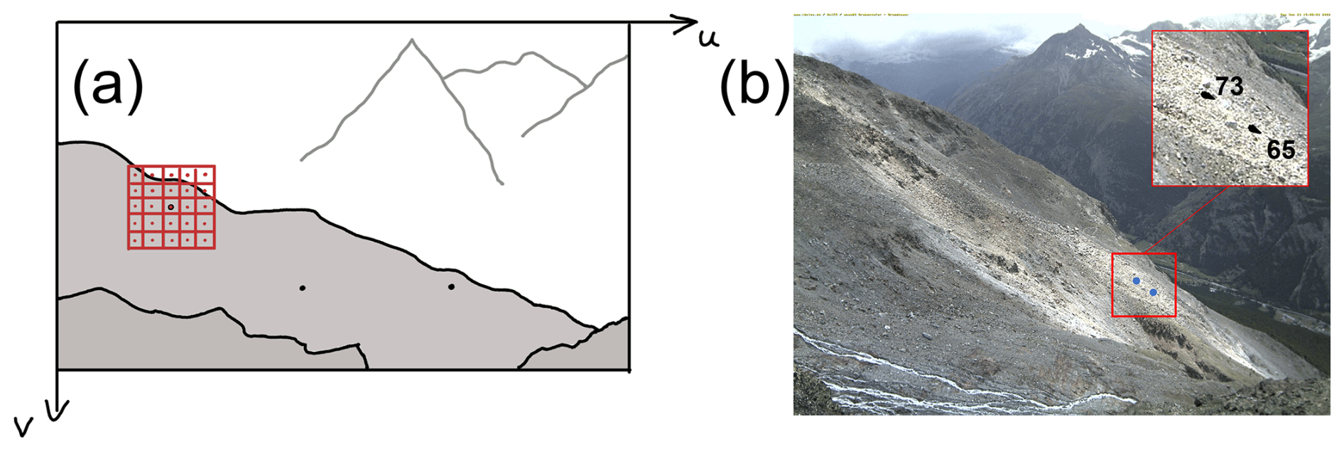
Figure 6 Validation principle illustrated through direct comparison of two measured point trajectories (ground truth) and their corresponding trajectories derived from time-lapse images. Illustration of the tracking principle used for 3D trajectory validation. (a) A 5×5 pixel grid around each ground truth captures local movement. (b) Location of the two validation points on the rock glacier observed by Wcam05.

5.2.2 Theoretical accuracy analysis

For both the stable (Wcam05) and software-stabilised (Wcam04) time-lapse image series, the GIRAFFE software was employed once to estimate the linear camera model of the reference image. To assess the precision of the image-to-geometry registration, GIRAFFE calculates the overall root-mean-square error (RMSE). This is achieved by projecting the 3D pseudo-control points used for space resection back into the image using the estimated camera model and measuring the mean distances between the original image observations and their projected positions. The RMSE for Wcam04 and Wcam05 was 4.8 pixels and 4.5 pixels, respectively.

A theoretical accuracy analysis shows that, for Wcam04, with a camera-to-object distance of 100–350 m and GSDs of 0.06–0.21 m (see Table 2), a 4.8-pixel error leads to positional errors of 0.3–1.0 m. For Wcam05, at 700–1100 m with GSDs of 0.40–0.62 m, a 4.5-pixel error results in 1.8–2.8 m errors. Increased distance amplifies errors from camera geometry uncertainties, leading to higher inaccuracies for Wcam05. GIRAFFE mitigates this with outlier filtering, retaining 3D points with reprojection errors under 2.5 pixels, corresponding to object space errors of 0.10–0.40 m for Wcam04 and 1.0–1.2 m for Wcam05.

5.2.3 Validation with ground truth data

To validate our method, we used GNSS and TS ground truth data for selected 3D objects visible in the camera's field of view. Objects with movement below the LoD were excluded. Due to logistical and safety constraints, the ground truth data does not cover the fast-moving areas of the frontal feeding section. However, ground truth data is available in the upper landslide area (Fig. 5b).

For Wcam05, two moving objects on the rock glacier were suitable for direct validation, while, for Wcam04, a permanently installed GNSS antenna provided a reference. Other potential objects were either outside the camera's field of view or had movements below the LoD. Given the challenge of precisely identifying the measured ground truth point in the image data, we tracked 5×5 patches, i.e. 25 pixels, around the presumably image position of the respective object (Fig. 6a).

For the two objects in Wcam05, 3D trajectories were reconstructed across five monthly timestamps, yielding eight validation measurements. To improve robustness against noise and outliers, we validated against fitted 3D trajectory lines using the detected positions in the five timestamps rather than the individual 3D point coordinates. This approach assumes linear motion, which was supported by TS reference data.

We quantified alignment quality by calculating the standard deviation of perpendicular distances between measured points and the fitted trajectory lines. The PIPs$++$/GIRAFFE measurements for Wcam05 (Fig. 6b) showed greater noise than the TS reference data (Fig. 7). However, spatial differences and Euclidean distances between vectors indicated only minor discrepancies, within a few decimetres. This suggests that fluctuations in measured 3D trajectories are random rather than systematic errors. Directional differences between reference and measured trajectories varied by only a few degrees (Table 2). These discrepancies are likely due to imaging geometry challenges (linked to camera configuration detailed in Table 1) and occlusion effects caused by the camera perspective, particularly in the presence of boulders. For Wcam04, the minimal movement of tracked points limited trajectory fitting. Instead, accuracy was estimated using the centre of gravity of the respective 3D point sets. A 1.3 m offset was observed for Wcam04 (Table 2), which is consistent with the GNSS antenna's 1.5–2 m elevation above the surface and its position on the opposite side of the boulder. Because the boulder is roughly the size of a small truck, we performed validation on the opposite side rather than at the true antenna location. Despite this, velocity patterns in GNSS and PIPs$++$/GIRAFFE data remained consistent (Fig. 8a).

Table 2 Calculation of fitted 3D trajectories of significant objects tracked over 109 d with GNSS (one point, visible in Wcam04) and over 118 d with TS (two points, visible in Wcam05) and with PIPs$++$ and GIRAFFE in the associated images, taken on the same days as the GNSS/TS ground truth measurements. SD: standard deviation. Diff: difference.

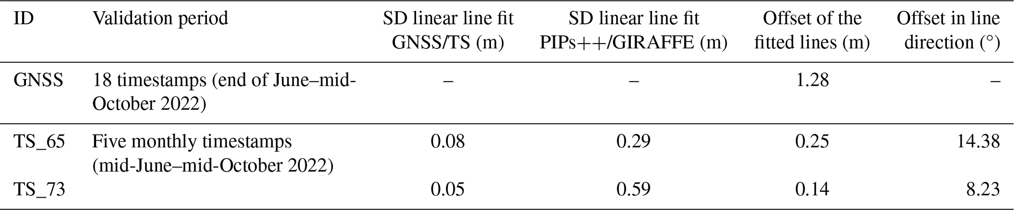
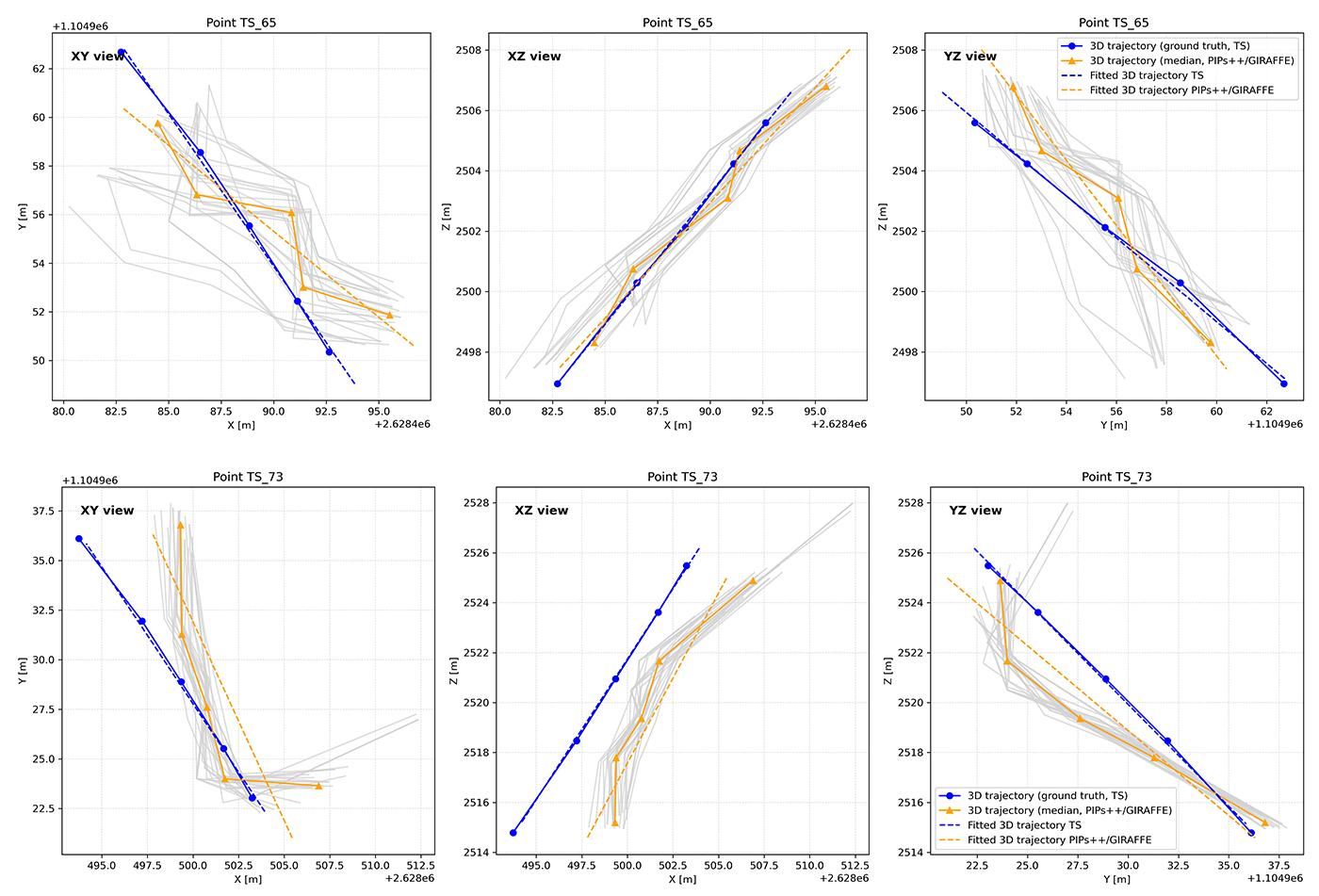
Figure 7 Comparison of 3D trajectory estimations from theodolite measurements (TS) and tracking data (PIPs$++$/GIRAFFE) across different 2D projections for two points (named 65 and 73). The XY, XZ, and YZ views show individual point trajectories with their respectively fitted 3D lines. Light-grey lines represent all time-lapse trajectories, while blue and orange markers correspond to the theodolite and median of the tracking data, respectively. Dashed lines indicate the best-fit linear 3D trajectory for each method.

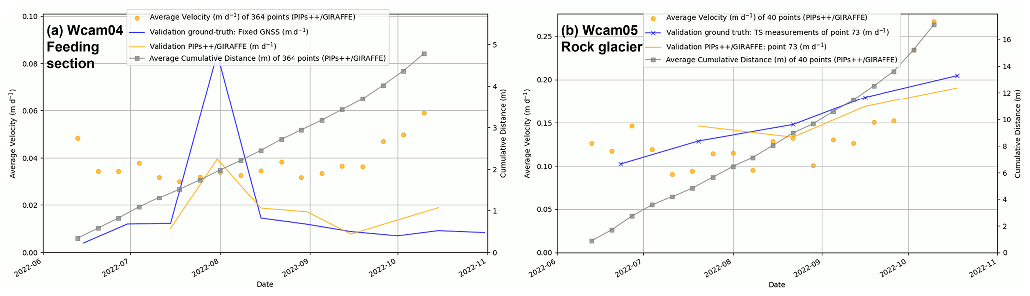
Figure 8 Graphs showing weekly velocities and cumulative distances of tracked points measured using the PIPs$++$/GIRAFFE workflow, including validation against ground truth data. (a) Feeding section (Wcam04) and (b) rock glacier (Wcam05) during summer 2022, derived from time-lapse imagery. Note that the data from 26 October are excluded from panel (a) due to foggy conditions and were interpolated by the model. Validation points, marked with a solid blue line, represent measurements from a permanent GNSS antenna installed on a large boulder in the upper feeding area (a) and one theodolite point on the rock glacier (b). The corresponding tracked points by PIPs$++$/GIRAFFE are displayed with a solid orange line.

6 Discussion and limitations

6.1 General performance of the proposed workflow

The methodology described above has the potential to tackle entire time-lapse image datasets to determine landform velocities, in this case creeping permafrost landforms. The results of our workflow show a good agreement with GNSS and TS theodolite measurements considering the low-grade cameras used (Table 2, Fig. 7), proving our method to be reliable, robust, and fast for creating a better spatial (Fig. 5) and temporal (Fig. 8) coverage of the landform's displacement. Our pilot study demonstrates that significant motion and velocity information can be rapidly extracted using AI-based methods from a basic, cost-effective device such as a single webcam, greatly enhancing temporal acquisition frequency without the need for a camera array. Spatial heterogeneity of landform movement is evident as well, including instances where larger boulders move faster, seemingly “surfing” on the main landslide body. This phenomenon, illustrated in Fig. 8a, is supported by in situ GNSS data, which indicate faster movement compared to the overall landform. If this pattern were seen across the entire landform, it could suggest motion linked to permafrost creep or specific movement in the active layer, often triggered by significant water input from snowmelt or rainfall (RGIK, 2023). However, the movement is mostly restricted to large boulders, possibly pointing to a gravitational origin due to the steep terrain. The uppermost landslide area and the lower rock glacier are presumably driven primarily by permafrost creep. However, the driving mechanisms of the frontal feeding section observed by Wcam04 remain unknown. To better understand the factors controlling velocity changes and the overall behaviour of these landforms, further investigation into environmental drivers such as rainfall and temperature is necessary – especially considering the exceptionally warm and dry summer of 2022, which featured consecutive heat waves. Our developed method provides a framework for such future research, enabling the analysis needed to address these open questions.

Although our proof of concept did not achieve the millimetre to centimetre accuracy of GNSS and TS measurements, we were still able to detect absolute displacements of 5 and 14 cm between consecutive frames (in our case weekly) using the setups of Wcam04 and Wcam05, respectively (Table 1). The measurements at the rock glacier (Wcam05) have a significantly lower spatial resolution (41 vs. 364 points tracked in the feeding area) due to the greater distance of the webcam from the area of interest and its suboptimal viewing angle (Fig. 1b). The increased distance also made the measurements more sensitive to slight camera movements, which, along with the lower LoD, likely contributed to some of the higher variation in computed rock glacier velocity (Fig. 7b). The output of our workflow yields a sparse point cloud for every image frame in the sequence with absolute distance and velocity information as a scalar field, as visualised in Fig. 5. This provides a great amount of spatial and temporal data in a manageable file format suitable for big data.

The superior performance of the PIPs$++$ model stems from tracking multiple time steps jointly instead of frame by frame, enhancing temporal smoothness and coherency and improving flow estimation accuracy (Hur and Roth, 2020). This makes PIPs$++$ especially suitable for environmental applications, where, for example, changes in light conditions are a common problem. Moreover, PIPs$++$ is trained on a very large and diverse artificial dataset, PointOdyssey (Zheng et al., 2023), including rendered dynamic fog to account for (partial) occlusion and realistic in- and outdoor scenes. This is entirely absent from other synthetic datasets such as the FlyingChairs dataset, which was utilised to train models such as FlowFormer (Huang et al., 2022) or GMFlow (Xu et al., 2022), i.e. transformer-based models, and justifies our use of PIPs$++$ as a tracker in this proof of concept without the need to re-train the model with a sample of our own data. While previous research, using monoscopic images to track a landslide (Travelletti et al., 2012) and a rock glacier (Kenner et al., 2018), was prone to mismatches because of its frame-by-frame strategy, our approach surpasses this limitation and at the same time makes it possible to process longer time periods and handle big data collected by hourly webcams more adequately. By tracking points in stable areas using either hand-crafted point operators such as SIFT or AI-based methods, shifts in camera position, a common problem in long time-lapse imagery sequences, can be corrected to some degree to stabilise the image sequence by software. When using PIPs$++$ and GIRAFFE, two options exist to deal with camera movements: (a) image stabilisation by software or (b) individual referencing of each time-lapse image, i.e. running GIRAFFE image per image. The correction based on image pixels is frequently accomplished through the calculation of a homography to match a reference image. However, because the method assumes a planar scene, it can only partially compensate for perspective distortions caused by camera movements. Consequently, it is suitable for smaller movements. In cases of stronger movements, we recommend calculating the camera model for each individual image of the image sequence. As a result, even major changes in perspective should be handled adequately when translating the image measurement into object space.

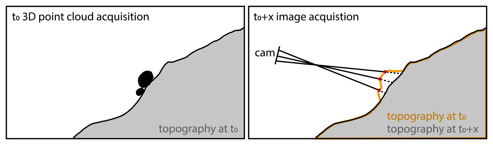
Figure 9 Illustration of the georeferencing validity issue when using a 3D point cloud acquired at time t₀ to transfer image measurements from a time-lapse image captured after significant topographic changes. In this example, boulders present during the initial 3D data acquisition have since disappeared. Consequently, image rays intersect the outdated modelled topography, resulting in erroneous coordinates. These errors propagate into derived 3D trajectories and velocities. The greater the topographic changes between the reference data and affected image measure, the larger the error. Therefore, the reference topography should ideally reflect the conditions at the time of image acquisition.

6.2 Limitations

As PIPs$++$ still relies on appearance-matching cues similar to traditional methods, it remains sensitive to abrupt changes in appearance, such as substantial variations in snow cover or alterations in surface morphology due to e.g. extensive rockfalls. This issue was also highlighted as a major limitation by Kenner et al. (2018). However, because the algorithm can quickly process large amounts of data, we can leverage the full temporal resolution, allowing tracking to succeed as long as snow cover changes gradually, as shown in Fig. 3d.

Another important limitation of our approach is that PIPs$++$ does not perform well in detecting movements for every pixel in the image due to the use of a regular grid compared to other frame-to-frame approaches. Currently, a regular grid size of 2000 points per image is used, limited by computational power. While PIPs$++$ works well with the low-resolution images in this study, higher-resolution images quickly reach the limits of our available computational resources. One major limitation is the need for specific and expensive computational setups (e.g. a NVIDIA RTX A6000 GPU with 48 GB). Even with these resources, increasing the temporal window, image resolution, and tracked points can quickly hit the limits. Considering appropriate GPU and CPU computational power, around 15 min was needed to process the example dataset of this paper in an end-to-end fashion, from raw time-lapse images to velocity graphs. The majority of this time is needed to scale the output of the PIPs$++$ model with GIRAFFE, which is highly dependent on the size of the 3D point cloud.

Ideally, the 3D point cloud used in GIRAFFE for image-to-geometry registration reflects the imaging situation at the time of the time-lapse image measurements, thereby avoiding intersection errors resulting from significant changes in surface topography (Fig. 9). Despite the temporal gap of approximately 1 year between the time-lapse image subsets and the 3D data, we assume that the overall topography has remained largely unchanged. Moreover, significant errors arising from potential discrepancies between the image content and the 3D surface are expected to be rejected in the outlier analyses in GIRAFFE. Such mismatches are unlikely to align with the estimated camera model, as the model calculation relies on pseudo-control points that are more evenly distributed and exhibit strong agreement between the image content and the object surface. Nevertheless, minor inaccuracies caused by isolated structural changes (e.g. displacement of boulders) cannot be entirely ruled out. Such discrepancies can only be identified when analysing the movement trajectories as a whole. Furthermore, the quality of the image-based 3D trajectories is heavily correlated to the quality of the point cloud data.

Additionally, a suboptimal oblique viewing angle, such as with Wcam05 (Fig. 1b), can complicate the matching process, as the rendered view will be limited to a narrow strip. This can affect the distribution of matches and compromise the estimation of the camera's interior orientation and lens distortions (Elias et al., 2019).

There is still potential to optimise the proposed workflow to achieve full automation for processing entire image sequences. This includes automatically detecting moving and stable areas, which currently relies on user-defined criteria and thus depends on prior site knowledge. Additionally, we need to conduct further investigations into the in-field calibration of intrinsic camera parameters, especially the image distortion, and their stability over time (Elias et al., 2020). Improvements in 2D-to-3D tools (like GIRAFFE) also benefit other disciplines, such as the quantitative analysis of historical terrestrial photographs for mapping historical rockfalls (Wegner et al., 2023) and changes in glacier forefields (Altmann et al., 2020).

The developed workflow could prove valuable for analysing monoscopic time-lapse image sequences of other dynamic processes, such as lava flows (James and Robson, 2014), solifluction and gelifluction movements (Matsuoka, 2014), and flow velocities in rivers (Eltner et al., 2020; Stumpf et al., 2016). Given the prevalence of time-lapse camera data collection, a rapid and efficient method for automatically processing such extensive datasets holds significant scientific relevance. Furthermore, the fast and robust processing of the time-lapse imagery makes it possible to function as an early warning system when processing can be carried out in near real-time, as indicated by Kenner et al. (2018).

7 Conclusions

This proof of concept demonstrates the potential of AI-based algorithms for tracking and matching points to improve motion estimations in time-lapse image sequences of a mountain landscape. Two fast-moving alpine landforms – a landslide and a rock glacier at the Grabengufer site in Switzerland – were selected as the pilot study area. The initial results presented in this paper show that robust and reliable velocity information can be quickly derived with minimal input data and user intervention. Our pilot study opens the door to processing entire image datasets to reveal spatiotemporal patterns that traditional monitoring methods have previously overlooked, due to their limited spatial or temporal resolution and the inadequate computational and algorithmic power to handle large image datasets.

The PIPs$++$ model, used for tracking features in image sequences, excels in widening the temporal window and includes a template update mechanism that allows changes in feature appearance. Its key advantage is its ability to accurately estimate occluded trajectories within the temporal frame, avoiding suboptimal matches and enhancing tracking accuracy, making it especially robust for environmental applications and eliminating the need for filtering blurry or foggy images as a pre-processing step. Additionally, the model's rapid performance, processing 400 images in 2 min to track features through a temporal window of 19 frames, is promising for handling large datasets and developing early warning systems. The image-to-geometry approach, implemented in GIRAFFE, provides an accurate way to scale the 2D image data into 3D object space, even under suboptimal camera viewing angles and distance to the area of interest.

This paper represents an important step forward in using monoscopic cameras and leveraging previously captured data that have not been processed automatically with metric values before. By significantly enhancing temporal acquisition frequency using basic time-lapse imagery, we can achieve a level of data resolution that would be expensive with in situ differential GNSS and georeferenced TS measurements or UAV and TLS or ALS methods. Our approach provides a spatially continuous understanding of landform movement. It allows data acquisition in areas where in situ measurements are impractical due to logistical and safety constraints and where other remote sensing techniques fail due to high landform displacements. Furthermore, depending on the image resolution, distance to the landform, and its velocity, our approach can achieve a sub-seasonal resolution of velocity information with an accuracy of several centimetres. This study introduces a new open-source tool for scientists to automatically extract metric information from existing webcam datasets, extending its applicability to further environmental process observations.