Grain size dynamics using a new planform model – Part 1: GravelScape description and validation

The grain size preserved within the stratigraphic record over thousands to millions of years has several important applications. In particular, it can serve as a record of significant climatic, eustatic, or tectonic events. Here we present a new model for grain size fining predictions that combines a landscape evolution model based on the Stream Power Law but modified for sedimentation (Yuan et al., 2019) with an extension of the self-similar grain size model (Fedele and Paola, 2007). The new model, which we called GravelScape, includes the effects on grain size fining of lateral heterogeneities in deposition rate caused by dynamically evolving channels. We show that, when multi-channel dynamics (i.e. avulsions) are prevented, by reducing the planform model to a single downstream dimension, our new model can reproduce results obtained by other methods that assume that fining is controlled by subsidence only. We demonstrate that including across-basin (two-dimensional) effects can lead to deviations from previous subsidence predictions for grain size fining. The magnitude of these deviations correlates with the extent of sediment bypass and the configuration of surface topography, both of which influence the amplitude of across-basin variability within the sedimentary system.

1 Introduction

Grain size trends in the stratigraphic record are widely used as an important source of information about past and present depositional environments. As postulated by Allen et al. (2013) and Duller et al. (2010), the ratio of sediment flux to accommodation not only controls basin filling, deposition, and fan development but also strongly influences downstream fining for gravel and sand coarse fractions. When used within their geologic context, variations in grain sizes can be used to identify changes in past environmental conditions that have been recorded in the stratigraphic record (Armitage et al., 2011; Rice, 1999). For example, increasing precipitation within the source catchment results in a lateral shift in where coarser grains are deposited and a lengthening of the fan area in response to the accompanying increase in sediment flux (Armitage et al., 2011). Hooke (1968) suggests that higher tectonic uplift and tilting within the Panamint Range produce higher sediment flux in the western part of Death Valley, leading to more extensive coarse-grained alluvial fans relative to the eastern Black Mountains area. As postulated by Duller et al. (2010) and observed by Dingle et al. (2016) within the Ganga Plain, grain size fining rate is more rapid in short, rapidly subsiding systems. Multiple further examples (i.e. Harries et al., 2018; Paola et al., 1992; Whittaker et al., 2011; Brooke et al., 2018) highlight how a thorough understanding of grain size fining in response to external forcing has broad implications for interpreting the sedimentary record to unravel tectonic conditions and climates of the geological past.

There are a number of internal dynamical processes that are also likely to impact the coarse grain size record depending on sediment flux, discharge, subsidence rate (or the creation of accommodation space), and basin geometries (Sømme et al., 2009; Scheingross et al., 2020; Romans et al., 2016; Hajek and Straub, 2017). These internal or autogenic processes, such as basin reorganization, sediment waves, channel avulsions, or knickpoint generation (Scheingross et al., 2020), arise due to strong feedbacks between topography, erosion, and sediment transport that are independent of external perturbations. Their impact on grain size fining has been, however, largely excluded from previous theoretical and modelling studies that predict grain size fining.

Modelling studies (Veldkamp et al., 2017; Carretier et al., 2016; Armitage et al., 2011; Davy and Lague, 2009; Paola and Voller, 2005) commonly predict how external forcings control the grain size in the stratigraphic record, based on reduced-complexity approaches. This is because hydraulic processes controlling grain size as observed in modern systems are often too complex to model over millions of years, and their characteristics are, for the most part, not preserved within the geologic record. For example, Fedele and Paola (2007) have developed a reduced-complexity model of depositionally controlled grain size fining using concepts derived from the stratigraphic record, such as time-integrated grain size self-similarity. The self-similar grain size fining model assumes that downstream deposition is the main control on the fining rate (Fedele and Paola, 2007) and, thus, does not consider feedbacks between grain size and topography.

Many past grain size modelling approaches for the stratigraphic record (Veldkamp et al., 2017; Carretier et al., 2016; Armitage et al., 2011; Davy and Lague, 2009; Paola and Voller, 2005) have in common that they consider fining along a single main channel transporting sediment from source to sink. Consequently, they do not address the complexity of most natural sedimentary systems, where transport and deposition occur along several channels that are characterized by a very dynamic behaviour that is likely to influence grain size fining and the way it is stored in the stratigraphic record.

This is the main motivation for the new method that we developed and present here that generalizes the self-similar gravel grain size model of Fedele and Paola (2007) into multiple dimensions (downstream, across the basin, and overtime/depth) using a planform landscape evolution model, FastScape (Braun and Willett, 2013), that allows for erosion and deposition (Yuan et al., 2019) following the approach developed by Davy and Lague (2009). Because the model can represent deposition and erosion in two dimensions, i.e. along several dynamic channels, it can update topography at each time step, and because it does not rely on the common assumption that deposition rate must be equal to subsidence rate (Duller et al., 2010; Whittaker et al., 2011), it should allow us to investigate the impact of external forcings and internal processes on grain size fining and therefore help us to better understand the sedimentary record.

In this paper, we first provide a short description of the model by Fedele and Paola (2007) for self-similar grain size fining and of the landscape evolution model (FastScape) that we have used. We then describe how we have combined the two to propose a new, planform model for self-similar grain size fining, which we called GravelScape (see supplement video for an example of the model). We describe its basic behaviour and compare its results to the sediment fining curves obtained by Duller et al. (2010) along a single channel, assuming an exponential shaped subsidence function simulating a flexural basin and a constant sediment flux at steady state into the basin. We will use these results to validate our numerical approach but also to demonstrate that differences are likely to be driven by autogenic processes that can only be modelled with a two-dimensional, planform approach.

This paper is the first of a series of three that report our recent work on modelling grain size fining in two-dimensional sedimentary systems. As explained above, the first focuses on the description of the multi-channel, Landscape Evolution Model (LEM)-coupled grain size model, its general behaviour at steady state, and its validation by comparison with single-channel work by Duller et al. (2010). The second paper (Wild et al., 2025b) will be devoted to studying autogenic processes and how they affect preserved grain size under many different basin setups at steady state. The third paper (Wild et al., 2025c) expands beyond the steady-state hypothesis to focus on foreland basin evolution and how autogenic dynamics and the resulting grain size fining are likely to behave and are stored in the stratigraphic record at various phases of basin evolution.

2 Previous work on which our model is based

2.1 The self-similar grain size model of Fedele and Paola (2007)

The underlying approach for our integration of grain size fining into a landscape evolution model is based on grain size solution (D) by Fedele and Paola (2007) as a function of dimensionless distance downstream (x^*) within a depositional area for gravel,

$$\begin{array}{}\text{(1)}& D\left(x^{*}\right)=\stackrel{\mathrm{‾}}{D_{\mathrm{0}}}+{\mathit{\varphi }}_{\mathrm{0}}{\displaystyle \frac{C_{\mathrm{2}}}{C_{\mathrm{1}}}}{e}^{-C_{\mathrm{1}}{y}^{*}}-\mathrm{1},\end{array}$$

and sand,

$$\begin{array}{}\text{(2)}& D\left(x^{*}\right)=\stackrel{\mathrm{‾}}{D_{\mathrm{0}}}{e}^{-C_{\mathrm{3}}{y}^{*}},\end{array}$$

where x^* is the distance along the river profile, x, normalized by its total length ($x^{*}=x/L$). $\stackrel{\mathrm{‾}}{D_{\mathrm{0}}}$ and ϕ₀ are the initial mean grain size and standard deviation at the source, respectively. C₁,C₂, and C₃ are constants that represent the change in mean grain size and standard deviation downstream. C_v is defined as the ratio of the downstream change in the standard deviation relative to mean grain size, i.e. $C_v=C_{\mathrm{1}}/C_{\mathrm{2}}$, and referred to as the coefficient of variation. C₁ ranges between 0.5 and 0.9, C₃ between 0.1 and 0.45, and C_v between 0.7 and 0.9 (Fedele and Paola, 2007). Whittaker et al. (2011) note that a C_v value of 0.8 is commonly observed. Note that, to avoid repetition, this work will focus on the application of the gravel equation (Eq. 1), but all methods described further below could be modified and applied to solving the sand equation (Eq. 2).

As defined in Fedele and Paola (2007), y^* is the dimensionless distance transformation given by

$$\begin{array}{}\text{(3)}& y^{*}\left(x^{*}\right)=\underset{\mathrm{0}}{\overset{x^{*}}{\int }}{R}^{*}\left(x^{*}\right)\mathrm{d}{x}^{*},\end{array}$$

where R^* is the dimensionless downstream distribution of deposition defined as

$$\begin{array}{}\text{(4)}& R^{*}=(\mathrm{1}-\mathit{\gamma })RL,\end{array}$$

where γ is the porosity of the sediment deposit, and R is the ratio of deposition rate, r, to sediment flux, q_s, i.e. $R=r/q_{\mathrm{s}}$. At each x^* point along the river profile, R^* relates the sediment deposition into the substrate to the sediment flux in the river, taking into account a given length and porosity. Finally, deposition rate, r, is the sum of the rate of change of elevation of the landscape and the subsidence rate, σ, i.e. $r=\mathrm{d}h/\mathrm{d}t+\mathit{\sigma }$.

In non-mathematical terms, the approach of Fedele and Paola (2007) postulates that grain size fining over long timescales is controlled by (1) the source sediment supply and grain size distribution; (2) the deposition rate throughout the system length; (3) the hydraulic mobility of different grain size types (gravel vs. sand) assuming a constant shield stress at the bed; (4) self-similarity between the subsurface and surface of the distribution of gravel grain size clasts; and (5) a mass balance of the transport, substrate, and an active layer (Fedele and Paola, 2007). We refer the reader to Fedele and Paola (2007) for a more detailed explanation of the assumptions behind this model and how it has been derived from these assumptions. However, the self-similarity of gravel grain sizes has now been repeatedly demonstrated from field data (D'Arcy et al., 2017; Harries et al., 2018; Brooke et al., 2018), and this model has been successfully applied to stratigraphic examples (Whittaker et al., 2011; Duller et al., 2010; Garefalakis et al., 2024).

2.2 The Landscape Evolution Model (LEM)

We use FastScape (Bovy et al., 2023; Bovy and Lange, 2023) as a basic Landscape Evolution Model (LEM) that solves the Stream Power Law (SPL) in two dimensions following the efficient algorithm described in Braun and Willett (2013). The SPL states that the rate of bedrock elevation change is the sum of uplift (or subsidence) rate U and erosion rate assumed proportional to upstream drainage area, A, used as a proxy for discharge, and local slope S (Whipple and Tucker, 1999):

$$\begin{array}{}\text{(5)}& {\displaystyle \frac{\mathrm{d}h}{\mathrm{d}t}}=U-K{A}^m{S}^n,\end{array}$$

where K is a rate coefficient or erosivity that depends mostly upon lithology and precipitation rate. m and n are exponents that generally maintain a ratio of $m/n\approx \mathrm{0.5}$. Sediment transport and deposition are incorporated into FastScape using the implementation of Yuan et al. (2019) of the ξ−q's algorithm by Davy and Lague (2009), which states that the rate of sediment deposition is proportional to sediment flux and inversely proportional to upstream drainage area. This leads to the following evolution equation that integrates the processes of uplift/subsidence, erosion, transport, and deposition into a simple framework:

$$\begin{array}{}\text{(6)}& {\displaystyle \frac{\mathrm{d}h}{\mathrm{d}t}}=U-K{\stackrel{\mathrm{̃}}{p}}^m{A}^m{\left({\displaystyle \frac{\mathrm{d}h}{\mathrm{d}s}}\right)}^n+{\displaystyle \frac{G}{\stackrel{\mathrm{̃}}{p}A}}\underset{A}{\int }\left(U-{\displaystyle \frac{\mathrm{d}h}{\mathrm{d}t}}\right)\mathrm{d}A.\end{array}$$

In this formulation, G is a dimensionless deposition coefficient, and $\stackrel{\mathrm{̃}}{p}$ represents spatial or temporal variations in precipitation rate with respect to a mean value that is contained in both K and G. In this work, we will vary topography through G and discuss its impact on model results. G controls the transport- or detachment-limited nature of the depositional system (Yuan et al., 2019). Guerit et al. (2019) have demonstrated that many natural river systems tend to be on the transport limited side. Note that, for numerical reasons, G=1 is the maximum transported-limited value computed efficiently and reliably by FastScape (Yuan et al., 2019), although larger values can be used but may require multiple iterations and reduce efficiency. Reducing G reduces the transport limited nature of the system and moves into more of a detachment limited setup.

In FastScape, in order to compute the transport of water and sediment, nodes are ordered along flow paths through the landscape. This is performed by creating a stack order using single- or multiple-receiver algorithm. Both algorithms allow for the formation of multiple channels, but the single-receiver algorithm is limited to flow convergence, while the multiple-receiver algorithm permits flow divergence. Both are therefore different from the single-channel approach that is common to all previous applications of the self-similar grain size fining model. In all the model results presented here, we have used the multiple-receiver algorithm, in which the proportion of water and sediment that is given from one node to its downslopes' neighbouring nodes is proportional to slope.

In FastScape, uplift and subsidence rate are imposed as functions of space and time, but they can also be obtained by solving the flexure equation representing flexural isostasy of the lithosphere/crust system.

3 A model for grain size fining including lateral heterogeneity: GravelScape

3.1 Coupling: incorporating the self-similar grain size model into FastScape

We have generalized self-similar approach of Fedele and Paola (2007) to two dimensions, i.e. following flow path, s, or the stack node ordering computed in FastScape. We call our algorithm GravelScape. For this, we replace any spatial integration or differentiation along the normalized river distance by its equivalent value along the normalized steepest descent flow path, $s^{*}=s/L_s$, where L_s is the total length of the flow path. For example, the deposition rate is the spatial derivative of the flux along that flow path:

$$\begin{array}{}\text{(7)}& {\displaystyle \frac{\partial q_{\mathrm{s}}}{\partial s}}={\displaystyle \frac{\mathrm{1}}{L_s}}{\displaystyle \frac{\partial q_{\mathrm{s}}}{\partial s^{*}}}.\end{array}$$

In practice, we first compute the flow path and erosion/deposition rate along the flow path using the multiple-receiver routing in FastScape. Next, sediment flux is computed by summing the erosion/deposition rate, r, down the flow path. Note that, where deposition takes place, r is negative and consequently decreases the sediment flux q_s in the summation along the flow path to the limit of q_s=0. Once q_s is computed, the downstream distribution of deposition R can be calculated according to

$$\begin{array}{}\text{(8)}& R=\left\{\begin{array}{ll}(\mathrm{1}-\mathit{\gamma })\frac{r}{q_{\mathrm{s}}}& \mathrm{if}r,q_{\mathrm{s}}>\mathrm{0}\\ \mathrm{0}& \mathrm{otherwise}\end{array}\right..\end{array}$$

Next, the dimensionless distance transformation y^* is computed from a weighted summation of R through the nodal stack. Where flow converges, a weighted mean is used to compute the receiver y^* values, where the weights are proportional to the upstream drainage area size of the donor nodes. In this way, when multiple flow paths converge, the largest drainage area flow path will dominate the downstream grain size distribution. Such an approach matches observations that grain size distributions of larger catchment rivers tend to dominate downstream grain size distributions (Harries et al., 2019).

Finally, using y^*, we compute the mean grain size using Eqs. (1) or (2). In these equations, the value for D₀ is needed at every grid point within the model. For this, we compute a field D₀ that is obtained by propagating the value of the grain size last deposited on the bed (which we call D_t) down the flow path of a given time step from where the channel originates. Using D₀ defined in this way at each grid point, we use Eq. (1) or (2) to calculate a grain size value, D_x, at all points of the grid where deposition occurs, which we also use to update D_t for the following time step. At the start of the simulation, D₀ and D_t are set equal to the mean grain size as produced by bedrock erosion in the mountain catchment. Note that deposition does not take place at every grid point at every time step, so D_t is only updated to the newly computed grain size D_x where net deposition takes place. Finally, local erosion may take place in the basin, causing an increase in sediment flux and a reduction in D_x fining rates.

In summary, we carry three grain size values at every grid point: (1) the grain size of material deposited at the current time step (D_x); (2) the grain size at the surface of the model, i.e. of the material last deposited at that point (D_t); and (3) the grain size in the “source” area, i.e. where the flow path traversing the grid point originated (D₀). We show in Fig. S1 in the Supplement. computed values of D₀, D_t, and D_x for a given time step under the assumption of single and multiple-receiver routing. In the work presented here, we will only show computed grain size values using the multiple-receiver algorithm.

3.2 Model setup

To illustrate the behaviour of the new model and, most importantly, to compare it to previous studies which computed grain size fining along a single, main channel, we chose a setup that is similar to that used by Duller et al. (2010). As shown in Fig. 1, this setup is composed of two regions, one subjected to uplift (the source or mountain region of length L_M) and the other to subsidence (the basin region of length L_B). Although our model is two-dimensional, the uplift and subsidence are assumed to be functions of one of the two horizontal components only, i.e. the x coordinate. Following the setup of Duller et al. (2010), the subsidence, σ(x), in the basin area is given by

$$\begin{array}{}\text{(9)}& \mathit{\sigma }\left(x\right)={\mathit{\sigma }}_{\mathrm{0}}{e}^{-\mathit{\alpha }x/L_{\mathrm{M}}},\end{array}$$

where σ₀ is the subsidence at the orogenic front (i.e. at the limit between the source and basin areas, where x=0), and α is the rate of decay of the subsidence away from the front. Large values of α result in most of the subsidence near the source, while small values of α result in a more distributed subsidence across the basin. This exponential function mimics subsidence curves resulting from flexure of the underlying lithosphere/crust under the weight of the topography created by uplift in the source area relatively well, without any lateral heterogeneity.

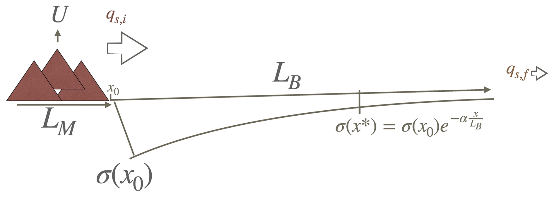
Figure 1 Sample basin setup using Duller et al. (2010) imposed subsidence. All figures within this work will be draining an orogenic front to the left to an eventual sink to the right, even if only results within the basin are shown.

Duller et al. (2010) do not explicitly model the source area but assume a constant sediment flux, q_s,i, originating from it. To reproduce this setup, we will assume that the source area uplifts at a rate U chosen such that $q_{s,i}=(\mathrm{1}-\mathit{\gamma })U{L}_{\mathrm{M}}$. In our setup, we will need to run the model for a sufficiently long period of time for it to reach steady state so that the flux is constant, and our results become comparable to those of Duller et al. (2010). Note that the values of the various LEM parameters, i.e. K, m, n, and G, do not influence the value of the steady-state flux coming out of the source area, only the time it will take to reach the steady state.

We can then follow Duller et al. (2010) and introduce a quantity, F (see Fig. 2), that is the ratio of the flux coming out of the source, q_s,i, to the flux of sediment that is trapped in the basin. As demonstrated by Duller et al. (2010), F and α are the major controls on the relative rate of grain size fining across the basin. F can be written as

$$\begin{array}{}\text{(10)}& F=q_{s,i}/\underset{\mathrm{0}}{\overset{L_{\mathrm{B}}}{\int }}\mathit{\sigma }\left(x\right)\mathrm{d}x,\end{array}$$

where F indicates the under-filled, over-filled, or filled state of the basin. When F is larger than 1 there is more incoming flux, q_s,i, than the basin subsidence can accommodate, producing an outflow of sediment from the basin ($q_{s,f}>\mathrm{0}$). In contrast, when F is smaller than 1, the basin is under-filled, and no sediment leaves the basin ($q_{s,f}=\mathrm{0}$). Here, systems that are characterized by F values lower than or equal to 1 will be referred to as under-filled or limited-bypass systems. Systems where F is greater than 1 but less than or equal to 10 will be referred to as filled or low-bypass systems (Fig. 2a). Systems where F is greater than 10 will be referred to as over-filled or high-bypass systems (Fig. 2b). In Fig. 2c we show how varying σ₀ while keeping both α and $q_{s_i}$ constant leads to different values for F.

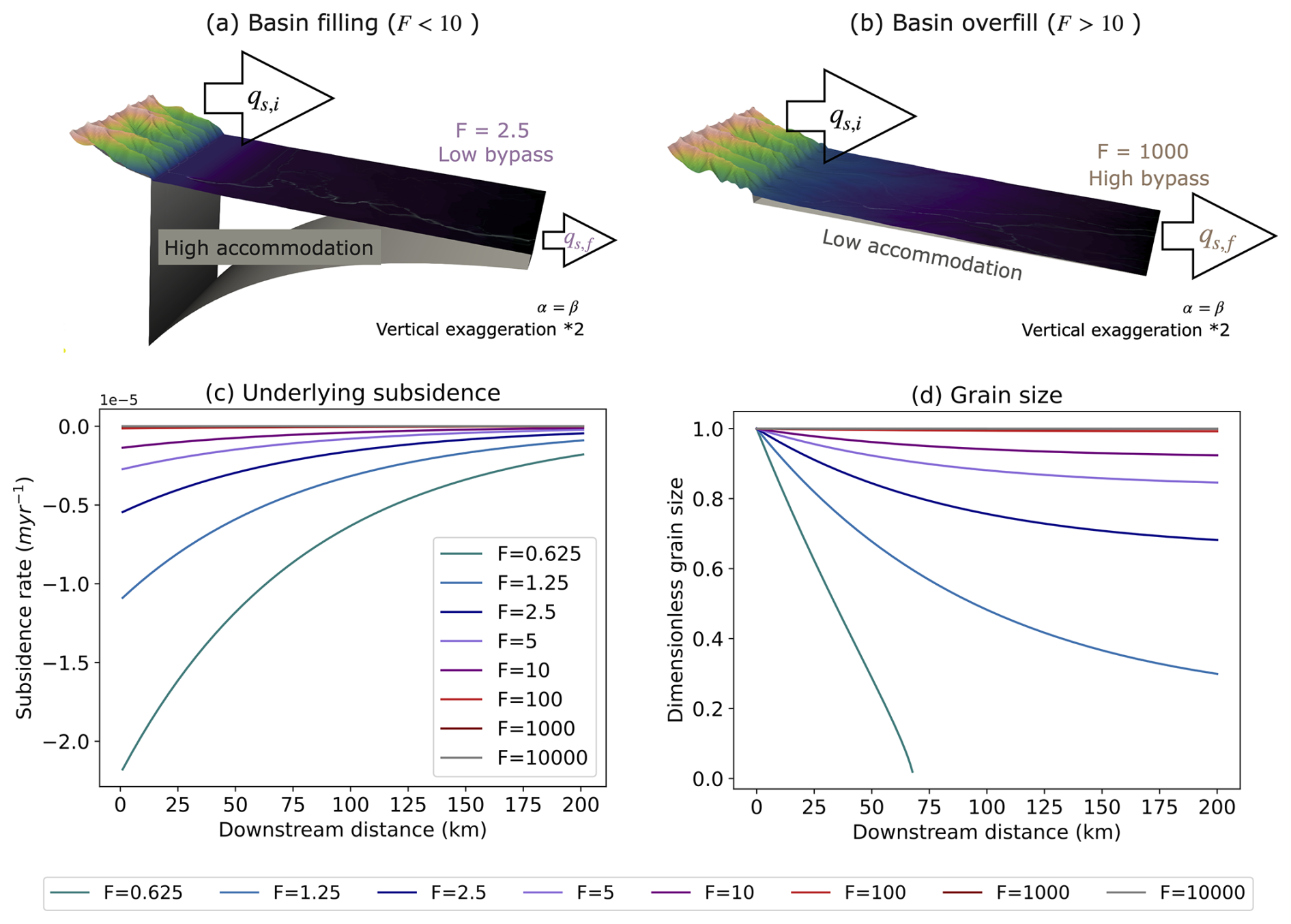
Figure 2 Examples of model runs that differ by their assumed subsidence σ₀ keeping both the incoming flux q_s,i and subsidence decay rate α constant. (a) A high subsidence value leads to a reduced outgoing flux, $q_{s_{\mathrm{f}}}$, and a smaller F=2.5 value and creates a system that is in low bypass. (b) A low subsidence value leads to an outgoing flux, $q_{s_{\mathrm{f}}}$, similar to $q_{s_i}$, and a larger F=1000 value and creates a system that is in high bypass. (c) Subsidence curve for various values of σ₀ and thus F. (d) Resulting grain size trends by varying F as obtained by Duller et al. (2010).

From the definition of the flux at steady state and by performing the integral of the subsidence given by Eq. (9), we obtain the following relationship between F, U, and σ₀:

$$\begin{array}{}\text{(11)}& F={\displaystyle \frac{(\mathrm{1}-\mathit{\gamma })U{L}_{\mathrm{M}}\mathit{\alpha }}{{\mathit{\sigma }}_{\mathrm{0}}{L}_{\mathrm{B}}(\mathrm{1}-e^{-\mathit{\alpha }})}}.\end{array}$$

In practice, we will impose values for σ₀, α, and U and deduce the corresponding value of F from Eq. (11).

Duller et al. (2010) have shown that for a given value of the incoming sediment flux from the source, q_s,i, and a given subsidence pattern, i.e. given values of F and α, the self-similar grain size fining model of Fedele and Paola (2007) predicts a unique distribution of grain size in the basin. If we note that the sediment flux at any point, x, along the surface of the basin is the upstream integral of the deposition/subsidence rate, we can substitute Eq. (9) into Eq. (3), to obtain

$$\begin{array}{}\text{(12)}& y^{*}\left(x^{*}\right)=-\ln \left(\mathrm{1}-{\displaystyle \frac{\mathrm{1}-e^{-\mathit{\alpha }{x}^{*}}}{F(\mathrm{1}-e^{-\mathit{\alpha }})}}\right),\end{array}$$

which, in turn, can be used to obtain an analytical expression for the grain size fining curve. Examples of such solutions are given in Fig. 2d. We will now compare results obtained with GravelScape with this “theoretical” solution. For this we will perform two types of model runs, one using the full two-dimensional nature of GraveScape, i.e. with a large number of nodes in the y direction, and one with only two nodes in the y direction to mimic the behaviour of a single channel. To simplify the description of the results we will use the following naming convention: the theoretical solutions (assuming deposition as equal to subsidence in a single channel) will be named DULLER; the full planform, multi-channel GravelScape solutions will be named GravelScapeMCH; and the single-channel (2 cells wide) GravelScape solution will be named GravelScape1CH. Model inputs used for standard GravelScape1CH and GravelScapeMCH setups used to validate our model against DULLER are given in Table 1.

Table 1 Reference GravelScape model parameter values for Duller validation with 1-cell orogen and imposed subsidence. Note sometimes a range of values were tested during the validation (e.g. F, G, or resolution), but the reference value has been used unless otherwise specified in the figure or caption.

4 Results: presenting GravelScape

4.1 Overview of GravelScapeMCH outputs in 2D

In Fig. 3 we show an example of the result of a GravelScape model run. We used model parameter values as given in Table 1) with an imposed subsidence producing a very high bypass basin (F=10 000) and moderately transport-limited conditions (G=1). More specifically, in Fig. 3, we show computed topography, erosion rate, drainage, grain size distribution over time (D_t), and grain size at an instantaneous time step (D_x) for a reference model experiment at a series of arbitrary consecutive time steps selected once the system has reached flux steady state; i.e. the computed values of q_s,i and q_s,f do not change significantly with time. Note that the red colours in the erosion rate map correspond to areas where net erosion takes place, whereas the blue areas correspond to areas where net deposition takes place. By comparing panels b and e, we see that GravelScape predicts instantaneous grain size (D_x) only in regions of net deposition. We see that, even though the model has reached a quasi steady state, important fluctuations in topography, discharge and grain size take place between time steps in response to what appears to be large avulsions. We note that, on average, the grain size tends to decrease from the mountain front to the base level. We also note that the predicted grain size is coarser in channels (regions of high discharge) and is highly variable spatially and temporally. Since the largest channel is often coarser than the smaller channels, the fining is greater when averaged across all channels (in the y direction) than when considering the largest channel only.

This strong variability implies (1) that the predicted grain size in the channels under high bypass should be used to compare our model's predictions to the predictions of the model of Duller et al. (2010) where predictions are limited to a single, main channel and (2) that the grain size predictions must be averaged over many time steps (e.g. >10 kyr) for comparison with the model of Duller et al. (2010), which assumes that deposition rate is equal to subsidence rate and is thus a very smooth function of x and t.

We also note that there is a small, yet non-negligible, grain size fining in the mountain area, such that the mean grain size of the material leaving the mountain front is not exactly at a value of unity, corresponding to the assumed grain size at the source. This also implies that to compare our grain size predictions to those of Duller et al. (2010), we must scale our predicted values in the basin area by the relative grain size predicted at the exit of the source area.

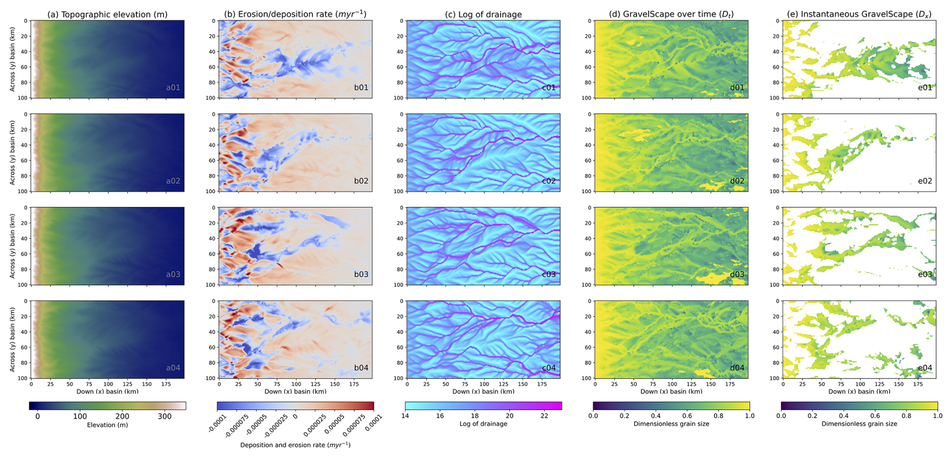
Figure 3 Steady-state predictions from GravelScape with multiple channels (2D) under high bypass (F=10 000). The four rows correspond to four successive time steps. Plan views of (a) topography, (b) erosion/deposition rate, (c) log of drainage area, (d) surface grain size updated over time (D_t), and (e) grain size (D_x) of material deposited in current time step.

4.2 Model validation and comparison to past approaches

In Fig. 4, we compare grain size predictions made by DULLER, GravelScape1CH, and GravelScapeMCH. In the top panels (a and b), we show the predicted surface and bedrock topographies obtained in GravelScapeMCH. In the middle panels (c, d, e, and f), we show the predicted grain sizes, and in the bottom panels (g and h), we show the predicted standard deposition rate for GravelScapeMCH compared to the imposed subsidence rate. In the three left panels (a, c, e, and g), we show the results of different model runs performed by varying the subsidence rate, σ₀, leading to different values of the parameter F ranging from 2.5 to 100, i.e. from low to high bypass. In the three right panels (b, d, f and h), results are shown for three values of the transport parameter G, i.e. 0.5, 1 and 1.5.

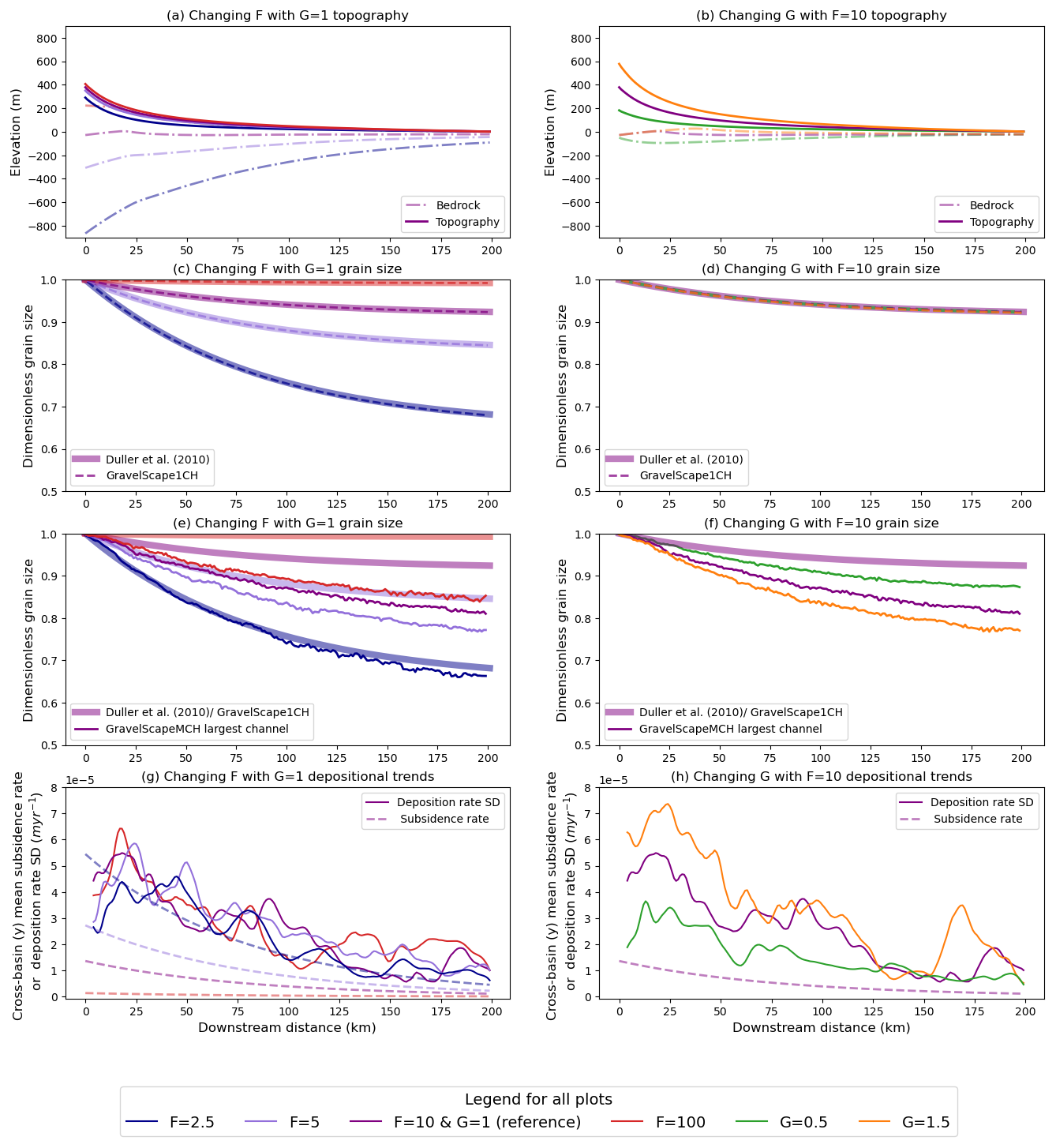
Figure 4 GravelScape model runs for different values of F (left columns varying red to blue) that represent the degree of bypass of the system and G (right columns varying green to orange) that alters the topographic profile. Panels (a) and (b) show predicted topography (solid) and basement (dashed) geometry. Panels (c) and (d) depict predicted grain size fining trends, limiting the model width to single-channel conditions (GravelScape1CH as dashed lines) compared to DULLER's (solid, opaque lines) solution. Panels (e) and (f) contain predicted grain size trends for the largest channel under multiple-channel conditions (GravelScapeMCH as solid, bold lines) compared to DULLER's (solid, opaque lines) solution. Panels (g) and (h) show the standard deviation of the deposition rate as solid, bold lines and the mean subsidence rate as dashed.

We see that the GravelScape1CH predictions are, within numerical precision, identical to DULLER for all values of F and G (Fig. 4c and d), implying that when reduced to a single channel, GravelScape reproduces the predictions of the self-similar model of Fedele and Paola (2007) exactly when deposition rate is equal to subsidence rate, as done by Duller et al. (2010). Conversely, the GravelScapeMCH predictions deviate markedly from DULLER, and the difference between the two model predictions increases with F (Fig. 4e) and G (Fig. 4f). With a constant G=1, we tested additional high bypass values of F=10–10 000 and observed the similar fining trends as the F=100 scenario in Fig. 4e. For values of roughly F>10, GravelScapeMCH predictions converge to a total grain size fining across the basin of approximately 15 % (i.e. from 1 to 0.85 in relative grain size) regardless of the value of F, whereas DULLER predicts less and less fining as F increases to the point where for F=100, there is almost no fining across the basin. Similarly, varying G (with a constant F value) in GravelScapeMCH leads to grain size fining that is 2 to 3 times larger compared to DULLER (or GravelScape1CH).

We also see that varying F has little to no effect on the surface topography at steady state (Fig. 4a), whereas changing G strongly affects it (Fig. 4b). This is because, for values of F⪆1, the surface topography is set by surface processes almost regardless of the basement subsidence as shown in Braun (2022). G, on the other hand, affects the distance over which deposition takes place and therefore strongly influences the height and slope of the depositional system (Eq. 20 in Braun, 2022). We also see that varying G causes variations not only in predicted surface topography but also in the standard deviation in deposition rate within the multi-channel model (Fig. 4h), implying that steeper sedimentary systems are affected by higher-amplitude spatial variations in deposition rate. Recall that deposition rate is a direct parameter within the Fedele and Paola (2007) equations such that any changes in deposition rate will be reflected in grain size fining.

We can therefore conclude that the deviations in grain size fining from DULLER observed in GravelScapeMCH are related to the degree of bypass of the system, when varying F, or to the shape of the surface topography changing the variation in deposition rate, when varying G. Further analysis on the internal dynamics of the system is conducted in Wild et al. (2025b).

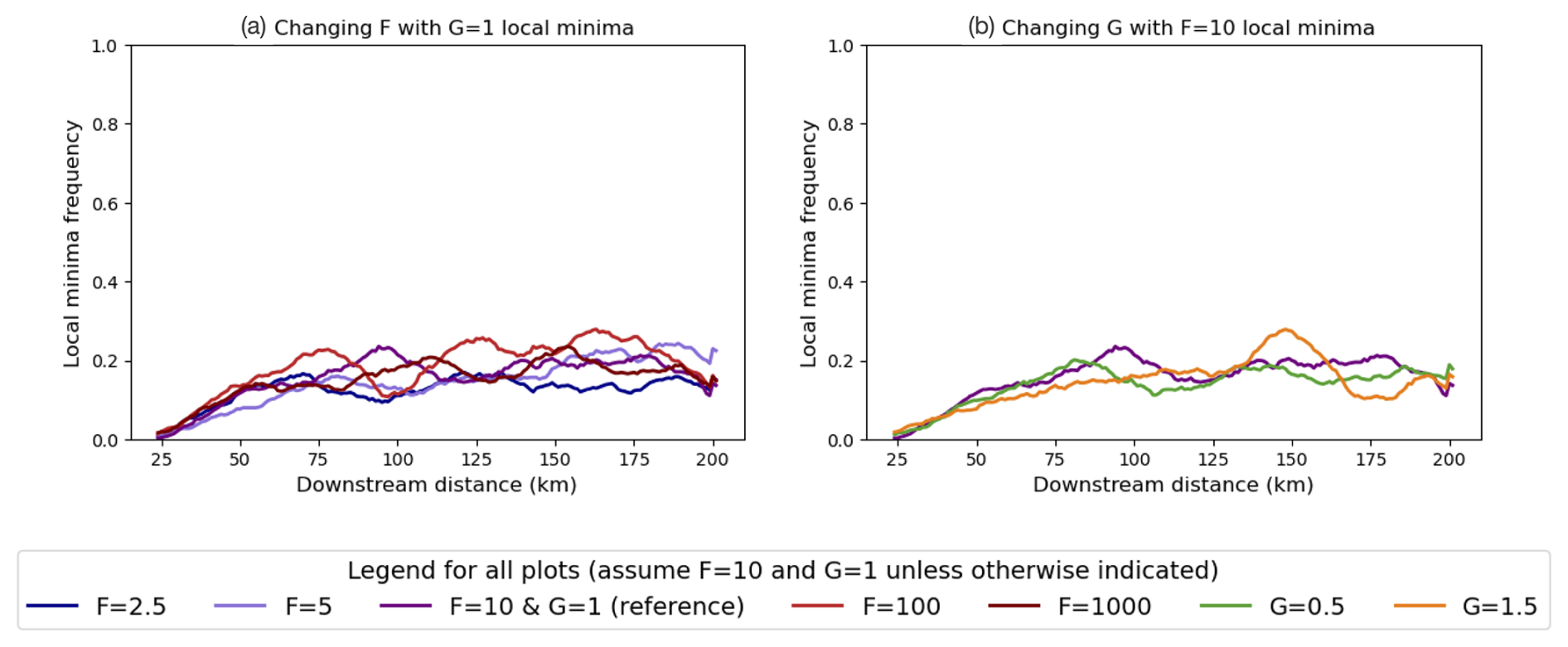
4.3 Effect of local minima

Using GravelScape with values of F<1.25 leads to predicted surface geometries that are so flat (less than a few tens of metres over a 200 km distance) that local depressions appear in the topography that lead to the formation of lakes where the modified SPL equation cannot be used to predict deposition or erosion. In the depressions, the SPL is replaced by a simple depression filling algorithm, and the resulting deposition rate cannot be used to compute grain size fining according to Eq. (1). We checked that these local depressions or minima do not influence our findings by computing the frequency of occurrence of such minima. This frequency is computed by counting the number of local minima in the main channel at a given position x over N time steps and dividing it by N−1. We found that the number of local minima is negligible for all model runs where F>1.25. In Fig. 5 we show the computed frequency of the local minima as a function of the x coordinate for the model runs shown in Fig. 4. We see that this frequency varies with the amplitude of the topography but also that it remains relatively low and does not vary significantly between the different model runs shown in Fig. 4.

Figure 5 Computed local minima frequency for the GravelScapeMCH model runs shown in Fig. 4.

4.4 Changing spatial and temporal resolution

We performed another set of model runs to verify the sensitivity of GravelScapeMCH to the assumed spatial and temporal resolution as well as the timescale over which the results are averaged to compute the grain size that we compare to DULLER. The results are shown in Fig. 6. In panel a, we see that the grain size fining computed by GravelScapeMCH depends on the spatial resolution but that the results converge with increasing resolution. This mesh dependence is related to the mobility of channels that strongly affects the standard deviation in deposition rate. We will discuss this point in greater detail in the discussion. We also see that there is little dependence of the solution on the temporal resolution (value of the time step, Δt – panel b) or on the timescale over which the grain size is averaged in GravelScapeMCH to be compared to DULLER, whether we perform this averaging over 5 Myr but with a varying number of time steps (panel c) or over 25 time steps of varying length (panel d), as long as this timescale remains larger than a characteristic timescale for channel avulsion (≈250 kyr).

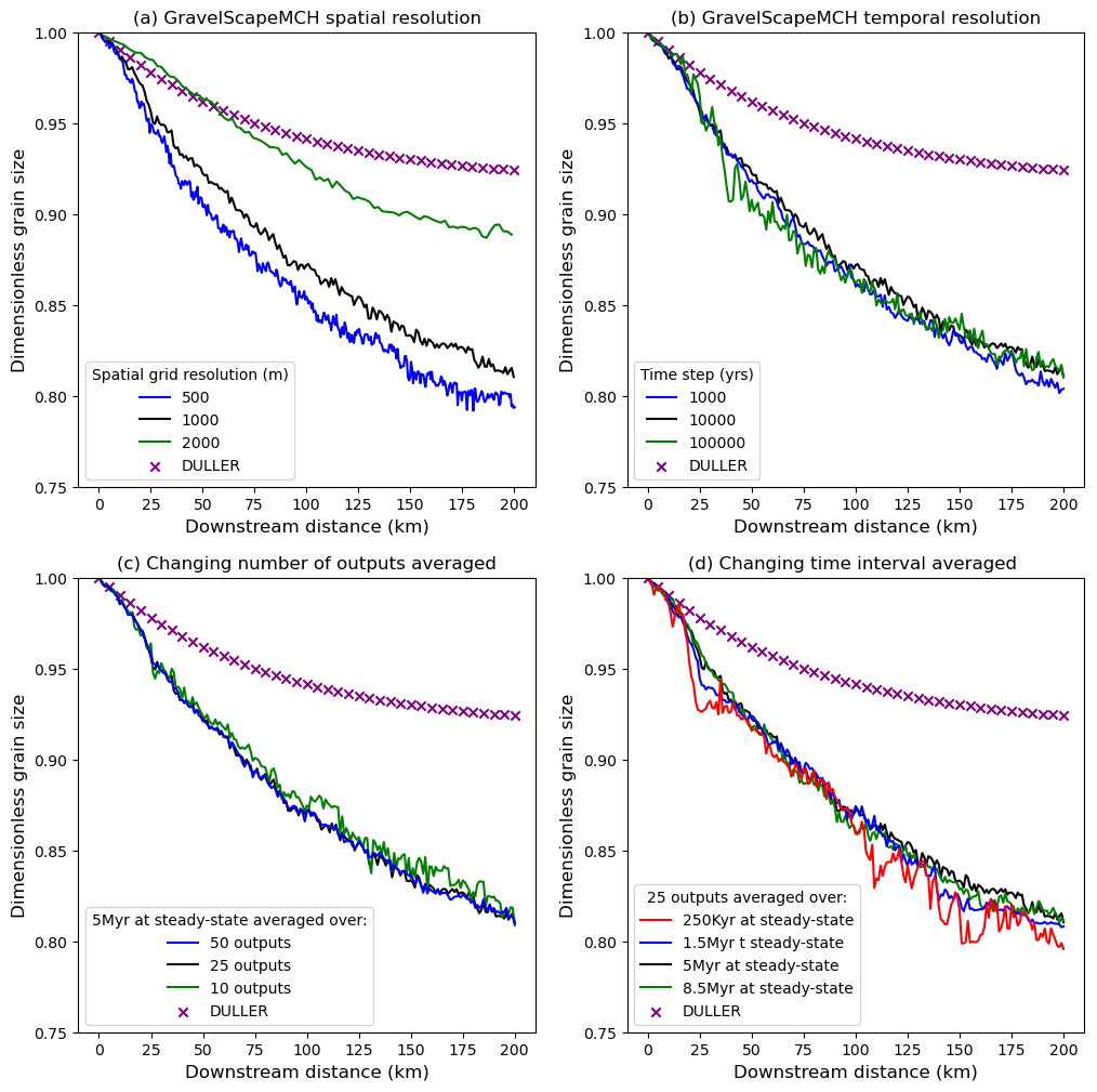
Figure 6 Effect of varying the spatial and temporal resolution in GravelScape for a moderately high bypass F=10 and G=1 setup: (a) varying spatial resolution Δx and Δy, (b) varying temporal resolution Δt, (c) varying the number of times steps used to average the solution at steady state over 5 Myr, and (d) varying the length of time used to average the solution at steady state over 25 time steps.

5 Discussion

Gravel1CH can match the simple theoretical fits of DULLER, but we have also seen from the results presented above that grain size fining trends predicted by GravelScapeMCH differ markedly from DULLER, although both models are based on the self-similar grain size fining model of Fedele and Paola (2007) that assumes that fining is controlled by deposition rate (scaled by surface sediment flux). Two main differences can be identified between the two models. First, DULLER assumes that deposition rate is equal to subsidence rate, while GravelScapeMCH computes deposition rate from an independent equation, namely the modified SPL or Eq. (6). Second, in GravelScapeMCH, solving the SPL equation provides an estimate of the surface topography that seems to influence the fining, independently of the value of the imposed subsidence rate.

The most likely reason for the difference in grain size predictions between the two models is that, in GravelScapeMCH, although mean deposition rate must be equal to the imposed subsidence rate, local deposition rate is never equal to subsidence rate due to across-basin variation (SD) (see Fig. 4g and h). This is relatively easy to demonstrate if we look at the contour maps of deposition/erosion rate in Fig. 3 that show great variability in that rate. More importantly, areas where grain size is computed correspond to areas of net deposition. This implies that grain size is, on average, computed in areas where deposition rate is larger than subsidence rate, as the mean deposition rate must be equal to the subsidence rate. This explains why, in a model, where deposition is restricted to narrow channels, the rate of fining must be greater in these channels than in the adjacent areas that experience less deposition or even erosion. This explains qualitatively why GravelScape predicts faster fining trends than the model of Duller et al. (2010) when the multiple-channel dynamics is included (GravelScapeMCH) but similar fining trends when a single channel is imposed (GraveScape1CH).

The results from our validation (Fig. 4) indicate that single-channel solutions are most applicable under more uniform flow and early basin filling states (low F), where our GravelScape multi-channel solution showed little deviation. Such is likely the case in the Pobla Basin, Montsor Formation where Duller et al. (2010) applied the Fedele and Paola (2007) grain size fining model assuming subsidence is equal to deposition rate. The Montsor Formation is described as a progradation of extensive alluvial fans filling a wedge top basin during a period of intense thrust activity and subsidence in the Southern Pyrenees Axial Zone (Duller et al., 2010). However, a more complex, multi-channel, lateral model that decouples deposition from subsidence rate is justified, if not necessary, to simulate grain size in systems with high bypass (high F), with steeper topography, or with more diverse geomorphology and stratigraphy (e.g. variations in channel dynamics, fan, and floodplain).

Additional factors (e.g. slope) that influence grain size fining in alluvial fans aside from subsidence and mean deposition rate have long been debated in the literature (Stock et al., 2008). The difference between local deposition rate and subsidence rate led D'Arcy et al. (2017) to introduce a correction factor to the model of Duller et al. (2010) to interpret grain size data from two fans systems in Death Valley. To match the observed grain size trend, they multiplied the subsidence rate by the width of the fan as a function of distance from the fan apex. In doing so, they implicitly acknowledged the difference between deposition rate in the fan active channel and the mean, across-fan, deposition rate or the fact that to create the fan, channels have to move across it and therefore locally match the subsidence rate with a deposition rate that is inversely proportional to the frequency at which the channel covers any given point of the fan surface. The correction factor of D'Arcy et al. (2017) is one example that justifies the need for our multi-channel grain size model that predicts lateral depositional variations, especially in systems where grain size fining cannot easily be explained through subsidence alone.

In GravelScape, this difference in deposition rate, and thus in grain size fining rate, between active channels and other parts of the depositional system, is taken into account “dynamically”, as we compute the local variations in deposition rate from the modified SPL equation. This approach not only is based on a better physical (and mathematical) representation of intra-basinal processes but also yields estimates of the spatial grain size variability (between channels and interfluves) and thus an estimate of the temporal variability in grain size within a given stratigraphic section.

The relationship between grain size fining and surface topography is less obvious to decipher. We see (Fig. 4h) that as G increases and the topography becomes steeper, the amplitude of the variations in deposition/erosion rate also increases. Yet, the self-similar model of Fedele and Paola (2007) that we have incorporated in GravelScape does not explicitly use the shape of the surface topography to compute grain size fining, so the link that we evidence in Fig. 4f between surface topography and grain size fining must be indirect and is, therefore, in our opinion, also related to the difference in local deposition rate between the two models as shown in Fig. 4h. This topographic influence on grain size implies that factors that can increase topography, such as initial topography or certain basin geometries, could impact the grain size fining when multi-channel solutions are considered. This warrants further study that we present in Wild et al. (2025b), along with further applications of the multi-channel model.

Computing the surface topography as done in GravelScape also provides additional constraints when inverting grain size data. As shown by D'Arcy et al. (2017), observed grain size fining trends are often affected by a strong local spatial variability in grain size, which limits our ability to unequivocally determine the shape of the subsidence function. In other words, inverting grain size data usually leads to a trade-off between σ₀ and α. Using GravelScape, topographic information can be used as an additional constraint that must be satisfied by the model, potentially resolving the trade-off between σ₀ and α. This statement must, however, be tempered down by two considerations. First, as we have shown above, topography is only sensitive to subsidence rate when F⪅5. Second, the shape of the surface topography is dependent on other, poorly constrained parameters that have been introduced in the modified SPL, such as G or K. These findings add a new dimension to our understanding of grain size fining trends in sedimentary systems and to our use of grain size data to extract from the stratigraphic record useful information about past tectonic or climatic events.

6 Conclusions

We have incorporated the self-similar grain size fining model into a plan-view landscape evolution model. We named the resulting coupled model GravelScape. Results show that although our model can reproduce the solutions of Duller et al. (2010), when the assumption of a single channel, where deposition equals the subsidence rate, is removed, GravelScape results differ and can show higher fining. The difference arises from local departures in deposition rate from the imposed subsidence rate that arise from the channelized nature of the water flow and sediment transport as predicted by GravelScape. We have demonstrated that these local variations in deposition rate lead to a more rapid fining trend across the sedimentary system and should therefore be considered when interpreting grain size data. We have also demonstrated that the amplitude of grain size deviation from the single-channel solution depends on the value of the bypass parameter F. As F increases, the differences between the GravelScape predictions and those from the one-dimensional model increase to the point where for values of F larger than 100, grain size fining becomes independent of F. We have also shown that topography appears to control fining through the parameter G, where steeper topographies produced greater depositional variation across the basin and more deviation from the single-channel fining solutions. It also appears that these deviations in predicted grain size fining rate predicted by GravelScape (compared to single-channel models) are in proportion to the standard deviation in deposition rate caused by channel avulsions and deposition/incisional pulses within the landscape.

These findings demonstrate the need to better understand what controls the amplitude and frequency of fluctuations in sedimentation rate. This is our objective in the second paper (Part 2, Wild et al., 2025b) where we define the conditions under which grain size fining is principally controlled by subsidence or by internal processes in a quantitative manner.