At-a-site and between-site variability of bedload transport, inferred from continuous surrogate monitoring, and comparison to predictive equations

This study investigates spatial and temporal variability of bedload transport in four Swiss mountain streams using continuous Swiss Plate Geophone (SPG) monitoring. This surrogate measuring system had been calibrated in previous studies to produce reliable estimates of bedload transport rates. The measurements were analysed at two different time scales: short-term transport events typically covering a duration of a few weeks and multi-year annual transport totals. Power-law relations between dimensionless transport intensity and shear stress were derived to evaluate the temporal variability in the steepness of transport relations and in the reference shear stress. Results were compared with predictive equations developed for mountain streams. Findings show substantial variability both within and across sites, likely reflecting the influence of sediment availability, stream slope, streambed texture and flow history. Overall, continuous monitoring highlights the strong role of temporal spatial variability on bedload transport levels, possibly due to changing sediment availability and bed surface composition, and with implications for predictive modelling and river management.

1 Introduction

Traditionally, bedload transport has been modeled using semi-empirical relations between mean transport and mean hydraulic variables such as shear stress or flow discharge (Bagnold, 1966; Meyer-Peter and Müller, 1948; Recking, 2013; Schneider et al., 2015a; Wilcock and Crowe, 2003). However, extensive field measurements and flume experiments have demonstrated that bedload transport is often highly variable at multiple spatial and temporal scales. Many reasons for the variability were listed by Ancey (2020), and they include the mixing of fast and slow processes, nonequilibrium and noise-driven processes, cascades of interacting processes, varying temporal and spatial scales dependent on flow conditions, heterogeneity of materials and flow conditions, nonlinearity and threshold effects, and poor knowledge of initial and boundary conditions.

One of the most important elements of variability is the threshold of motion. The critical Shields number (e.g., Buffington and Montgomery, 1997) describes a critical dimensionless shear stress for particle entrainment. However, observations have shown that individual grains move both below and above the predicted threshold due to turbulence, grain protrusion, and intergranular force chains (Nelson et al., 1995; Diplas et al., 2008). Particle motion reflects stochastic impulses, resulting in intermittent entrainment. Laboratory studies confirm that impulse duration and magnitude are more predictive than mean shear stress (Valyrakis et al., 2010).

Memory effects or history dependence can affect bedload transport variability. For example, the threshold for motion is influenced by factors such as flow duration, prior high or low flows, and disturbance of the bed (by floods or large transport events). In low-flow or inter-event periods, the bed surface stabilizes (settlement, compaction), thereby increasing the entrainment threshold, observed both in flume experiments and for example in the Swiss Erlenbach stream (Masteller and Finnegan, 2017; Masteller et al., 2019). Conversely, at higher flows with important sediment supply to and deposition on the channel, observations at the Erlenbach showed a decrease of the entrainment threshold (Rickenmann, 2020, 2024). In mixed-size sediments, bed-surface structure produces partial transport, whereby only a fraction of the surface is mobile at a given flow (Wilcock and McArdell, 1993; Parker, 2008). Surface armoring shields finer grains and creates patchy mobility, while coarser clasts may move only episodically during high flows (Church, 2006; Turowski et al., 2009; Vázquez-Tarrío et al., 2020). This selective mobility introduces large variability into fractional bedload rates. Bed shear stress is not spatially uniform but dominated by coherent turbulent structures. Bursts, sweeps, and vortices impart localized impulses capable of mobilizing grains otherwise at rest (Nelson et al., 1995; Schmeeckle and Nelson, 2003; Dwivedi et al., 2011).

Evolving bedforms and morphological structures (e.g., ripples, dunes, alternate bars, step-pool structures) contribute to temporal and spatial variability by alternately storing and releasing sediment (Vázquez-Tarrío et al., 2020). Migrating bedforms and structures impose oscillations in transport at timescales linked to bedform wavelength and celerity (Gomez et al., 1989) and to strong flow events capable of destroying step-pool structures (Golly et al., 2017). Bed topography also generates localized roughness, further amplifying spatial heterogeneity in transport rates (Monsalve et al., 2020). Phase-1 bedload transport typically involves finer grains and is controlled more by upstream sediment supply and availability than by water discharge; in contrast, phase-2 bedload transport shows a clear dependence on water discharge, and particles from the bed surface layer are also likely to be mobilized (Church, 2010; Rickenmann, 2018; Warburton, 1992).

Bedload variability also reflects external forcings such as landslides, debris flows, and tributary inputs. Such pulses of material supply can temporarily overwhelm the transport capacity, creating surges of bedload independent of discharge (Lisle et al., 1997). Experimental evidence shows that episodic sediment supply increases variability, especially at longer timescales (Elgueta-Astaburuaga et al., 2018). Hydrograph dynamics further amplify variability: in perennial streams transport often peaks disproportionately on the rising limb relative to falling stages due to supply exhaustion and channel adjustments (Pretzlav et al., 2020; Mao et al., 2019; Rickenmann, 2024), whereas in ephemeral streams typically lacking an armour layer such as the Nahal Eshtemoa no clear hysteresis pattern could be found for the majority of the flood events (Cohen et al., 2010).

Recking et al. (2016) compiled bedload transport measurements from more than 100 streams with the goal to study how river bed morphology (such as step-pool, riffle-pool, braiding, plane beds, sand beds) influences fluvial bedload transport rates. They used a standard bedload transport equation as a function of shear stress as a reference situation, whereby this equation (Recking, 2013) was developed in such a way that it can be linked to bedload measured in narrow flumes in the absence of any bed form. They applied a generalized form of the equation to the many streams, varying either the exponent (steepness) of the bedload transport relation for the steep part of the equation or the reference shear stress, to find a good agreement of the predictions with the measurements. Both the steepness and the reference shear stress have generally a large effect on the predicted bedload transport level, and the study found that both optimized variables varied in a considerable range. Furthermore, Recking et al. (2016) showed that the optimal steepness (exponent) varied somewhat with channel geometry and bedform type, and that the optimal reference shear stress strongly depended on channel slope. They concluded that only narrow natural channels, especially those with plane beds, behave like a flume, while larger rivers deviate more from the flat-bed flume situation. For riffle-pool morphologies, they further found a grain-size distribution effect, likely a proxy for the riffle-pool development, on the optimal reference shear stress.

Until about two decades ago, direct bedload measurements were the main means to quantify its variability in natural streams. However, most of these measurements suffered from the important limitation that typically only discrete samples were taken in time and space (in a given cross-section), and sampling at higher flows was often not feasible. After about 2005, more and more surrogate bedload systems with impact plate geophones were installed in gravel-bed streams (Coviello et al., 2022; Rickenmann, 2017; Rickenmann et al., 2022; Rindler et al., 2025). These indirect measurements have the advantage of a continuous monitoring of bedload transport, typically using a 1 min recording interval, and of including also higher flows.

Rickenmann (2018) analyzed measurements with Swiss plate geophones (SPG) from 6 years in the two glacier-fed mountain streams Fischbach and Ruetz in Austria. He observed that an exponential form of the Meyer-Peter and Mueller (MPM) equation (Cheng, 2002) could reasonably well represent the increase in bedload transport with discharge for phase-2 transport conditions. A back-calculation of appropriate critical Shields numbers (which are similar to dimensionless reference shear stresses for the exponential MPM form) showed seasonal and year-to-year fluctuations, with the Shield values mostly ranging from 0.01 to 0.06. In these calculations, an effective or reduced shear stress was used together with the exponential MPM equation. In the same study, Rickenmann (2018) found that correlation between bedload transport rates and discharge considerably increased, if these values were aggregated over about 1 to 2 h. This finding may be associated with fluctuations of bedload transport with a periodicity of 14–35 min observed both in natural streams and in flumes for a variety of hydraulic conditions and sediment supply, possibly due to moving bed load sheets or the formation and destruction of gravel clusters (Rickenmann, 2018). Observations from the Erlenbach stream with the SPG system showed that disequilibrium ratio of measured to calculated transport values influenced bedload transport behavior (Rickenmann, 2020, 2024). Above-average disequilibrium conditions, which were associated with a greater sediment availability on the streambed, generally had a stronger effect on subsequent transport conditions than below-average disequilibrium conditions, which were associated with comparatively less sediment availability on the streambed.

Coviello et al. (2022) also used an impact plate geophone system and considered longer-term fluctuations of bedload transport. They analyzed seven years of bedload data in the glacier-fed Italian Sulden stream and found that climatic factors (snow cover and temperature) modulate bedload flux seasonally and inter-annually. They also found that, for the same discharge in different seasons, transport rates can differ markedly. Kreisler et al. (2017) measured bedload transport with impact plate geophones at the Urslau torrent in Salzburg. They analyzed three years of data including more than 30 individual bedload-transporting flood events and found that bedload transport efficiency, defined as the ratio of observed bedload transport to excess stream power, varied considerably among different events and across years. Their study also showed that variable sediment supply conditions affected the prevailing bedload transport rates at the Urslau stream. Aigner et al. (2017) used impact plate geophone measurements over a 15-year period in the Upper Drau River in Austria, obtained from instruments installed 2 km downstream of a reach with only residual flow, due to the existence of an upstream hydropower plant. Their analysis revealed a complex process of gravel storage and intermittent re-supply from the residual upstream reach. Frequently occurring bedload pulses produced very high bedload fluxes while in transit and tended to increase bedload flux in the post-event phase, and could alter and reduce the sediment storage in upstream reaches, leading to a reduction in bedload availability for future pulses.

The goal of this study is to quantify the variability of bedload transport in detail in four mountain streams in Switzerland, as inferred from continuous measurements with the SPG system, for two different time scales. The first analysis addresses the temporal variability of bedload transport for a given year, where active periods of bedload movement typically occurred in the summer half-year in the four streams. The variability is quantified by determining power law relations between transport rates and shear stresses, for the steep part of the transport relations (phase-2 transport conditions), and typically over successive two-weeks periods. The resulting power law equations allow to determine the steepness of the bedload rating curve and to infer a corresponding reference shear stress. This analysis permits a comparison and discussion with the comprehensive study of Recking et al. (2016) that considered the between-site variability of the same two variables (steepness and reference shear stress) for a large data set including direct bedload measurements, mentioned above. The second analysis aims to compare calculated and observed bedload masses summed up over individual years, considering extended data sets for the same four Swiss streams with typical observation durations of several years.

2 Observation sites, bedload transport equations and analysis

2.1 Observation sites, SPG calibration, and discharge data

Measurements with the SPG System have been obtained in five Swiss mountain streams over several years (e.g. Rickenmann et al., 2022; Schneider et al., 2016; and further references in Table 1). Here I first compare one-year measurements from these five streams (Table 1) with four bedload transport equations. The main stream characteristics necessary for the bedload transport calculations are also listed in Table 1. For all of these streams, calibration relations were already discussed in Antoniazza et al. (2022), Rickenmann et al. (2012), Nicollier et al. (2021, 2022), and Schneider et al. (2016). The location of the five SPG sites is shown in Fig. 1. For the further analysis as described in Sect. 2.3 and 2.4, only four streams were considered, the Riedbach was excluded due to the limited time resolution of the SPG data.

Table 1 Characteristics of Swiss field sites with SPG measurements. A_c = catchment area, Q_max = maximum discharge for the observation year, w = channel width, S = channel slope, D_xx = characteristic grain size (see also text and Appendix E).

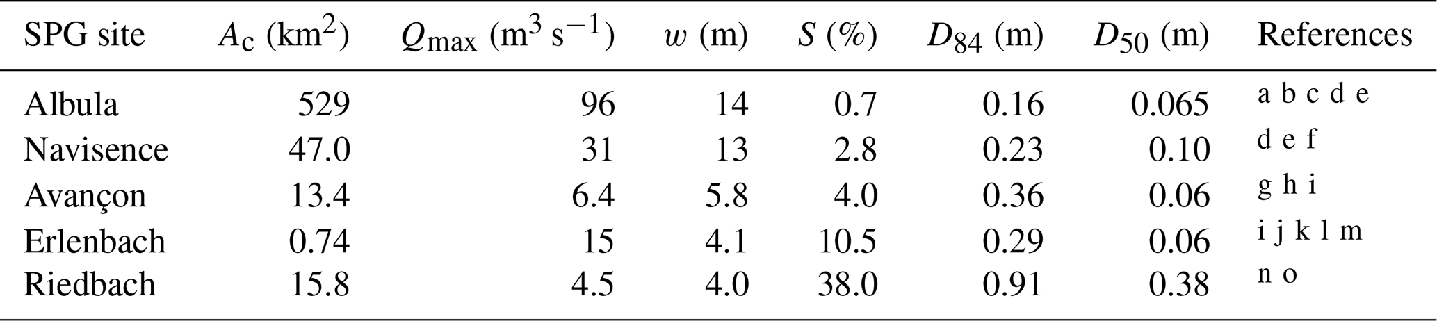
^a Rickenmann et al. (2017), ^b Nicollier et al. (2019), ^c Rickenmann et al. (2020a), ^d [4] Nicollier et al. (2021), ^e Nicollier et al. (2022), ^f Nicollier et al. (2020), ^g Antoniazza et al. (2022), ^h Antoniazza et al. (2023), ⁱ Rickenmann et al. (2022), ^j Rickenmann and McArdell (2007), ^k Rickenmann et al. (2012), ^l Rickenmann (2020), ^m Rickenmann (2024), ⁿ Schneider et al. (2015b), ^o Schneider et al. (2016).

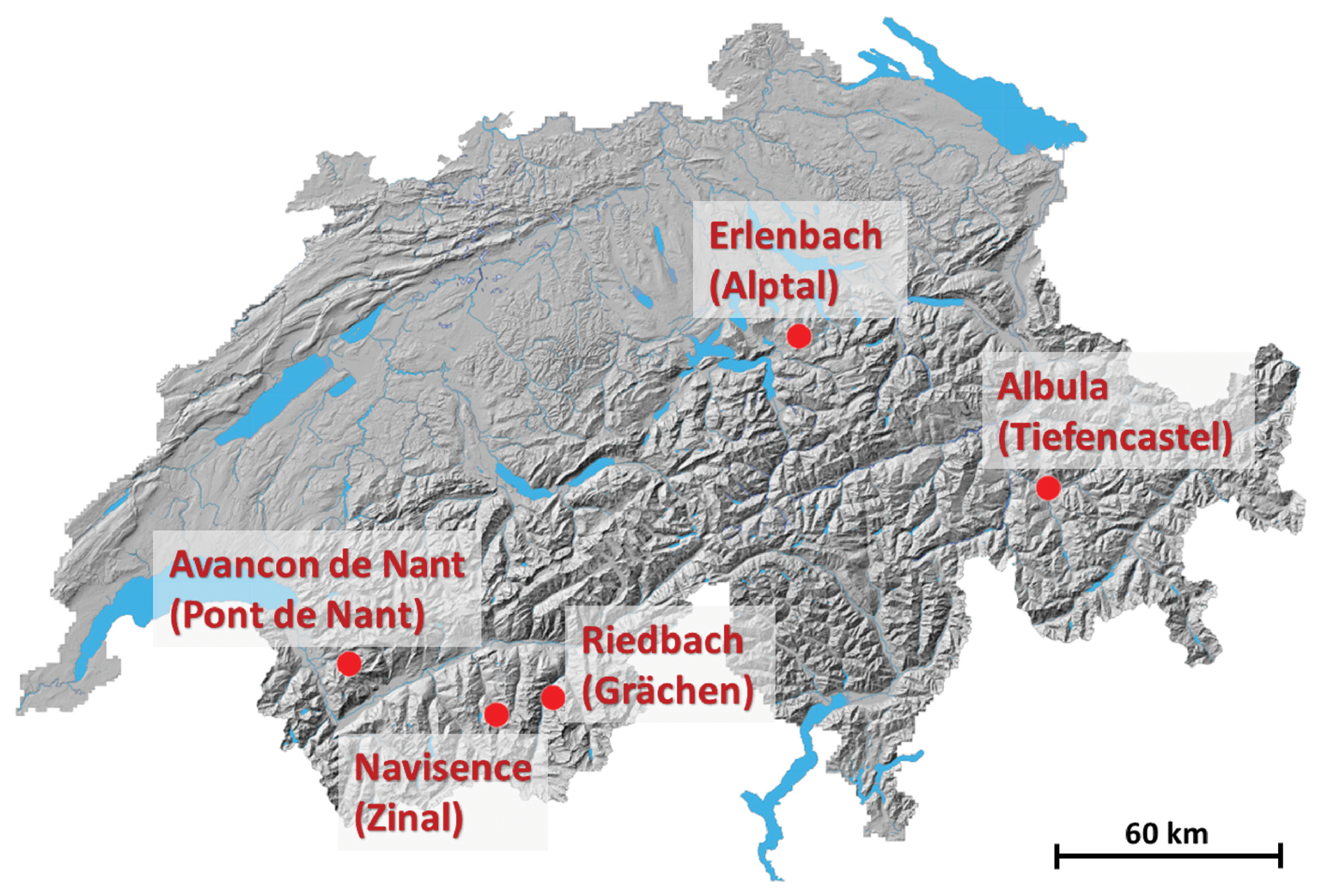
Figure 1 Field sites in Swiss streams with SPG measurements.

The SPG System recorded summary values including impulses (IMP) for 1 min intervals at the first four sites in Table 1, whereas IMP values were stored only for 10 min intervals for the Riedbach stream. For this study, new calibration relations were defined for the three streams, namely for the Albula, the Navisence, and the Avançon, according to the following equation:

$$\begin{array}{}\text{(1)}& M=k_{\mathrm{site}}\mathrm{IMP}\end{array}$$

For the calibration, M = measured bedload mass (in kg, for grain size D > 9.5 mm), k_site = linear calibration coefficient with the units (kg), and IMP = sum of impulses recorded over 1 min intervals. These calibration coefficients were reported in Baldig and Rickenmann (2024). For the Erlenbach, the linear calibration coefficient varied according to the survey periods of the deposited sediments in the retention basin (Rickenmann, 2020, 2024), and for the Riedbach a power-law calibration relation was determined (Schneider et al., 2016). The calibration coefficients and equations used in this study for the different SPG sites are summarized in Table 2. The measured bedload transport rate Q_b (in kg s⁻¹) was derived by dividing the transported bedload mass by the respective recoding time interval in seconds, and it represents the total bedload discharge over the entire stream width.

Table 2 Calibration coefficients and equations used for the different SPG sites. The calibration coefficient k-isp for the Erlenbach refers to individual survey periods of the sediment deposits in the retention basin.

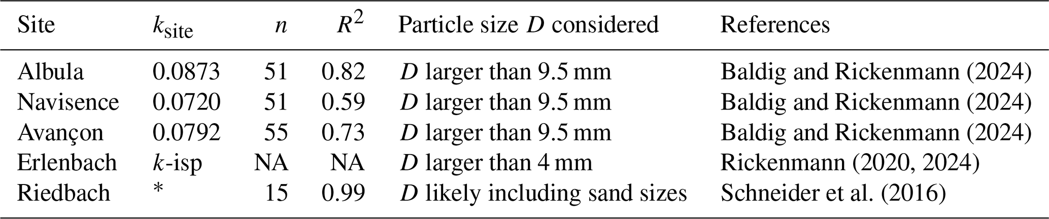
^∗ A power law calibration equation was used for the Riedbach.

For the Erlenbach, for 12 flood events basket samples were available with information regarding transported grain sizes in the range of 4 mm < D < 10 mm (see also Table 2). Based on these data, a mean coefficient m_fg = 1.54 was estimated, to multiply the mass M in Eq. (1) to account for this fine fraction undetected by the SPG system, and applied to the Erlenbach measurements (Rickenmann, 2024). For the individual basket samples, the coefficient m_fg varied between about 1.4 and 1.9, with a tendency to decrease for increasing total transport rates Q_b in the range of about 0.02 to 0.8 kg s⁻¹. For the Albula, Navisence, and Avançon, no such information was available, so for these streams no correction was applied. For the Riedbach, the calibration relation of the SPG system considered also fine material deposited in the settling basin of the water intake, and therefore likely included also some sand sized particles (Schneider et al., 2016). For the later comparison with bedload transport equations it would be more correct to also account for the fraction of particles in the range of fine gravel, i.e. for 4 mm < D < 10 mm. However, given the large variabilities of bedload transport rates often extending over one or more orders of magnitudes and the goals of this study, this uncertainty about partly lacking information on finer transported bedload particles may be considered acceptable. The general uncertainty of the SPG system was discussed and quantified for four Swiss stream sites in Rickenmann et al. (2024a, b).

Observations of bedload transport often show a large variability for a given discharge value, typically covering several orders of magnitudes. In such a situation, when binning the measurements into discharge classes to determine a mean trend of the observed transport rates, it is preferable to calculate the geometric mean of the Q_b values. However, this brings about the problem of how to deal with observed zero Q_b values. Here, I took an approach similar to that proposed by Gaeuman et al. (2009, 2015), averaging the zero Q_b=Q_bz values with (temporally) neighboring non-zero Q_b values. I replaced the Q_bz values by averaging any k successive Q_bz values by including the two neighboring non-zero Q_{bz_p} and Q_{bz_a} values, where the indices stand for p = prior and a = after a series of k successive Q_bz values. Then I assigned to all (k+2) values the average value $Q_{\mathrm{bM}}=(Q_{\mathrm{bz}\mathrm{\_}\mathrm{p}}+Q_{\mathrm{bz}\mathrm{\_}\mathrm{a}})/(k+\mathrm{2})$. This procedure was previously applied to the Erlenbach bedload measurements (Rickenmann, 2024). Thus, contrary to the Q_b values that include zero values, all the Q_bM values are non-zero and a representative geometric mean value can be calculated for a given discharge class.

At four sites (Navisence, Avançon, Erlenbach, and Riedbach) discharge measurements of Q (in m³ s⁻¹) were available at the location of the SPG measurements (see references in Table 1). At the Albula river in Tiefencastel, a runoff gauging station is located a few hundred meters downstream of the SPG site. These discharge data were corrected for bypassed water used by a hydropower company and returned to the river in the reach in-between the two sites (Rickenmann et al., 2017).

2.2 Flow resistance calculations and bedload transport equations

The flow-resistance and the bedload-transport calculations were made four all five streams as described in Rickenmann (2020, 2024) for the Erlenbach. They were based on the measured trapezoidal cross-section in the natural reach upstream of the SPG measuring installations. Characteristic grain sizes D_xx, channel bottom width w, and channel slope S are given in Table 1; D_xx is the grain size for which xx % of the particles by mass are finer. The flow-resistance calculations were made with a hydraulic geometry flow resistance relation developed by Rickenmann and Recking (2011), and they are summarized in Appendix A.

Similar as for the Erlenbach (Rickenmann, 2020, 2024), the bedload-transport calculations were performed using two equations reported in Schneider et al. (2015a), which represent a modified form of the Wilcock and Crowe (2003) equation and predict total bedload transport rates (not fractional transport rates) for grain sizes larger than 4 mm. The first one (SEA1) is based on the use of total shear stress and a slope-dependent reference shear stress:

$$\begin{array}{}\text{(2a)}& {\displaystyle }\begin{array}{rl}& W_{\mathrm{tot}}^{\ast }=\mathrm{0.002}{\left({\displaystyle \frac{{\mathit{\tau }}_{D_{\mathrm{50}}}^{\ast }}{{\mathit{\tau }}_{\mathrm{r}{D}_{\mathrm{50}}}^{\ast }}}\right)}^{\mathrm{16.1}}\\ & \mathrm{for}{\displaystyle \frac{{\mathit{\tau }}_{D_{\mathrm{50}}}^{\ast }}{{\mathit{\tau }}_{\mathrm{r}{D}_{\mathrm{50}}}^{\ast }}}<\mathrm{1.143}\mathrm{and}D>\mathrm{4}\mathrm{mm}\end{array}\text{(2b)}& {\displaystyle }\begin{array}{rl}& W_{\mathrm{tot}}^{\ast }=\mathrm{14}{\left(\mathrm{1}-{\displaystyle \frac{\mathrm{0.85}}{{\left({\mathit{\tau }}_{D_{\mathrm{50}}}^{\ast }/{\mathit{\tau }}_{\mathrm{r}{D}_{\mathrm{50}}}^{\ast }\right)}^{\mathrm{0.7}}}}\right)}^{\mathrm{4.5}}\\ & \mathrm{for}{\displaystyle \frac{{\mathit{\tau }}_{D_{\mathrm{50}}}^{\ast }}{{\mathit{\tau }}_{\mathrm{r}{D}_{\mathrm{50}}}^{\ast }}}\ge \mathrm{1.143}\mathrm{and}D>\mathrm{4}\mathrm{mm}\end{array}\end{array}$$

where the dimensionless transport rate $W_{\mathrm{tot}}^{\ast }$ according to Wilcock and Crowe (2003) is defined as:

$$\begin{array}{}\text{(3)}& W_{\mathrm{tot}}^{\ast }=(s-\mathrm{1})g{q}_{\mathrm{b}}/u^{\ast \mathrm{3}},\end{array}$$

and where $s={\mathit{\rho }}_{\mathrm{s}}/\mathit{\rho }$ = relative sediment density, with ρ_s = sediment particle density and ρ = water density, q_b = volumetric bedload transport rate per unit width, u^∗ = ($\mathit{\tau }/\mathit{\rho }{)}^{\mathrm{0.5}}$ = shear velocity, and τ=gρr_hS = bed shear stress. ${\mathit{\tau }}_{D_{\mathrm{50}}}^{\ast }$ = $r_{\mathrm{h}}S/\left(R{D}_{\mathrm{50}}\right)$ is the dimensionless bed shear stress with regard to the characteristic grain size D₅₀, and ${\mathit{\tau }}_{\mathrm{r}{D}_{\mathrm{50}}}^{\ast }$ is the dimensionless reference bed shear stress with regard to the characteristic grain size D₅₀ of the bed surface. The threshold between low and high intensity transport in Eq. (2) has been corrected to ${\mathit{\tau }}_{D_{\mathrm{50}}}^{\ast }/{\mathit{\tau }}_{\mathrm{r}{D}_{\mathrm{50}}}^{\ast }$ = 1.143 (Rickenmann, 2024), as compared to the value of 1.2 given in Schneider et al. (2015a). ${\mathit{\tau }}_{\mathrm{r}{D}_{\mathrm{50}}}^{\ast }$ is calculated as a function of the bed slope (Schneider et al., 2015a, Eq. 10 therein):

$$\begin{array}{}\text{(4)}& {\mathit{\tau }}_{\mathrm{r}{D}_{\mathrm{50}}}^{\ast }=\mathrm{0.56}{S}^{\mathrm{0.5}}\end{array}$$

The bedload transport rate over the entire channel width Q_b (in kg s⁻¹), calculated with the total shear stress, is given as:

$$\begin{array}{}\text{(5)}& Q_{\mathrm{btot}}=w{\mathit{\rho }}_{\mathrm{s}}{W}_{\mathrm{tot}}^{\ast }{u}^{\ast \mathrm{3}}/\left(\right(s-\mathrm{1}\left)g\right)\end{array}$$

The second equation (SEA2) is based on a reduced (effective) shear stress τ^′, using a reduced energy slope S^′ (Rickenmann and Recking, 2011; Schneider et al., 2015a):

$$\begin{array}{}\text{(6)}& {\displaystyle }{\mathit{\tau }}^{\prime }=g\mathit{\rho }{r}_{\mathrm{h}}{S}^{\prime }\text{(7)}& {\displaystyle }{S}^{\prime }=S\left(f_o/f_{\mathrm{tot}}\right)S^{\mathrm{0.5}e},\end{array}$$

where e = 1.5, f_tot = friction factor for total flow resistance, calculated with Eq. (A1), and f_o = friction factor associated with grain resistance, calculated as (Rickenmann and Recking, 2011):

$$\begin{array}{}\text{(8)}& f_o=\left(\mathrm{8}/{\mathrm{6.5}}^{\mathrm{2}}\right){\left(D_{\mathrm{84}}/r_{\mathrm{h}}\right)}^{\mathrm{0.334}}\end{array}$$

The dimensionless transport rate $W_{\mathrm{red}}^{\ast }$ is determined as:

$$\begin{array}{}\text{(9a)}& {\displaystyle }\begin{array}{rl}& W_{\mathrm{red}}^{\ast }=\mathrm{0.002}{\left({\displaystyle \frac{{\mathit{\tau }}_{D_{\mathrm{50}}}^{\ast \prime }}{{\mathit{\tau }}_{\mathrm{r}{D}_{\mathrm{50}}}^{\ast \prime }}}\right)}^{\mathrm{7.8}}\\ & \mathrm{for}{\displaystyle \frac{{\mathit{\tau }}_{D_{\mathrm{50}}}^{\ast \prime }}{{\mathit{\tau }}_{\mathrm{r}{D}_{\mathrm{50}}}^{\ast \prime }}}<\mathrm{1.33}\mathrm{and}D>\mathrm{4}\mathrm{mm}\end{array}\text{(9b)}& {\displaystyle }\begin{array}{rl}& W_{\mathrm{red}}^{\ast }=\mathrm{14}{\left(\mathrm{1}-{\displaystyle \frac{\mathrm{0.894}}{{\left({\mathit{\tau }}_{D_{\mathrm{50}}}^{\ast \prime }/{\mathit{\tau }}_{\mathrm{r}{D}_{\mathrm{50}}}^{\ast \prime }\right)}^{\mathrm{0.5}}}}\right)}^{\mathrm{4.5}}\\ & \mathrm{for}{\displaystyle \frac{{\mathit{\tau }}_{D_{\mathrm{50}}}^{\ast \prime }}{{\mathit{\tau }}_{\mathrm{r}{D}_{\mathrm{50}}}^{\ast \prime }}}\ge \mathrm{1.33}\mathrm{and}D>\mathrm{4}\mathrm{mm}\end{array}\end{array}$$

For equation (SEA2) the slope-independent dimensionless reference shear stress is constant:

$$\begin{array}{}\text{(10)}& {\mathit{\tau }}_{\mathrm{r}{D}_{\mathrm{50}}}^{\ast \prime }=\mathrm{0.03}\end{array}$$

The bedload transport rate over the entire channel width Q_b, calculated with the reduced shear stress, includes the shear velocity $u^{\ast \prime }=({\mathit{\tau }}^{\prime }/\mathit{\rho }{)}^{\mathrm{0.5}}$ and is given as:

$$\begin{array}{}\text{(11)}& Q_{\mathrm{bred}}=w{\mathit{\rho }}_{\mathrm{s}}{W}_{\mathrm{red}}^{\ast }{u}^{\ast \prime \mathrm{3}}/\left(\right(s-\mathrm{1}\left)g\right)\end{array}$$

For the development of Eqs. (2) and (9), Schneider et al. (2015a) used bedload transport measurements from 14 mountain streams, including channel slopes mainly from steep streams (SS) in the range 0.01 < S < 0.11 (except for the Oak Creek with S = 0.0014). The bedload transport characteristics of these 14 mountain streams (called “main data set” in Schneider et al., 2015a) are labeled SEA_SS data in this study and compared with our results below. Similarly, data from 21 streams with Helley-Smith bedload samples (called “HS data set” in Schneider et al., 2015a) are labeled “SEA_HS” data in this study and compared with our results below.

Regarding possible overlap with the five streams listed in Table 1, basket samples from the Erlenbach (Rickenmann et al., 2012) and net samples from the Riedbach in the flat upstream reach Schneider et al. (2015b) were used in the SEA_SS data set. However, for both two streams the SPG measurements were independent of the samples analyzed in the in the SEA_SS data set by Schneider et al. (2015a).

For further comparison with other transport equations introduced below, the steep part of the bedload transport relations (Eqs. 2a, 9a) is expressed in general form as:

$$\begin{array}{}\text{(12)}& {\displaystyle }{W}^{\ast }=a{\left({\displaystyle \frac{{\mathit{\tau }}^{\ast }}{{\mathit{\tau }}_{\mathrm{ref}}^{\ast }}}\right)}^m\text{(13)}& {\displaystyle }{W}^{\ast }=(s-\mathrm{1})g{q}_{\mathrm{b}}/u^{\ast \mathrm{3}}\end{array}$$

In Eq. (12), a is a coefficient, m is an exponent, and τ^∗ and ${\mathit{\tau }}_{\mathrm{ref}}^{\ast }$ may refer to calculations with either the total shear stress (Eq. 2) or with a reduced shear stress (Eq. 9).

Another bedload transport equation by Recking et al. (2016) is used here, where Φ_b is a dimensionless transport rate:

$$\begin{array}{}\text{(14)}& {\displaystyle }{\mathrm{\Phi }}_{\mathrm{b}\mathrm{84}}=A{{\mathit{\tau }}_{D_{\mathrm{84}}}^{\ast }}^{\mathit{\alpha }}\left({\mathit{\tau }}_{D_{\mathrm{84}}}^{\ast }/\left(\mathrm{1}+{\left({\displaystyle \frac{{\mathit{\tau }}_{\mathrm{rRe}}^{\ast }}{{\mathit{\tau }}_{D_{\mathrm{84}}}^{\ast }}}\right)}^{\mathit{\beta }}\right)\right)\text{(15)}& {\displaystyle }{\mathrm{\Phi }}_{\mathrm{b}\mathrm{84}}=q_{\mathrm{b}}/\sqrt{(s-\mathrm{1})g{D}_{\mathrm{84}}^{\mathrm{3}}}\text{(16)}& {\displaystyle }{\mathit{\tau }}_{D_{\mathrm{84}}}^{\ast }=r_{\mathrm{h}}S/\left(\right(s-\mathrm{1}\left)D_{\mathrm{84}}\right),\end{array}$$

where A is a coefficient, and α and β are exponents. For the general comparison with measured Q_b values of the Swiss streams, I used A = 14, α = 2.5 and β = 4 (Recking, 2012, 2013) and two different equations to calculate the dimensionless reference shear stress ${\mathit{\tau }}_{\mathrm{rRe}}^{\ast }$:

$$\begin{array}{}\text{(17a)}& {\displaystyle }{\mathit{\tau }}_{\mathrm{rRe}\mathit{\_}min}^{\ast }=\left(\mathrm{5}S+\mathrm{0.06}\right){\left(D_{\mathrm{84}}/D_{\mathrm{50}}\right)}^{(\mathrm{4.4}\sqrt{S}-\mathrm{1.5})}\text{(17b)}& {\displaystyle }{\mathit{\tau }}_{\mathrm{rRe}\mathit{\_}\mathrm{ss}}^{\ast }=\left(\mathrm{5}S+\mathrm{0.06}\right){\left(D_{\mathrm{84}}/D_{\mathrm{50}}\right)}^{(-\mathrm{1.5})},\end{array}$$

where ${\mathit{\tau }}_{\mathrm{rRe}\mathit{\_}min}^{\ast }$ was recommended by Recking (2013) for calculations in streams with limited sediment availability, and ${\mathit{\tau }}_{\mathrm{rRe}\mathit{\_}\mathrm{ss}}^{\ast }$ was recommended by Recking (2012) for calculations in streams with a high sediment supply. The resulting bedload transport rates over the entire channel width Q_b are then:

$$\begin{array}{}\text{(18a)}& {\displaystyle }\begin{array}{rl}& Q_{\mathrm{bRe}\mathit{\_}min}=w{\mathit{\rho }}_{\mathrm{s}}{\mathrm{\Phi }}_{\mathrm{b}\mathrm{84}}\sqrt{\left(s-\mathrm{1}\right)g{D}_{\mathrm{84}}^{\mathrm{3}}}\\ & \left(\mathrm{for}{\mathrm{\Phi }}_{\mathrm{b}\mathrm{84}}\mathrm{with}{\mathit{\tau }}_{\mathrm{rRe}\mathit{\_}min}^{\ast }\right)\end{array}\text{(18b)}& {\displaystyle }\begin{array}{rl}& Q_{\mathrm{bRe}\mathit{\_}\mathrm{ss}}=w{\mathit{\rho }}_{\mathrm{s}}{\mathrm{\Phi }}_{\mathrm{b}\mathrm{84}}\sqrt{\left(s-\mathrm{1}\right)g{D}_{\mathrm{84}}^{\mathrm{3}}}\\ & \left(\mathrm{for}{\mathrm{\Phi }}_{\mathrm{b}\mathrm{84}}\mathrm{with}{\mathit{\tau }}_{\mathrm{rRe}\mathit{\_}\mathrm{ss}}^{\ast }\right)\end{array}\end{array}$$

The steep part of Eq. (14), for ${\mathit{\tau }}_{D_{\mathrm{84}}}^{\ast }$ approaching zero, can be written as (Recking et al., 2016):

$$\begin{array}{}\text{(19)}& {\mathrm{\Phi }}_{\mathrm{b}\mathrm{84}}=A{{\mathit{\tau }}_{D_{\mathrm{84}}}^{\ast }}^{\mathit{\alpha }+\mathit{\beta }}/{{\mathit{\tau }}_{\mathrm{rRe}}^{\ast }}^{\mathit{\beta }}\end{array}$$

Here I also compare the bedload transport equations above with the often-used equation of Meyer-Peter and Müller (1948) equation (MPM) for gravel-bed streams:

$$\begin{array}{}\text{(20)}& {\displaystyle }{\mathrm{\Phi }}_{\mathrm{b}}=\mathrm{8}{\left({\mathit{\tau }}_{D_{\mathrm{50}}}^{\ast }-{\mathit{\tau }}_{\mathrm{c}}^{\ast }\right)}^{\mathrm{1.5}}\text{(21)}& {\displaystyle }{\mathrm{\Phi }}_{\mathrm{b}}=q_{\mathrm{b}}/\sqrt{(s-\mathrm{1})g{D}_{\mathrm{50}}^{\mathrm{3}}},\end{array}$$

where ${\mathit{\tau }}_{\mathrm{c}}^{\ast }$ = critical dimensionless shear stress at initiation of motion (or critical Shields number) with reference to D₅₀. A drawback of the MPM equation and similar equations based on excess shear stress (${\mathit{\tau }}^{\ast }-{\mathit{\tau }}_{\mathrm{c}}^{\ast }$) is the use of the Shields number below which zero transport is predicted. Therefore, I use here also an exponential formulation of the MPM equation. It was first proposed by Cheng (2002), and it is given here in a slightly modified form, using a coefficient of 8 as for Eq. (20):

$$\begin{array}{}\text{(22)}& {\mathrm{\Phi }}_{\mathrm{b}}=\mathrm{8}{{\mathit{\tau }}_{D_{\mathrm{50}}}^{\ast }}^{\mathrm{1.5}}{\exp }^{\left(-{\mathit{\tau }}_{\mathrm{c}}^{\ast }/{{\mathit{\tau }}_{D_{\mathrm{50}}}^{\ast }}^{\mathrm{1.5}}\right)},\end{array}$$

where ${\mathit{\tau }}_{\mathrm{c}}^{\ast }$ = 0.05 was given by Cheng (2002). For better comparison with dimensionless reference-shear stress (${\mathit{\tau }}_{\mathrm{ref}}^{\ast }$) equations presented above, I use a conversion equation from Wilcock et al. (2009), who showed that:

$$\begin{array}{}\text{(23)}& {\mathit{\tau }}_{\mathrm{c}}^{\ast }=\mathrm{0.996}{\mathit{\tau }}_{\mathrm{ref}}^{\ast }\end{array}$$

Equation (23) was derived by transforming Eq. (20) of MPM into a form of Eq. (12), for which the reference shear stress ${\mathit{\tau }}_{\mathrm{ref}}^{\ast }$ is defined and determined for the following dimensionless (reference) transport rate of W^∗ (Wilcock et al, 2009):

$$\begin{array}{}\text{(24)}& W_{\mathrm{ref}}^{\ast }=\mathrm{0.002}\end{array}$$

The dimensionless reference shear stresses used for the further calculations in this study are summarized in Table 3. Here, the two forms of the MPM equation (Eqs. 20, 22) are applied only to the Albula site. The bedload transport rates over the entire channel width are labeled Q_bMPM for Eq. (20) and Q_bMPMexp for Eq. (22). The aim is to illustrate how all the bedload transport equations presented above compare with each other, when applied to a given site. For the Albula site, ${\mathit{\tau }}_{\mathrm{ref}{D}_{\mathrm{50}}}^{\ast }$ = 0.0469 is used (from Eq. 4); for the traditional form of the MPM Eq. (20), in combination with Eq. (23), ${\mathit{\tau }}_{\mathrm{c}}^{\ast }$ = 0.996 ${\mathit{\tau }}_{\mathrm{ref}}^{\ast }$ = 0.996 ${\mathit{\tau }}_{\mathrm{ref}{D}_{\mathrm{50}}}^{\ast }$ = 0.0467 is used. This value is rather close to the traditional value of ${\mathit{\tau }}_{\mathrm{c}}^{\ast }$ = 0.047 often used with the MPM equation. The comparison of all six bedload transport equations applied to the Albula site is shown in Fig. 2.

Table 3 Dimensionless reference shear stresses (${\mathit{\tau }}_{\mathrm{r}}^{\ast }$) used for the calculations with the different bedload transport equations. For the application of Q_bMPMexp to the Albula, ${\mathit{\tau }}_{\mathrm{ref}}^{\ast }$ = 0.0467, as compared to the application of Q_btot to the Albula with ${\mathit{\tau }}_{\mathrm{r}{D}_{\mathrm{50}}}^{\ast }$ = 0.0469. Q_1.1 is the water discharge corresponding to a dimensionless shear stress ${\mathit{\tau }}_{D_{\mathrm{50}}}^{\ast }$ = 1.1 ${\mathit{\tau }}_{\mathrm{r}{D}_{\mathrm{50}}}^{\ast }$. Q_c2a and Q_c2b is the critical discharge for begin of phase-2 transport conditions according to empirical equations of Bathurst (2007). Q_c is the critical discharge for begin of substantial bedload transport, as used in Sect. 4.4 below for a simple measure of yearly flow intensity.

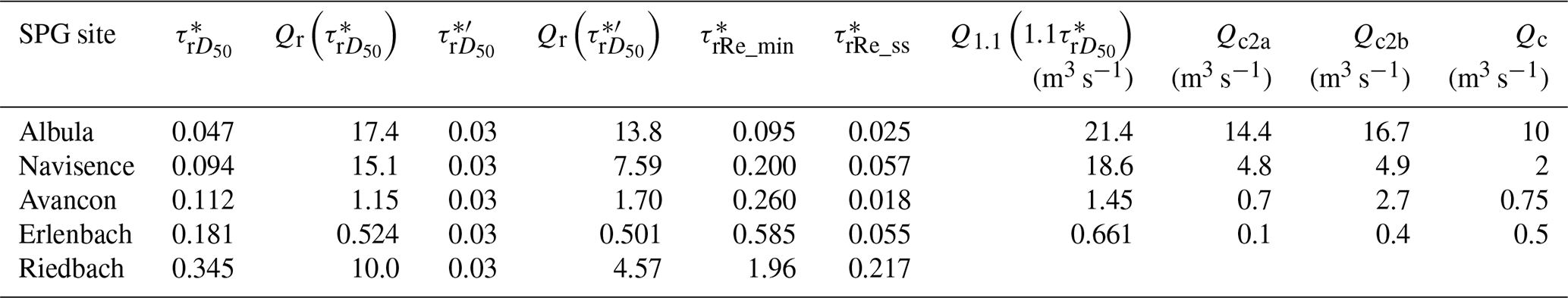
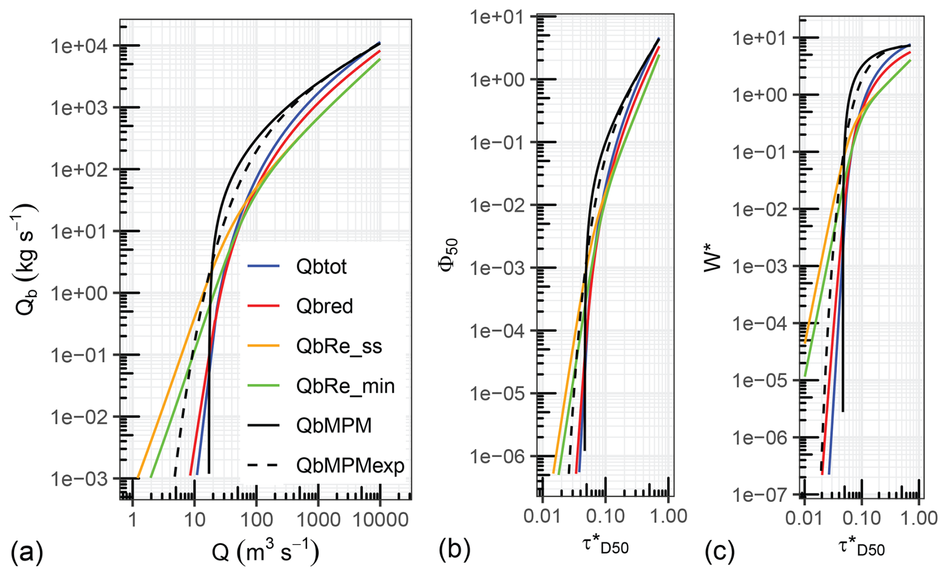
Figure 2 Bedload transport equations used and discussed in this study. To compare the six equations in one plot for each representation, they were applied here to the channel characteristics of the Albula River.

2.3 Determining the steepness of bedload relations and the reference shear stress based on observed transport rates for different time windows

Here I summarize the analysis to quantify the temporal variability of bedload transport during the active periods of bedload movement, which typically occurred in the summer half-year in the all the streams. For the Albula (2016), Navisence (2011), and Avançon (2019) streams I selected a year (given in parentheses) that included events with significant discharges and bedload transport rates. For the Erlenbach, I used the two main observation periods, A (1986–1999) and B (2002–2016). Each period included a similar total duration of active bedload movement as for the first three streams (Table 4).

Table 4 One-year-analysis of the temporal variations. Measured and calculated bedload masses for the Swiss streams and limiting discharges Q indicating phase-2-transport conditions. Bedload masses are given here for the entire observation period and for phase-2 flow periods only.

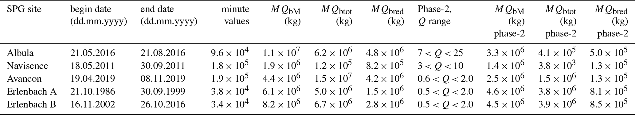
A closer inspection of the mean bedload transport relations over limited time periods, namely for two-week periods for the first three streams, showed that these relations varied over time within an intermediate flow range including phase-2 transport conditions. For each stream the phase-2 conditions suitable for this analysis were determined by visual inspection of the smoothened trend lines. There is not much quantitative guidance in the literature regarding the definition of phase-2 transport conditions. Bathurst (2007, Eqs. 8, 9, therein) proposed two empirical equations for the begin of phase-2 transport in mountain streams, Q_c2a as function of S and D₅₀, and Q_c2b as function of S and D₈₄, and I have included these two estimates in Table 3. A comparison with the values in Table 3 indicates, that some of these estimates approximately agree for two streams (Avancon, Q_c2a; Erlenbach, Q_c2b) with my values determined from the direct transport measurements.

For the Erlenbach stream, flow events involving bedload transport occurred sporadically, typically lasting only about 1–2 h. Therefore, I selected the characteristic sub-periods identified in Rickenmann (2024), namely 7 sub-periods for period A (1986–1999) and 6 sub-periods for period B (2002–2016). These sub-periods have similar disequilibrium ratios. This resulted in a roughly similar total number of minute values as for the two-week periods analyzed for the other three streams. The conditions of the analyzed discharge ranges for phase-2 transport conditions for the four streams are reported in Table 4, together with other summary information on bedload transport. This includes the total bedload mass summed over the summer half-year, for the observed yearly values MQ_bM, as well as for the calculated yearly values using the two SEA Eqs. (2) and (9), i.e. MQ_btot and MQ_bred.

Using the data for the phase-2 transport conditions only, I then determined power-law relations in the domain W^∗ vs. (${\mathit{\tau }}^{\ast }/{\mathit{\tau }}_{\mathrm{ref}}^{\ast }$) to approximate the measured bedload transport rates, resulting in one equation of the form of Eq. (12) for each two-week period (Albula, Navisence, and Avançon) or sub-period (Erlenbach). From the power-law relation fitted to the measurements, the exponent m is known, and by using the condition $W_{\mathrm{ref}}^{\ast }$ = 0.002 (Eq. 24), the dimensionless reference shear stress ${\mathit{\tau }}_{\mathrm{ref}}^{\ast }$ was determined according to Eq. (12). This procedure was applied with both SEA Eqs. (2) and (9), i.e. using $W_{\mathrm{tot}}^{\ast }$ and $W_{\mathrm{red}}^{\ast }$ separately for all investigated data sets. The variables determined from the $W_{\mathrm{tot}}^{\ast }$ analysis are labeled m_tot and ${\mathit{\tau }}_{D_{\mathrm{50}}}^{\ast }$, and those from the $W_{\mathrm{red}}^{\ast }$ analysis are labeled m_red and ${\mathit{\tau }}_{D_{\mathrm{50}}}^{\ast \prime }$.

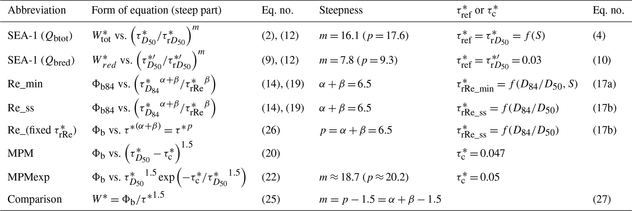
In the discussion section, I compare the exponents m obtained here for the Swiss streams with steepness of the Φ_b vs. τ^∗ relation of Recking et al. (2016), i.e. Eq. (19). In general, it can be shown that the two dimensionless bedload transport variables W^∗ and Φ_b are related to each other as:

$$\begin{array}{}\text{(25)}& W^{\ast }={\mathrm{\Phi }}_{\mathrm{b}}/{{\mathit{\tau }}^{\ast }}^{\mathrm{1.5}}\end{array}$$

For a given dimensionless reference shear stress, Eq. (19) can be simplified to:

$$\begin{array}{}\text{(26)}& {\mathrm{\Phi }}_{\mathrm{b}}=B{{\mathit{\tau }}^{\ast }}^{(\mathit{\alpha }+\mathit{\beta })}={{\mathit{\tau }}^{\ast }}^p,\end{array}$$

where B is a coefficient, $p=\mathit{\alpha }+\mathit{\beta }$, and the reference grain size for Φ_b may be D₈₄ or D₅₀. Comparing Eqs. (12), (25) and (26), the exponents can be related as follows:

$$\begin{array}{}\text{(27)}& m=\mathit{\alpha }+\mathit{\beta }-\mathrm{1.5}=p-\mathrm{1.5}\end{array}$$

For the case of α = 2.5 and β = 4 (Recking, 2012, 2013), this gives $m=\mathit{\beta }+\mathrm{1}=\mathrm{5}$, and $p=m+\mathrm{1.5}=\mathit{\alpha }+\mathit{\beta }+\mathrm{1.5}=\mathrm{6.5}$. A summary of the bedload transport equations is given in Table B1 in Appendix B.

2.4 Determining annual ratios of calculated to observed bedload masses based on observations for several years

If the analysis in Sect. 2.3 can be related to medium time scales, involving durations of about 5000 to 20 000 min for each time window, the following analysis attempts to quantify the variability of annual bedload masses. The basis for this analysis were extended datasets for the same four Swiss streams with typical observation durations of several years (Baldig and Rickenmann, 2024). The duration of active bedload transport for each year ranged from approximately 30 000–220 000 min and was therefore clearly longer than the time windows investigated in Sect. 2.3. In this part, I essentially determined two ratios to quantify the year-to-year variability in a given stream and to compare these ratios between the four sites. The first ratio was defined as follows:

$$\begin{array}{}\text{(28a)}& {\displaystyle }{r}_{x\mathit{\_}\mathrm{year}}=M{Q}_{\mathrm{btot}}/M{Q}_{\mathrm{bM}}\text{(28b)}& {\displaystyle }{r}_{x\mathit{\_}\mathrm{year}}=M{Q}_{\mathrm{bred}}/M{Q}_{\mathrm{bM}},\end{array}$$

which represents the yearly calculated (MQ_btot, MQ_bred) divided by the observed (MQ_bM) bedload mass. In the index, x = “tot” or x = “red”, according to the calculation with Q_btot or with Q_bred. The second ratio was defined as follows:

$$\begin{array}{}\text{(29a)}& {\displaystyle }\begin{array}{rl}{r}_{x\mathit{\_}\mathrm{inc}Q}=& \mathrm{slope}\mathrm{of}\mathrm{linear}\mathrm{model}\mathrm{between}\\ & \mathrm{Cumsum}\left(Q_{\mathrm{btot}}\right)\mathrm{and}\mathrm{Cumsum}\left(Q_{\mathrm{bM}}\right)\end{array}\text{(29b)}& {\displaystyle }\begin{array}{rl}{r}_{x\mathit{\_}\mathrm{inc}Q}=& \mathrm{slope}\mathrm{of}\mathrm{linear}\mathrm{model}\mathrm{between}\\ & \mathrm{Cumsum}\left(Q_{\mathrm{bred}}\right)\mathrm{and}\mathrm{Cumsum}\left(Q_{\mathrm{bM}}\right),\end{array}\end{array}$$

where the index “incQ” refers to the fact that here the yearly data was first ordered according to increasing Q values. Then a linear model was fitted to only those values for which ${\mathit{\tau }}_{D_{\mathrm{50}}}^{\ast }$ = > 1.1 ${\mathit{\tau }}_{\mathrm{r}{D}_{\mathrm{50}}}^{\ast }$ (for Eq. 29a) or for which ${\mathit{\tau }}_{D_{\mathrm{50}}}^{\ast \prime }$ = > 1.1 ${\mathit{\tau }}_{\mathrm{r}{D}_{\mathrm{50}}}^{\ast \prime }$ (for Eq. 29b). The reason for fitting the model only to values with larger flow intensities is motivated by the following arguments: (i) for larger flows, different bedload transport equations tend to predict more similar values (see e.g. Fig. 2), and (ii) the ratio of the dimensionless bankfull shear stress to the dimensionless reference shear stress is approximately in the range 1.16 ${\mathit{\tau }}_{\mathrm{r}{D}_{\mathrm{50}}}^{\ast }$ to 1.27 ${\mathit{\tau }}_{\mathrm{r}{D}_{\mathrm{50}}}^{\ast }$, and at bankfull flow considerable bedload transport may occur (Phillips and Jerolmack, 2019). Furthermore, I determined the ratio of calculated to observed bedload mass in chronological plots with cumulative sum values of Cumsum (Q_bx) $/$ Cumsum (Q_bM) as follows:

$$\begin{array}{}\text{(30a)}& {\displaystyle }{r}_{x\mathit{\_}\mathrm{chron}}=\mathrm{Cumsum}\left(Q_{\mathrm{btot}}\right)\mathrm{and}\mathrm{Cumsum}\left(Q_{\mathrm{bM}}\right)\text{(30b)}& {\displaystyle }{r}_{x\mathit{\_}\mathrm{chron}}=\mathrm{Cumsum}\left(Q_{\mathrm{bred}}\right)\mathrm{and}\mathrm{Cumsum}\left(Q_{\mathrm{bM}}\right)\end{array}$$

From these plots I determined a time duration for each year with begin of transport in spring, after which the ratio r_{x_chron} was approximately within a factor of three above or below the value r_{x_incQ}:

$$\begin{array}{}\text{(31)}& \mathrm{0.33}{r}_{x\mathit{\_}\mathrm{inc}Q}<r_{x\mathit{\_}\mathrm{chron}}<\mathrm{3}{r}_{x\mathit{\_}\mathrm{inc}Q}\end{array}$$

Note that the ratios r_{t_year} and r_{r_year} (Eq. 28) are equivalent with the values r_{t_incQ} and r_{r_incQ} (Eq. 29), respectively, at the end of a year.

3 Results

3.1 Comparison of observed bedload transport rates with predictive equations and mean annual trends for several years of observations

The bedload transport measurements at the five Swiss SPG-sites in Table 1 are compared in Fig. 3 to four different bedload transport equations described in chapter 2 and summarized in Table B1 (Appendix B). The four bedload transport equations applied in Fig. 3 are from Schneider et al. (2015a), namely SEA-1 (Q_btot, Eq. 5) and SEA-2 (Q_bred, Eq. 11), and the equation of Recking et al. (2016) for β = 4 (Eq. 14) using two different estimates of the reference shear stress, namely ${\mathit{\tau }}_{\mathrm{rRe}\mathit{\_}min}^{\ast }$ (Eqs. 17a, 18a, Q_{bRe_min}) and ${\mathit{\tau }}_{\mathrm{rRe}\mathit{\_}\mathrm{ss}}^{\ast }$ (Eqs. 17b, 18b, Q_{bRe_ss}). Summary values characterizing the annual bedload transport for four streams and for the selected year are given in Table 4.

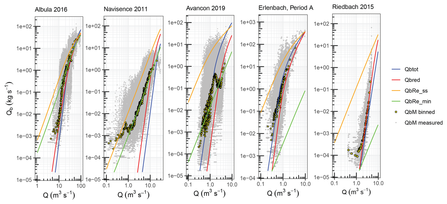
Figure 3 Comparison of bedload transport measurements (Q_b) at five Swiss streams with bedload transport calculations using for different predictive equations, shown as a function of discharge (Q). Erlenbach Period A refers to the years 1986–1999.

The first observation in Fig. 3 is a larger variability of measured Q_b values for a given discharge for the Navisence and the Avançon sites than for the other three sites. For the sites of Albula, Erlenbach (Period A), and Riedbach, the Q_b vs. Q data are more compact, and the mean trend, as determined by the geometric mean of the Q_b values for binned Q values, follows the steepness defined by the two SEA equations quite closely (with m_tot = 16.1 and m_red = 7.8). A caveat for the Riedbach data in Fig. 3 is that IMP values were stored only for 10 min intervals, with a corresponding temporal aggregation of the transport rates, a likely reason for less variability than in the other four streams. For the Navisence, the mean observed trend follows the steepness defined by the Recking equation with β = 4 (which is equivalent to m = 5.0, see Eq. 18) rather well. However, if further years or periods with SPG observations at the same sites are considered (similar plots for all available years are given in the Supplement), the picture may change: For the Albula (Figs. S1, S2, S3 in the Supplement), the mean trend for the steepness agrees better with the Recking equation with β = 4 for the years 2017 and 2020; it generally agrees better with the SEA equations for the year 2019; it has an intermediate steepness for the year 2018; and for the year 2021, the steepness is even lower than for the Recking equation with β = 4. For the Navisence (Figs. S12, S13), the mean observed trend aligns better with the SEA equations for 4 years (2013, 2019, 2020, 2021); for the year 2012, however, the mean observed steepness is intermediate between the two types of equations. For the Avançon (Figs. S20, S21) the result is mixed. Three years align better with the SEA equations (2018, 2019, 2023) and three years align better with the Recking equation (2020, 2021, 2022). Finally, for the period B at the Erlenbach, the observed steepness is somewhat intermediate between the two types of equations (Fig. S28). In conclusion, the mean (annual) bedload rating curves are rather variable from year to year, and unsurprisingly, differ between sites.

3.2 Temporal variability of steepness of the bedload relation and of the reference shear stress for phase-2 transport conditions

The identified phase-2 transport conditions for the four Swiss streams analyzed in this part are given in Table 4. An illustration of the temporal variation of the bedload transport over the entire discharge range is shown in Fig. 4 (no such analysis was made for the Riedbach, due to the limited time resolution of the measured Q_b values and the relatively narrow Q_b vs. Q relation in Fig. 3). In Fig. 4, the distinction of mean trends for the Q_b vs. Q relations for phase-2 transport conditions between different double-weeks or sub-periods is rather clear for the Albula, the Navisence, and the Erlenbach (for both periods A and B). However, the mean trends are less well defined for the Avançon. The more well-defined patterns of the temporally smoothened data in Fig. 4 for the Albula and the Erlenbach likely reflects the generally smaller variability of Q_b values in Fig. 3, as compared to the other two streams. Generally, the trends in the steepness of these relations for the two-week periods are similar to the trends defined by geometric mean values over the entire year shown in Fig. 3.

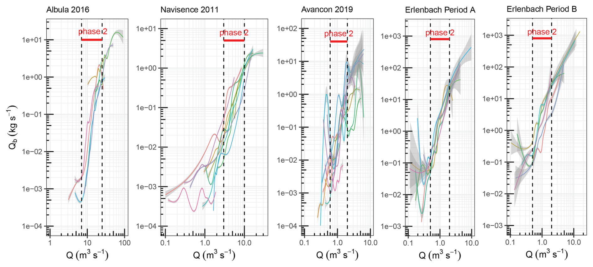
Figure 4 Temporal variability of bedload transport relations. The colored lines refer to the following time windows: for the Albula 7 consecutive double-week periods in summer 2016, for the Navisence 10 consecutive double-week periods in summer 2011, for the Avançon with 13 consecutive double-week periods in summer 2019, for the Erlenbach 7 sub-periods in period A (1986–1999) and 6 sub-periods in period B (2002–2016). The characteristic sub-periods for the Erlenbach were determined in Rickenmann (2024). The trend lines were determined by a loess smoothening function, a local polynomial regression fitting, in the R code. The two black dashed lines and the red arrow denote the phase-2 transport conditions, which were used in the analysis described in Sect. 2.3.

Table 5 Mean values of exponents m_tot, m_red and of dimensionless reference shear stresses ${\mathit{\tau }}_{\mathrm{r}{D}_{\mathrm{50}}}^{\ast }$, ${\mathit{\tau }}_{\mathrm{r}{D}_{\mathrm{50}}}^{\ast \prime }$ derived from analysis of temporal variation of bedload transport relation for phase-2 transport conditions. A full list with all the individual values for each stream is given in the Supplement (Table S1). For comparison, mean values of the variables from a similar analysis in Schneider et al. (2015a) for date sets “SEA_SS” and “SEA_HS” are also given here.

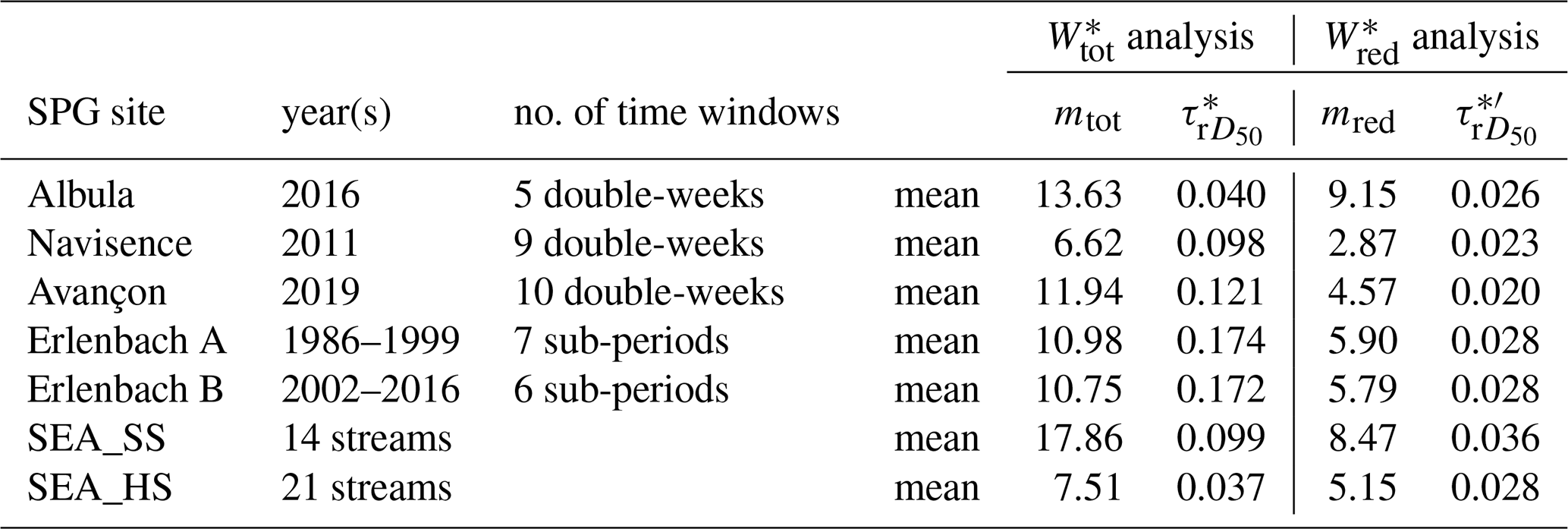
The quantitative results regarding the determined values of the exponents m and the dimensionless reference shear stresses ${\mathit{\tau }}_{\mathrm{ref}}^{\ast }$ are summarized in Table 5. The time-windows used to determine the trend lines (double weeks, sub-periods) involved durations of about 5000 to 20 000 min. The Supplement provides a full list of all the individual values for each stream (Table S1). In this quantitative analysis, not all time-windows (double week periods) shown in Fig. 4 yielded plausible results. This concerns the following number of excluded double week periods: 2 (out of 7) for the Albula, 1 (out of 10) for the Navisence, and 3 (out of 13) for the Avançon. All 13 sub-periods were used for the Erlenbach.

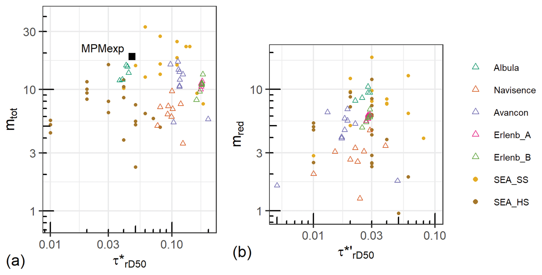
Figure 5 Variability of (a) m_tot vs. the ${\mathit{\tau }}_{\mathrm{r}{D}_{\mathrm{50}}}^{\ast }$ from $W_{\mathrm{tot}}^{\ast }$ analysis, and of (b) m_red vs. the ${\mathit{\tau }}_{\mathrm{r}{D}_{\mathrm{50}}}^{\ast \prime }$ from $W_{\mathrm{red}}^{\ast }$ analysis. The legend is the same for both plots.

A graphical illustration of the variability of m and ${\mathit{\tau }}_{\mathrm{ref}}^{\ast }$ is presented in Fig. 5a for the $W_{\mathrm{tot}}^{\ast }$ analysis, and in Fig. 5b for the $W_{\mathrm{red}}^{\ast }$ analysis. Datasets from Schneider et al. (2015a), namely SEA_SS and SEA_HS, are also included in both figures. Note that a similar analysis as described in Sect. 2.3 was performed in Schneider et al. (2015a) to determine values of m and ${\mathit{\tau }}_{\mathrm{ref}}^{\ast }$ for these latter data sets. Regarding the $W_{\mathrm{tot}}^{\ast }$ analysis, the mean m_tot values of the four Swiss streams generally fall between those of the SEA_SS and SEA_HS data sets (Table 5). The variability of the m_tot values for all the four Swiss streams (including temporal at-a-site and between-site variability) is in a similar range as for the SEA_SS and SEA_HS data sets (Fig. 5a). In general, the distribution of m and ${\mathit{\tau }}_{\mathrm{ref}}^{\ast }$ for the Swiss streams is more similar to that for the SEA_SS data (and also variable), whereas the SEA_HS data plot somewhat separately (Fig. 5a). The ${\mathit{\tau }}_{\mathrm{r}{D}_{\mathrm{50}}}^{\ast }$ values show a dependence for all the three data sets on channel slope (Fig. 6).

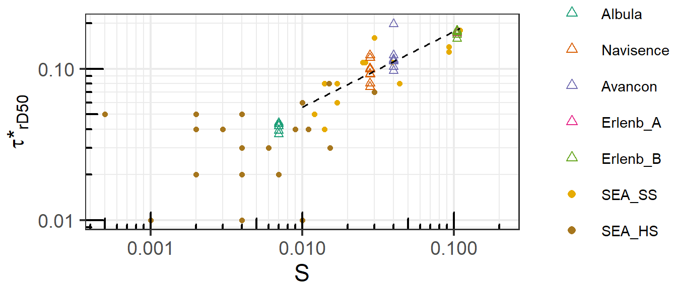
Figure 6 Variability of ${\mathit{\tau }}_{\mathrm{r}{D}_{\mathrm{50}}}^{\ast }$ (from $W_{\mathrm{tot}}^{\ast }$ analysis) with channel slope. The dashed black line represents Eq. (4), from a similar analysis in Schneider et al. (2015a).

Turning to the $W_{\mathrm{red}}^{\ast }$ analysis, the mean m_red values of the four Swiss streams fall again between those of the SEA_SS and SEA_HS data sets (Table 5). In general, the distribution of m and ${\mathit{\tau }}_{\mathrm{ref}}^{\ast \prime }$ for the Swiss streams is more similar to that for the SEA_HS data, whereas the SEA_SS data plot somewhat separately (Fig. 5b). The mean ${\mathit{\tau }}_{\mathrm{r}{D}_{\mathrm{50}}}^{\ast \prime }$ values for each of the four Swiss streams and for the SEA_SS and SEA_HS data sets range from 0.02 (Avançon) to 0.036 (SEA_SS) (Table 5). This is a typical range for Shield stresses or for ${\mathit{\tau }}_{\mathrm{ref}}^{\ast }$ values for bedload transport equations based on a reduced or effective shear stress, with again a similar variability for each of the three data sets.

3.3 Variability of annual ratios of calculated to observed bedload masses determined for several years of observations

Annual ratios of calculated to observed bedload masses were determined based on observations over several years. For a given year this analysis was based on total durations with bedload transport, which ranged from about 30 000 to 150 000 min (only two years for the Navisence include longer durations). The main quantitative results of this analysis are summarized for all four Swiss streams in Appendix C including Table C1, while some additional information is given separately for each stream in the Supplement (Tables S2, S3, S4, S5). The results of the analysis reported in Appendix C allowed to derive the approximate duration from the beginning of the transport season to the time point after which the r_{x_chron} values were within about a factor of 3 above or below the r_{x_incQ} values, x = t or r. Although there is quite some variability from year to year, the average relative duration, in terms of a fraction of the total transport duration of a year, was as follows (first number refers to the x = t and the second number to the x = r analysis): 51 % and 44 % for the Albula, 48 % and 39 % for the Navisence, 15 % and 21 % for the Avançon, and 6 % and 11 % for the Erlenbach (Table C1).

A similar picture becomes apparent when comparing the ratios r_{t_year} and r_{r_year} (Fig. 7a) and the ratios r_{t_incQ} and r_{r_incQ} (Fig. 7b) for the four streams, for both the $W_{\mathrm{tot}}^{\ast }$ analysis and for the $W_{\mathrm{red}}^{\ast }$ analyses: While there is a tendency to under-estimate the observed bedload masses for two streams (Albula, Erlenbach), a tendency for an over-estimation is apparent for the other two streams (Navisence, Avançon). The variability of the ratios for a given stream and type of analysis ($W_{\mathrm{tot}}^{\ast }$ or $W_{\mathrm{red}}^{\ast }$) is similar for all cases. The effect of flow or transport intensity on the ratios r_{t_year} (Fig. 8a) and r_{r_year} (Fig. 8b) was considered by plotting these ratios against $Q_{max}/Q_{\mathrm{1.1}}$, where Q_max is the maximum water discharge for a given year and Q_1.1 is the water discharge corresponding to a dimensionless shear stress${\mathit{\tau }}_{D_{\mathrm{50}}}^{\ast }$ = 1.1 ${\mathit{\tau }}_{\mathrm{r}{D}_{\mathrm{50}}}^{\ast }$ (Table 3). For the Albula, the ratios indicate that the calculated and observed bedload masses are more closely aligned at higher flow intensities. For the other three streams, no clear trend appears. However, when accounting for all the stream sites, one may see a slight trend towards increased agreement between the calculated and observed bedload masses for increasing flow intensities This is somewhat clearer for the $W_{\mathrm{red}}^{\ast }$ analysis than for the $W_{\mathrm{tot}}^{\ast }$ analysis.

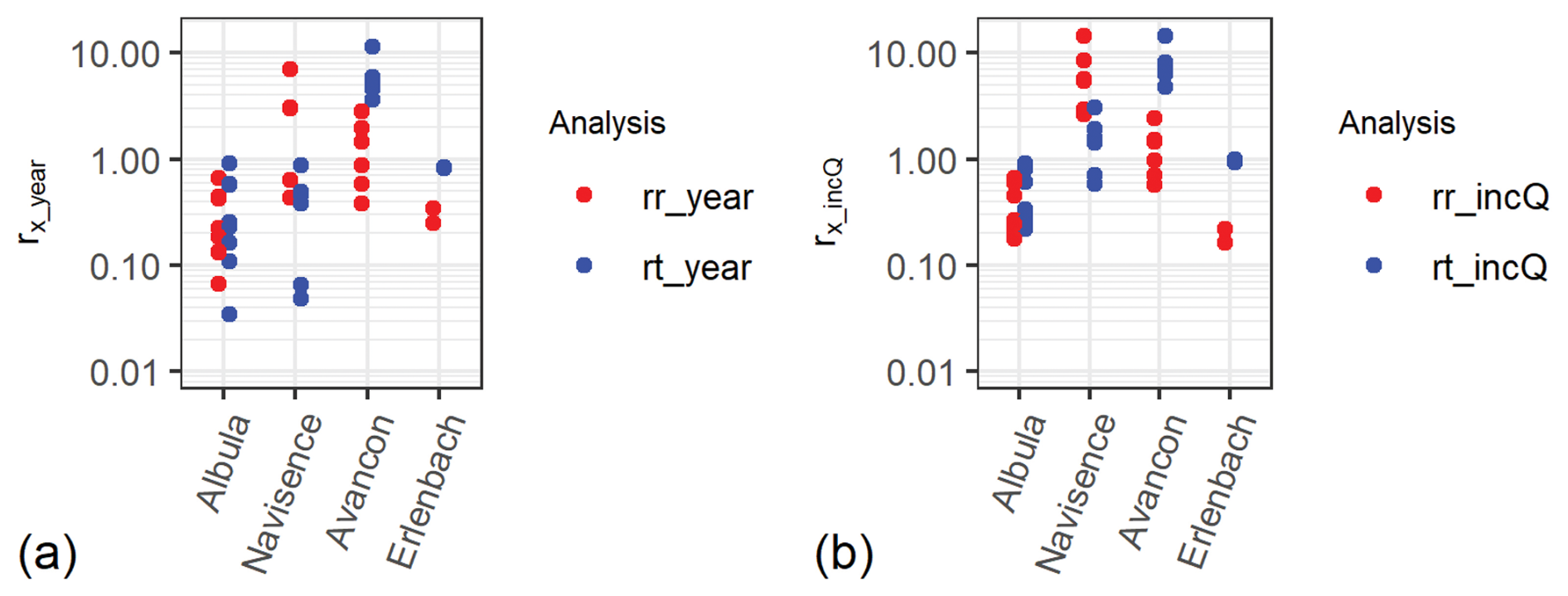
Figure 7 Variability of (a) r_{x_year} and (b) r_{x_incQ}, separately for the analysis with the Q_btot calculations (x=t) and for the Q_bred calculations (x=r).

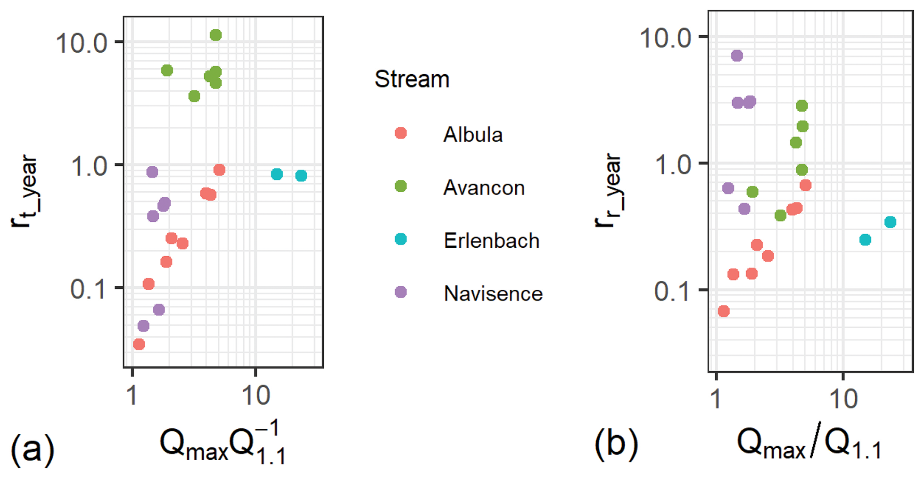
Figure 8 Variability of (a) r_{t_year} and (b) r_{r_year}, plotted against normalized maximum discharge ($Q_{max}/Q_{\mathrm{1.1}}$) in each year.

For a given stream with several years of observations, the 15 mean values of the four ratios r_{t_year}, r_{r_year}, r_{t_incQ}, and r_{r_incQ} typically vary in a range of about 0.3 to 3, with two smaller r values (r_{r_year} for the Albula, r_{r_incQ} for the Erlenbach) and with two larger r values (r_{t_year} for the Avançon, r_{r_incQ} for the Navisence) (Table C1). Thus, considering a time-period of several years, the mean annual ratios of predicted to measured bedload masses are roughly within a factor of 3 above and below a perfect agreement.

4 Discussion

4.1 General comments on the bedload transport equations

The MPM equation has often been applied in studies on gravel-bed rivers, and it is implemented in many numerical software codes to simulate bedload transport, typically for longer river reaches in 1D or also in also in selected river reaches in 2D simulations. Such software tools include HEC-RAS (Yavuz, 2025), Telemac (Villaret et al., 2013) and Basement (Vanzo et al., 2021). As can be seen in Fig. 2, the original MPM equation has an important drawback, in that the predicted transport rates in the vicinity of the critical Shields number ${\mathit{\tau }}_{\mathrm{c}}^{\ast }$ almost encounter a step-function because the MPM relation (Eq. 20, hereafter referred to as original MPM) approaches a vertical line for dimensionless shear stresses slightly larger than but approaching the ${\mathit{\tau }}_{\mathrm{c}}^{\ast }$ value. Therefore, it is much more sensitive in this shear stress range to the choice of the characteristic grain size D₅₀, which is typically needed to estimate an appropriate ${\mathit{\tau }}_{\mathrm{c}}^{\ast }$ or ${\mathit{\tau }}_{\mathrm{ref}}^{\ast }$ value, than the other equations. Four of the other predictive equations in Fig. 2 use a dimensionless reference shear stress, and the exponential form of the MPM equation (Eq. 22, hereafter referred to as MPMexp) results in a bedload transport relation that is qualitatively more similar to the SEA and the Recking equations than to the original MPM equation. For comparison, the mean steepness of Eq. (22) in Fig. 2c was calculated for bedload transport intensities in the range 1 × 10⁻⁷ < W^∗ < 0.002 (the larger value corresponding to a dimensionless reference shear stress = 0.047) by approximating a power law, and this gives an equivalent exponent of m = 18.7. This value is rather close to the characteristic values for the SEA_SS data set, with a mean m = 17.9 (Table S1) and a median m = 16.1 which is used in Eq. (2a) to calculate $W_{\mathrm{tot}}^{\ast }$ or Q_btot. The value of m = 18.7 for ${\mathit{\tau }}_{\mathrm{ref}}^{\ast }$ = 0.047 for the MPMexp equation in the given range of W^∗ values is included in Fig. 5 for comparison; this data point is positioned at the outer perimeter of the CH_TV and the SEA_SS data.

If the Recking equations (Eqs. 19, 18a, 18b) are presented in the W^∗ vs. ${\mathit{\tau }}_{D_{\mathrm{50}}}^{\ast }$ (or ${\mathit{\tau }}_{D_{\mathrm{84}}}^{\ast }$) form, the exponent (steepness) is m = 5 (Fig. 2, Eq. 27). Thus, they define flatter bedload transport relations for small to medium flow intensities than the SEA Eqs. (2) and (9), and for the three Swiss streams with channel slopes smaller than 5 % (Albula, Navisence, and Avançon) they tend to predict larger transport rates than the latter (Figs. 2, 3). In the Φ_b vs. ${\mathit{\tau }}_{D_{\mathrm{50}}}^{\ast }$ (or ${\mathit{\tau }}_{D_{\mathrm{84}}}^{\ast }$) representation, the exponent p for the steep part is (Eq. 26) p = 6.5 for the Recking Eq. (19), and p = 17.6 for the SEA-1 Eq. (2a) and p = 9.3 for the SEA-2 Eq. (9a). Thus, the steepness of the SEA-equations is considerably larger than those of Eqs. (14), (19), (26) with α = 2.5 and β = 4. The range of steepness values for the two types of equations, when adapted to measured bedload transport rates, is discussed in the following discussion section.

In the study of Schneider et al. (2015a) both the equations SEA-1 and SEA-2 (Fig. 2, equations for Q_btot and Q_bred) and the original Wilcock and Crowe (2003) equation were compared to field data from a total of 35 mountain streams and gravel-bed rivers (SEA_SS and SEA_HS data sets). The original Wilcock and Crowe (2003) equation is based on flume experiments representing transport-limited conditions. Yet this equation is not too dissimilar to the SEA-1 and SEA-2 equation, and all the three equations approximately represent a mean trend of the field data of the 35 streams, which show a variability in transport levels of three to four orders of magnitude for a given Shields stress (Schneider et al., 2015a, Fig. 7 therein). Thus, it cannot be claimed that the flume-based bedload transport equation SEA-1 and SEA-2 truly represent transport-limited conditions.

4.2 Comparison of the steepness and the dimensionless reference shear stress with the REA study

In this section, I compare the range of values obtained by analyzing the temporal variation of the bedload relations for phase-2 transport in the four Swiss streams (Sect. 3.2) with the results reported in Recking et al. (2016; “REA study”). Henceforth the data set of the four Swiss streams for the analysis of m and ${\mathit{\tau }}_{\mathrm{ref}}^{\ast }$ (as included in Figs. 5 and 6; Sect. 3.2) is labeled “CH_TV” (TV for temporal variation), and the data set of Recking et al. (2016) is labeled “REA_BT” (BT for β and ${\mathit{\tau }}_{\mathrm{ref}}^{\ast }$) henceforth; these labels are used in Figs. 9, 10, and 11.

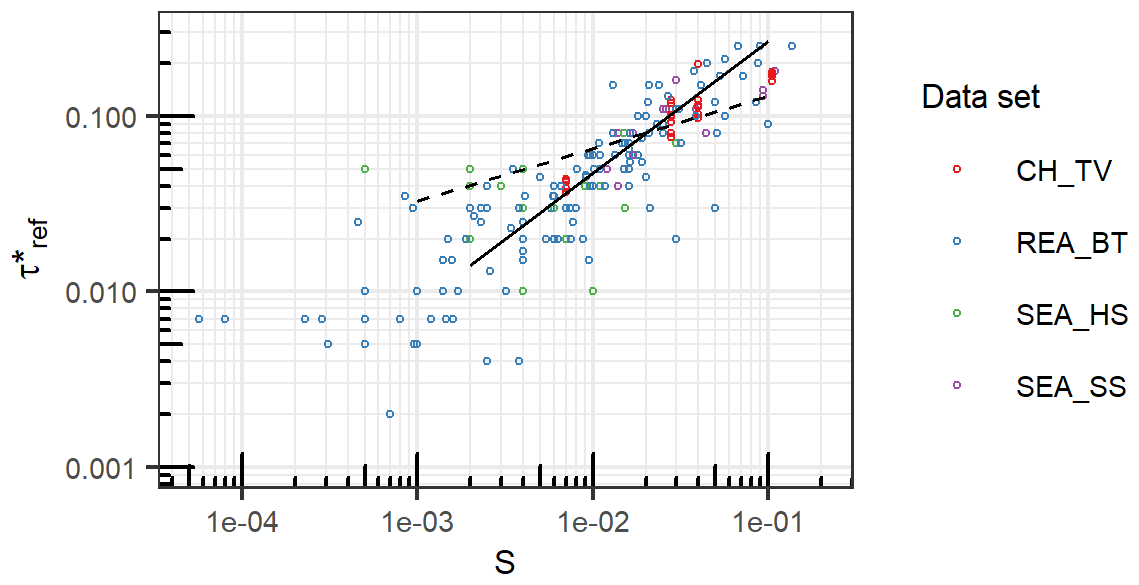
Figure 9 Optimized values of ${\mathit{\tau }}_{\mathrm{ref}}^{\ast }$ vs. channel slope S, for various datasets. For the CH-TV, SEA_SS and SEA_HS data, ${\mathit{\tau }}_{\mathrm{ref}}^{\ast }$ was determined based on a $W_{\mathrm{tot}}^{\ast }$ analysis. For the REA_BT data, ${\mathit{\tau }}_{\mathrm{ref}}^{\ast }$ was derived from the Recking equation assuming a fixed exponent β = 4 (case 1 analysis). The solid black line is Eq. (33) derived from the REA_BT data with a plane-bed morphology. The dashed black line is Eq. (32) from Recking et al. (2016) based on flume experiments and used in their case-2 analysis.

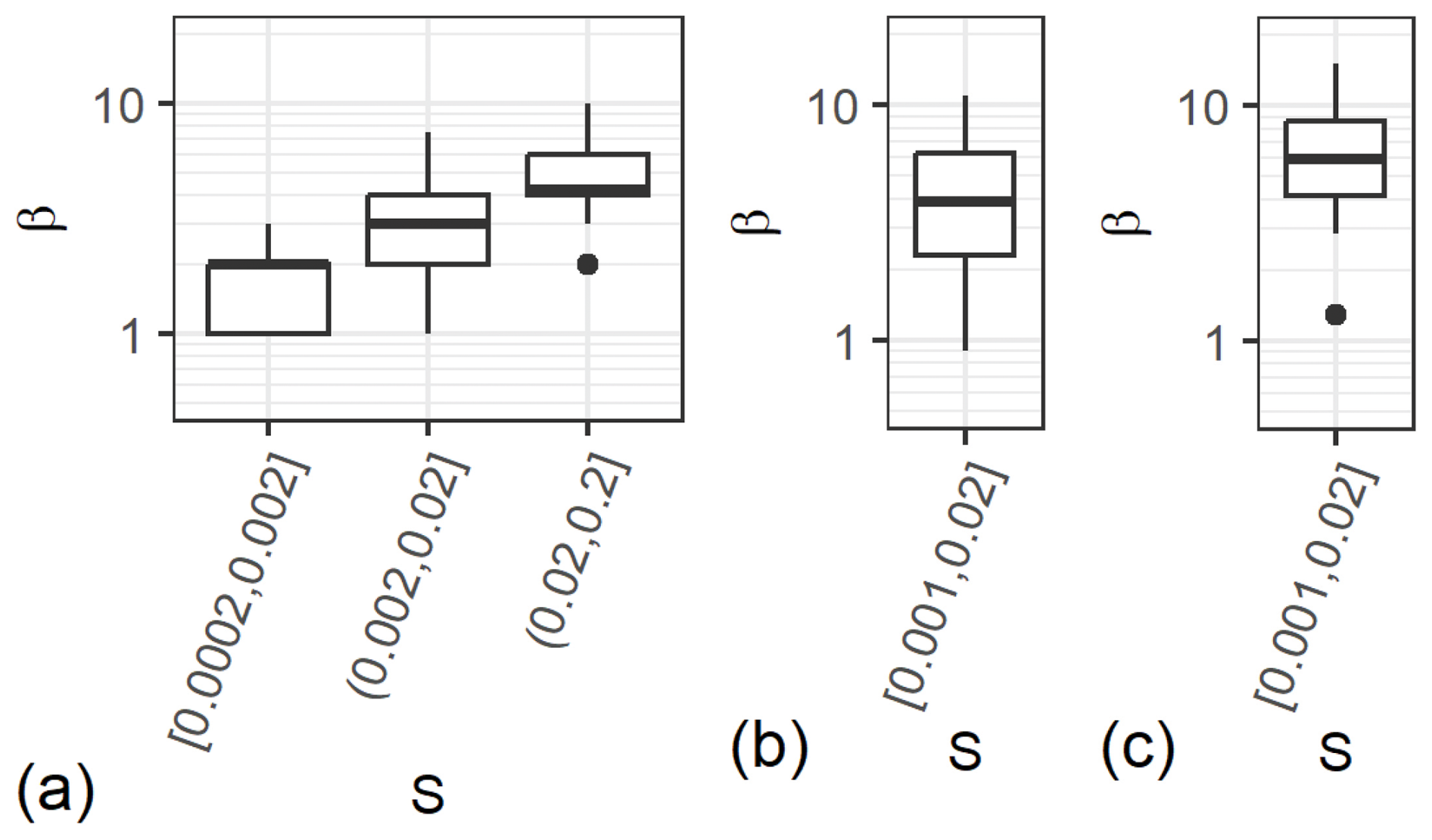
Figure 10 Boxplots of the exponent β for different for channel slope classes. (a) for the entire REA_BT data, for the case 2 analysis assuming Eq. (23) to pre-define the ${\mathit{\tau }}_{\mathrm{ref}}^{\ast }$ values, (b) for the SEA_HS data, derived from the $W_{\mathrm{red}}^{\ast }$ analysis, (c) for the SEA_HS data, derived from the $W_{\mathrm{tot}}^{\ast }$ t analysis. For the SEA_HS data from Schneider et al. (2015a), 19 out of 21 data points fall into the slope class shown here.

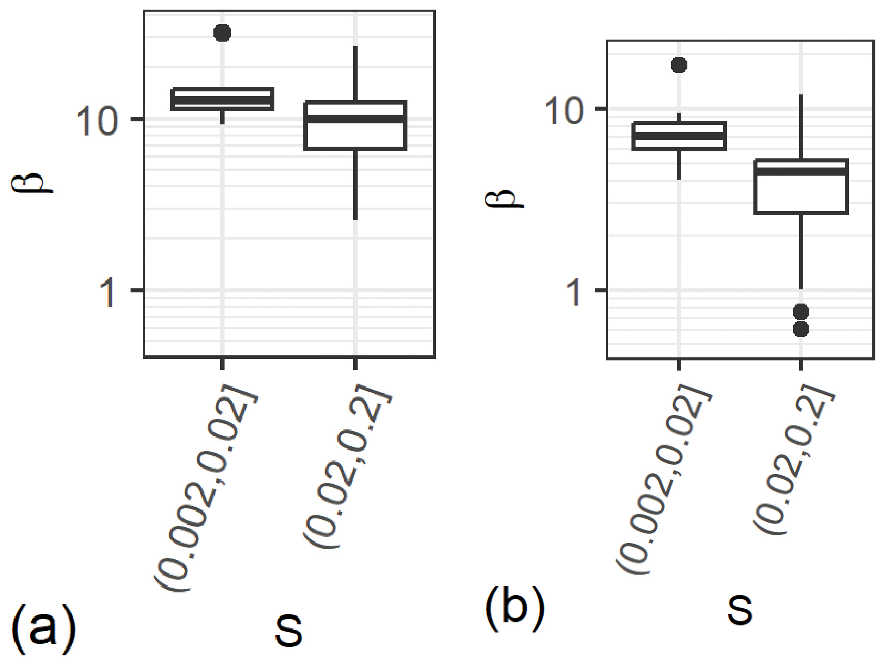
Figure 11 Boxplots of β for the CH_TV and SEA_SS data combined, for 2 slope classes, derived (a) from the $W_{\mathrm{tot}}^{\ast }$ analysis, and (b) from the $W_{\mathrm{red}}^{\ast }$ analysis.

As a caveat it must be mentioned that Recking et al. (2016) varied either the exponent β (steepness) of Eqs. (14) and (19) or the reference shear stress ${\mathit{\tau }}_{\mathrm{refRe}}^{\ast }$, to find a good agreement of the predictions with the measurements, while the other variable was prescribed. Namely (case 1 analysis) they fixed β = 4 when optimizing the ${\mathit{\tau }}_{\mathrm{refRe}}^{\ast }$ values, or (case 2 analysis) when optimizing the β values they set ${\mathit{\tau }}_{\mathrm{refRe}}^{\ast }$ as a function of the channel slope as:

$$\begin{array}{}\text{(32)}& {\mathit{\tau }}_{\mathrm{refRe}}^{\ast }=\mathrm{0.26}{S}^{\mathrm{0.3}}\end{array}$$

which is based on flume experiments and should provide a better link of Eq. (14) with the bedload transport measurements in flume experiments. For the results obtained in this study for the four Swiss streams in Sect. 3.2, however, both the exponents m and the ${\mathit{\tau }}_{\mathrm{ref}}^{\ast }$ values were optimized in the same step (Sect. 2.3). For their case 1 analysis, Recking et al. (2016) found a strong dependence of the ${\mathit{\tau }}_{\mathrm{refRe}}^{\ast }$ values for plane beds on channel slope, approximated with a power law relation as:

$$\begin{array}{}\text{(33)}& {\mathit{\tau }}_{\mathrm{refRe}}^{\ast }=\mathrm{1.5}{S}^{\mathrm{0.75}}\end{array}$$

My results for the ${\mathit{\tau }}_{\mathrm{r}{D}_{\mathrm{50}}}^{\ast }$ values based on the $W_{\mathrm{tot}}^{\ast }$ analysis in Fig. 6 compare fairly well with the results of Recking et al. (2016) as illustrated in Fig. 9. The power law relation (Eq. 33) is quite similar to a relation found by Schneider et al. (2015a) for the SEA_HS data set using total shear stress (for which both the exponents m and the ${\mathit{\tau }}_{\mathrm{ref}}^{\ast }$ values were optimized). On the other hand, the relation obtained by Schneider et al. (2015a) for the SEA_SS data set using total shear stress (Eq. 2a), Eq. (4), lies between the two power law relations (32) and (33). However, for channel slopes in the range 0.01 < S < 0.1, the ${\mathit{\tau }}_{\mathrm{ref}}^{\ast }$ values predicted by Eqs. (32) and (33) are similar to those predicted by Eq. (4), as can also be seen by comparing Figs. 6 and 9. These results suggest that a comparison between the two approaches may be justified.

Turning now to the case 2 analysis of Recking et al. (2016), the range of their optimized β values depends to some extent on channel slope (Fig. 10a). This is in contradiction to the ranges of the β values from the CH_TV and the SEA_SS data set together (converted from m values with Eq. 27) (Fig. 11), for which only the β values for the largest slope class (0.02, 0.2] from the $W_{\mathrm{red}}^{\ast }$ analysis approximately agree with the β values of Recking et al. (2016) for the same slope class. If we consider only the SEA_HS data, the β values from the $W_{\mathrm{red}}^{\ast }$ analysis (Fig. 10b) agree better with the β values of Recking et al. (2016) for the same slope class (Fig. 10a) than the β values from the $W_{\mathrm{tot}}^{\ast }$ analysis (Fig. 10c).

4.3 Possible implications of the above comparison and some limitations

In summary, the results of the case 1 analysis of Recking et al. (2016) regarding the ${\mathit{\tau }}_{\mathrm{ref}}^{\ast }$ values are roughly in better agreement with the $W_{\mathrm{tot}}^{\ast }$ analysis of the Swiss streams and the SEA_SS data. Conversely, the results of their case 2 analysis regarding the β or m values are roughly in better agreement with the $W_{\mathrm{red}}^{\ast }$ analysis of the Swiss streams and the SEA_HS data. This suggests that the bedload transport equation of Recking et al. (2016), using D₈₄ for the definition of Φ_b84 and of ${\mathit{\tau }}_{D_{\mathrm{84}}}^{\ast }$, is an approach somewhere intermediate between the bedload transport equations SEA-1 ($W_{\mathrm{tot}}^{\ast }$) and SEA-2 ($W_{\mathrm{red}}^{\ast }$), using D₅₀ as a reference grain size. It is likely that the use of a slope-dependent ${\mathit{\tau }}_{\mathrm{ref}}^{\ast }$ value (Eq. 23) in the case 2 analysis resulted in a channel slope-dependence of the optimized β values (Fig. 10a): Eqs. (32, case 2) and (33, case 1) cross each other at about S = 0.02. For S > 0.2, ${\mathit{\tau }}_{\mathrm{ref}}^{\ast }$ (Eq. 32) is smaller than ${\mathit{\tau }}_{\mathrm{ref}}^{\ast }$ (Eq. 33) (Fig. 9) which has to be compensated by a value β > 4 (Fig. 10a) to result in a similar bedload transport level for the two analyzed cases; conversely, for S < 0.2, ${\mathit{\tau }}_{\mathrm{ref}}^{\ast }$ (Eq. 32) is larger than ${\mathit{\tau }}_{\mathrm{ref}}^{\ast }$ (Eq. 33; Fig. 9) which has to be compensated by a value β < 4 (Fig. 10a).

Recking et al. (2016, and their Fig. 9) argued that their approach (Eq. 14) using D₈₄ as a reference grain size is roughly equivalent to using a reduced or effective shear stress with D₅₀ as a reference grain size, by showing that for their data set ${\mathit{\tau }}_{D_{\mathrm{84}}}^{\ast }$ ≪ ${\mathit{\tau }}_{D_{\mathrm{50}}}^{\ast }$ and ${\mathit{\tau }}_{D_{\mathrm{84}}}^{\ast }$ ≈ ${\mathit{\tau }}_{D_{\mathrm{50}}}^{\ast \prime }$, where the latter values were determined with a similar approach as used for the SEA equations. For our data sets with the four Swiss streams, a similar comparison was made (Fig. S31), confirming a similar pattern for three sites (except for the Albula site, for which ${\mathit{\tau }}_{D_{\mathrm{84}}}^{\ast }$ ≪ ${\mathit{\tau }}_{D_{\mathrm{50}}}^{\ast \prime }$ was observed). The analysis above showed, however, that the results of Eq. (14) are not directly comparable with the results of the $W_{\mathrm{red}}^{\ast }$ equation (Eq. 9). Two other elements may also contribute to the fact that the approach of Eq. (14) generally requires smaller β or m values than Eq. (9), particularly for channel slopes smaller than about 0.02. First there is the problem that the Helley-Smith sampler applied in gravel bed streams tends to over-sample at low and to under-sample at higher transport intensities, resulting in a generally less steep bedload vs. discharge relation (Bunte and Abt, 2005; Bunte et al., 2008; Schneider et al., 2015a). The β values of the $W_{\mathrm{red}}^{\ast }$ analysis (Eq. 9) for the SEA_HS data are about in the range of 2 to 6 (Fig. 10b), and the β values of REA_BT data in the range of 2 to 4 for the same slope class (Fig. 10a); this slight difference may be associated with somewhat smaller ${\mathit{\tau }}_{D_{\mathrm{50}}}^{\ast \prime }$ values found for the SEA_HS data (Schneider et al., 2015a, Fig. 3b therein) than those pre-defined for the case 2 analysis using Eq. (32). Second, an inspection of the REA_BT dataset showed that for about half these streams a temporal variation of the measured bedload transport data could be identified (for 47 streams I could identify reliable time and date data, and the Q_b vs. Q data showed a time-dependence for 23 streams, no time-dependence for 18 streams, and the patterns was inconclusive for 6 streams); if such bedload transport data is averaged arithmetically it may lead to lower β or m values, because this neglects a lateral shift of the transport relation as observed for the four Swiss streams (Fig. 4).

The analysis of the beta exponents of Recking et al. (2016) showed that the steepness of the bedload relation is generally somewhat steeper and more variable in mountain streams, i.e. for plane bed and step-pool streams as compared to streams with a riffle-pool or braided morphology, than for wider streams with a flatter channel slope. A possible reason for this may be that more fine particles are available in flatter streams, leading to larger transport and generally lower β or m values according to the Recking Eq. (14). Recking et al. (2016) also found that for riffle-pool morphologies the grain-size distribution, likely a proxy for the riffle-pool development, influences the optimal reference shear stress. In general, both the Recking Eq. (14) and the two SEA Eqs. (2) and (9) are considered to provide a useful reference calculation framework for bedload transport levels, which can be used to quantify other influencing factors (apart from the hydraulic forcing), such as sediment supply or availability and bed morphology, that can help to further constrain the variables steepness (exponent) and reference shear stress in these approaches.

4.4 Annual ratios of calculated to observed bedload masses

In general, many bedload transport equations have an exponent p = 1.5 in a Φ_b vs. τ^∗ relation (Eq. 26) for large flow and transport intensities (including Eqs. 2, 9, 20, 22), and this implies that the bedload transport rate Q_b is approximately linearly related to discharge Q (see also Fig. 2a). This motivated the analysis outlined in Sect. 2.4 with the results presented in Sect. 3.3. Although there is still considerable variability of the annual ratios shown in Figs. 7 and 8, the four ratios r_{t_year}, r_{r_year}, r_{t_incQ}, and r_{r_incQ} typically vary in a range of about 0.33 to 3 for a given stream (Table C1), thus confirming the motivation for this analysis.

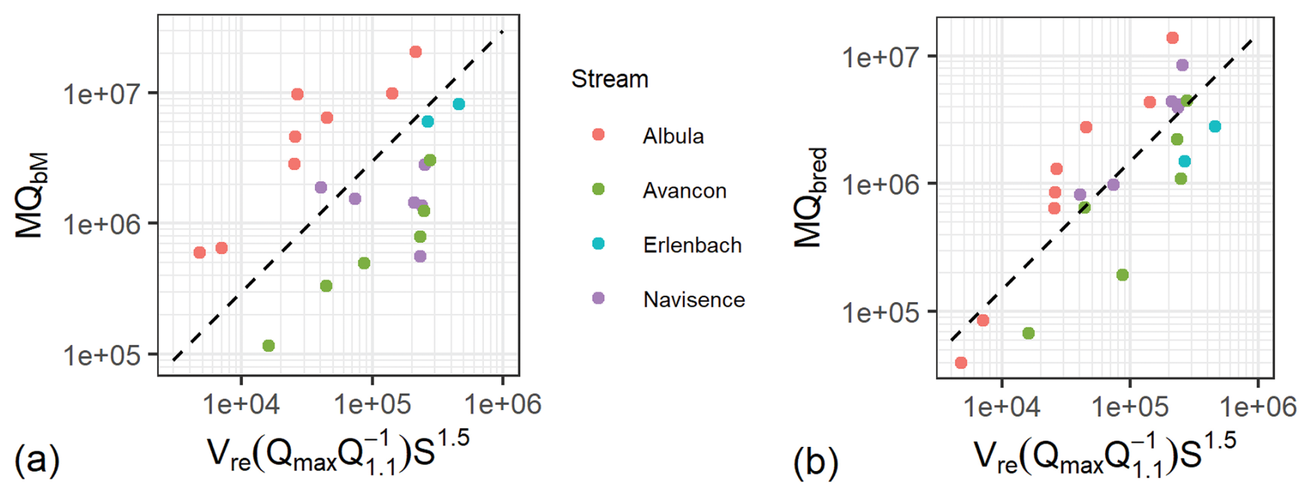
Figure 12 Yearly bedload masses vs. a simple measure of flow strength, as $V_{\mathrm{re}}(Q_{max}/Q_{\mathrm{1.1}})S^{\mathrm{1.5}}$. (a) The measured yearly bedload mass, sum (Q_bM), and (b) the calculated yearly bedload mass using Eq. (9), sum (Q_bred). The dashed black lines indicate a linear relation, the position of which was chosen to approximately fit the trend defined by the data of the four streams.

Evidence for such an approximately linear relation between yearly observed bedload masses and simple measures of flow intensity were already presented for the Erlenbach (Rickenmann, 1997; Rickenmann, 2020, Fig. S7 therein), and for the Albula and the two Austrian mountain streams Fischbach and Ruetz (Rickenmann, 2018; Rickenmann et al., 2020a). In Rickenmann (2018, Fig. S15 therein) it was shown that the ratio sum (Q_bM) $/$ sum (Q) converged to an agreement within a factor of 2 after about 50 to 60 d of transport for both Austrian streams. For the Erlenbach and the other two streams, the yearly sum (Q_bM) values also showed a correlation with the yearly excess runoff volume V_re = sum (Q−Q_c), multiplied by (the normalized) maximum discharge (Rickenmann, 1997; Rickenmann et al., 2020a). Q_c is a critical discharge above which more intense bedload transport starts. For the four Swiss streams of this study a similar analysis confirmed this earlier empirical finding of an approximately linear relation between either yearly observed bedload masses calculated with Eq. (9) or yearly measured bedload masses and a simple measure of the yearly flow intensity (Fig. 12). In this context it is of interest, that the analysis of several bedload-transporting flood events in Summer 2005 in Switzerland also confirmed the existence of such an approximately linear relation between observed bedload masses and simple measures of flow intensity, integrated over the flood event duration (Rickenmann and Koschni, 2010). Further independent evidence of a better agreement between calculated and measured bedload transport levels for higher or longer flow intensities is presented by Recking et al. (2012), who found a clearly increasing agreement between calculated and observed transport for either longer integration periods and/or relative flow intensities ${\mathit{\tau }}^{\ast }/{\mathit{\tau }}_{\mathrm{c}}^{\ast }$ larger than about 1.2.

4.5 Roles of variable sediment supply and of changing reference Shields stress

It is challenging to discuss possible reasons for changing sediment supply conditions (or sediment availability on the streambed) for the four Swiss streams, including multiple years of bedload transport measurements, because of limited additional observations available. For the Erlenbach, it had been found that extreme events with a high peak discharge likely caused the break-up of step structures and a destabilization of bank zones, resulting in more movable sediment stored on the streambed, a decrease in critical Shields stress, an increased bedload transport level over the following years and an increased range of variability (Rickenmann, 2020). Based on SPG measurements in the Austrian Drau River, Aigner et al. (2017) observed bedload pulses with increased bedload transport levels about one to two orders of magnitude larger than pre- or post-pulse transport levels. The pulses were triggered by flow events with moderate to high discharges and occurred in a reach with no sediment supply from tributaries. They concluded that the likely sediment source was located in the roughly 2 km long reach upstream of the SPG site and that bedload pulses resulted from an entrainment of stored riverbed or bank material once water discharge had exceeded a critical value, and that no armour layer break-up had occurred. Kreisler et al. (2017) examined bedload transport behaviour in the Austrian Urslau mountain stream for three years, also based on SPG measurements. They found elevated bedload transport levels in the first period for two observation years, at the time of the occurrence of higher discharges. During later periods in these two years, transport efficiencies decreased by about a factor of two to three on average, which they attributed to an exhaustion of sediment availability, and the bedload-transport variability extended up to two orders of magnitude for a given flow discharge. They presumed that the main sediment sources for the temporarily increased bedload transport in the Urslau stream were erosion processes in tributaries supplying sediment during the high-flow events.

The fact that bedload-transport variability may be due to a combination of changing sediment supply and grain size composition of the bed surface or of the transported material complicates a clear separation of these effects. For example, higher transport levels than defined by the transport equations (as applied in this study) may be due to predominantly finer transported material, that may be underpredicted because a fixed reference grain size D₅₀ was assumed for the predictions. On the contrary, lower transport levels than defined by the equations may be a result of either a sediment supply limitation or of a coarser D₅₀ than assumed for the predictions. The distinction of these two aspects is further complicated in the case of armoured beds when the D₅₀ of the transported material is (substantially) different from the D₅₀ of the bed surface. For example, Piton and Recking (2017) discussed observations from the Roize mountain stream in France, for which predictions of the annual bedload transport differed by about two orders of magnitude depending on the assumed characteristic grain size of the transported material (bed surface versus “traveling bedload”). Another example, illustrating the combined effect of changing sediment supply and changing D₅₀ of the bed surface is the flume study of Johnson et al. (2015) and Johnson (2016). Johnson performed experiments with initial channel slopes varying between 8 % and 12 %, with a constant flow discharge, and over a limited time period he fed sediment finer than the bulk of the bed material. For the feeding period he observed a reduction of the D₅₀ of the bed surface, a reduction of the dimensionless reference shear stress ${\mathit{\tau }}_{\mathrm{ref}}^{\ast }$, and a concomitant increase in bedload transport rates. He back-calculated the reference shear stress ${\mathit{\tau }}_{\mathrm{ref}}^{\ast }$ using the Wilcock and Crowe (2003) equation, and the values of ${\mathit{\tau }}_{\mathrm{ref}}^{\ast }$ varied in a similar range as those for the four Swiss streams illustrated in Fig. 5a.

Recking (2012) proposed to classify mountain streams into three categories of sediment supply, namely “high supply”, “moderate supply”, and “low supply”. This classification was based on introducing possible boundaries between the three categories in a graph of dimensionless bedload transport versus normalized bed shear stress. For each of the four Swiss study streams Albula, Navisence, Avançon, and Erlenbach, the numerous minute values of the bedload measurements of this study fall into all the three categories of sediment supply of Recking. On the contrary, the classification of Recking (2012) is based on only a limited number of measurements available per stream, which may have favoured a between-site differentiation. It may also be mentioned that the four study streams Navisence, Avançon, Erlenbach, and Riedbach represent pristine mountain streams, whereas the Albula is a larger mountain river with important hydropower installations upstream of the SPG measuring site. Nevertheless, the range of bedload-transport variability found for these study streams from the combined between-site and at-a-site comparison is generally comparable to the between-site variability associated with the REA_BT data set including a large number of stream sites.

4.6 Implications for bedload prediction and modelling

For the streams with channel slopes smaller than about 2 %, the Recking-study determined steepness values that are generally smaller than those found for the four Swiss streams and a data set in Schneider et al. (2015a) (Fig. 10b, c). Furthermore, for the case 2 analysis of Recking et al. (2016) there is a trend for flatter streams to have smaller steepness values β than for the steeper streams of their data set (Fig. 10a). It is hypothesized that the larger β values for flatter streams are possibly due to a higher availability of fine particles in these streams, in line with the general concept in fluvial geomorphology that relative sediment supply increases and relative transport capacity decreases with increasing catchment area (Montgomery and Buffington, 1997). Apart from this general trend, it is difficult to provide more and clear guidance on the choice of a suitable transport equation, based on the analysis of this study. To better quantify different effects on bedload transport variability, such as discussed in Sect. 4.3, 4.5, and 4.6, both continuous bedload transport measurements are needed along with more detailed information on streambed characteristics and sediment availability. A potentially important finding for engineering applications is that yearly aggregated bedload masses depended approximately linearly on a simple measure of flow intensity, namely the integrated excess discharge multiplied with a normalized peak discharge.

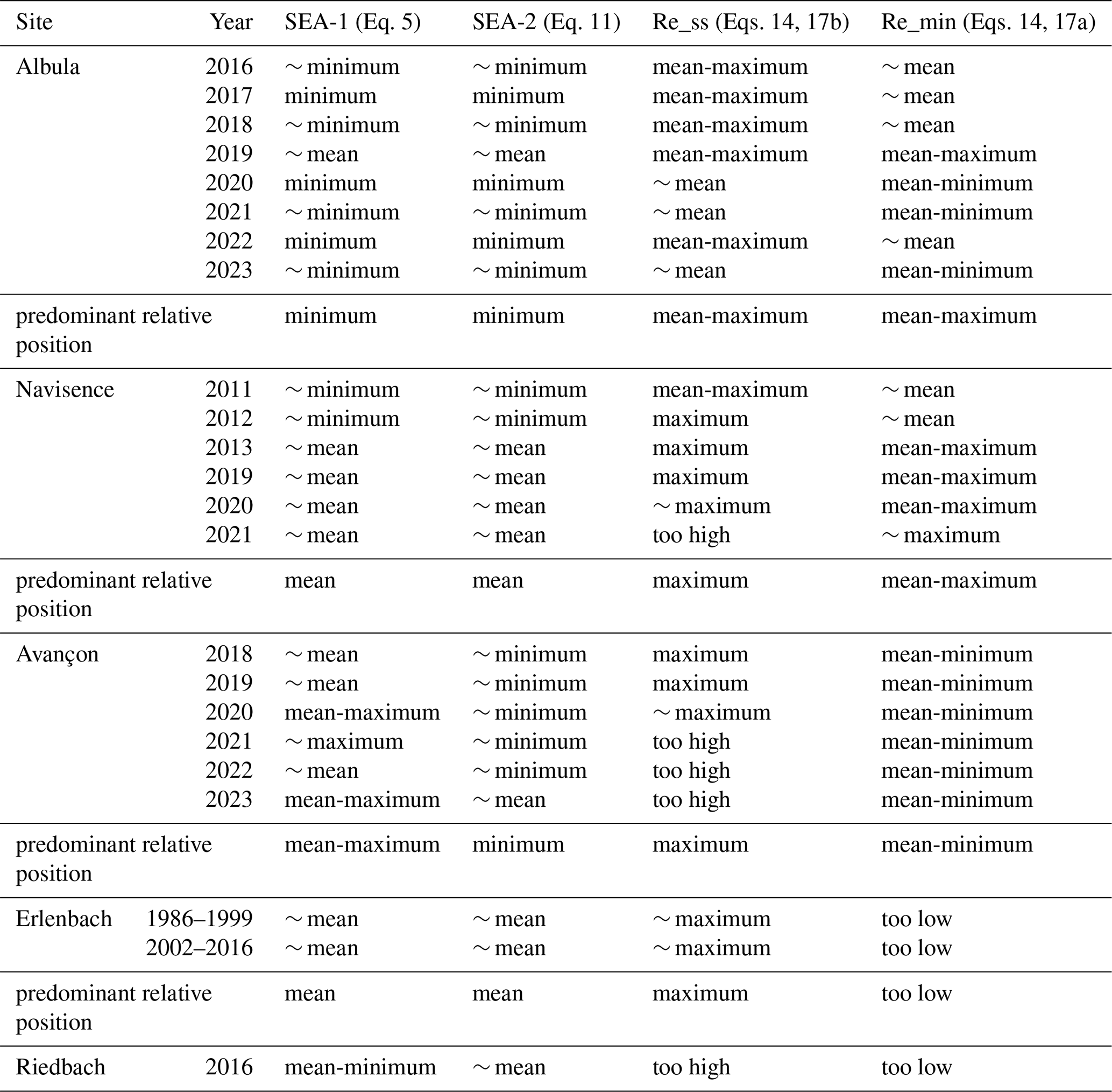
A qualitative comparison was made for the five streams of this study in Table D1 (Appendix D) where the approximate position of transport equations relative to measured data was assessed, including multiple year observations for four streams. This assessment shows that the predominant relative position of the SEA-1 and SEA-2 equations is in the “minimum – mean” range (except for the Avançon); on the contrary, the predominant relative position of the Re_ss and Re_min equations is in the “mean – maximum” range (except for the Riedbach). For this limited number of cases, this comparison would suggest that the Re_ss equation (Eqs. 14, 17b) tends to provide maximum bedload transport predictions in most steeper streams, and the SEA equations (Eqs. 5, 11) tend to provide medium to minimum or mean predictions in the steeper streams.

5 Conclusions

This study examined how bedload transport may vary in time and space. The analysis was based on continuous and long-term bedload transport surrogate measurements in several Swiss mountain streams using the Swiss Plate Geophone monitoring system. This indirect measuring system had been calibrated in previous studies to produce reliable estimates of bedload transport rates. The main findings and conclusions of the study are summarized as follows.

1. Bedload transport changes significantly during shorter time intervals such as a few weeks in larger streams or over a number of sediment-transporting flow events in a small mountain torrent. This variability was quantified in terms of the steepness and the reference shear stress of the two types of bedload transport equations proposed by Schneider et al. (2015a): one based on total bed shear stress and the other on a reduced bed shear stress formulation.

2. When bedload transport was aggregated yearly, i.e. over longer time scales, predictions from the above-mentioned equations agreed with measured values roughly within a factor of three, although some streams consistently showed over- or under-estimates. A potentially important finding for engineering applications is that yearly aggregated bedload masses depended approximately linearly on a simple measure of flow intensity, namely the integrated excess discharge multiplied with a normalized peak discharge.

3. The variability of the steepness and the reference shear stress is roughly in a similar range to that observed in a comprehensive study by Recking et al. (2016), which included direct bedload transport measurements from more than 100 streams; however, this only applies when channel slopes larger than about 2 % are considered. For the streams with channel slopes smaller than about 2 %, the Recking-study determined steepness values that are generally smaller than those found for the four Swiss streams and a data set in Schneider et al. (2015a), possibly due to a higher availability of fine particles in flatter streams.

4. The original form of the Meyer-Peter and Müller bedload transport equation is not suitable for bedload calculations over the entire discharge range and in particular for small and intermediate flow intensities in the vicinity of the critical dimensionless shear stress, because there is a step-like discontinuity in this range. An exponential form of the Meyer-Peter and Müller equation is more similar to the reference shear-stress based formulations (used in this study) and performs better in this range. However, a characteristic steepness of this equation is at the edge of the values resulting from the application of the bedload transport equation of Schneider et al. (2015a) based on total bed shear stress.

Appendix A: Flow resistance calculations

All flow resistance calculations are based on discharge-based equations using the following dimensionless variables for velocity $U^{\ast \ast }$ and for unit discharge $q^{\ast \ast }$ (Rickenmann and Recking, 2011):

$$\begin{array}{}\text{(A1)}& {\displaystyle }{U}^{\ast \ast }=U/\sqrt{gS{D}_{\mathrm{84}}}\text{(A2)}& {\displaystyle }{q}^{\ast \ast }=q/\sqrt{gS{D}_{\mathrm{84}}^{\mathrm{3}}},\end{array}$$

where U = mean flow velocity, S = channel slope D₈₄ = characteristic grain size of the bed surface for which 84 % of the particles are finer, q = unit discharge, and g gravitational acceleration.

For the Erlenbach, the hydraulic calculations were carried out with an equation given in Nitsche et al. (2012, Fig. 5d therein), based on dye tracer measurements made in the lowermost reach:

$$\begin{array}{}\text{(A3)}& U^{\ast \ast }=\mathrm{1.49}{q}^{\ast {\ast }^{\mathrm{0.6}}}\end{array}$$

For the Riedbach, the hydraulic calculations were carried out with an equation given in Schneider et al. (2016), also based on dye tracer measurements made in the lowermost reach:

$$\begin{array}{}\text{(A4)}& U^{\ast \ast }=\mathrm{1.74}{q}^{\ast {\ast }^{\mathrm{0.6}}}\end{array}$$

For the other three sites Albula, Navisence, and Avançon, the following equation of Rickenmann and Recking (2011) was used:

$$\begin{array}{}\text{(A5)}& U^{\ast \ast }=\mathrm{1.443}{q}^{\ast {\ast }^{\mathrm{0.6}}}{\left(\mathrm{1}+(q^{\ast \ast }/\mathrm{43.78}{)}^{\mathrm{0.8214}}\right)}^{-\mathrm{0.2435}}\end{array}$$

The unit discharge q was determined for a mean width for a given flow depth in the trapezoidal cross-section, and bank resistance was accounted for by reducing q with the ratio of the hydraulic radius r_h to the flow depth h.

Appendix B: Summary of bedload transport equations and interrelation of steepness exponents

Table B1 Summary of bedload transport equations and interrelation of steepness exponents. The expression f() denotes function of the variables in parenthesis. See Appendix E for a list of variables.

Appendix C: Variability of annual ratios of calculated to observed bedload masses: quantitative results

A graphical example for the determination of the ratios r_{t_incQ} and r_{r_incQ} with a linear model fitted to the function Cumsum (Q_bx) vs. Cumsum (Q_bM), x = tot or red, for the flow intensities ${\mathit{\tau }}_{D_{\mathrm{50}}}^{\ast }$ = > 1.1 ${\mathit{\tau }}_{\mathrm{r}{D}_{\mathrm{50}}}^{\ast }$, is given for the Albula in 2019 in Fig. C1a. The values of r_{t_incQ} and r_{r_incQ} were then compared with the chronologically determined ratios Cumsum (Q_bx) to Cumsum (Q_bM), i.e. the r_{t_chron} and r_{r_chron} values, for each year. Figure C1b illustrates this for the Albula in 2019. This allowed to derive the approximate duration from the beginning of the transport season to the time point after which the r_{x_chron} values were within about a factor of 3 above or below the r_{x_incQ} values, x = t or r. These limiting deviations are illustrated by dashed and dotted lines in Fig. 7b, indicating that the relative agreement of calculated to observed bedload masses only varied in a limited range after this time point. In the Supplement similar diagrams are given for all years of the Albula (Figs. S4 to S11), the Navisence (Figs. S14 to S19), the Avançon (Figs. S22 to S27), and the Erlenbach (Figs. S29 to S30).

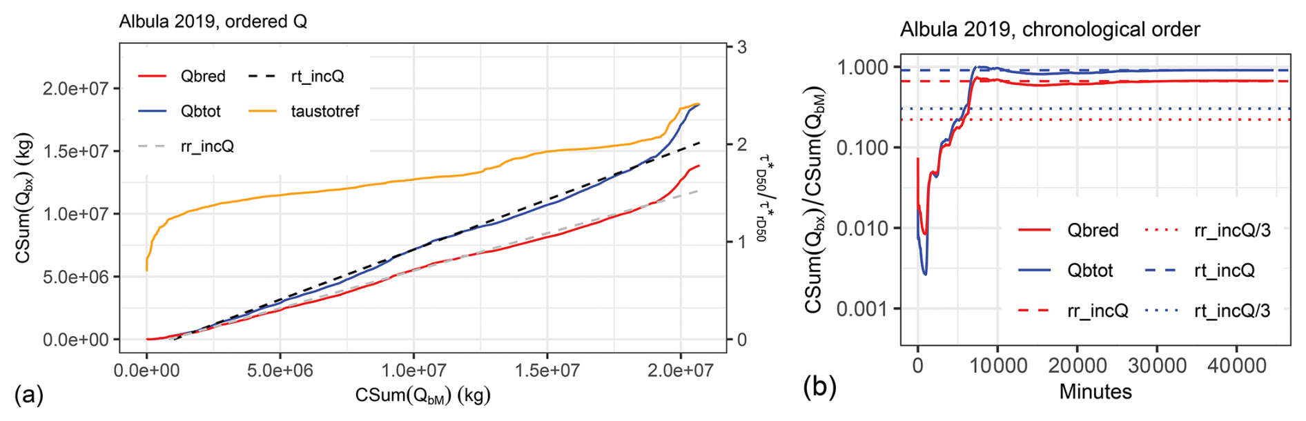
Figure C1 Albula, summer 2019. Example of a good agreement of a linear model (dashed black and gray lines) for the cumulative sum of calculated (CSum(Q_bx)) vs. measured (CSum(Q_bM)) bedload masses. In panel (a) the values were ordered according to increasing discharge Q, and the increase in relative flow intensity is shown with the ratio ${\mathit{\tau }}_{D_{\mathrm{50}}}^{\ast }/{\mathit{\tau }}_{\mathrm{r}{D}_{\mathrm{50}}}^{\ast }$ (taustotref). In panel (b) the values are summed up in chronological order.

Table C1 Annual mean ratios of calculated to observed bedload masses, and results of cumulative sum analysis. See text and list of symbols for meaning of variables. A full list with all the individual values for each stream is given in the Supplement (Tables S2, S3, S4, S5).

Appendix D: Position of transport equations relative to measured data

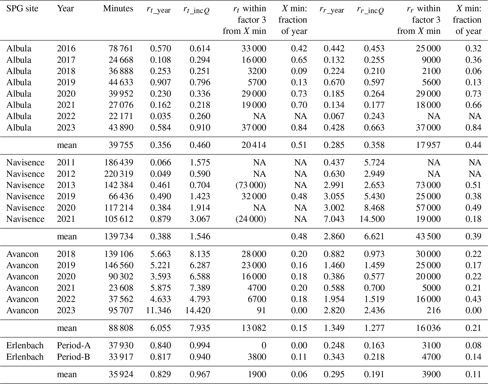
Table D1 Multiple year observations: approximate position of transport equations relative to measured data. The assessment of the relative position is based on the graphs in the Supplement, i.e. for the Albula (Figs. S1, S2, S3), for the Navisence (Figs. S12, S13), for the Avançon (Figs. S20, S21), and for the Erlenbach (Fig. S28). For the Riedbach see Fig. 3 in the main text.

Appendix E: List of variables and abbreviations for data sets

Ac	size of catchment area (km2) at the location of the SPG measuring site
Dxx	grain size of the bed surface for which xx % of the particles are finer
IMP	impulse counts per minute (using the SPG system)
kisp	calibration coefficients determined for each survey interval at the Erlenbach
ksite	calibration coefficients determined for the Albula, Navisence, and Avançon
m	Exponent in Eq. (2), general term including mtot from $W_{\mathrm{tot}}^{\ast }$ analysis and mred from $W_{\mathrm{red}}^{\ast }$ analysis
MQbM	sum of QbM per year, multiplied with 60 s, to give the yearly transported bedload mass
MQbred	sum of Qbred per year, multiplied with 60 s, to give the yearly calculated bedload mass
MQbtot	sum of Qbtot per year, multiplied with 60 s, to give the yearly calculated bedload mass
Q	water discharge (m3 s−1)
Qmax	maximum water discharge (m3 s−1) in a given year
Q1.1	water discharge (m3 s−1) corresponding to a dimensionless shear stress ${\mathit{\tau }}_{D_{\mathrm{50}}}^{\ast }$ = 1.1 ${\mathit{\tau }}_{\mathrm{r}{D}_{\mathrm{50}}}^{\ast }$ (Table 3)
qb	volumetric bedload transport rate per unit width (m2 s−1)
Qbm	measured bedload transport rate (Eq. 1) (kg s−1)
QbM	measured bedload transport rate, zero values replaced by mean with neighboring non-zero values (kg s−1)
Qbred	calculated bedload transport rate, based on the reduced (effective) shear stress (Eq. 9)
Qbtot	calculated bedload transport rate, based on the total shear stress (Eq. 2)
Qbz	measured bedload transport rate, including zero values
Qc	critical discharge for begin of substantial bedload transport (Sect. 4.4)
Qc2a, Qc2b	begin of phase-2 transport according to Bathurst (2007) (Table 3)
Qmax	annual peak discharge
rt_chron	ratio of Cumsum (Qbtot) $/$ Cumsum (Qbm) [Eq. 30a]
rr_chron	ratio of Cumsum (Qbred) $/$ Cumsum (Qbm) [Eq. 30b]
rt_incQ	slope of linear model between Cumsum (Qbtot) and Cumsum (Qbm) [Eq. 29b]
rr_incQ	slope of linear model between Cumsum (Qbred) and Cumsum (Qbm) [Eq. 29b]
rt_year	ratio of $M{Q}_{\mathrm{btot}}/M{Q}_{\mathrm{bM}}$ [Eq. 28a]
rr_year	ratio of $M{Q}_{\mathrm{bred}}/M{Q}_{\mathrm{bM}}$ [Eq. 28b]
R2	squared Pearson correlation coefficient
$s={\mathit{\rho }}_{\mathrm{s}}/\mathit{\rho }$	relative sediment density, with ρs = sediment density and ρ = water density
S	channel slope of natural channel-reach upstream of SPG site
S′	reduced energy slope (associated with a reduced or effective shear stress)
u∗	the shear velocity (m s−1)
U	mean flow velocity (Appendix A)
w	channel width
W∗	dimensionless bedload transport rate, $W^{\ast }=(s-\mathrm{1})g{q}_{\mathrm{b}}/u^{\ast \mathrm{3}}$ [Eq. 13]
Φb	dimensionless bedload transport rate, ${\mathrm{\Phi }}_{\mathrm{b}}=q_{\mathrm{b}}/\sqrt{(s-\mathrm{1})g{D}_{\mathrm{50}}^{\mathrm{3}}}$ [Eq. 21]
Φb84	dimensionless bedload transport rate, ${\mathrm{\Phi }}_{\mathrm{b}}=q_{\mathrm{b}}/\sqrt{(s-\mathrm{1})g{D}_{\mathrm{84}}^{\mathrm{3}}}$ [Eq. 15]
τ∗	dimensionless total bed shear stress, τ∗ = ($g\mathit{\rho }{r}_{\mathrm{h}}S)/(g\mathit{\rho }(s-\mathrm{1})D_{xx})$
τ′	dimensionless reduced or effective bed shear stress, τ′ = $\left(g\mathit{\rho }{r}_{\mathrm{h}}{S}^{\prime }\right)/\left(g\mathit{\rho }\right(s-\mathrm{1}\left)D_{xx}\right)$
${\mathit{\tau }}_{\mathrm{c}}^{\ast }$	dimensionless critical shear stress (at beginning of motion)
${\mathit{\tau }}_{D_{\mathrm{50}}}^{\ast }$	dimensionless total bed shear stress (for $W_{\mathrm{tot}}^{\ast }$, Eq. 2), with reference to D50
${\mathit{\tau }}_{D_{\mathrm{50}}}^{\ast \prime }$	dimensionless reduced bed shear stress (for $W_{\mathrm{red}}^{\ast }$, Eq. 9), with reference to D50
${\mathit{\tau }}_{\mathrm{Re}\mathrm{84}}^{\ast }$	dimensionless total bed shear stress (for Φb84, Eqs. 14, 19), with reference to D84
${\mathit{\tau }}_{\mathrm{ref}}^{\ast }$	dimensionless reference shear stress, general term including ${\mathit{\tau }}_{\mathrm{r}{D}_{\mathrm{50}}}^{\ast }$ from $W_{\mathrm{tot}}^{\ast }$ analysis, ${\mathit{\tau }}_{\mathrm{r}{D}_{\mathrm{50}}}^{\ast \prime }$ from $W_{\mathrm{red}}^{\ast }$ analysis, and ${\mathit{\tau }}_{\mathrm{rRe}}^{\ast }$ in Eq. (14, 19)
${\mathit{\tau }}_{\mathrm{rRe}\mathit{\_}min}^{\ast }$	dimensionless reference shear stress of Recking (2013), Eq. (17a), for streams with limited sediment availability, resulting in a “minimum” bedload transport level
${\mathit{\tau }}_{\mathrm{rRe}\mathit{\_}\mathrm{ss}}^{\ast }$	dimensionless reference shear stress of Recking (2012), Eq. (17b), for streams with a high sediment supply, resulting in a “high” bedload transport level
CH_TV	data set of CH-streams (this study) with analysis temporal variation (TV) of bedload transport
REA_BT	data set of Recking et al. (2016), for which β and ${\mathit{\tau }}_{\mathrm{ref}}^{\ast }$ (BT) were optimized for Eq. (14)
SEA_HS	data set of Schneider et al. (2015), “main data set” of 14 steep streams (SS)
SEA_SS	data set of Schneider et al. (2015), “HS (Helley-Smith) data set” of 21 streams