Coastal process understanding through automated identification of recurring surface dynamics in permanent laser scanning data of a sandy beach

Four-dimensional (4D) topographic datasets are increasingly available at high spatial and temporal resolution, particularly from permanent terrestrial laser scanning (PLS) time series. These data offer unprecedented opportunities to analyse rapid and complex morphological processes occurring in sandy coastal environments, such as sandbar welding or bulldozer activity, as well as their longer-term impacts on sandy beaches. However, studying these processes requires the extraction and recognition of recurrent topographical surface dynamics across time, which in turn demands novel, automated methods. This study presents a novel workflow that combines 4D objects-by-change (4D-OBCs) with unsupervised classification using Self-Organizing Maps (SOMs) and hierarchical clustering. Applied to a three-year PLS time series comprising 21 194 hourly point clouds, the method identifies 4412 instances of short-term surface dynamics. These are organized into two SOMs (64 nodes each) and further grouped into 31 clusters representing distinct dynamic types, such as berm deposition, large-scale backshore erosion, and human interventions (e.g., bulldozer activity). The classification results enable detailed spatiotemporal analyses of coastal morphodynamics. The SOM topology reveals seasonal patterns in surface activity, where, for example, winter is dominated by erosional activity over the whole beach but depositional activity mainly occurs in the intertidal area. The broader clusters facilitate interpretation of environmental responses and identification of changes in cross-shore zonation of types of dynamics, like berm formation. This approach demonstrates the potential of integrating PLS and unsupervised learning to characterize complex surface dynamics, through a fully automated extraction and classification workflow. While the interpretation of clusters and their relation to environmental variables in this study is performed through expert-based analysis, the methods provide a framework for targeted, data-driven investigation and prediction of morphodynamic processes in high-resolution 4D remote sensing datasets.

1 Introduction

Coastal zones are among the most densely populated regions worldwide, with large socioeconomic and ecological value (Small and Nicholls, 2003; Lansu et al., 2024). Approximately one third of these coastlines are sandy ecosystems, consisting of beaches and dunes (Luijendijk et al., 2018). These buffers play a critical role in mitigating coastal hazards such as storm surges and erosion, in order to protect inland regions and important ecological habitats (Christiaanse et al., 2024). However, the resilience of sandy coastal systems is increasingly under pressure due to climate change and human interventions (Vousdoukas et al., 2018; Lansu et al., 2024). Rising sea levels, changing storm patterns, and human-driven coastal development alter sediment budgets and feedback dynamics (Mentaschi et al., 2018), leading to the degradation or loss of natural buffers. This phenomenon, known as coastal squeeze, threatens the long-term habitability of low-lying coastal areas (Vousdoukas et al., 2020).

To manage and anticipate the future of beach ecosystems, it is essential to monitor and understand the morphodynamic behaviour of sandy coastlines (Woodroffe et al., 2025; Christiaanse et al., 2025). This behaviour is a function of sand transport, which governs both short-term surface dynamics and consequently longer-term morphological evolution. These sand transport processes, however, are driven by complex interactions between hydrodynamic, aeolian, bio-geophysical, and anthropogenic forcing (i.e. water, wind, vegetation, and human activity), with periodic feedbacks across a range of spatiotemporal scales (Splinter and Coco, 2021; Chowdhury et al., 2023; Tereszkiewicz and Ellis, 2025). The latter makes observing the processes particularly complex .

For example, seasonal cycles exist of the build-up, transport and ablation of sandbars, driven by daily variations in wave height, wave direction and water level (Dubarbier et al., 2015; Vos et al., 2020). Depending on the strength of these cycles, this may lead to annual net accretion or erosion on the beach (Cohn et al., 2017). In the longer term (decades), the inland dunes may appear to grow as a function of a cycle of aeolian transport and incidental storm erosion (Cohn et al., 2019). However, as identified by De Vries et al. (2014), aeolian sediment transport toward the dune is often limited by supply or, in other words, limited by the availability of sediment in the fetch region on the beach (Delgado-Fernandez, 2010). Consequently, short-term changes in the cycle of sandbar transport and beach berm welding, and resulting shoreline position might have great impact on the longer-term development of the beach-dune system (Cohn and Anderson, 2025). This shoreline positioning can be further impacted by longshore sediment transport in the surf zone, which also show strong seasonal and decadal variability (Silva et al., 2012; Anderson et al., 2018), and alter availability of sand for cross-shore transport through redistribution (Palalane and Larson, 2019). On top of this, the beaches are increasingly adapted by humans through nourishments (De Schipper et al., 2020), and incident-driven bulldozing that flattens the beach for accessibility and infrastructure protection (Lazarus and Goldstein, 2019). The presence or absence of vegetation (Moore et al., 2025) and buildings (Vos et al., 2024) also further influences the complexity of these beach-dune sand transport and deposition processes. Understanding interactions across temporal scales is therefore essential for anticipating the effects of climate change and human impact on long-term development of sandy coast environments.

Capturing and interpreting all these interactions requires frequent, and prolonged monitoring of topographic changes with high spatial resolution. In the past, monitoring has mainly been done through profiling of the coast at alongshore intervals of several hundreds of meters. Decades of labour-intensive fieldwork created extensive datasets of topographic dynamics (Turner et al., 2016), to some extent offering the basis to understand multi-scale interactions of coastal dynamics. However, the time- and labour-intensive nature of this manual monitoring puts limits on its spatial data density and temporal frequency. Consequently, the data cannot fully describe detailed 3D interactions of short-term processes.

Recent advances in remote sensing technologies opened the potential to acquire spatiotemporally dense data across large coastal domains. In particular, satellite imagery is now widely used to extract morphodynamic indicators such as shorelines and dune toes, which provide valuable insights into large-scale and long-term coastal landscape evolution (Vos et al., 2023a; Castelle et al., 2024). These indicators are effective for tracking erosional trends and regional coastal behaviour, but they remain proxies of the total morphodynamic response and provide little information on the underlying processes that govern landscape change. More detailed datasets of morphodynamics, derived from UAV surveys, aerial LiDAR scans, GNSS surveys, or terrestrial laser scanning (TLS), are still limited in either their spatial resolution and detail (Abdulsalam et al., 2025), temporal frequency (De Almeida et al., 2019), or temporal coverage (Lindenbergh et al., 2011). These factors lower their efficacy in understanding small-scale, short-term dynamics (hours to months) and their effect on longer-term (years to decades) morphological trends. As a result, scale-dependent feedbacks between noise-level dynamics and cumulative change remain underrepresented in studies and their derived coastal models (Walker et al., 2017; Ranasinghe, 2020).

Advances in permanent terrestrial laser scanning (PLS) offer more promising opportunities for capturing high-resolution topography across multiple spatiotemporal scales (Eitel et al., 2016; Lindenbergh et al., 2025). PLS systems continuously capture high-resolution (cm-level), high-frequency (hours to days) 3D point clouds over extended periods (> years). They are consequently generating dense 3D time series datasets allowing to identify both rapid elevation changes and their cumulative effects over time (Lindenbergh et al., 2025). This temporal coverage positions PLS as a unique tool for monitoring and understanding the evolution of dynamic coastal landscapes comprehensively.

Yet, using PLS data integrally without extensive manual interpretation remains challenging. Datasets contain up to tens of thousands of scans (O'Dea et al., 2019; Vos et al., 2023c), each comprising millions of 3D points. Traditional bitemporal change detection methods, such as DEM differencing or M3C2 (Lague et al., 2013), can be used to analyse the long-term signal of dynamics in selected epochs of the dataset, but for hour-to-hour analysis such bitemporal methods become impractical and are limited in their performance with respect to signal-to-noise ratio and detectability of different process scales (Anders et al., 2020). Several methods have been proposed to leverage dense temporal sampling of PLS for change detection in various environmental settings (Anders et al., 2021; Kuschnerus et al., 2021; Winiwarter et al., 2023; Kuschnerus et al., 2024a; Tabernig et al., 2025a, b). For the identification of coastal surface dynamics specifically, Kuschnerus et al. (2021) applied unsupervised classification to full elevation time series, enabling the identification of areas with similar overall dynamics. While valuable for identifying widespread coastal patterns, this approach cannot easily group similar short-term events that occur at different times, does not include spatial segmentation, and requires an a priori choice of cluster numbers. A follow-up study by Kuschnerus et al. (2024a) introduced temporal segmentation of elevation trends, which better identifies short-term dynamics, but still lacks spatial grouping of similar behaving areas.

The 4D objects-by-change (4D-OBC) method (Anders et al., 2021) addresses the main limitations by extracting spatiotemporal extents of homogeneous elevation change, such as the build-up and transport of an intertidal bar. However, for an hourly PLS dataset of 6 months, the resulting set of 4D-OBCs still contains over 2000 individual dynamics. These 4D-OBCs are a full, unorganized set of surface dynamics objects with a specific start and end time, and a certain spatial extent, but without semantic meaning, i.e., similar dynamics and different moments in time are not identified together. The task of identifying similar types of relevant dynamics in the full dataset as objects of interest is still needed before one can analyse the characteristics, conditions, and impacts of specific short-term dynamics at different moments in time. With PLS datasets growing to several years of data, manual analysis is in general too time- and labour-intensive. This highlights the need for automated and unsupervised approaches that group similar dynamics, such as bar migration, berm formation, or bulldozer deposits, across time and space (Hulskemper et al., 2022; Wang and Anders, 2025).

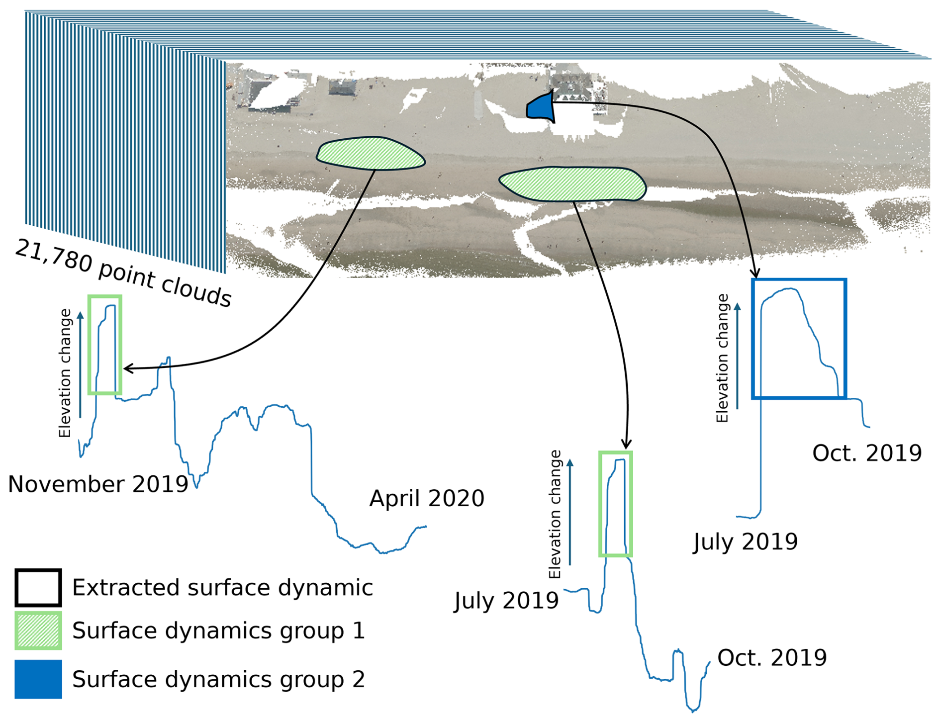
Figure 1 Schematic demonstrating the goal of this research in grouping similar short-term surface dynamics occurring at different moments in time, to study their characteristics. Visualisation is based on a point cloud from the permanent laser scanning dataset, colourised using aerial photographs provided by the Dutch government (https://www.beeldmateriaal.nl/dataroom, last access: 5 May 2026).

To leverage the full potential of PLS data for analysis of scale-dependent interactions, we require methods that can: (1) reduce data complexity without discarding information on important spatiotemporal processes, (2) extract temporal and spatial extents of surface dynamics of short temporal scales (hours to months, black boxes in Fig. 1), and (3) identify similar types of surface dynamics at different moments in time based on their spatiotemporal characteristics (green boxes in Fig. 1). Methods that fulfil these requirements are necessary to link appearance of types of surface dynamics to environmental drivers, to support comparative analyses, and to ultimately understand how short-term processes contribute to long-term morphological change.

In this study we address these challenges to answer the question: how can short-term surface dynamics in sandy coastal systems be extracted, grouped and linked to environmental variables? To this end we develop a workflow that combines spatiotemporal segmentation using 4D-OBCs (Anders et al., 2021) with unsupervised classification techniques, and environmental variables. This workflow is applied to a long-term PLS dataset of 21 194 hourly point clouds collected over 3 years at a high-energy urbanized sandy beach (Vos et al., 2023c). Short-term surface dynamics are here regarded as changes in the topography that have a time-span of up to several months. Environmental variables are defined as any potential forces for change on the beach, be it natural or anthropogenic, such as wind or bulldozer works.

The main contributions are as follows. We provide a method that allows for identification and grouping of similarly behaving short-term surface dynamics even when they occur at different moments in time. This enables systematic study of the environmental, sequential, and periodic characteristics of different surface dynamics, allowing researchers to connect observed morphological changes with the processes and conditions that drive them. We demonstrate the effectiveness of the method in classifying and organizing the PLS dataset into known and previously unidentified types of short-term surface dynamics, but also artefacts. Additionally, we show different ways in which this structured dataset enables the exploration of individual types of surface dynamics and their temporal variations in relation to environmental and seasonal changes. This approach provides a new means to leverage high-frequency topographical datasets for coastal research. In future work, the structured dataset of grouped surface dynamics can be linked to environmental drivers through automated data-driven methods, such as threshold analysis, time series correlation, or physics-informed machine learning, enabling systematic and scalable investigation of causal relationships of surface dynamics. The dataset used in this study is acquired in a PLS setup, but the method is generalizable to any time series of topographic point clouds, regardless of acquisition platform, such as multitemporal UAV, airborne or satellite topographic measurements, as long as sufficient temporal frequency and spatial resolution are available to detect the target surface dynamics.

2 Materials

2.1 Permanent laser scanning dataset

In a PLS setup, a TLS is permanently mounted and acquires elevation data as point clouds over regular intervals for an extended period of time. For this study, a dataset of 21 780 hourly point clouds is used, acquired with a Riegl VZ2000 at Noordwijk, the Netherlands (Fig. 2) between 11 July 2019 and 21 July 2022 (Vos et al., 2023c). The scanner was positioned on a hotel at 55.575 m above Normaal Amsterdams Peil (approximate Mean Sea Level in the Netherlands, MSL). Figure 3 shows a coloured version of one point cloud in the time series. Elevation measurements of the dune area, backshore, and part of the intertidal area are obtained. Spatial gaps in the data exist because of occlusion from the single viewpoint of the permanent TLS position. Consequently, the dune foot cannot be observed in the data. Details on the data characteristics (e.g., point density and accuracy) and setup can be found in Vos et al. (2022).

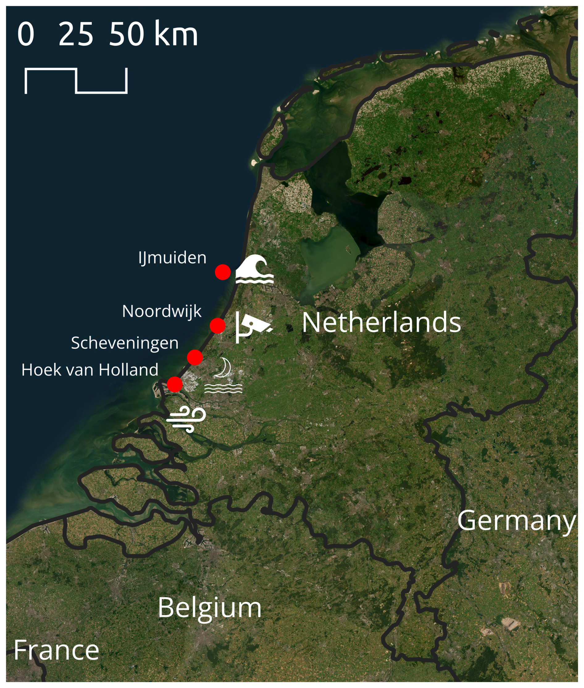
Figure 2 Measurement locations in the Netherlands for permanent laser scanning data (Noordwijk), wave data (IJmuiden), water level (Scheveningen) and meteorological data (Hoek van Holland). The background map uses ESRI World Imagery (Powered by Esri, © ESRI, Maxar, Earthstar Geographics, and the GIS User Community).

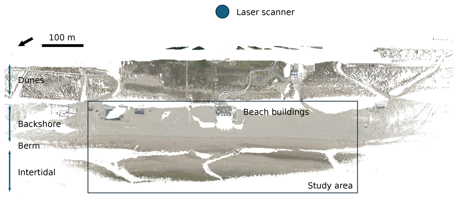
Figure 3 Permanent laser scanning point cloud of the study area indicating the main morphological beach units and cross-shore area featuring buildings. The scan is coloured using Dutch national aerial photos (https://www.beeldmateriaal.nl/dataroom).

Several pre-processing steps are undertaken before surface dynamics are extracted from the point cloud time series. First, the XYZ values of each point cloud are corrected for scanner tilt using transformation matrices as provided with the dataset at 4TU.research data (Vos et al., 2023c). This reduces the systematic error between consecutive point clouds due to, for example, heat effects and storm conditions (Voordendag et al., 2023; Kuschnerus, 2024). There are some temporal gaps in the dataset of which the longest is 1.5 months. These occur due to system failure, periods of bad weather, or maintenance. Some point clouds in the dataset were found to be noisy, containing points over the whole field of view, mostly below the actual topography. These point clouds are removed by filtering based on thresholding of the lowest 10th percentile of the z-value of the point clouds. If this is lower than −60 m in the local coordinate system established by the scanner position, thus corresponding to −4.425 m a.m.s.l., the point cloud is not used. Finally, the remaining 21 194 point clouds are cropped to contain only the area indicated in Fig. 3. The dune area is cropped out, as the vegetation obscures most of the sand transport. The far intertidal area is not used as only little data is available from this area, because the near-infrared LiDAR does not penetrate water (Höfle et al., 2009).

2.2 Environmental dynamics

The environmental dynamics considered in this study are obtained from hydrodynamic and meteorological measurements. Their relation to surface dynamics is assessed through several parameters representative of wave, water level and wind dynamics, namely, the significant wave height (H_s), period of significant waves (T_p), the water level (W_h), mean wind speed (u), and the wind direction (θ). These dynamics are chosen as they are input variables in most hydro- and morpho- dynamic models (Lesser and Roelvink, 2004; Roelvink and Costas, 2019; Van Westen et al., 2024). Other possibly important variables like wave direction, precipitation or socioeconomic factors like the crowdedness are not considered in this study, but could be added in future work.

For the analysis the wind direction is converted to the direction in degrees with 0° in along shore direction (θ_coast). The sine of the angle then gives a continuous variable with 1 being seaward wind direction, 0 for wind parallel to the coast (in both directions), and −1 for landward wind.

The meteorological dynamics are obtained at an hourly interval at Hoek van Holland by the Dutch Meteorological Institute (KNMI, 2024). The hydrodynamics are also provided hourly. The parameters related to wave dynamics are measured at IJmuiden and the water level at Scheveningen. Both by the Public Works and Water Management Department of the Netherlands (Rijkswaterstaat, 2024). They match the acquisition time of each point cloud. Locations of the different measurements stations are visualised in Fig. 2. The monitoring stations are located at distances up to ∼ 35 km from the PLS site. Meteorological and hydrodynamic conditions along this stretch of the Dutch North Sea coast are, however, highly spatially coherent at the timescales considered in this study. Wind speed over the southern North Sea has a decorrelation length on the order of hundreds of kilometres for daily variability (Sušelj et al., 2010), with Hoek van Holland and IJmuiden showing similar wind statistics (Coelingh et al., 1998). Wave conditions along the Dutch coast are also spatially homogeneous, with observed deviations in mean significant wave height on the order of only 0.2 m (Wijnberg, 2002).

3 Methods

The methods presented in this research are developed to identify and group similar types of short-term surface dynamics (e.g., intertidal bar build-up + erosion/migration, berm depositions + consecutive erosion) present in long point cloud time series of a sandy beach, and enable systematic investigation of their characteristics, conditions, temporal sequences, and periodicity. The method consists of four main steps (Fig. 4).

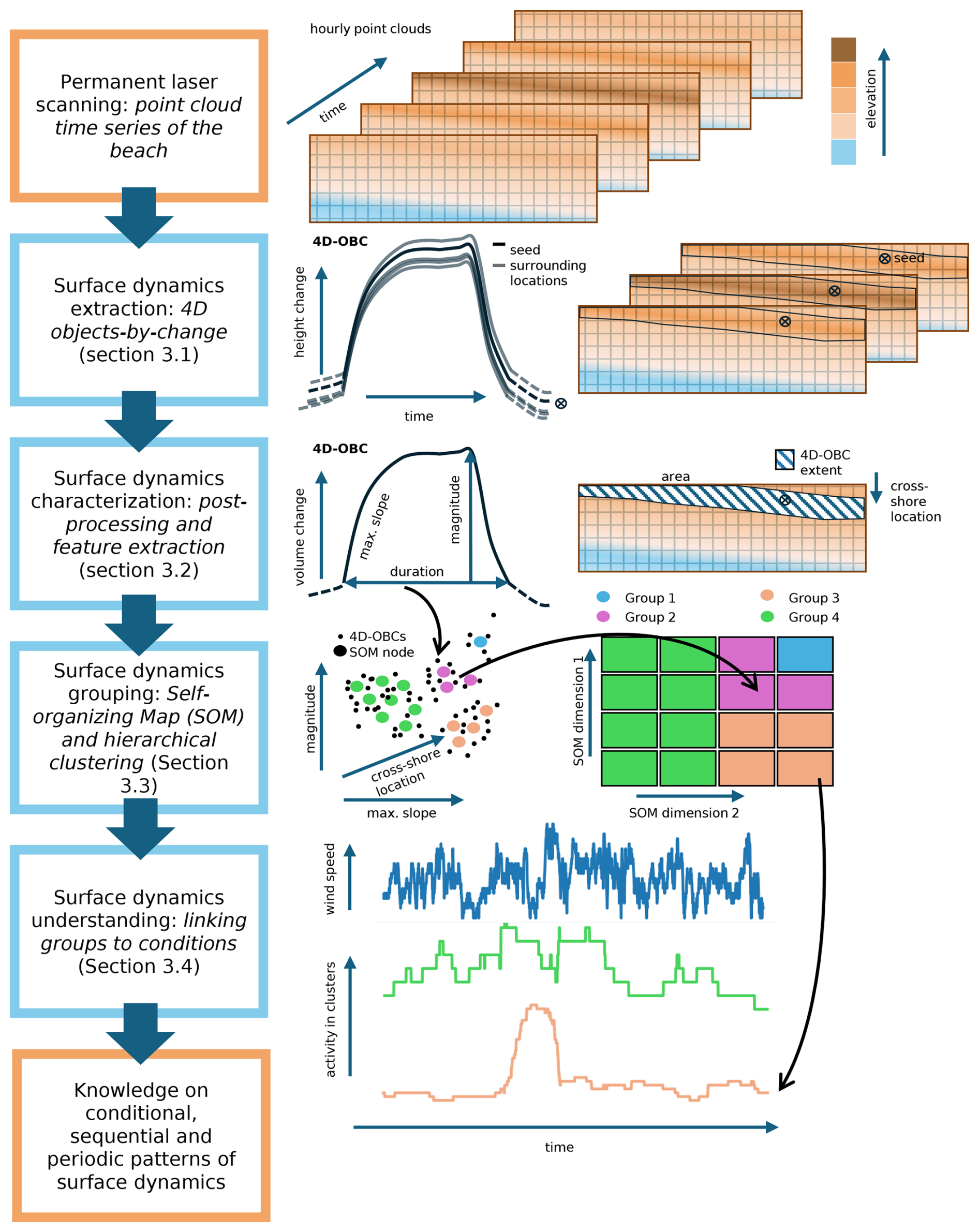
Figure 4 Overview of full workflow for surface dynamics grouping and understanding from dense permanent laser scanning point cloud time series.

First we automatically extract the surface dynamics from the point cloud time series as 4D objects-by-change (4D-OBCs). Second, features are derived from the extracted 4D-OBCs. Third, these features are used in an automated and unsupervised clustering workflow to obtain groups of 4D-OBCs at two levels of detail, based on a Self-organizing Map (SOM) and subsequent hierarchical clustering. Fourth, representative time series are obtained for each of the clusters. These are then further analysed to identify dominant environmental conditions under which certain types of dynamics are present. Finally, we present our strategy to evaluate the found groups of surface dynamics, and their relations to environmental conditions.

3.1 Step 1: extraction of surface dynamics as 4D objects-by-change

From the point cloud time series of a permanent laser scanner, surface dynamics as 4D-OBCs are extracted. A 4D-OBC represents a spatiotemporally confined surface dynamic event like the deposition and consecutive erosion or transport of an intertidal bar. In other words, it is an elevation change defined through a fixed timespan and with a fixed planimetric extent. These temporary surface dynamics are extracted through the 4D-OBCs algorithm, as available in the py4dgeo Python software (Anders et al., 2026). This algorithm consists of several steps, to extract a set of spatiotemporal segments (4D-OBCs) from a point cloud time series, which we explain in the context of the analysis of the work in Anders et al. (2021).

3.1.1 4D objects-by-change algorithm

Initially, the full point cloud time series is reduced to a time series of elevation changes on a set of corepoints. This is done through computation of the multiscale model-to-model cloud comparison distance (M3C2; Lague et al., 2013) of every cloud to a single reference scan. When this is done for every point cloud we obtain a 4D space-time array of elevation changes at the selected corepoints (e.g., Fig. 5a and b). We choose the corepoints as a regular grid with a 2D (planimetric) sampling distance of 1 m covering the beach and intertidal area. This spatial resolution is considered appropriate for the surface dynamics we aim to capture (> 10 m²). Morphological changes below this resolution fall within the positional uncertainty of the PLS and cannot be reliably distinguished from sensor noise (Kuschnerus et al., 2024b). We therefore do not consider them in the present analysis.

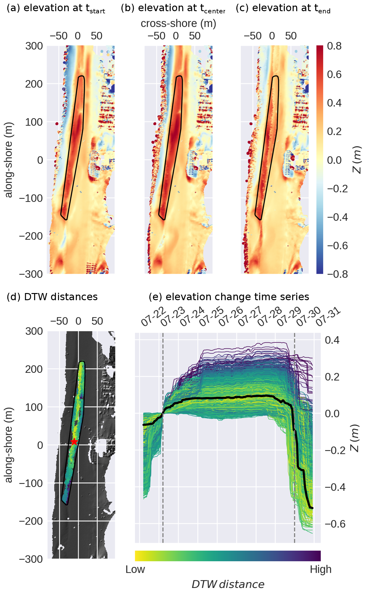
Figure 5 Spatial (a–d) and temporal (e) representation of a 4D object-by-change (4D-OBC). (a) Elevation change in corepoints with respect to the first epoch of the dataset at the start of the 4D-OBC. The convex hull around the 4D-OBC is coloured in black. (b) Elevation change at the central epoch of the 4D-OBC. (c) Elevation change at the last epoch of the 4D-OBC. (d) All points captured in the 4D-OBC (coloured area). The colours indicate the Dynamic Time Warping distance (DTW) to the seed time series (red star). (e) Time series of elevation change with respect to the start of the 4D-OBC, of the seed (in black), and other points incorporated in the 4D-OBC (coloured by DTW distance, corresponding to panel d). The temporal extent of the 4D-OBC lies between the two dashed lines.

The obtained time series are smoothed to further ensure outliers like objects and humans on the beach, and measurement errors are not affecting the 4D-OBC extraction. This smoothing is done using a temporal median averaging window of 168 h (1 week), following Anders et al. (2020, 2021), where it was found to effectively suppress sub-daily noise while preserving multi-day surface dynamics of geomorphological relevance. By design, changes occurring on timescales shorter than the window are not captured in the smoothed time series, this is a consequence of the chosen observation scale, consistent with the minimum detectable event duration of 24 h. In studies where higher-frequency reliable data is available, a shorter filtering window could be used. This filtering also interpolates temporal gaps in the data, e.g., when data is missing due to rainfall, tidal water level, or technical problems.

In the smoothed time series of the space-time array, breakpoints are detected to determine moments in time when change occurs. Each of these breakpoints can represent the onset of a temporary surface dynamic. The detection is done using a sliding temporal window with a width of 24 h. If the discrepancy between the median of the first and second half of the window exceeds a penalty-driven discrepancy, a breakpoint is detected (Truong et al., 2020). The 24 h window width ensures that breakpoints are detected at high sensitivity, however detecting changes at shorter windows is not deemed useful, because the subdaily scale is already mostly averaged through temporal smoothing.

Starting from each breakpoint, a temporal region is extended until the elevation of the point is back at the breakpoint elevation again. This extent is used as a seed candidate, which represents the temporal extent of a potential surface dynamic (Fig. 5d). The derivation of the extent is governed by two parameters: the minimum duration, and minimum absolute elevation change (i.e., magnitude). These parameters thus define partially the minimal spatiotemporal scale that a 4D-OBC can describe. In this study we only consider seeds with a duration of 12 h or more and a magnitude of 5 cm or more. Lower magnitudes are close to the standard error of the LiDAR data, and might thus be the result of measurement errors. Note that processes resulting in net elevation change such as dune growth or longer-term beach erosion trends are thus by design not captured in these seeds. The algorithm detects temporary deviations that return to a baseline elevation. The study of such longer-term or permanent geomorphic trends requires complementary analysis methods, such as bitemporal DEM differencing or elevation time series trend assessment (Kuschnerus, 2024).

From the temporal seeds, spatial regions are grown to complete the spatiotemporal extent of a surface dynamic (Fig. 5c). This is done by first sorting all the seeds based on their neighbourhood homogeneity, i.e., the coefficient of variation determined by the seed and its eight neighbouring locations based on the Dynamic Time Warping distance (DTW; Berndt and Clifford, 1994; Anders et al., 2021). Then, from the first seed, a region is grown by considering the DTW distance between the seed time series and its neighbours. If this distance is within an adaptive threshold (Anders et al., 2021), the time series is considered similar and the core point is added to the segment. The algorithm halts once no new point within the threshold distance is found; the spatiotemporal segment, or 4D-OBC is then completed. Thereafter the next seed in line is considered. If the region is smaller than a threshold t_area of 10 m² it is not used, which is a practical choice in terms of the spatial data resolution at hand and the size of target change processes. Reducing this threshold leads to a strong increase in the detected number of 4D-OBCs, most of which represent small-scale fluctuations at the margin of sensor precision (Vos et al., 2023b). A lower ranked seed is not considered if it is already within a previous spatiotemporal segment, to ensure no 4D-OBCs describe the same surface dynamic.

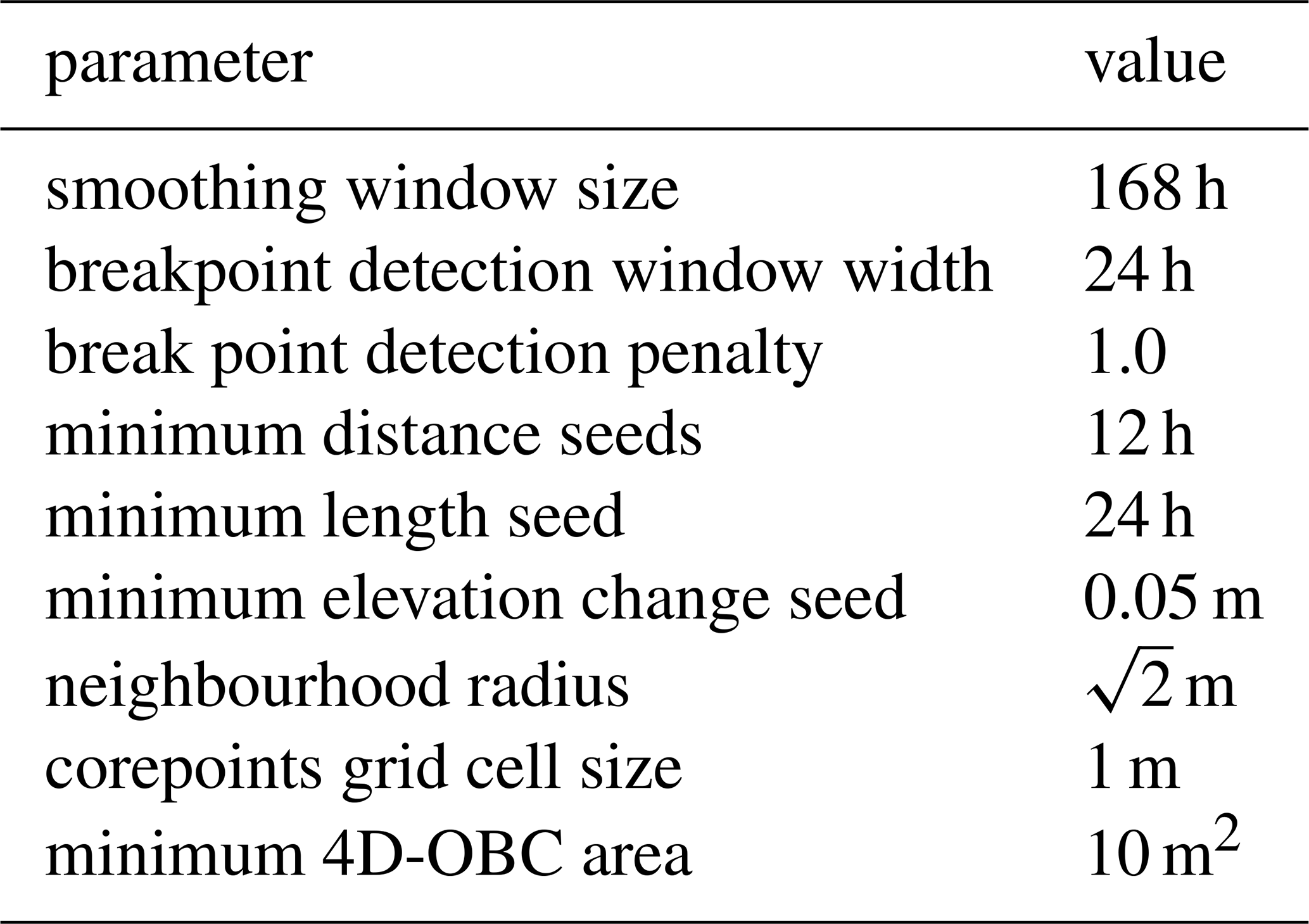
The full parameter configuration (Table 1) of the 4D-OBC algorithm is largely based on settings used in previous work on a PLS dataset at Kijkduin in the Netherlands (Anders et al., 2020, 2021; Vos et al., 2022).

Table 1 4D objects-by-change algorithm parameter configuration.

3.1.2 Point cloud selection and subsetting

Due to the massive amount of samples in the dataset, 21 194 point clouds after filtering, with on average over a million points, the 4D-OBC algorithm cannot be applied directly on the full time series. As such, the 4D-OBC algorithm and point cloud selection is optimized in two partitioning steps, to allow for computation on a High-Performance Computing (HPC) cluster.

The point cloud time series is partitioned in 9 temporal subsets. This partitioning is done to ensure no excessive amounts of memory are used, as each 4D-OBC application requires the full point cloud time series to be loaded in memory. The partitions are determined by temporal gaps in the data. When a gap is more than 6 d a new subset is created. This ensures the temporal smoothing does not overfit on single epochs (given the temporal smoothing window of 1 week), and no unrealistic jumps between epochs occur. The resulting subsets are separated by gaps of 11, 9, 10, 35, 13, 7, 7, and 19 d.

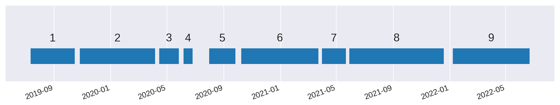
Figure 6 The temporal extent (in blue) of each subset of point clouds that are processed separately.

As 4D-OBCs are not dependent on each other between subsets, they can be computed in parallel for each subset, limiting the time needed for the computation. Figure 6 shows the date range of each subset. For each subset a low-tide point cloud is selected as reference point cloud for the space-time array computation. This subsetting has one important implication for the extraction of the 4D-OBCs, as the seeds are not transferred from one subset to the other. This means, when an elevation change after a breakpoint is not concluded, i.e., does not reach back to its initial elevation before the end of a subset, it will not be considered in the region growing and thus not become a 4D-OBC. Even though it might conclude to its initial elevation in the next subset. The subsetting strategy used here is mainly useful in cases where data gaps occur to determine obvious subset sizes. Alternative strategies could use, for example, a sliding window breakpoint detection approach or an event-based partitioning, triggered by periods of low morphodynamic activity. These could be detected with, for example, trend analysis (Kuschnerus, 2024), which would provide a more data-driven approach.

In the following partitioning step, the detected seeds per subset are divided into separate batches. These are fed sequentially to the HPC to negate its job length limitations. This subsetting has no influence on the outcome of the 4D-OBCs and has purely practical purposes. Parallel computation of seed batches is not possible, as seed selection depends on previous, already segmented objects.

The 4D-OBC extraction is performed on an HPC node equipped with 48 cores (2 × Intel Xeon E5-6248R, 3.0 GHz) and 768 GB RAM. The complete processing of all 9 subsets and their seed batches into 4D-OBCs with derived features completed in approximately 18 h of wall-clock time. The memory-intensive nature of loading a full subset point cloud time series into RAM is the primary driver for HPC use. A single subset, in our case, requires at maximum 23 GB of RAM. Parallel subset computation could thus in principle be performed on a workstation with sufficient memory, while the seed-batch step completion speed is CPU-bound and serial. Individual seed batches (of approximately 5000 seeds) take up to several hours. Using these smaller batches is found to be more efficient due to higher scheduler priority on shared HPC systems.

3.2 Step 2: processing and feature extraction

The extraction of the 4D-OBCs potentially results in a set of thousands of spatiotemporal objects representing the extent of single unordered temporary surface dynamics. The 4D-OBCs need to be further processed and characterized, to be able to group them into different types and identify recurrent 4D-OBCs. Processing of the 4D-OBCs is done by filtering the set of extracted 4D-OBCs, merging 4D-OBCs with large spatiotemporal overlap, and extracting internal features that describe the remaining 4D-OBCs.

3.2.1 Filtering of 4D objects-by-change

Some extracted 4D-OBCs have ambiguous change patterns, meaning they contain points with both erosional and depositional time series. This can occur when the magnitude of detected change is close to zero, and thus very subtle. As a consequence, a time series of opposite sign of the seed has a small DTW distance even though it is of different type. We identify these objects by computing the sign of each time series within a 4D-OBC. This sign of a time series represents net positive or net negative change, respectively erosional or depositional. It is computed by obtaining a cumulative sum of all epochs of one time series with respect to its initial elevation. The sign of the sum then determines the sign of the time series. The ratio of the two signs is used to determine if an objects is ambiguous. For our application we determine a threshold of 0.1 to be suitable for identifying most of the ambiguous 4D-OBCs, while retaining 4D-OBCs that have opposite sign for example only at the margins of the spatial segment. 4D-OBCs with a value above this threshold of 0.1 are then removed.

Further 4D-OBCs are removed that contain unnatural outlying elevation change, due to a lack of data and consequent overfit on outliers when constructing the space-time array. This is mainly occurring in the far intertidal area, where only during low-tide and small wave run-up, measurements are taken. Therefore, the 4D-OBCs that occur beyond 250 meters from the scanner, in the intertidal area, and have an absolute elevation change of more than 1 m are removed. The distance from the scanner is based on manual approximation of the average intertidal area extent. The value of 1 m is chosen as the inspected intertidal bar deposits in the dataset did not exceed this value. These intertidal bar deposits are deemed to be the largest natural dynamics occurring in the intertidal area.

3.2.2 Merging of 4D objects-by-change

Some 4D-OBCs can overlap spatiotemporally as a consequence of gaps in the data, or inadequate adaptive thresholding (Anders et al., 2021). To mitigate this effect, Ulm et al. (2025) proposed a method to merge 4D-OBCs with spatiotemporal overlap above a certain threshold. This method is also applied here, and extended by a data-driven threshold selection. The threshold level is set by testing a range of spatial overlap and temporal overlap thresholds. The overlap is measured using the intersection over union both in space and time (sIoU and tIoU, respectively). Per combination of thresholds the resulting number of 4D-OBCs after merging is computed. We then search for the combination of thresholds where both the sIoU and tIoU, show a visual change in the trend of number of 4D-OBCs with respect to lower and higher threshold values. This is comparable to the elbow method (Thorndike, 1953), which is often used for selecting the number of clusters for unsupervised clustering.

3.2.3 Feature extraction of 4D objects-by-change

To perform unsupervised clustering of surface dynamics, eight features to characterize 4D-OBCs are extracted (Table 2). These features are of spatial and temporal nature, and derived from the spatial outline and time series of each 4D-OBC. These eight features were selected based on prior knowledge of the processes that we aim to distinguish and are chosen such that they describe the varying dimensions in which these differ. All features are visualised in Fig. 7.

Table 2 Features used in unsupervised clustering of 4D objects-by-change (4D-OBCs).

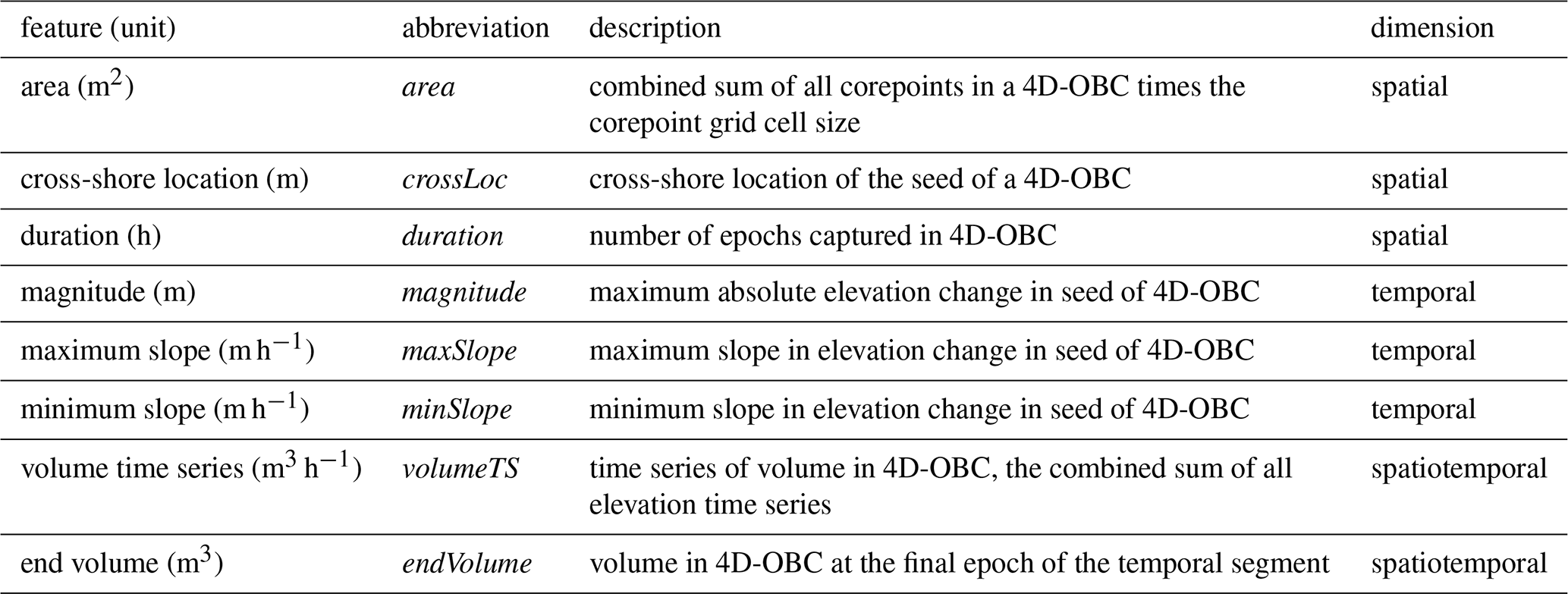
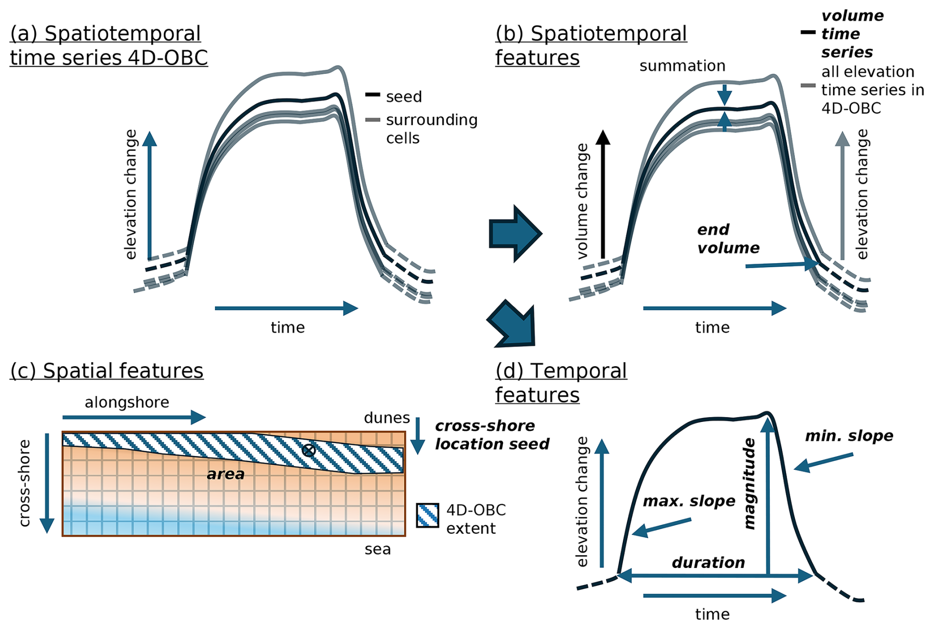
Figure 7 Schematic of features derived from the 4D objects-by-change (4D-OBC). The spatiotemporal time series (a) includes all the elevation change time series that are incorporated in the spatial segment of the 4D-OBC (c). The eight features used in this study are in italicized bold.

The spatial features are: the area (in m²) and cross-shore location (crossLoc, in m). The area is considered as the number of grid cells in the final outline after region growing. The crossLoc is considered as the cross-shore location of the seed of each 4D-OBC, measured with respect to the scanner.

The temporal features considered are duration (in h), maximum absolute elevation (magnitude, in m), maximum slope (maxSlope, in m h⁻¹), and minimum slope (minSlope, in m h⁻¹). The first is the difference in hours between the end and the start of a 4D-OBC. The second is taken as the maximum absolute elevation difference with respect to the initial elevation of the seed of the 4D-OBC. The third and fourth consider the slope as the difference in elevation of the seed between two consecutive time steps.

Two features representing combined spatial and temporal characteristics are used, the volume time series (volumeTS, in m³) and the end volume (endVolume, in m³). The volumeTS is computed for each time stamp as the sum of elevation changes over all cells in a 4D-OBC divided by the grid cell size. It thus represents the change in volume captured in a 4D-OBC over time. The endVolume is the summed elevation of all the grid cells at the end epoch of a 4D-OBC, which represents the net volume change captured in one 4D-OBC.

The volume time series (volumeTS) of individual 4D-OBCs differ in length because their durations vary. Consequently, to enable distance computation in the clustering step, all volumeTS are resampled to a common length N (the average duration across all 4D-OBCs) using linear interpolation. As a result, the volumeTS contributes N dimensions to the feature vector, whereas the remaining scalar features (duration, magnitude, etc.) each contribute only one dimension. All features are scaled from 0 to 1 using min–max normalisation to ensure equal weighting across features of different units:

$$\begin{array}{}\text{(1)}& X_{\mathrm{scaled}}={\displaystyle \frac{X-X_{min}}{X_{max}-X_{min}}},\end{array}$$

where X is the feature value of the sample under consideration, X_scaled is the scaled version of the feature value, and X_min and X_max are, respectively, the minimum and maximum feature value in the dataset.

For the resampled volume time series, X_max and X_min are taken as the largest and smallest values in all 4D-OBCs with respect to all epochs. This ensures the shape of the time series is retained after scaling. Additionally, to prevent the volumeTS from dominating the distance computation only through its higher dimensionality, all other features are multiplied by N after scaling, so that the complete volumeTS features contributes the same as one scalar feature (e.g., duration) during clustering.

3.3 Step 3: clustering of 4D objects-by-change

The set of 4D-OBCs is clustered based on the previously extracted internal features to obtain distinct groups of dynamics of which the characteristics can be analysed. This is done in three steps to allow for the analysis of surface dynamics of different levels of detail, e.g., low-level analysis of intertidal vs. backshore dynamics, and high-level analysis of different types of backshore dynamics. The dataset is first split into erosional and depositional 4D-OBCs, based on the sign of the seed elevation time series of each 4D-OBC. These depositional 4D-OBCs are thus characterised by an initial increase in elevation, and a consecutive decrease, i.e., temporary deposits; vice versa for the erosional 4D-OBCs. In the rest of this paper we refer to them as depositional or erosional objects, respectively, even though they both contain a depositional and an erosional component. The second step projects the 4D-OBCs into a detailed 2-dimensional lattice using a Self-organizing Map (SOM; Kohonen, 1990), following the approach by Hulskemper et al. (2022). The third step then clusters the nodes of this lattice at different hierarchy levels using hierarchical clustering. This combination of methods provides a balance between overfitting on outliers and overfitting on frequent dynamics.

SOMs are chosen because they provide a largely topology-preserving projection of high-dimensional data onto a 2D lattice, making inter-sample similarity visually inspectable without requiring a prior definition of the number of clusters. This is particularly suited to our dataset where surface dynamics form a continuum of types depending on research focus rather than discrete natural classes. Hierarchical clustering is subsequently applied to SOM nodes because it allows cluster boundaries to be explored at multiple levels, which makes them especially useful in the scale-dependent coastal setting, where different research questions call for different levels of morphodynamic detail to be explored.

3.3.1 Initial high level-of-detail clustering using a Self-organizing Map

We input the set of 4D-OBCs into a SOM algorithm, to obtain a 2-dimensional lattice of organized 4D-OBCs, where each cell in the lattice is representative of a specific type of dynamic, and proximal cells represent more similar dynamics. To achieve this organization, the 8-dimensional 4D-OBCs (8 derived features, Sect. 3.2.3) are iteratively mapped to a grid with at each grid location a receptive neuron with a weight vector of a similar length of 8, i.e., number of features (v_j, with j=1, …, M, M = No. grid points). All 4D-OBCs (x_i, with i=1, …, n, n = No. 4D-OBCs) are sequentially and in fixed order matched over a number of training cycles (t=1, …, T) to the closest neuron in feature space. As the SOM algorithm is a greedy algorithm, the order of training influences the resulting SOM. Therefore, we use an input order based on maximum dissimilarity sampling (Kennard and Stone, 1969), defined by the Euclidean distance between the samples. This ensures that the most dissimilar 4D-OBCs are matched first, and thus get the most weight in training, resulting in a SOM that has a greater representation of the full feature space of 4D-OBCs and is less dominated by overabundant but similar 4D-OBCs (Hulskemper et al., 2022). At every match, the weights of the receptive neuron and its surrounding neurons are updated based on the feature vectors of the matched 4D-OBC and a two-dimensional kernel. This is summarized in the following steps:

1. Initialize weight vectors, v_j with j=1, …, M

2. Select for sample x_i the closest weight vector v_i in feature space

3. Update all weight vectors based on a kernel function:

   $$\begin{array}{}\text{(2)}& {\mathit{v}}_j={\mathit{v}}_j+{\mathit{\alpha }}_t{h}_{i,j}\left(t\right)({\mathit{x}}_i-{\mathit{v}}_j)\end{array}$$

   here h_i,j is a Gaussian kernel that determines the influence of the sample x_i on all weight vectors:

   $$\begin{array}{}\text{(3)}& h_{i,j}\left(t\right)=e^{\frac{-d_{i,j}^{\mathrm{2}}}{\mathrm{2}{\mathit{\sigma }}_t^{\mathrm{2}}}}\end{array}$$

   where d_i,j is the grid distance between v_j and v_i, in grid units; σ_t is the standard deviation of the Gaussian kernel at cycle t, indicating the radius of influence of the sample; and α_t is the learning rate at cycle t.

4. Repeat step 2 and 3 for every sample in the dataset

5. Repeat step 4 for a given amount of cycles T

The closest weight vector is determined based on the Manhattan (i.e. rectilinear) distance. This is to ensure the volume time series (volumeTS, Table 2) feature, which has a different scale (Sect. 3.2.3), gets a similar weight in the distance computation as the other singular features. The initial values of α_t and σ_t are predefined and decrease with the number of cycles to achieve convergence and global and local data ordering. The values at cycle t are computed using an asymptotic decay function, with an initial learning rate (t₀) of 1.0:

$$\begin{array}{}\text{(4)}& ({\mathit{\alpha }}_t,{\mathit{\sigma }}_t)=({\mathit{\alpha }}_{t-\mathrm{1}},{\mathit{\sigma }}_{t-\mathrm{1}}){\displaystyle \frac{\mathrm{1}}{\mathrm{1}+\frac{\mathrm{2}t}{T}}}\end{array}$$

The SOM is initialised as an 8 by 8 hexagonally linked grid of randomly initialized weight vectors, with an initial kernel standard deviation (σ₀) of half of the SOM to ensure global optimum convergence (Kohonen, 1995). The SOM lattice size is chosen to provide sufficient resolution to distinguish between sub-types of dynamics within the intertidal, berm, and backshore zones, while keeping the number of nodes visually interpretable. A larger lattice could be beneficial for longer time series with a large diversity in surface dynamics. The SOM is trained for 20 000 cycles to ensure convergence. After the training cycles, all samples in the dataset are again matched to the SOM to obtain the final grouping of 4D-OBCs in SOM nodes. This grouping minimizes the variance between the final weight vectors and feature vectors of the data samples in each group, while preserving the topological relations of the data as much as possible. The SOM algorithm is applied using the MiniSOM library (Vettigli, 2018).

3.3.2 Secondary low level-of-detail hierarchical clustering

The mean feature vectors of the 4D-OBCs in every of the 2 × 64 SOM nodes are clustered in low-level clusters using an agglomerative hierarchical clustering algorithm (see, e.g., Murtagh and Contreras, 2012), implemented in scikit-learn (Pedregosa et al., 2011). Through this clustering we identify regions of the SOM that represent more comparable types of surface dynamics. The algorithm works as follows. First, the mean feature vector is computed for each SOM node. Every node is initially part of a separate hierarchical cluster. The intercluster distance of these is quantified by computing the Manhattan distances between the mean feature vectors (i.e., using average linkage). Then, with an iteratively increasing distance threshold, all nodes are merged into the cluster where the distance between the average of the nodes already inside of the cluster and the node outside is smaller than the threshold.

For a chosen distance threshold one then obtains a set of clustered SOM nodes. The chosen threshold at which we derive the clusters is based on the mean silhouette score of the clusters, computed as follows:

$$\begin{array}{}\text{(5)}& s_{\mathrm{sil}}={\displaystyle \frac{\mathrm{1}}{n}}\sum _{i=\mathrm{1}}^n{\displaystyle \frac{d({\mathit{x}}_i,\mathrm{inter})-d({\mathit{x}}_i,\mathrm{intra})}{max\left(d({\mathit{x}}_i,\mathrm{inter}),d({\mathit{x}}_i,\mathrm{intra})\right)}}\end{array}$$

where x_i is the mean feature vector of a node in a cluster, d(x_i,intra) is the mean feature distance between one node and all other nodes in the cluster it is assigned to, and d(x_i,inter) is the mean distance between the node and all the nodes belonging to the closest cluster it is not assigned to. Thus, a value of 1 indicates a perfect separation between clusters with little intra-cluster variance, whereas a value of 0 implies overlapping clusters.

The choice for a threshold is based on finding a local optimum of the silhouette score in the S_sil vs. distance threshold function. A local optimum indicates that with a small increase in threshold no clusters are formed with a greater balance between the inter and intra cluster distance, i.e., SOM nodes are added to clusters that considerably alter the current mean feature of the clusters. This local optimum can thus indicate that the cluster level at the respective threshold holds a physical value. In other environmental settings, the value of a distance threshold at which the clustering is useful can be different, depending on the dataset size and the diversity of dynamics. The silhouette-based threshold selection provides a data-driven means to adapt this threshold accordingly.

3.4 Step 4: time series and environmental analysis

The conditions and temporal patterns of the surface dynamics in the identified clusters are analysed using the active count time series of 4D-OBCs per cluster. The active count at a given epoch is defined as the number of 4D-OBCs that have started before that epoch but have not yet completed. By computing this separately per cluster, we can compare the temporal activity of different surface dynamic types. The active count serves as a proxy for process energy: a higher count implies that more sand transport events of that type are simultaneously ongoing, which can be related to the prevailing environmental conditions. It does not, however, quantify the absolute volume of sand transported, which would require integration of the volumeTS across all active 4D-OBCs.

3.5 Evaluation strategy

To evaluate the applicability of the workflow for the extraction and grouping of short-term surface dynamics occurring at different moments in time, the output of Step 3 of the workflow (Sect. 3.3) is evaluated in two ways. We investigate the feature distributions of a selection of the obtained clusters and assess their separation and coherence manually, and using the silhouette score (S_sil, Eq. 5). Furthermore, for one of the clusters the set of 4D-OBCs grouped in the cluster are investigated manually, to benchmark if these indeed appear similar, and can be interpreted as a similar type of surface dynamics. A single cluster that represents berm deposition is selected for this detailed illustration, because berm deposition is one of the most recognisable morphodynamic processes at the study site, providing a clear basis to evaluate whether the grouped 4D-OBCs represent similar type of events. Finally, we assess the variation in the appearance of different groups of surface dynamics, by computing their relative frequency per season. This is computed as the fraction of 4D-OBCs assigned to a given SOM node that were initiated during a particular season, normalised by the total number of 4D-OBCs initiated in that node across all seasons. In practice, the spatial characteristics and time series of multiple clusters were inspected by the authors to assess physical coherence; these broader checks inform the interpretation of all eight clusters presented in the results.

To assess the usefulness of the workflow for linking activity of different surface dynamics to environmental dynamics, the active count time series (Step 4, Sect. 3.4) is assessed. We notably investigate the changes in activity of a set of clusters in relation to a particular sequence of environmental conditions, here in winter 2019/2020. We focus on identifying whether variations in the activity of different groups can be related to known physical processes that lead to sand transport on beaches. We investigate to what extent certain thresholds in wave height, and extended phases of specific wave conditions, like increased wave period, can trigger changes in activity of intertidal and lower backshore dynamics; and if certain variations of wind speed and direction lead to triggering of specific activity of surface dynamics present on the backshore. Finding and interpreting such triggers and conditions within established conceptual models would indicate that the grouping is indeed physically valid, and could be used for obtaining specific insight in the conditions of selected types of surface dynamics.

4 Results

In this section we demonstrate the ability of the workflow to extract, group and link short-term surface dynamics to environmental variables from a PLS dataset of a sandy coastal setting. After extraction of the 4D objects-by-change (4D-OBCs) and processing (step 1 and 2 of the workflow, Sect. 3.1 and 3.2), we obtain a set of 4412 4D-OBCs, of which 2258 are erosional, and 2154 depositional. These surface dynamics are grouped in 2 × 64 nodes of a Self-organizing Map (SOM) and hierarchically clustered (Step 3, Sect. 3.3) to identify similar dynamics at different moments in time, characterised in terms of their internal features, like cross-shore location, duration, and magnitude (Table 2). We interpret and assess the validity of the SOM and eight selected clusters from subsequent hierarchical clustering (Sect. 4.1, following Sect. 3.5). We further assess their seasonal variations (Sect. 4.3) and variations over time compared with environmental dynamics that are known drivers of surface dynamics on the sandy beach (Sect. 4.4).

4.1 Detailed surface dynamics groups from Self-organizing Maps

The initial grouping using a Self-organizing Map (SOM) results in two lattices, one for erosional (E-SOM, Fig. 8a) and one for the depositional 4D-OBCs (D-SOM, Fig. 8b) that present the distribution of features (Table 2) among the dataset. We create lattices of 8 by 8 nodes, thus 64 nodes in total, that are hexagonally linked. Figure 8a and b show the distribution of the cross-shore location and volume change time series shape for, respectively, the depositional and erosional 4D-OBCs in the dataset.

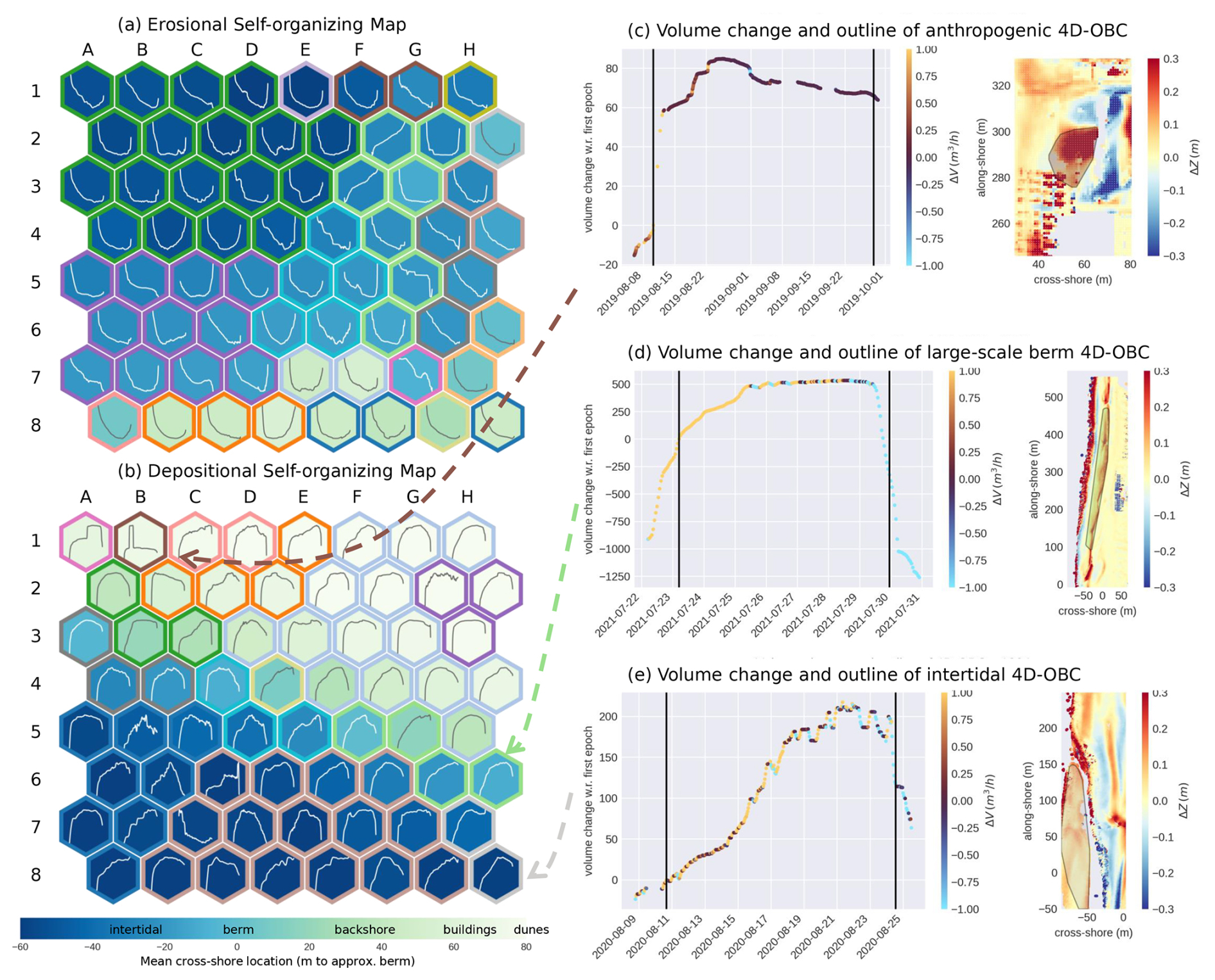
Figure 8 Self-organizing Maps (SOMs) trained on (a) the set of erosional 4D-objects-by-change (4D-OBCs), and (b) the depositional 4D-OBCs. Every hexagon is a node of the SOM and represents a group of 4D-OBCs. The facecolor is the mean cross-shore location (crossLoc, Table 2) of all 4D-OBCs matched to this node. The plot on each shows the volume time series (volumeTS, Table 2) shape of the same 4D-OBCs. The edge colours represent the hierarchical cluster in which the SOM nodes are grouped. Corresponding edge colours between panels (a) and (b) do not imply similar clusters, only similar colours within each imply similar clusters. c,d,e) show example 4D-OBCs grouped in three clusters, with their volume change time series and spatial outline as convex hull.

Through the SOM we can identify how these features vary over the set of 4D-OBCs, and thus present characteristics of the different surface dynamics they represent. The cross-shore location showcases a great ability to distinguish the 4D-OBCs into a global feature variation. Clearly, the erosional and depositional 4D-OBCs can be distinguished by their location in the intertidal area, berm, or backshore. Additionally, one can identify that the area of the SOM describing backshore 4D-OBCs is smaller for the erosional dynamics (nodes of column A–H, row 8, in Fig. 8a) than for the depositional dynamics (nodes of column A–H, row 1–4 in Fig. 8b). This can imply two things, namely, the diversity in the erosional dataset in terms of the applied features is less, or the erosional set of 4D-OBCs is more dominated by intertidal and berm activities than the depositional set.

On a local scale, so both in intertidal, berm and backshore locations, a sorting can be identified based on the slope of the growth and decay phase of 4D-OBCs. For example, the D-SOM showcases a set of abrupt 4D-OBCs on the far landward beach (e.g., nodes C1 and D1), whereas slightly more seaward on the berm, more nodes with gradual growth of 4D-OBCs are visible (e.g., nodes F5 and G5). This variation in slope of the deposition might be linked to variations in underlying processes driving the dynamics. These maps thus allow us to investigate distributions of features and shapes of dynamics captured by the 4D-OBCs.

Some nodes are very similar, and only differ slightly in, for example, their time series shape (compare Fig. 8a node A1 and B1). As such, to go beyond the study of global feature distributions of dynamics, and further study particular types of dynamics like e.g., berm deposits or bulldozer effects, further grouping of these detailed nodes is required. The SOM nodes are grouped using hierarchical clustering (Sect. 3.3.2), with a distance threshold of 0.26, and 0.3, for the erosional and depositional SOMs, respectively. This leads to silhouette scores of 0.23 and 0.24, following Sect. 3.3.2. For each SOM (Fig. 8), the colour of the outline of a node indicates a separate cluster. Similar colours in Fig. 8a and b do not imply similarity between erosional and depositional clusters, they are independent. A Principal Component Analysis (PCA) projection of the 4D-OBC feature space and SOM node positions is provided in Appendix A (Figs. A1 and A2), illustrating the distribution of 4D-OBCs and SOM nodes across the two principal dimensions of feature variation for depositional and erosional dynamics, respectively. Dendrograms of the hierarchical clustering are also provided in Appendix A (Figs. A3 and A4), showing the distances at which SOM nodes are merged and the relative separation of the identified clusters.

4.2 Broad surface dynamics clusters

From the 2 × 64 SOM nodes, 14 depositional and 17 erosional clusters are identified. From each of these sets, we further investigate four selected clusters, which are interpreted based on their feature characteristics. Figures 9 and 10, display the distribution of five selected features for these eight clusters. The colours correspond to the colours in the respective SOM. The four erosional clusters show a clear separation based on their cross-shore location (crossLoc) and magnitude, and can thus be interpreted as far and deep intertidal (cluster E8), shallow intertidal (cluster E7), and two types of backshore erosion with different magnitudes (cluster E2 and 0). The far and shallow intertidal erosion clusters are comparable in their duration, which is on average shorter than two weeks (Fig. 9b). However, they are well distinguishable by their difference in area, magnitude, and and minimum slope (minSlope, Fig. 9c, d and e). Namely the far intertidal dynamics are smaller in area, potentially due to more gaps in the data, and have a lower magnitude minSlope, they thus grow deeper, faster. The two types of backshore erosion cover very similar cross-shore locations, but can also be distinguished by their area, magnitude and minSlope. Namely, cluster E0 contains larger erosional dynamics (> 1000 m²), that can grow deeper over a shorter period of time than cluster D1 (Fig. 9c, d and e). More specifically, cluster E0 describes erosional dynamics that can cover the full beach width in size.

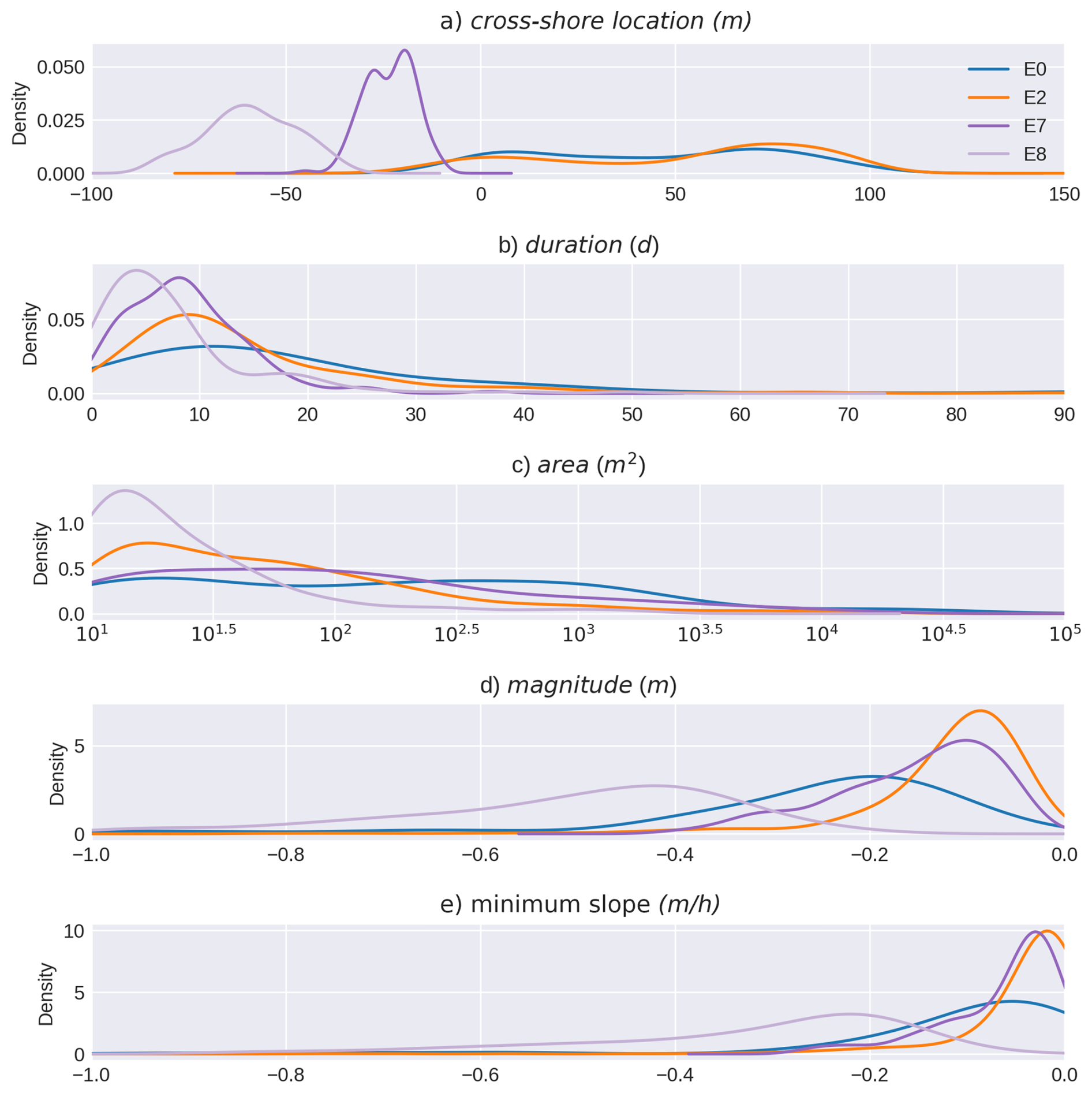
Figure 9 Density plots of five internal features of four selected hierarchical clusters (E0, E2, E7, E8) of the erosional 4D-OBC dataset. Colours correspond to the hierarchical clusters presented in Fig. 8a. The features presented are: cross-shore location of the 4D-OBCs, its duration, area, magnitude (i.e., the maximum absolute elevation change in the seed of a 4D-OBC), and the minimum slope (i.e., minimum slope in elevation change in seed of a 4D-OBC). The features refer to Table 2.

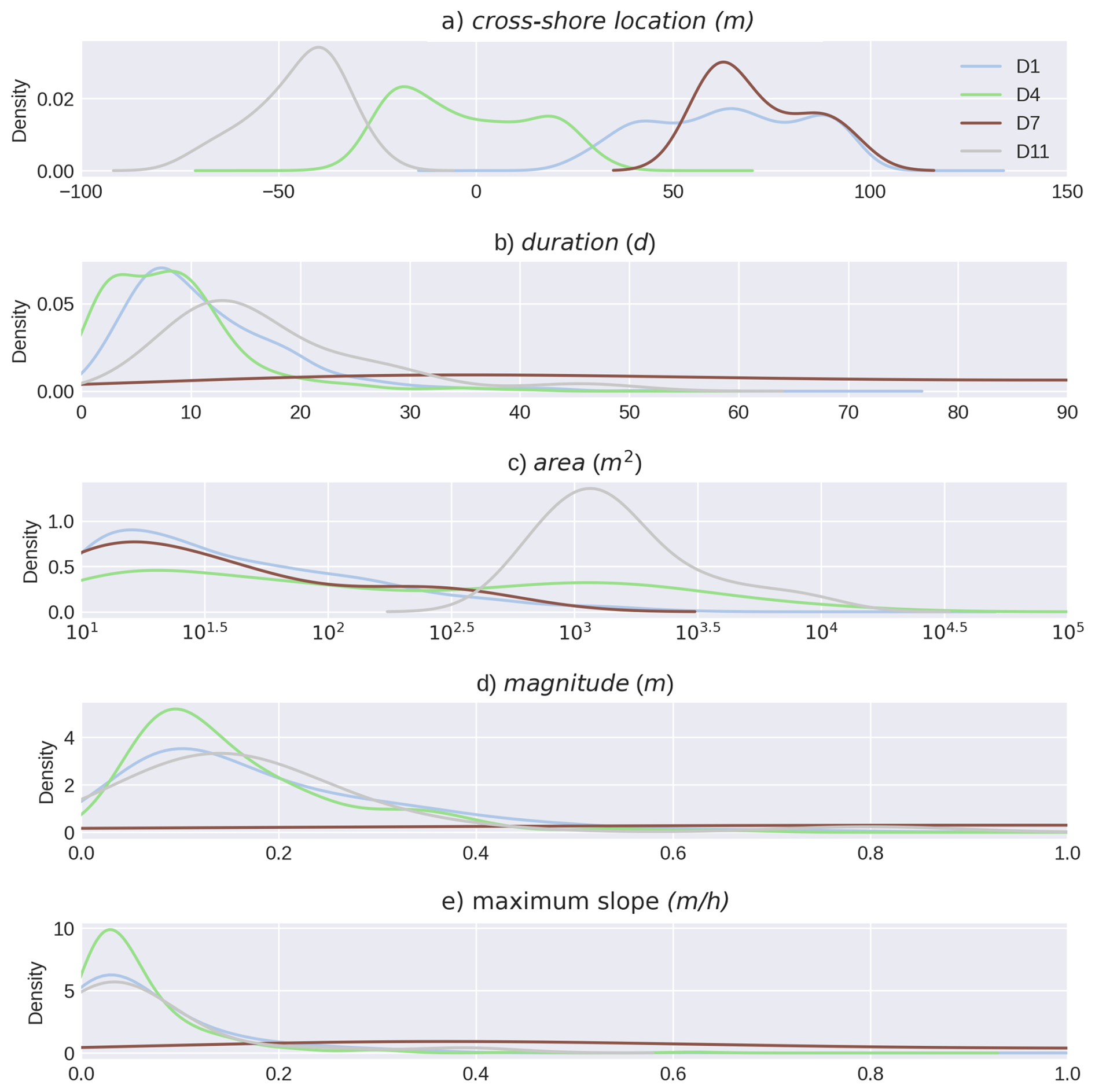
Figure 10 Density plots of five internal features of four selected hierarchical clusters of the depositional 4D-OBC dataset. Colours correspond to the hierarchical clusters presented in Fig. 8b. The features presented are: cross-shore location of the 4D-OBCs, its duration, area, magnitude (i.e., the maximum absolute elevation change in the seed of a 4D-OBC), and the maxium slope (i.e., maximum slope in elevation change in seed of a 4D-OBC). The features refer to Table 2.

The four depositional clusters also display this clear separation based on their crossLoc and magnitude (Fig. 10a and d), and can thus be interpreted as large intertidal bar deposition (cluster D11), berm deposition (cluster D4), and high magnitude (cluster D7) and low magnitude far backshore deposition (cluster D1). Further characterisation is done based on the duration, area and maximum slope (maxSlope, Fig. 10b, c and e). The intertidal bar depositions are only of a large area (around 1000 or more m²), and have a longer duration than the berm depositions (several weeks compared to one week). Figure 8c, shows an example of one of the intertidal bars of cluster D11, whereas Fig. 8b shows a large scale berm deposition of cluster D4. The latter can be interpreted as the gradual welding of a bar to the berm. The two backshore clusters are easily distinguishable by their magnitude and maxSlope, with cluster D7 being a lot higher in these regards. This high magnitude, and maxSlope might indicate dynamics that are of human origin. If we inspect the outline and time series of volume change of one of the 4D-OBCs found in this cluster (Fig. 8a), it can be seen that it is a very local change, and surrounded by areas of erosion of comparable magnitude. This suggests local sand transport by bulldozers. The large spread in duration of the 4D-OBCs in this cluster also suggests that the changes they describe are not of a nature that is easily adjusted for in a natural morphodynamic equilibrium.

Examples of 4D objects-by-change found in a single cluster

The investigated clusters have coherent feature distributions, through which the 4D-OBCs are separated in different feature dimensions. This indicates that we are able to identify similar surface dynamics at different instances. To further demonstrate this ability to group similar dynamics at different moments in time, we assess several 4D-OBCs grouped in the berm deposition cluster D4 on their appearance and timing.

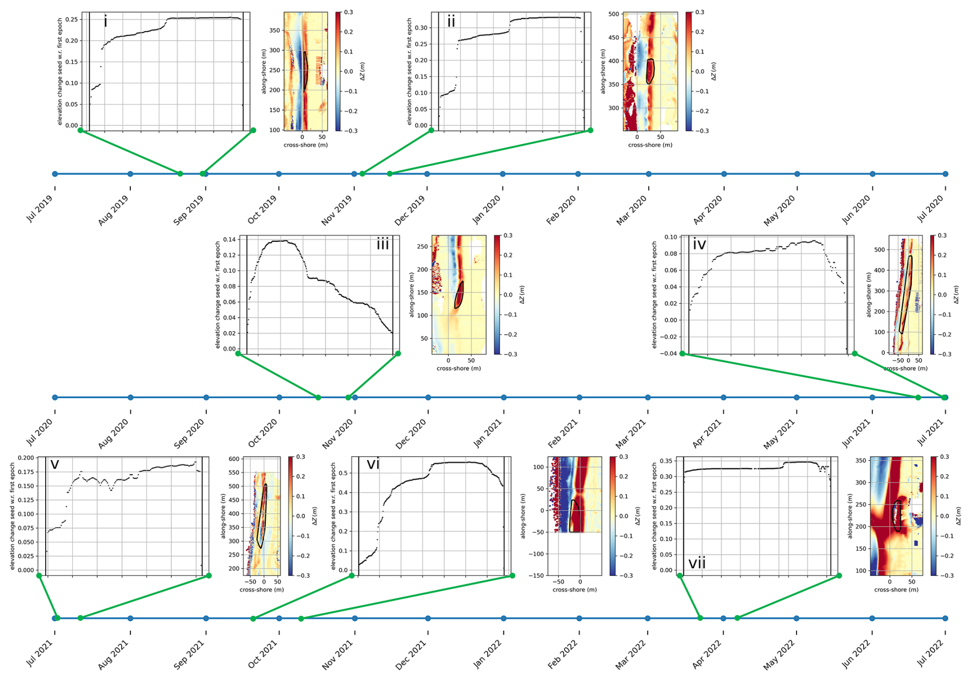
Figure 11 Timeline of the full dataset, with examples of the temporal extent of 4D objects-by-change (4D-OBCs) clustered in depositional cluster D4. The seed elevation time series and the convex hull around the spatial outline of the 4D-OBCs is visualised. The latter is drawn on top of the elevation change w.r.t. the start epoch of the 4D-OBC.

Figure 11 shows a timeline of the three years of data with the temporal extent and characteristics of seven 4D-OBCs found in cluster D4. All the 4D-OBCs are indeed located somewhere around the centre cross-shore location, some are more inland (e.g., Fig. 11ii), and some more seaward (e.g., Fig. 11i). However, all can be found around the estimated berm, and are thus likely part of a surface dynamics creating varying berm positions throughout the year. Furthermore, most of the 4D-OBCs contain a similar time series of elevation change, with a two step increase in elevation, concluded by a fast decrease (Fig. 11i, ii, v, vi, and in some respect iv). 4D-OBCs in Fig. 11iii and vii show fairly different patterns of elevation change. The latter is very instantaneous both in its increase and decrease, which might indicate anthropogenic deposition and removal. The duration of all 4D-OBCs is quite comparable, with a period of up to two weeks. The length in alongshore direction, however, is different, where some are very long (iv, 400 m), and others are short (ii, 50 m) but seem to be part of a elongated long-shore section of deposition with interruptions (also iii an vi). Figure 11vi, in particular, does not yet appear to have fully developed across the entire spatial extent of the surface dynamic.

4.3 Seasonal variations in activity of surface dynamics

Following the extraction and interpretation of different types of short-term surface dynamics based on the internal characteristics of the 4D-OBCs, we can now investigate if and how these groups exhibit variation in their temporal occurrence over the years. Figures 12 and 13 display the relative occurrence of 4D-OBCs in different SOM nodes (Sect. 3.3.1) in the four seasons computed over the three-year dataset.

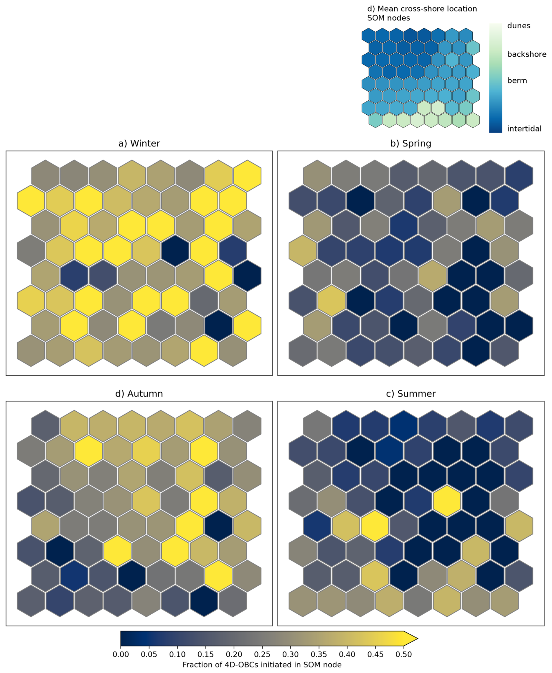
Figure 12 Fraction of the number of 4D objects-by-change (4D-OBCs) initiated in the different seasons for every Self-organizing Map (SOM) node in the erosion SOM. The seasons refer to the Northern Hemisphere seasons: Winter (December–February), Spring (March–May), Summer (June–August), Autumn (September–November). (d) The average cross-shore location of the 4D-OBC in each node.

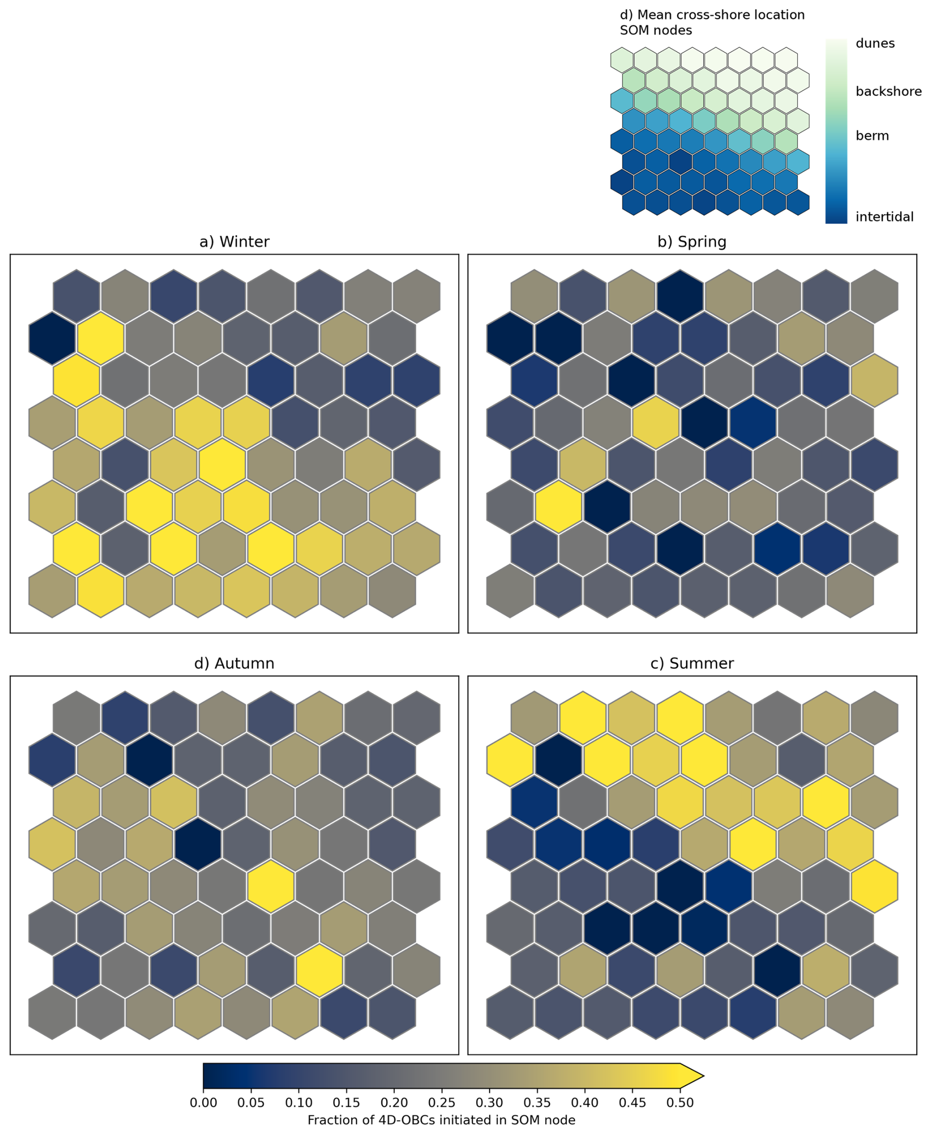
Figure 13 Fraction of the number of 4D objects-by-change (4D-OBCs) initiated in different seasons for every Self-organizing Map (SOM) node in the deposition SOM. The seasons refer to the Northern Hemisphere seasons: Winter (December–February), Spring (March–May), Summer (June–August), Autumn (September–November). (d) The average cross-shore location of the 4D-OBC in each node.

Figure 12 clearly shows varying activity of different types of dynamics in different seasons. In winter, 4D-OBCs occur over the whole SOM space with few exceptions, whereas in spring only relatively few 4D-OBC are active. In summer and autumn, the activity is unevenly distributed. In summer, the erosional dynamics that occur are found mainly at the bottom of the SOM. These nodes correspond to 4D-OBCs on the backshore (Fig. 12d). In autumn, on the other hand, the active nodes are mainly at the top right of the SOM, corresponding to 4D-OBCs located in the intertidal zone. However, other nodes representing intertidal surface dynamics are not as active (lower left of the SOM). This indicates that different types of intertidal dynamics are active in different seasons.

Figure 13 displays a comparable pattern of seasonal variations, where the main difference is the lack of depositional activity in the top right of the SOM in winter. This corresponds to the area of the SOM with 4D-OBCs of the backshore (Fig. 8b). Thus, little deposition on the backshore takes place in the winter. Whereas in summer most of the backshore depositional dynamics occur, and only relatively little intertidal depositional 4D-OBCs (lower left in Fig. 8b).

These results show that particular seasons are dominated by both erosional and depositional surface dynamics. This indicates that in these seasons erosional and depositional dynamics coexist in different parts of the beach, or that they appear in periodic sequences throughout a season. Further investigation of a sequence of surface dynamics activity might demonstrate this.

4.4 Sequence of activity of surface dynamics during winter 2019/2020

To further demonstrate the applicability of the workflow for studying characteristics of short-term surface dynamics, we compare the variation in active count time series of the eight interpreted clusters (Sect. 4.1) to variations in environmental variables, as described in Sect. 3.5. We do this on a detailed scale by zooming in on a five month period of activity in the selected clusters between November 2019 and April 2020 (Fig. 14).

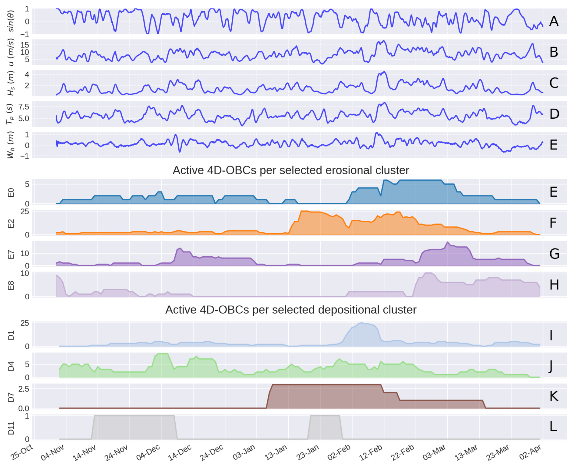
Figure 14 Five-month time series in 2019/2020, of 24 h moving averaged environmental dynamics, with (A) sine of wind direction w.r.t. the coast, (B) wind speed, (C) wave height, (D) wave period, provided in Appendix A water level. The active number of 4D objects-by-change (4D-OBCs) of the selected erosional clusters (EFGH) of Fig. 9 and depositional clusters (IJKL) of Fig. 10. All colours refer to the same colours as in Fig. 8.

In the top five panels the environmental dynamics are plotted. Here we take the 24 h rolling mean for better interpretability. Figure 14A, B, C, D, and E display the sine of the wind direction (Sect. 2.2), wind speed, significant wave height, wave period, and water level, respectively.

4.4.1 Variations in erosional (E0 and E2) and depositional (D1 and D7) backshore surface dynamics

The two backshore erosional surface dynamics clusters show similar low amount of activity until mid January, whereafter activity of cluster E2 increases to 25 active 4D-OBCs within days. These days are characterized by seaward windspeeds around 10 m s⁻¹. Indeed, the lack of fetch length from this direction can cause the erosive potential to be large on the beach.

However, the larger scale erosional cluster (cluster E0) only notably activates later, at the beginning of February. At this time, the predominant wind direction is slightly shifted towards a more along-shore direction, which should increase the fetch length and thus, contradictory to what the results indicate here, lower the erosive potential and activity. Indeed, at this time we also observe a peak of depositional activity of the backshore, with activation in depositional cluster D1. The question is how these can coincide. Comparing the location of cluster E0 in Fig. 9a, and cluster D1 in Fig. 10a, we identify that cluster D1 is more confined to the far backshore area, whereas cluster E0 also occurs on the seaward side of the backshore.

This peak in both cluster E0, and cluster D1 under alongshore high windspeeds, increased stable wave heights, period, and water level could then conceptually be explained as follows. First, on the seaward part of the backshore, the wave run-up reached far for a longer period of time under this increased water level and wave height, forcing large scale hydrodynamically driven erosion (activity in cluster E0). The waves however did not reach to the far backshore, but here, as a consequence of buildings and other human deployments at the beach, local sheltering and turbulence might have caused lowering of wind speeds (Poppema et al., 2021). Because this coincided with a large fetch length, alongshore wind transported sand to the far backshore, where the sand got deposited, increasing activity in cluster D1. Next, one week later, around 10 February, almost all the 4D-OBCs in cluster D1 got eroded again, whereas the erosional activity in cluster E0 and 2 increased. The doubling of the number of 4D-OBCs in cluster E0, in particular, indicates instantaneous erosion occurring all over the beach (see Fig. 9e). At this time, the wind speeds are vastly increased to above 15 m s⁻¹ whereas the direction is more landward, which results in less obstruction of wind at the far backshore, and a smaller fetch length, increasing the erosive potential all over this backshore area.

4.4.2 Variations in erosional (E7 and E8) and depositional (D4 and D11) intertidal and berm surface dynamics

The intertidal and berm depositional and erosional dynamics also show large changes in activity under varying circumstances. Over the months, two intertidal bar deposits occur (cluster D11). Both of these get initiated under wave heights of 2 m and wave periods of 6 s or higher (13 November 2019 and 20 January 2020). Then, only after wave heights reach even higher than 2, do the bars get completely eroded (9 December 2019 and 30 January 2020). Erosional intertidal dynamics (cluster E7 and 8) have two distinct peaks in activity. The first only relates to cluster E7, and occurs at the same time as the erosion of the intertidal bar of depositional cluster D11 at 9 December 2019. This coincides with a very sharp increase in wave height, period, but more notably a fast periodic variation of water level. The second peak occurs around 23 February 2020, where both cluster E7 and cluster E8 gain a sharp increase in activity, thus we see both erosion in the far and near intertidal and also of greater magnitude (compare magnitude in Fig. 9d of cluster E7 and E8). Around this time, the environmental dynamics do not necessarily experience a peak, but are rather high for a sustained period of time. The wave height is above 2 m, wave period above 6 s, and the water level remains above 0 m w.r.t. N.A.P. for around half a month, during which the activity in both groups start to peak. This indicates that the temporal duration of high-energy circumstances has great effect on the nature of the short-term dynamics of the system, be it eroding or depositing.

Depositional cluster D4 (berm depositions) shows slightly more variation with a constant presence all over the period under consideration. What is noticeable is that the activity signal appears to be following the signal of the wave period, and wave height, or a combination thereof, as is visible around the end of February. In some cases, this increase in activity occurs with some delay. For example, compare the increase in activity around 1 December 2019 to the increase in wave period and wave height around that day. Thus, with increased wave period, an increase in berm depositions occurs, but this relation does not hold in cases with only short peaks in wave height and period.

5 Discussion

This study presents a novel workflow for extracting, grouping, and interpreting short-term surface dynamics in a sandy coastal system using dense 4D topographic measurements. We demonstrate the effectiveness of combining self-organizing maps (SOMs) and hierarchical clustering to derive physically interpretable groupings of surface dynamics from a set of 4D objects-by-change (4D-OBCs). This grouping is effective even when dynamics appear at different moments in time throughout a multi-year observation period. The variations in activity of the eight selected groups are physically interpretable, and relate to changes in environmental conditions. This discussion evaluates our findings in relation to the central research question: How can short-term surface dynamics in sandy coastal systems be extracted, grouped, and linked to environmental variables?

5.1 Extraction of surface dynamics

The extraction of surface dynamics as 4D-OBCs enable the analysis of spatiotemporally coherent segments of elevation change. In previous work, these have been extracted and validated for datasets of 4D topographic measurements up to several months with around 3000 hourly epochs (Anders et al., 2020, 2021, 2022; Ulm et al., 2025). In the workflow presented here we enable the extraction of 4D-OBCs from even longer time series of hourly point clouds, where computational memory and time-constraints limit applicability, by enabling parallel computation in subsets, and serial computation in seed batches. In combination with the application of the C++ implementation of the 4D-OBC algorithm in the open-source Python library py4dgeo (Anders et al., 2026), we achieved extraction of 4D-OBCs and derivation of features from a set of 21 194 point clouds in only 18 h on an HPC (48 cores, 2 × Intel Xeon E5-6248R, 3.0 GHz, and 768 GB RAM), with subsequent clustering on a relatively small workstation within 1 h (32 GB RAM, 24 cores). This efficient processing offers the potential to further apply the methods on even larger datasets in future work, with the possibility of incorporating 4D-OBC detection on hierarchical spatiotemporal scales.

5.2 Grouping of surface dynamics

The application of the SOM on the extracted 4D-OBCs enables the unsupervised grouping of the full set of 4412 4D-OBCs based on the internal distributions of eight derived features, such as duration, cross-shore location, and magnitude of elevation change. The SOMs capture non-linear patterns in the eight-dimensional feature space and offer an intuitive layout for assessing inter-node similarities. Visualising a feature like volume time series shape, along with cross-shore location, enables the identification of patterns of characteristics in the dataset of surface dynamics. For example, the erosional dynamics show a lower diversity in or number of backshore dynamics than the depositional dynamics, indicated by the smaller apparent area of backshore dynamics in the respective SOM (Fig. 8a).

Through hierarchical clustering of SOM nodes, we identify 14 depositional and 17 erosional dynamic types. The clusters have coherence in their internal features and allow for interpretation of morphodynamic processes such as berm deposition, large-scale beach erosion, and anthropogenic activity. For example, cluster D7 can be linked to localized sand placement, likely by bulldozers, based on its high magnitude, rapid volume change, and spatial characteristics that are different to natural deposition patterns. This opens up the possibilities to study relative impacts and frequencies of anthropogenic dynamics, which have been previously found in these datasets (Kuschnerus et al., 2021), but to the best of our knowledge not studied in detail.

These findings highlight how unsupervised clustering methods applied to the 4D-OBC feature space can, for this environmental setting, extract morphodynamically meaningful patterns without the need for predefined class labels or thresholds. Which is demonstrated for the eight clusters investigated in this study. The clustering method greatly advances existent methods of PLS data analysis (Anders et al., 2020; Kuschnerus et al., 2021, 2024a), as we are now able to bring together similar 4D-OBCs, i.e. instances of surface dynamics types, occurring at different moments in time. Consequently, this enables us to study the different environmental conditions, or periods in which surface dynamics with different characteristics exist. Moreover, the grouping allows for identifying variations in location of morphodynamic zones, given by temporal cross-shore location patterns in the occurrence of specific types of dynamics. These zonations can reflect patterns of change in the extent to which hydrodynamic or meteorological forces can affect sand transport in the beach system and can thus provide a new way of analysing changes in drivers of cross-shore dynamic zonation.

The SOM provides a scalable and flexible grouping method: larger SOMs could be applied to explore more complex systems or longer datasets, with hierarchical clustering acting as a second-stage simplification step. This hierarchical structure of clustering gives a high grade of visual interpretability, and allows to identify levels of grouping which, depending on the application, can be investigated at varying hierarchies (cf. the dendrogram in Appendix A). Future work could further explore and optimize the specific settings of the SOMs and clustering. We found that, with current parameters, the E-SOM shows less diversity in the identified surface dynamics than the D-SOM (cf. Appendix A), which could be due to the erosional dynamics being more consistent over time, or their variation might be in different features than for the D-SOM. Optimizing settings for the two datasets separately instead (e.g., a smaller SOM and testing spatial shape features for erosional dynamics) might increase the representativeness of the clusters.

Future clustering applications may benefit from using density-based alternatives to hierarchical clustering such as Hierarchical Density-Based Spatial Clustering of Applications with Noise (Campello et al., 2015), which can identify clusters of varying density and flag low-density nodes as noise. This would reduce overfitting to some outlying dynamics/artefacts by not forcing them into a cluster, as occurs in our workflow. Such methods would however require alternative validation metrics suited to density-based clustering, such as the Density-Based Clustering Validation score (DBCV; Moulavi et al., 2014), instead of the silhouette score used here. Other simpler methods like k-means clustering offer another alternative but requires the number of clusters to be predefined and assumes approximately spherical, equal-variance clusters, assumptions unlikely to hold for the complex varying dynamics found here.

The application of this unsupervised classification workflow is not limited to coastal areas or specifically to 4D-OBCs. The approach is generalizable to any set of time series segments of topographic measurements, enabling the identification of similarly behaving surface dynamics at different moments in time. Adaptation may be required through additional feature engineering. For instance, in a coastal setting with lower point density data such as ICEsat line-sampled measurements (Xu et al., 2024), temporal segments of uniform change could be identified using the breakpoint detection method (Sect. 3.1) or trend fitting (Kuschnerus et al., 2024a). Features could then be extracted directly from these segments, without relying on the spatial or spatiotemporal features provided by 4D-OBC region growing. Instead, additional temporal descriptors (e.g., acceleration of elevation change) could be incorporated before applying the SOM and hierarchical clustering to group locations with similar dynamics.

In other environments, such as landslide- or avalanche-prone alpine regions (e.g., Kromer et al., 2017), the workflow could be adapted by modifying the seed detection step of the 4D-OBC method (e.g., restricting to uni-directional changes as in Anders et al., 2022). Feature design and selection would also differ, e.g., slope or acceleration of elevation change could help distinguish slow mass movements from rapid landsliding, while location-based features such as the cross-shore location used in the coastal setting would be less relevant.

5.3 Linking surface dynamics to environmental dynamics

The temporal activity of specific clusters and SOM nodes reveals known links between surface dynamics, seasonality and environmental dynamics, including wind direction, wind speed, wave height, wave period, and tidal water levels. Seasonal patterns are present in the SOM grouping, with an increase in intertidal erosion in autumn and winter, consistent with seasonal storm-driven dynamics of sandbars (Van De Lageweg et al., 2013). We can however identify specific types of intertidal erosion dynamics that are less active in autumn. Activity in both erosional and depositional clusters of intertidal dynamics coincided with wave heights exceeding 2 m and peak wave periods above 6 s, supporting previous findings on energetic thresholds for enabling changes in morphodynamic states of the beach (Wright and Short, 1984; Castelle and Masselink, 2023). Further statistical analysis could then allow for the acquisition of site or time-specific threshold conditions in which different dynamics take place.

Through investigation of the relative activity, we show that wind speed and direction, in combination with fetch and obstructions, have a complicated but strong relation to patterns of activity in backshore depositional and erosional dynamics. Small scale erosional clusters gain an increase in activity under shorter fetch conditions through a seaward wind direction, which respond most sensitively to sustained high wind speeds (> 10 m s⁻¹). In contrast, small depositional clusters on the far backshore get activated under similar windspeed, when there is an alongshore direction. Their deposition is likely the result of obstruction by buildings, creating local turbulence and lowering of wind speed. These findings support earlier research highlighting the complex interaction between fetch length, and threshold wind velocity for aeolian transport initiation and deposition (Delgado-Fernandez, 2010), and emphasize the need for considering (man-made) obstruction when predicting sand transport processes (Poppema et al., 2021).

In addition to peak event characteristics, the duration of high-energy wave conditions also influences morphodynamic response captured in the 4D-OBCs. Extended periods of elevated wave energy and water level lead to increase in intertidal erosion clusters. Moreover, variations in berm deposition can be related to sustained variations in wave period and wave height, whereas short peaks do not seem to have a similar effect on activity of berm depositions. These observations are in line with the concept of morphological relaxation time, varying periods of energetic conditions are required to drive substantial adjustments in intertidal bar systems of different scales (Masselink et al., 2006).

Future studies could include more environmental dynamics, such as wind speed variance, wave direction, precipitation, and combined multivariate dynamics, e.g., through principal component analysis or multivariate time series analysis. Moreover, quantification of thresholds for the initiation of different dynamic types, or even a statistical or causal analysis of interactions between environmental dynamics and surface dynamics could inform a data-driven way of modelling of short-term surface dynamics processes.

In particular, the found groups of surface dynamics, together with these environmental dynamics can be used to develop physics-based prediction models (Karniadakis et al., 2021) of surface dynamics that could inform coastal management. By combining observed surface dynamics and time series of environmental variables, physics informed machine learning methods could learn specific conditions linked to surface process activity, which in this study were identified manually. Through these predictive models one might then anticipate certain high-impact dynamics and possibly prepare through adequate beach management. Additionally, these short-term prediction models could be extrapolated to future climate scenarios to identify possible impact on longer-term morphodynamic projections.

5.4 Limitations and implications

The interpretation of the results highlights the inherent complexity of the coastal system. Even under seemingly similar environmental conditions, the temporal patterns in activity across clusters of surface dynamics vary considerably, suggesting that there are other, possibly unmeasured, factors influencing the response. This includes the sequence of events, the previous morphological state, sediment availability outside of the measured area, or other cumulative effects. It furthermore emphasizes self-organization in the system, as the current state affects how the system evolves, even without a clear or direct external trigger (Coco and Murray, 2007). Sediment availability from along-shore transport or the foreshore are not directly measured as potential environmental drivers in our study but assumed to be implicitly reflected in the extracted 4D-OBCs and history of environmental variables. In a future PLS setup, explicit monitoring of these boundary conditions (through e.g., regular monitoring with bathymetric sensors, wider-area UAV surveying, or acoustic sediment transport sensors), or exploration of the prediction thereof through the history of environmental variables in combination with, for example, LSTMs, could aid further explanation of identified beach dynamics and their variation.

Nonetheless, the results show that the characteristics of the grouped 4D-OBC clusters, and their temporal variations, are interpretable in terms of known coastal processes. What this method offers is not a complete explanation of morphodynamics in a PLS dataset, but rather a structured way of reducing the high dimensionality of extensive point cloud time series into types of surface dynamics. This discretization enables systematic comparisons, temporal analyses, and correlation studies, which would be otherwise infeasible. It also allows the targeted investigation of particular types of dynamics (e.g., berm growth, bar migration), and opens the door for more detailed analyses of their environmental drivers.

However, several methodological limitations remain. The current 4D-OBC definition is tied to temporary elevation change, but in practice, some dynamics have a net change (i.e., volume gain or loss, e.g., Fig. 8a node 2F). This may result from the inclusion of growing regions with only partial similarity during part of the dynamic, leading to incomplete closure of the object. As we cluster on these volume features, these types of 4D-OBCs can be distinguished afterward, and thus separately analysed and regarded. However, it is a particularity of the 4D-OBCs that does influence its applicability on studies of volume change. One possible refinement would be to define unidirectional or partial dynamics (e.g., only build-up or erosion) like previous methods (Anders et al., 2022; Kuschnerus et al., 2024a). Spatially splitting objects into separate positive or negative parts might support this, e.g., by filtering individual 4D-OBCs at their spatial margins after or during region growing through testing whether added corepoints show a coherent direction of elevation change.

The current 4D-OBC filtering step, that excludes non-natural intertidal dynamics of excessive change, may in other locations exclude large but natural 4D-OBCs like sandbars under nourishments. A larger threshold may offer a better balance, but it increases the risk of outlier inclusion. Possibly, to fully avoid this step and reduce the number of outlying 4D-OBCs in the intertidal area, the point cloud time series processing could be improved upon by adding a step to filter out water points, and/or use only low-tide scans.

The choice of features influences clustering outcome, and correlated features may bias groupings. In this work the features are selected based on previous knowledge about the processes to be clustered. A data-driven feature selection, using e.g., Shapley values (Fryer et al., 2021) and a labelled dataset might increase effectiveness of the clustering. Furthermore, the way the volume time series (volumeTS, Table 2) is incorporated as a feature could be changed. Currently, we resample the time series such that they all have the same number of dimensions and a Manhattan distance can thus be computed between different 4D-OBCs. In the future the use of DTW distance instead of Manhattan distance could allow to compare the time series of different lengths directly. Or, the derivation of other time series-based features alike Wang and Anders (2025) could be used as a substitute.

The interpretation using the active count of 4D-OBCs allows us to identify the distribution of the energy of the system into different dynamics. This offers the possibility to study its variations over time and gives indications on sand redistributions over the study area. There are, however, several limitations to the extent to which these interpretations are valid. First, the active count is decreased at the start of a subset (Sect. 3.1.2), and decreases per definition when coming to the end of a subset, as fewer seeds complete their deposition-erosion cycle before the subset is ended. This decreases the interpretability of changes at the margins of a subset, which should be taken into account during analysis, in particular when statistical analysis are carried out. To add continuity across subsets and reduce edge effects, future work could use only daily low-tide scans to reduce the number of epochs, and allow single batch processing, or develop a mechanism to transfer non-concluded seeds across subsets.

Furthermore, the use of a time series of volume within 4D-OBCs of different types of dynamics, instead of an active count time series could in future work be investigated. As this would actually quantify sand redistribution on the beach, and would thus be preferable for analysing sand redistribution through different surface dynamics. However, the current design of te 4D-OBC segmentation method does not allow for this. As follows from the results (e.g., object vi in Fig. 11), not all 4D-OBCs fully delineate the extent of a surface dynamic, either because a surface dynamic lies partially outside of the data coverage, or because the outer areas of the surface dynamic are too different from the internal area of the seed. If a correct measure of volume inside types of dynamics is wanted, these partial 4D-OBCs should be detected and flagged, or their growth must be optimised. Additionally, for these volumetric redistribution studies the addition of the dunefoot, dune and subtidal area in the topographical data would be preferred. This would require either a higher position of the LiDAR sensor, to diminish occlusion, or the incorporation of additional LiDAR sensors targeting the dunefoot. Incorporating sand redistribution in the dune area would also require effective separation of vegetation and sand through point-wise classification methods.

The reliance on unsupervised clustering avoids the need to predefine surface dynamic classes, which is an important advantage in a natural coastal system where class boundaries are continuous and scale-dependent. This, however, means we require manual validation, and there is no quantified external validation against labelled ground truth. This makes it difficult to assess whether a given parameterisation is optimal or to compare methods extensively. In future work, development of benchmark datasets of labelled 4D-OBCs, derived using video imagery or expert annotation of known events, could enable quantitative validation, data-driven feature selection, and consequently greater confidence in the transferability of the workflow to new sites.

A limitation of the environmental analysis is the use of monitoring stations located up to 35 km from the PLS site. While the large-scale spatial coherence of wind and wave conditions along this coast justifies this for our scale of analysis, local effects and subdaily temporal variations will not be fully captured. For future data-driven correlation and prediction studies, locally measured or spatially interpolated/downscaled environmental variables would be worth investigating.

6 Conclusions

In this paper, we present a workflow to extract and group similar short-term topographical surface dynamics independent of their timing, from large 4D permanent laser scanning (PLS) datasets of sandy coastal topography. This is done through unsupervised and automated classification of 4D objects-by-change (4D-OBCs; Anders et al., 2021). We first refine the application of the 4D-OBC method to effectively process three years of hourly data, totalling 21 194 point clouds. These 4D-OBCs are further processed to extract eight internal features that characterise the 4D-OBCs as surface dynamics. Then, the 4D-OBCs are grouped into different types of surface dynamics at two levels of detail using Self-organizing Maps (SOMs) and subsequent hierarchical clustering.

We demonstrate that through the workflow we obtain clusters of 4D-OBCs that reveal coherent feature distribution which are physically interpretable as different types of surface dynamics, like berm deposits, high magnitude anthropogenic deposits, or large-scale beach erosion. 4D-OBCs in a single cluster are manually interpreted and indeed yield 4D-OBCs of similar appearance at different moments in time throughout the three years of hourly data. Broader inspection of feature distributions of a further eight clusters supports this coherence of surface dynamics type. Consequently, we demonstrate the ability to identify if a surface dynamic with a certain set of characteristics appears at different moments in time.

The fact that the method can bring together similar surface dynamics independent on their relative timing, allows for the analysis of the internal, seasonal and environmental characteristics of types of short-term surface dynamics. Zonation of specific types of dynamics, e.g., the cross-shore variation in berm location throughout the years can be identified. Additionally, seasonal variations in the presence of certain surface dynamics can be uncovered through the SOM, which show logical relation to known seasonality in sandy beach surface dynamics. Furthermore, we demonstrate that the surface dynamics can be related to environmental variables by assessing the variation in number of active 4D-OBCs per cluster.

In future work, the developed workflow can be used in more focused studies to identify threshold conditions and correlations between (combinations of) environmental drivers and initiation of different types of surface dynamics. Time series representing the activity of these surface dynamics can be used as output of generative machine learning models, where the inputs are environmental dynamics. If effective, these predictions can then help inform effective coastal management by anticipating high impact events, and through extrapolation assess how specific short-term changes interplay with longer-term morphodynamic trends.

Appendix A: Visualisation of 4D-OBC, SOM and hierarchical clustering space

In Figs. A1 and A2, the 4D objects-by-change (4D-OBCs) and mean Self-organizing Map (SOM) node positions are plotted in the 2-dimensional Principal Component (PCA) space based on the feature vectors of the 4D-OBCs. It can be seen that for the Deposition SOM (D-SOM, Fig. A1), the mean feature vectors of the various hierarchical clusters and SOM nodes are well distributed over the feature space, with some outlying regions well represented (e.g., the green dots, cluster D4). The erosional SOM (E-SOM, Fig. A2), in contrast, shows less even distribution of SOM nodes over the PCA space. The SOM nodes of similar hierarchical clusters are closer together than in the D-SOM. This implies that the E-SOM does not represent the full feature space of erosional surface dynamics as well as the D-SOM. A possible reason for this could be that erosional surface dynamics show less variability in the features applied here. In future work, it could be tested if a different SOM configuration and feature engineering could result in a more even distribution of SOM nodes over the feature space.

Figures A3 and A4 show the dendrograms of the agglomerative hierarchical clustering of SOM nodes for the depositional and erosional datasets, respectively. The majority of clusters merge at relatively low distances, indicating compact and well-separated groups. A subset of nodes, particularly in the E-SOM, merge only at large distances, which possibly represent rare dynamics or data artefacts at the margins of the feature space. The chosen distance thresholds (dashed lines) correspond to local optima of the silhouette score as described in Sect. 3.3.2.

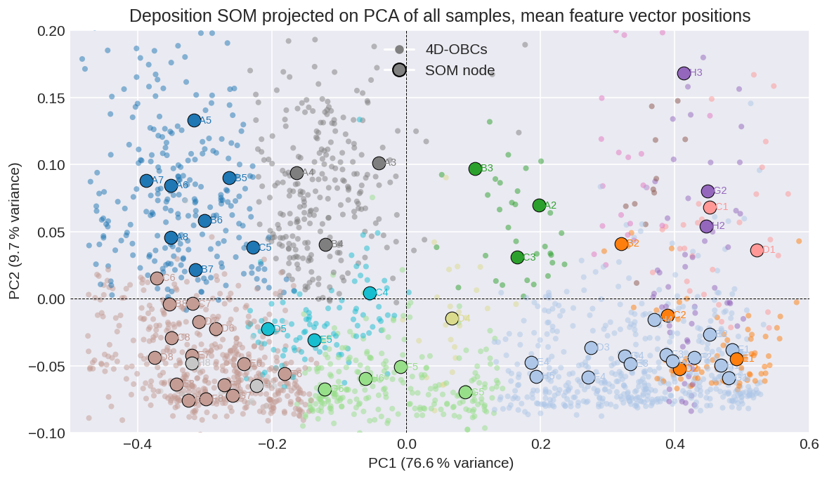
Figure A1 Space defined by the first two principal components of the features of the deposition 4D-OBCs. Small dots indicate transformed 4D-OBC positions in PCA space, larger dots indicate the transformed location of the mean feature vectors of the Self-organizing Map (SOM). The colours relate to the colours in Fig. 8.

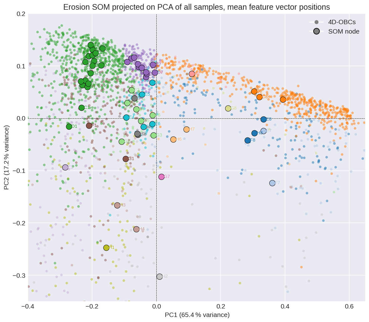
Figure A2 Space defined by the first two principal components of the features of the erosion 4D-OBCs. Small dots indicate transformed 4D-OBC positions in PCA space, larger dots indicate the transformed location of the mean feature vectors of the Self-organizing Map (SOM). The colours relate to the colours in Fig. 8.

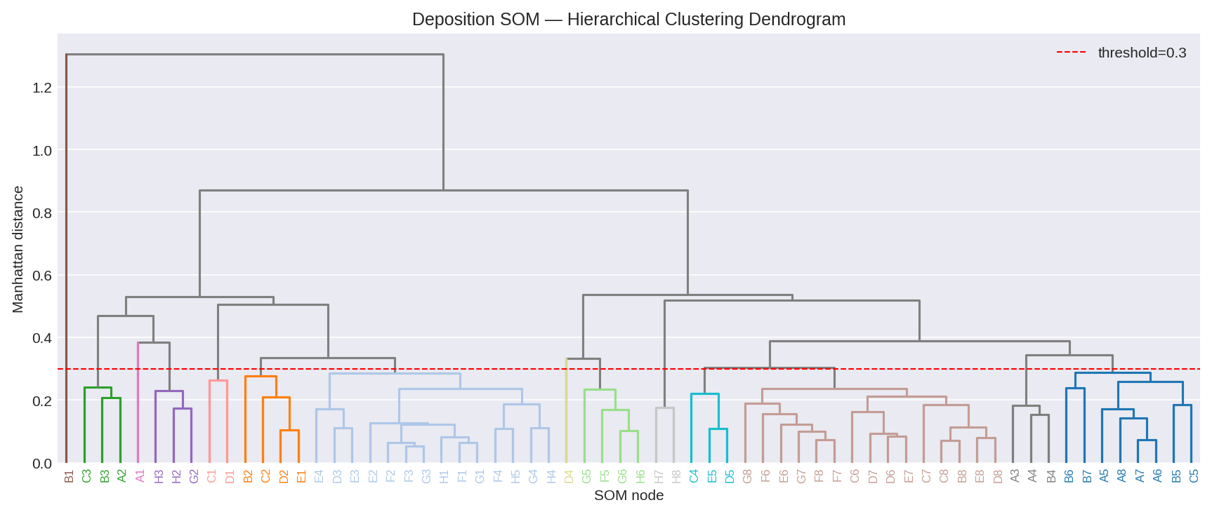
Figure A3 Dendrogram following the hierarchical clustering of the Deposition Self-organizing Map (D-SOM). The red dashed line indicates the chosen cut-off point. The colours relate to the colours in Fig. 8. The y-axis shows the Manhattan distance at which clusters are merged. X-axis labels indicate the respective SOM node.

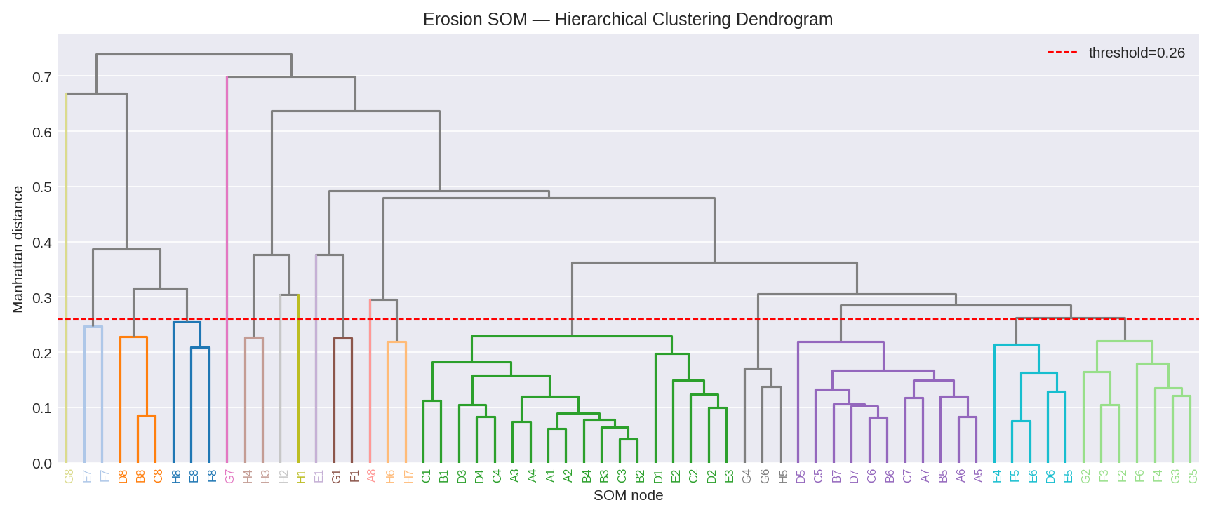
Figure A4 Dendrogram following the hierarchical clustering of the Deposition Self-organizing Map (D-SOM). The red dashed line indicates the chosen cut-off point. The colours relate to the colours in Fig. 8. The y-axis shows the Manhattan distance at which clusters are merged. X-axis labels indicate the respective SOM node.