Evolution of seepage driven networks in the lab

During rain, water infiltrates the ground, where it flows as groundwater toward nearby rivers. There, its emergence can entrain sediments, triggering seepage erosion and thereby influencing the development and expansion of river networks. To investigate this process, we construct an experimental aquifer, made of erodible plastic sediments. A reservoir beneath the aquifer supplies water at a controlled recharge rate. We find that seepage erosion, driven by the resulting groundwater flow, is sufficient to initiate the formation and growth of a drainage network. For a given recharge rate, network growth eventually ceases as the drainage system reaches a steady-state morphology, in which sediments are everywhere at the threshold of motion. This observation indicates that the recharge rate of the aquifer selects the size of the network. In our experiment, the depth of the aquifer is small compared to its lateral extent, so that the flow of groundwater obeys the Dupuit-Boussinesq equation. As in natural systems, the water table in our experiment intersects the drainage network at the elevation of the streams. This condition provides the necessary boundary conditions to solve for the Dupuit-Boussinesq equation and reconstruct the shape of the water table around the river network. The resulting numerical solution agrees well with piezometric measurements carried out in the experimental aquifer and reveals that groundwater flow converges toward channel tips, where its flux is maximal.

1 Introduction

During rain, water infiltrates the unsaturated porous ground and travels downward until it reaches the saturated region of an aquifer. There, it flows as groundwater (Guérin et al., 2019). When the free surface of this groundwater flow, known as the water table, intersects with the land surface, water seeps out of the aquifer and flows onto the ground surface. If groundwater emerges with enough strength, it entrains sediment particles and digs a channel (Dunne, 1980, 1990; Vulliet, 2023; Howard and McLane, 1988). At the tip of this channel, erosion gradually undermines the land, which collapses and forms a receding erosion front (Higgins, 1982; Devauchelle et al., 2011). The recession of this front modifies the flow in the surrounding aquifer, which converges towards the channel tip, thereby amplifying its erosion (Petroff et al., 2011). This process, known as seepage erosion, controls the growth and shape of river heads. It may also cause river heads to split into two new channels, leading to the formation of a branching drainage network (Dunne, 1980; Dietrich and Dunne, 1993; Devauchelle et al., 2012; Petroff et al., 2012, 2013).

To understand the growth of a drainage network we must, on one hand, reconstruct the groundwater flow in the catchment, and, on the other hand, understand how this flow controls seepage erosion. In a catchment, when the horizontal extent of the aquifer is much larger than its depth, the Dupuit-Boussinesq approximation states that vertical movements of the groundwater flow can be neglected at leading order (Dupuit, 1863; Boussinesq, 1877). The elevation of the water table relative to the aquifer bottom, h, thus follows the Dupuit-Boussinesq equation, which, averaged over a long-time period, takes the form of a Poisson equation,

$$\begin{array}{}\text{(1)}& {\mathrm{\nabla }}^{\mathrm{2}}{h}^{\mathrm{2}}=-{\displaystyle \frac{\mathrm{2}R}{K}},\end{array}$$

where R is the recharge rate of the aquifer and K is a hydraulic conductivity representative of the catchment.

Field observations have long demonstrated that groundwater flow converges toward drainage networks, where the water table intersects the drainage system at an elevation equal to the river level. Making use of this observation, Petroff et al. (2011) and Devauchelle et al. (2012) used the elevation of the river network – taken as a proxy for river water levels – as a boundary condition to solve Eq. (1) and reconstruct groundwater flow in a small catchment in the Florida Panhandle. They found that groundwater flow mainly converges towards channel heads, where the discharge of groundwater into the drainage network is maximum (Abrams et al., 2009; Petroff et al., 2012, 2013; Devauchelle et al., 2012). This amplification of discharge concentrates seepage erosion at channel heads, and controls the growth of the drainage network.

Field data suggest that the formation of a drainage network is a slow process, with characteristic growth rates around a few mm per year, a timescale way too long to allow for direct monitoring in the field (Abrams et al., 2009). To bypass this issue, several authors chose to investigate channel growth in laboratory experiments by forcing groundwater through an erodible aquifer made of granular material. When the groundwater discharge exceeds a threshold, the water flowing out of the aquifer entrains grains, and erodes its surface over timescales that range from a few hours to a few days (Lobkovsky et al., 2004; Schorghofer et al., 2004). The morphology resulting from this seepage erosion depends on the geometry of the experimental setup.

If the experiment takes place in a narrow flume, seepage erosion forms a quasi-2D erosion front, which retreats at a velocity that decreases over time (Howard and McLane, 1988; Howard, 1988; Kochel et al., 1988). Eventually, erosion ceases and the front relaxes into a steady, equilibrium shape (Vulliet, 2023). When the flume is wide enough, seepage erosion incises a channel, whose evolution depends on the way water is delivered to the aquifer. When water is injected from an adjacent reservoir maintained at constant water level, the channel usually dies without bifurcating. Conversely, when the aquifer is recharged with a homogeneous rainfall, the probability to observe a bifurcation increases (Gomez and Mullen, 1992; Berhanu et al., 2012; Sockness and Gran, 2022). In addition, the use of angular grains and larger setups appears to promote the development of branching networks (Pornprommin et al., 2010; Pornprommin and Izumi, 2010).

In this article, we use a laboratory aquifer to investigate the growth of drainage networks driven by seepage erosion. We find that this process is capable of forming a drainage network of at least a few channels. As the network expands, the flow of groundwater around it evolves to accommodate this change of boundary conditions. This feedback, in turn, governs channel growth. The article begins with a description of our experimental setup and procedures. We then present in detail a representative experimental run, and focus on the influence of the aquifer recharge on the growth of the network. In the third part, we use the Dupuit-Boussinesq equation to reconstruct the elevation of the water table around the drainage network, and compare the results with piezometric measurements. The reconstructed water table allows us to estimate the direction and magnitude of the groundwater flow around the network, and to discuss its influence on the growth of the drainage network.

2 Seepage erosion in a laboratory aquifer

We conducted our experiments in a rectangular tank of height 35 cm and dimensions 150×150 cm² (Fig. 1). A thin (1 cm thick) layer of felt, held between two metal grids and positioned 15 cm above the bottom of the tank, divides the latter into two compartments. On top of the felt, we pour a layer of plastic sand (Guyson guyblast plastic media US type 2). This layer of plastic grains forms our experimental aquifer, and the felt layer serves as its bottom. Depending on the experiment, the thickness of the aquifer varies between 15 and 20 cm. The plastic sand is made of relatively uniform grains, with sizes ranging from d=500 to 1000 µm and density ρ=1500 kg m⁻³. Its friction coefficient is μ≃0.9 and its porosity, ω, is around 45 % (Abramian et al., 2020; Popović et al., 2021).

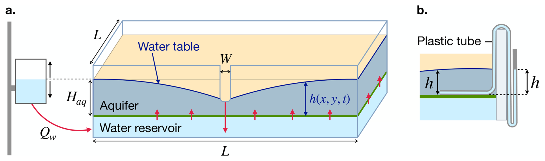
Figure 1 (a) Experimental setup. The green line represents the felt layer that separates the aquifer from the water reservoir used to recharge the aquifer. (b) Schematics of the plastic tubes used as piezometers to measure the water table height, h.

The method most commonly used to induce groundwater flow through the aquifer is to apply an artificial rain above the setup by mean of a sprinkler (Berhanu et al., 2012). However, this approach poses several problems: (i) rain prevents clear imaging of the aquifer surface, (ii) raindrop impacts can erode surface grains through splash effects, and (iii) excessively high rainfall rates can generate runoff, which in turn induces surface erosion. To avoid these inconveniences, we supply water to the aquifer from below. To do so, we use the lower part of the tank as a reservoir, into which we inject water at a constant discharge rate, Q_w, set by an overflowing tank (Fig. 1). As water fills this reservoir, its level rises until it reaches the metal grid and seeps through the felt layer into the overlying plastic sand. The hydraulic conductivity of the felt, about $\mathrm{4.6}\times {\mathrm{10}}^{-\mathrm{5}}$ m s⁻¹, is two orders of magnitude smaller than that of the overlying sand. Consequently, the felt layer builds pressure in the reservoir and distributes the water recharge uniformly across the base of the sand aquifer.

The overflowing tank feeding the aquifer is mounted on a platform, whose elevation can be adjusted by mean of a motor controlled by a computer (Fig. 1). Setting the elevation of the overflowing tank allows us to control the recharge rate of the aquifer, $R=Q_{\mathrm{w}}/A$, where A=2.25 m² is the surface of the aquifer.

A 5 cm wide rectangular opening, cut in the center of one of the tank walls, 15 cm above the aquifer bottom, serves as an outlet, which allows both water and sediment grains to exit the tank (Fig. 1). As water fills the aquifer, its free surface eventually reaches the level of the outlet. Groundwater then converges toward the opening, flows through the outlet and leaves the tank. The wide range of recharges used in our experiments, from 0.1 to 10 L min⁻¹, precludes the use of an electronic flowmeter. Instead, we measure water discharge by regularly collecting in a beaker the mixture of water and sediments flowing out of the tank over time intervals ranging from 1 to 5 min. Because the sediment discharge is relatively low (about 20 g h⁻¹) compared with the water discharge (at least 6 kg h⁻¹), the sediment mass is negligible. Weighing the beaker thus yields a reliable estimate of the water discharge (Romon, 2025).

A camera positioned approximately 1.5 m above the aquifer surface, captures images of our setup every minute. LED panels, placed on the sides of the experiment, provide uniform lighting. The images show that groundwater flow at the outlet is strong enough to entrain plastic grains and erode the aquifer. Seepage erosion thus gradually forms one or several channels that originate at the outlet (Fig. 2a). These channels grow backward, with heads that take on an amphitheater shape, as seepage driven channels usually do (Lamb et al., 2006). As the surface of the aquifer lies a few cm above the outlet, channels are 1 to 5 cm deep with relatively steep riverbanks.

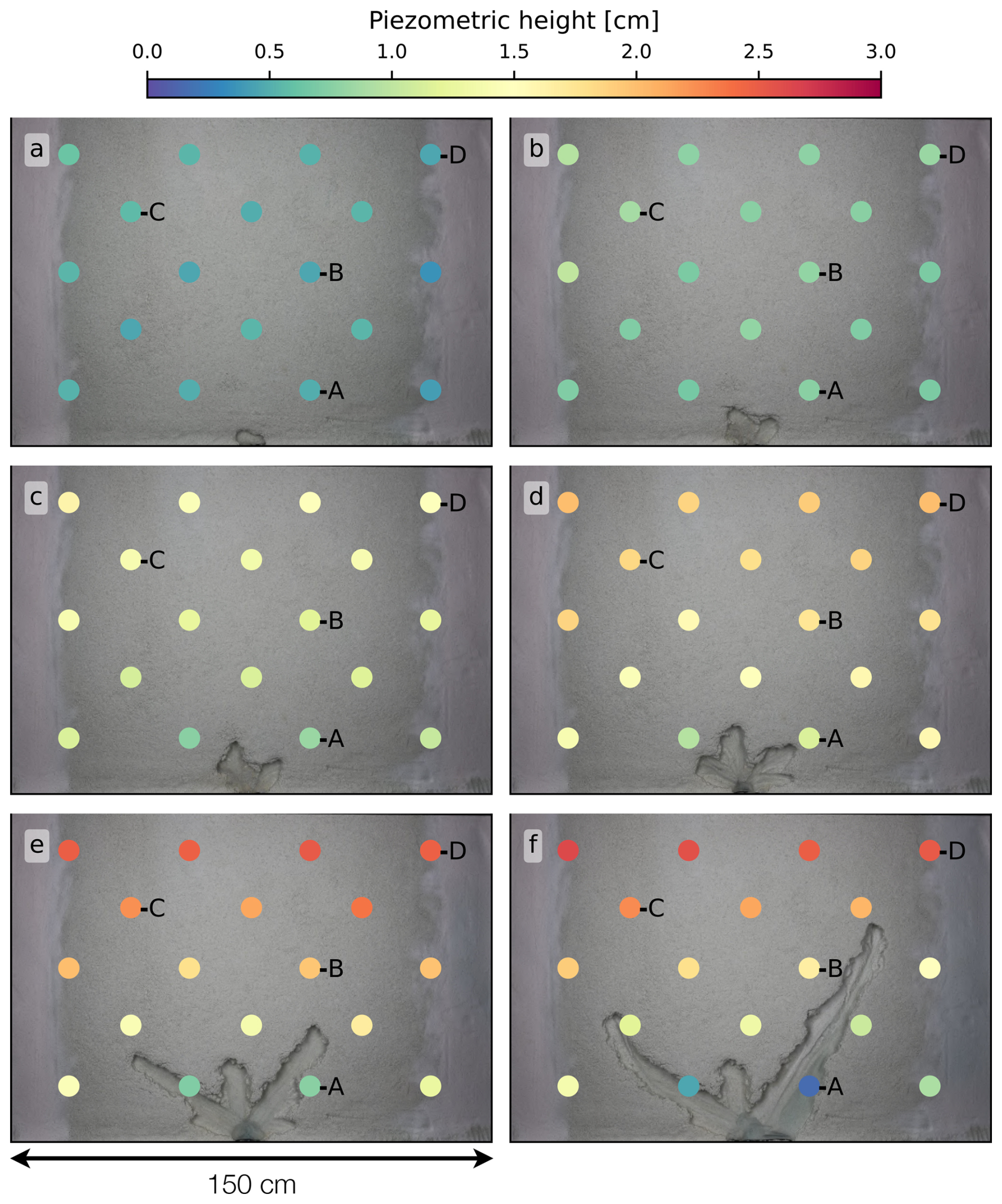
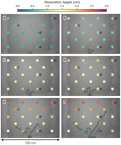
Figure 2 Images of steady-state drainage networks obtained at increasing recharge rates. Panels (a)–(f) correspond to discharge rates Q=0.1, 0.7, 1.2, 1.6, 2.0, and 2.6 L min⁻¹, respectively. Colored markers indicate the locations of the piezometers, with a color scheme that represents the local water-table height relative to the elevation of the outlet. In panel (d), two channels on the right side of the network are distinct, whereas in panel (f) they have merged into a single channel (see Video supplement).

To characterize the flow in the aquifer, we measure the groundwater pressure by mean of 22 piezometers uniformly distributed along the aquifer bottom. Each piezometer consists of a plastic tube (3 or 6 mm in inner diameter), with its tip positioned at various locations across the bottom of the aquifer (Figs. 1b and 3). The tube diameter narrows at its tip, allowing water to enter while preventing grain intrusion. The tube runs along the aquifer bottom, passes over and down the opposite side of the experimental wall, and rises to form a vertical column (Fig. 1b). During an experiment, groundwater fills the tube until its level in the vertical column equilibrates with the pressure at the aquifer bottom. Using a second camera, we acquire images of these vertical columns, from which we measure the water level in the piezometers every 5 min.

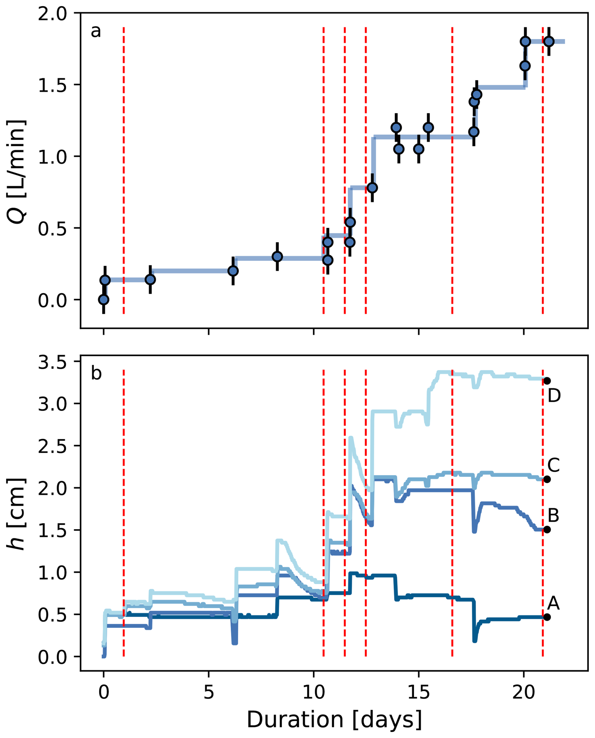
Figure 3 (a) Discharge at the outlet of the aquifer vs. time (in days) during the experiment presented in Sect. 3. Blue bullets: experimental measurements. Solid line: fit of a step function to the data. (b) Water table height in four piezometers vs. time (in days) during the same experiment. The position of the piezometers is shown on Fig. 2. Red dashed lines: moment of each image from Fig. 2.

The depth of our aquifer (H≃15 cm) is much smaller than its lateral extent (L=150 cm). In this configuration, groundwater flow satisfies the Dupuit–Boussinesq approximation, and the groundwater pressure is hydrostatic at a leading order (Dupuit, 1863; Boussinesq, 1877). As a result, the water level in our piezometers provides a direct measurement of the water table height relative to the aquifer bottom, h.

To investigate the formation of drainage networks in our laboratory aquifer, we ran several preliminary experimental runs, each lasting from a few days to a couple of weeks (see Appendix A). Each run began with the lowest recharge achievable with our setup (Q_w≃0.1 L min⁻¹). In every case, seepage erosion immediately carved a channel originating from the outlet (Fig. 2a). Over time, however, erosion gradually slowed and eventually stopped, with no further activity observed even after 12 h. The only way to reactivate erosion was to increase the aquifer recharge, which immediately triggered new channel growth until it ceased again. These observations suggest that, for a given recharge rate, network growth eventually ceases as the drainage system relaxes to a steady-state morphology, in which sediments are everywhere at the threshold of motion. If this interpretation is correct, the aquifer recharge should effectively select the size of this steady-state network. In the next section, we discuss in detail an experimental run specifically designed to test this hypothesis.

3 Influence of the aquifer recharge on the growth of the drainage network

To investigate how the recharge of the aquifer controls the size of the network, we followed a stepwise experimental procedure. We began this experiment at the lowest achievable recharge rate with our setup (Q_w≃0.1 L min⁻¹), and let it run for several hours after erosion had ceased. To ensure that no further channel growth occurred, we compared photographs from different time periods and waited until an absence of observable changes indicated that the network had reached a stable morphology. At that point, we measured the discharge of water leaving the aquifer, increased the recharge by a small amount (typically 0.1 L min⁻¹), then measured discharge once more (Fig. 3a). Over the course of 25 d – during which the experiment ran continuously – we repeated the procedure, thus increasing the recharge a total of 10 times, and observed how the shape of the resulting stable network evolved with the aquifer recharge (Fig. 3a).

In the course of this experiment, we found that seepage erosion caused the growth of several channels (see Video supplement). The shape of the resulting network, depended on the competition between two opposite processes. On one hand, channel heads regularly split, dividing into two channels (Fig. 2d). On the other hand, channels gradually widened, sometimes merging with neighbors to form a single wider channel (Fig. 2f).

Piezometric data allowed us to monitor how the growth of the drainage network affected the surrounding groundwater flow. We found that each increase in aquifer recharge caused a quasi-immediate rise of the water level in each piezometer, which then gradually relaxed toward a stable value as the drainage network approached its equilibrium morphology (Fig. 3b). In this steady state, the water table height decreases towards the drainage network, where its value reaches a minimum (Fig. 2).

To understand how the size of the drainage network relates to total aquifer recharge, we systematically measured the area of the network, once it had reached steady state. To do so, we manually traced the contours of the network on the experimental images, and calculated the area enclosed by each contour (Fig. 2). Repeating this process several times allowed us to estimate the measurement accuracy to be within less than 4 %. The resulting data suggest that the area of a stable drainage network increases linearly with recharge (Fig. 4). As we only conducted a single experiment, it is impossible to draw definitive conclusions. But we speculate that the relationship might also depend on the properties of the aquifer, such as hydraulic conductivity and grain size.

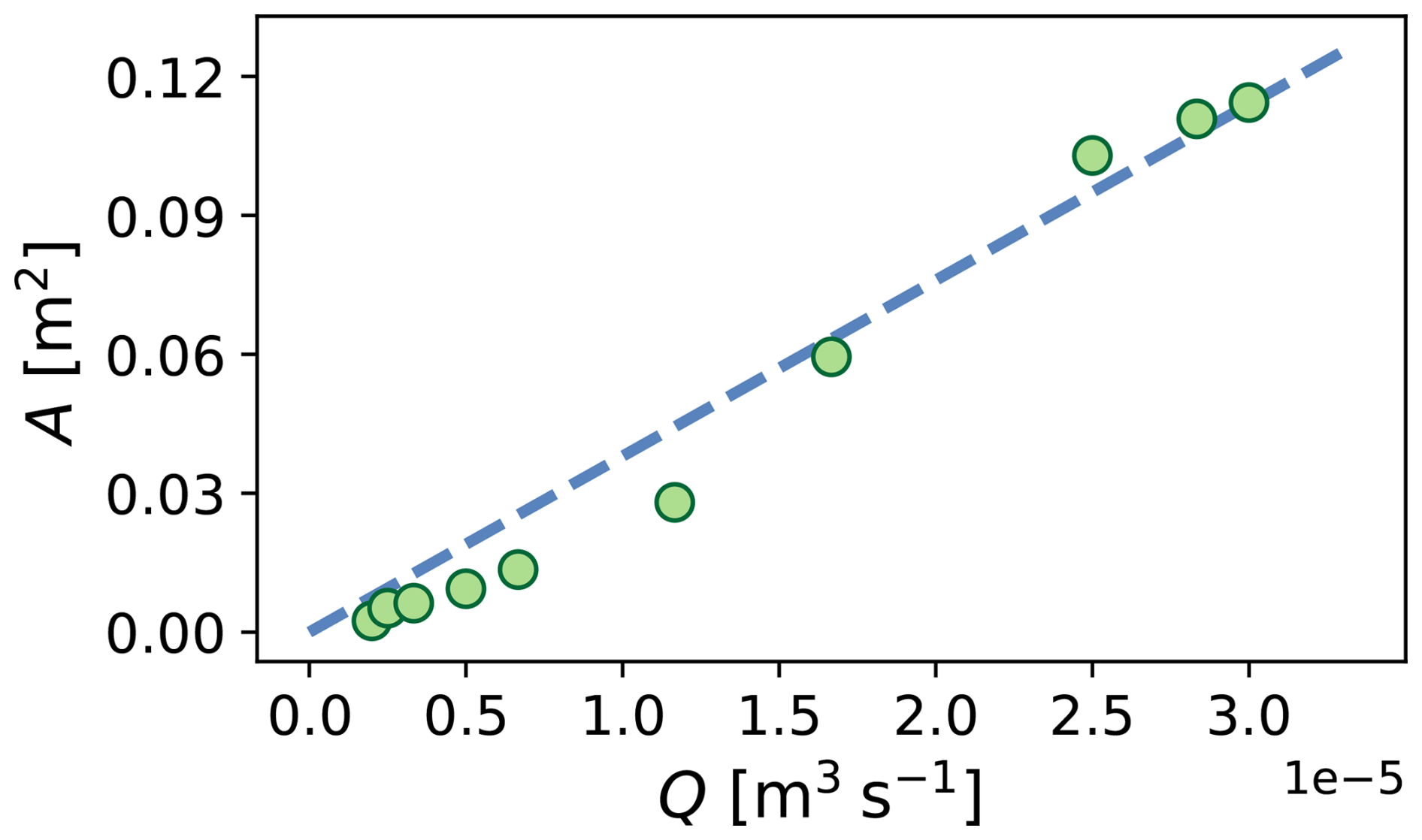
Figure 4 Network area, A, as a function of the aquifer recharge, Q, during the experiment presented in Sect. 3. Blue dashed line: linear fit to the data A=αQ with $\mathit{\alpha }=\mathrm{3.8}\times {\mathrm{10}}^{\mathrm{3}}$ s m⁻¹.

In this experiment, as in all others, we never observed overland flow outside the channels forming the drainage network. The growth of the network is therefore entirely controlled by seepage erosion, induced by the flow of groundwater in the aquifer. In the next section, we therefore focus on groundwater with the objective to reconstruct the water table around the network.

4 Groundwater flow

Each increase in recharge triggers a transient phase, during which the drainage network grows through seepage erosion, while the groundwater flow adapts to the resulting change of boundary condition. Eventually, however, the network and the groundwater flow reach a new steady-state. Assuming the Dupuit-Boussinesq approximation holds in this regime, the water table elevation, h, follows a Poisson equation,

$$\begin{array}{}\text{(2)}& {\mathbf{\nabla }}^{\mathrm{2}}{h}^{\mathrm{2}}=-{\displaystyle \frac{\mathrm{2}R}{K}},\end{array}$$

where K is the hydraulic conductivity of our aquifer, and R is the recharge rate.

To solve Eq. (2), we must complement it with boundary conditions. The walls bounding the aquifer are impervious. Therefore, the normal velocity of groundwater vanishes along them, a condition that reads ${\partial }_{n}h=\mathrm{0}$, where n denotes the direction normal to the wall.

The drainage network provides a second boundary condition: the water table intersects the network at the elevation of the streams (Petroff et al., 2012; Devauchelle et al., 2011, 2012). Applying this boundary condition requires to evaluate the elevation of the free surface of the channels that form the drainage network. In practice, this is a challenging task as these streams are only a few millimeters deep. Following Petroff et al. (2011), we therefore neglect the depth of the streams, and approximate the elevation of their free-surface by that of their bed. Because the longitudinal slope of the channels is small (less than 3 %), we further simplify the problem by neglecting the network topography. Consequently, we set the elevation of the entire drainage network equal to that of the outlet. With these approximations, the boundary condition reduces to h=0 along the contour of the drainage network.

To compute the shape of the water table, we solve Eq. (2) subject to the two boundary conditions derived above.

Before doing so, however, we must evaluate the source term $R/K$. Measurements of the discharge at the outlet of the experimental tank provide the recharge rate R. The hydraulic conductivity of the plastic sand was measured using a Darcy column, giving a value of $K=\mathrm{2.9}\times {\mathrm{10}}^{-\mathrm{3}}$ m s⁻¹. As the packing of the sand bed in our experiment is much more loose than in a Darcy columns – where grains are compacted to avoid the accumulation of air bubbles, we expect the true hydraulic conductivity of our aquifer to be higher.

To test this hypothesis, we proceed by iterations. We first assign an arbitrary value to the hydraulic conductivity. Using pyFreeFEM (Devauchelle, 2025), a Python wrapper for the finite-element software FreeFEM++ (Hecht, 2024), we build a numerical mesh that covers the entire surface of the experimental setup. To improve the accuracy of the calculation, we refine the mesh in regions where the gradient of the water-table elevation is large (Fig. 5a). We then apply the finite-element method to solve Eq. (2) on this mesh (Romon, 2025). The resulting solution provides us with a numerical reconstruction of the water table around the experimental drainage network at steady-state (Fig. 5a).

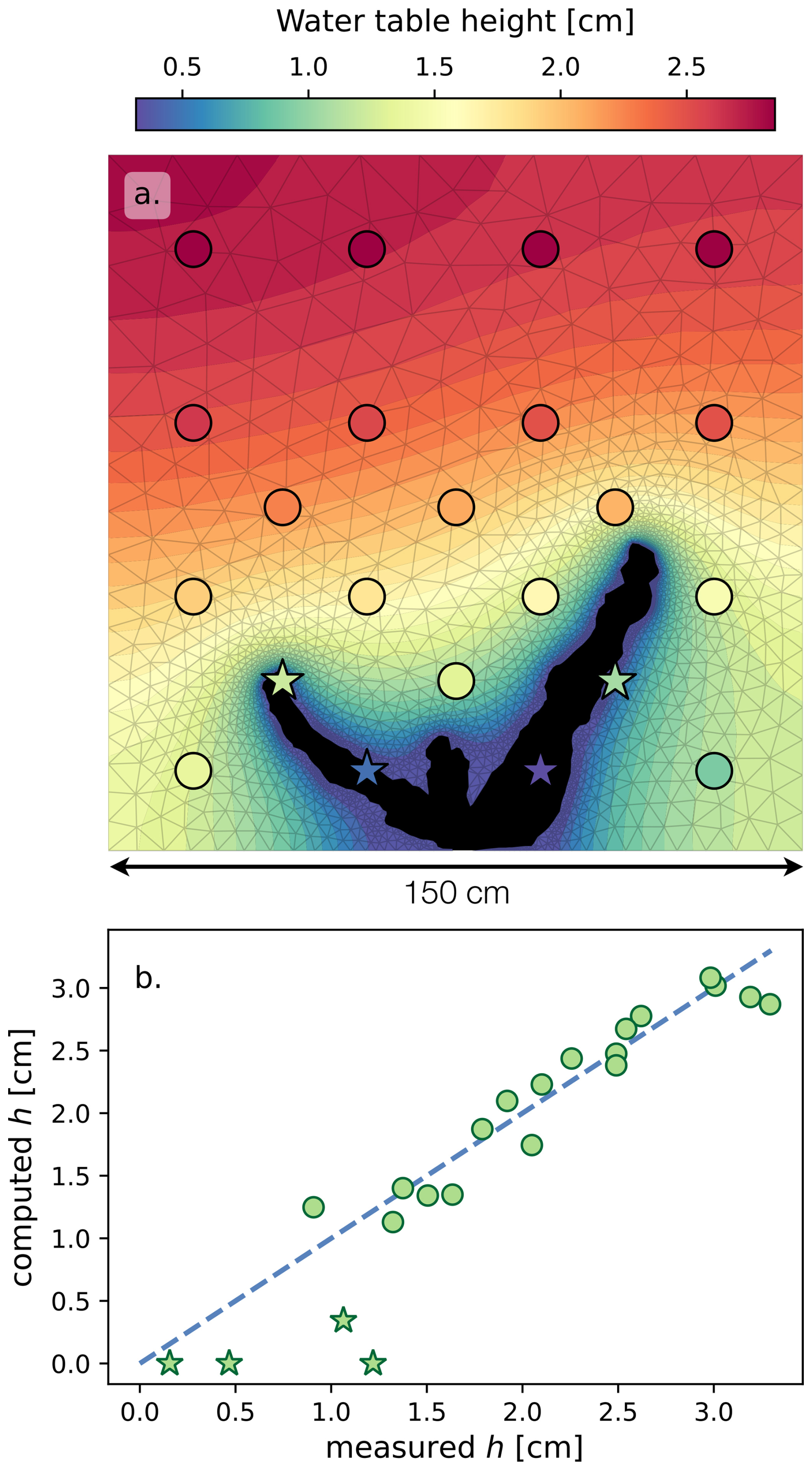
Figure 5 (a) Reconstruction of the water-table height, h, around the steady-state network of Fig. 2f. The black area corresponds to the drainage network. Colors indicate the water-table height computed from Eq. (2) for $K=\mathrm{4.1}\times {\mathrm{10}}^{\mathrm{-}\mathrm{3}}$ m s⁻¹. Colored markers show the position and water level of each piezometer. Light gray triangles indicate the numerical mesh used to compute the water table. (b) Computed water-table height versus experimental measurements. The dashed line is the identity line (x=y). In both panels, bullets mark piezometers located outside the drainage network, while stars indicate piezometers inside the drainage network.

To assess the quality of this reconstruction, we compare it to the piezometric measurements in our 22 piezometers. We then use an iterative optimization procedure to adjust the hydraulic conductivity to the value that minimizes the difference between the numerical reconstruction and the experimental data. This procedure yields $K\simeq \mathrm{4.1}\times {\mathrm{10}}^{-\mathrm{3}}$ m s⁻¹. As expected, this value is higher yet close to that obtained by measurements in Darcy columns.

The optimized solution accurately reproduces the water-table height in all piezometers, except for those located inside or near the network (Fig. 5b). This discrepancy is expected, as the boundary condition within the network, h=0, is only an approximation of the true network topography and does not account for the finite water depth in the channels. The difference between our boundary condition and the actual water table height inside the drainage network (approximately 1 cm) results in an overestimation of the groundwater flux by a factor of about two (see Appendix B).

In short, our numerical method accurately reproduces the water table, except in the immediate vicinity of the drainage network. We therefore apply it to reconstruct the water table around the drainage network presented in Sect. 3, at various stages of its growth. The results suggest that the extent over which the network influences the shape of the water table is roughly proportional to the size of the network. Indeed, close to the network, the iso-heads – lines of constant water table elevation h – bend to follow the shape of the network (Fig. 6a–c). At larger distances, however, the iso-heads gradually smooth out, as the network’s influence decreases.

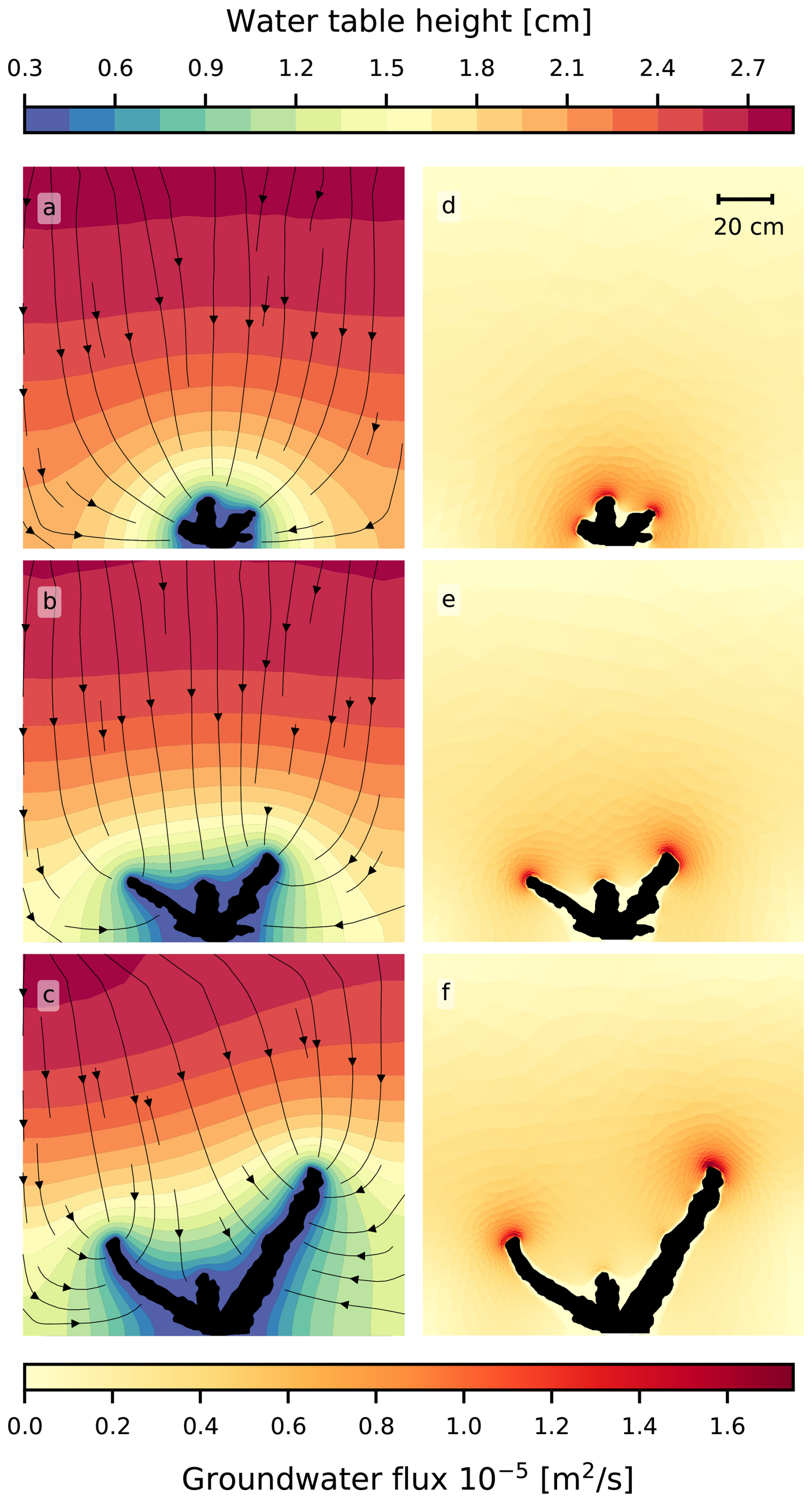
Figure 6 (a–c) Reconstruction of the water-table height around the steady-state networks of Fig. 2d–f. Black lines with arrows indicate flow streamlines, showing the main flow directions and convergence toward the drainage channels. (d–f) Corresponding magnitude of the groundwater flux. Each reconstruction of the water table and of the associated groundwater flux spans over the entire experimental aquifer (150×150 cm).

From the reconstructed water table elevation, we compute the gradient, ∇h, and draw the corresponding streamlines (Fig. 6a–c). We find that these streamlines converge towards the drainage network, and concentrate near channel tips. Accordingly, the groundwater flux, $q=-Kh\mathrm{\nabla }h$, increases close to the channel tips, reaching values much higher than in the rest of the aquifer (Fig. 6d–f). In short, groundwater flow converges toward channel tips, where its flux is maximal. These observations, consistent with those of Devauchelle et al. (2012), explain why network growth occurs preferentially at the tips: a larger groundwater flux enhances seepage erosion at channel heads, while the flux along the sides of the channels is too low to trigger erosion (Devauchelle et al., 2012; Petroff et al., 2012, 2013).

5 Conclusions and Discussions

The experiments presented in this paper demonstrate that seepage erosion alone can initiate the formation and growth of a drainage network. They further show that, for a given recharge rate, network growth eventually ceases as the system reaches a steady-state morphology, in which sediments are everywhere close to the threshold of motion (Vulliet, 2023). The size of the resulting steady-state network appears to increase roughly linearly with aquifer recharge. Establishing the exact nature of this relationship requires additional experiments. Moreover, precise measurements of the sediment flux would improve our ability to monitor the erosion intensity during network growth, which we currently assess only through visual observations.

If these findings apply in natural settings, they suggest that in areas where infiltration dominates over overland flow, many natural networks may operate near steady state. Under these conditions, network size likely reflects the intensity of local recharge. This interpretation, however, requires caution. Natural drainage networks evolve over long timescales, and some areas likely experienced stronger aquifer recharge in the past. As a result, the morphology we observe today may not reflect current recharge conditions but instead preserve remnants of past hydrological regimes. We observed such a case during a field campaign in the Sanwara catchment, a small basin in central India. At the time of our visit in the summer of 2024, water did not flow in the upper part of the network despite a heavy monsoon (Romon, 2025). The drainage network was therefore likely carved during a period when aquifer recharge and groundwater flow were more intense.

Our experimental results also show that it is possible to reconstruct the water table in the aquifer using the shape of the drainage network. Based on this method, we find that groundwater converges toward channel tips, where the groundwater flux is maximal. This explains why network growth occurs preferentially at the tips (Devauchelle et al., 2012; Petroff et al., 2012, 2013). However, to reconstruct the water table, we choose to neglect the network topography and set it to zero. While this method correctly captures the shape of the water table across most of the experimental domain, it overpredicts the discharge by a factor of about two near the channel tips. Measuring the topography would help us to resolve this discrepancy. Unfortunately, because of their homogeneous color, our grains lack the texture required to use photogrammetry. We are instead currently testing a fringe projection method to extract the topography (Takeda and Mutoh, 1983; Maurel et al., 2009).

Unlike our experimental setup – where the network is isolated within a finite domain – the growth of natural networks is also constrained by their interaction with neighboring networks, which might limit the extent of their drainage areas. To test and extend our findings, we need to conduct further experimental and field work. In particular, we aim to compute accurate estimates of the groundwater velocity in the aquifer, in order to predict of erosion rates, and compare them with estimates from natural networks (Abrams et al., 2009; Cohen et al., 2015).

Beyond its application to seepage erosion, the method for reconstructing the water table has many other potential uses. In particular, we are currently working to extend this method to field settings, with the goal to estimate groundwater flow, storage, and river discharge from topographic maps, in areas where piezometric data are unavailable (Romon, 2025).

Appendix A: Observations from preliminary experiments

To investigate the growth of drainage networks in our laboratory aquifer, we ran five preliminary experiments. Several of these experiments led to the formation of branching river networks (Fig. A1). In each case, the growth of the network followed the same pattern as that described in Sects. 2 and 3. At the start of an experimental run, one or two channels formed near the outlet and grew outward until they split and formed new branches, which competed with one another for drainage area and groundwater flow (Dunne, 1980; Devauchelle et al., 2012). Each increase in aquifer recharge led to a peak in erosion, which rapidly decreased to negligible levels. While most of the erosion occurred near the channel tip, erosion of the river banks led to channels widening, and often to the merging of neighboring channels (Fig. A1).

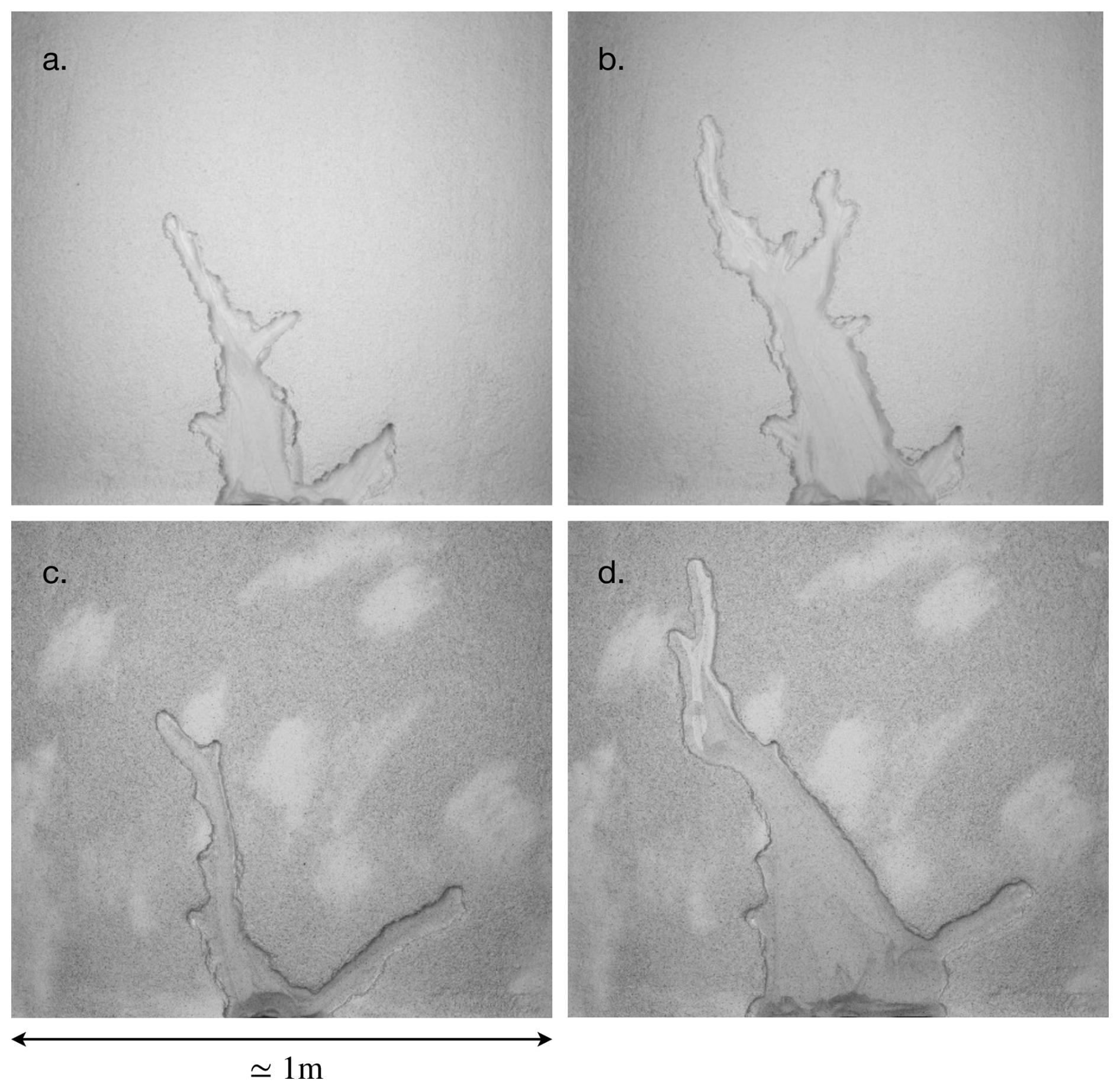
Figure A1 Pictures of 2 preliminary experiments (a–b, c–d) at different states of the branching networks evolution.

Appendix B: Evaluation of the error on the groundwater flux computations

In Sect. 4, we solved for the groundwater flow in the aquifer under the simplifying assumption that the network topography is negligible. In this section, we evaluate the error that this assumption induces. To do so, we discuss the case of a simpler, one-dimensional system meant to represent a small section of our experiment in the vicinity of a channel tip (Fig. B1). Because we consider only a small portion of the experiment, we assume that the influence of the aquifer recharge can be neglected. In this one-dimensional configuration, the water table height, h, admits the following analytical solution (Bear, 1972; Métivier, 2026),

$$\begin{array}{}\text{(B1)}& h^{\mathrm{2}}=\left({\displaystyle \frac{h_{\mathrm{r}}^{\mathrm{2}}-h_{\mathrm{up}}^{\mathrm{2}}}{L}}\right)x+h_{\mathrm{r}},\end{array}$$

where h_r and h_up are the water table heights at two points near the river tip: the first inside the drainage network and the second one outside it. L is the distance between these two points (Fig. B1). Combining Eq. (B1) with the expression of the groundwater flux, $q=-Kh{\partial }_{x}h$, we find:

$$\begin{array}{}\text{(B2)}& q=-{\displaystyle \frac{K}{\mathrm{2}}}\left({\displaystyle \frac{h_{\mathrm{r}}^{\mathrm{2}}-h_{\mathrm{up}}^{\mathrm{2}}}{L}}\right).\end{array}$$

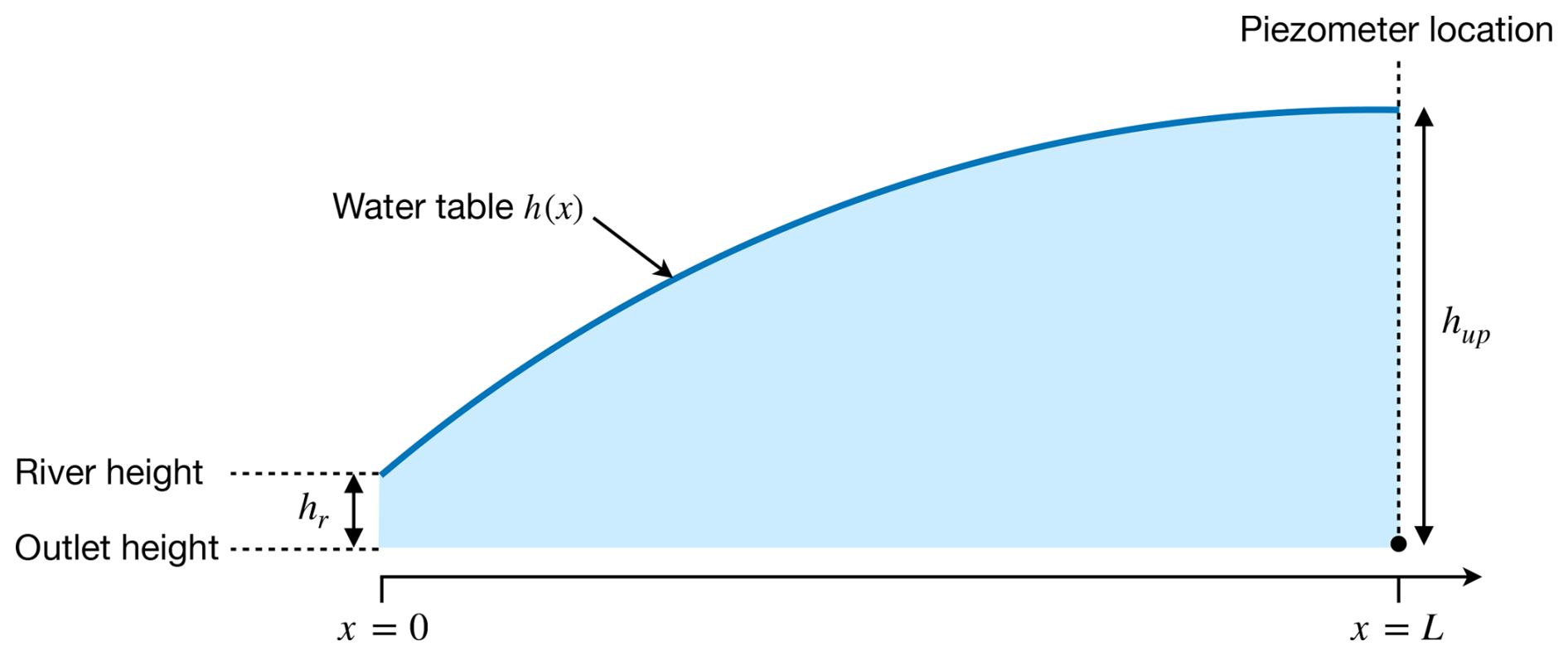
Figure B1 Vertical section of the water table in our experiment, between the tip of a river (x=0) and the closest piezometer (x=L).

According to the piezometric data (Fig. 5), we estimate h_up≃1.8 cm, h_r≃1.3 cm and L=25 cm. Conversely, our numerical simplification sets h_r=0. Using Eq. (B2), we compare estimates of the groundwater flux for both values of h_r, and find that the flux computed with our simplification, $q(h_{\mathrm{r}}=\mathrm{0}\mathrm{cm})\simeq \mathrm{2.7}\times {\mathrm{10}}^{-\mathrm{6}}$ m s⁻¹, is twice as high as the one computed with the piezometric data, $q(h_{\mathrm{r}}=\mathrm{1.3}\mathrm{cm})\simeq \mathrm{1.3}\times {\mathrm{10}}^{-\mathrm{6}}$ m s⁻¹.