Lift or impact: modelling bedrock incision coupled with sediment dynamics

We analyze how the process of bedrock incision by the impact of sediment grains can be described and coupled with sediment dynamics. We first point out that the key parameter is a bedrock dimensionless coefficient that describes the ratio between the volumes of impacting sediments and bedrock erosion. We then write the coupled equations by introducing a partitioning coefficient between sediment and bedrock erosion. It describes the time spent undergoing one or the other erosion process – or the proportion of depositing grains that impact bedrock. In a 1D along-stream system, the resulting equations lead to a similar description of the cover effect proposed by Sklar and Dietrich (2004), giving a rationale to their expression. In a second step, we extend the concept to lateral erosion or deposition fluxes. We develop analytical solutions for a river fed by uniform lateral sediment fluxes from hillslopes and show why the sediment load can exceed the transport capacity. We then implement the equations in the numerical code River.lab/eros, where water depth and velocity, as well as erosion and deposition fluxes, are solved with the method of precipitons. As an example, we simulate the evolution of the Rheinfall at Schaffhausen, Switzerland, a prominent knickpoint along the Hochrhein. In contrast with sediment processes, where the knickpoint slope decreases by diffusion without upstream displacements, bedrock abrasion allows knickpoints to move upstream while retaining almost the same shape. This is consistent with detachment-limited behaviour as emphasized in the theoretical part of the paper. The knickpoint shape (foot elevation and height) and retreat rates are highly dependent on the sediment load in the river. Bedrock erosion first occurs in a narrow canyon that propagates upstream, and then the river widens after the knickpoint has passed by.

1 Introduction

The erosion of bedrock by the impact of sedimentary grains is a key process in the erosion of mountain ranges, yet it is rarely included in studies of landscape evolution. The predominant role of sediment grain impact on bedrock erosion was proposed qualitatively (e.g., Gilbert, 1877; Foley, 1980) and then confirmed by laboratory erosion experiments (e.g., Auel et al., 2017; Scheingross et al., 2014; Sklar and Dietrich, 2001). It implies that bedrock erosion rates depend primarily on sediment fluxes. This contrasts with transport-limited or detachment-limited theories, in which the erosion rates are proportional to the deviation from the theoretical transport capacity or the stream power of the river, respectively. A simplified formulation of the erosion rate has been proposed by Sklar and Dietrich (2004) (referred to as SD2004) and further corrected and/or developed (Sklar and Dietrich, 2012; Lamb et al., 2015; Chatanantavet et al., 2013; Turowski et al., 2007; Auel et al., 2017; Turowski et al., 2023; Demiral et al., 2026). It considers the erosion rate as the product of the number of impacts per unit of time and the amount of material removed with each impact, considering the impact energy. Although the latter term is debated, specifically, which rock property controls impact erosion and the mass extracted by impacts (Beer and Lamb, 2021; Scheingross et al., 2014; Turowski et al., 2023; Litwin Miller and Jerolmack, 2021), the decomposition into two components – the first depending on sediment bedload flux and the latter on rock mechanics – remains a fundamental aspect of bedrock incision theory.

An additional complexity is that bedrock erosion can be prevented by an immobile (or slightly mobile) sediment cover, which led SD2004 to introduce a third term in the incision rate related to the deviation from transport capacity. The rationale is that the thickness of the sediment cover, if it exists, is mainly controlled by this term, although other complexities, such as the role of bed roughness, also play a role in the cover dynamics (Chatanantavet and Parker, 2008; Hodge and Hoey, 2012; Johnson, 2014). The cover effect illustrates how erosion driven by the impact of sediment grains is closely intertwined with sediment dynamics, since it produces new grains, is caused by grain movement, and is prevented when grains rest on the bedrock, thereby protecting it from impact (Sklar and Dietrich, 2004).

The paper aims to formulate the simplest yet most relevant theory that considers the complete life of sediments, including sediment erosion, deposition, and bedrock impacting, and incorporates it into a landscape evolution model. The theory relies on a description of the exchanges between bedload, sediment cover, and bedrock. The partitioning between bedload and suspended load is not treated here but can be obtained from existing literature (e.g., Turowski et al., 2010).

We first develop the 1D along-stream differential equations. The alluvial equation is a recap of a wealth of literature, which introduces the main concepts that will be useful for subsequent developments. The bedrock/alluvial equation has been reformulated (see Sect. 2.2) (e.g., Nelson and Seminara, 2012; Inoue et al., 2014; Turowski and Hodge, 2017; Shobe et al., 2017). The extension to a two-dimensional system including erosion and lateral deposition is new (Sect. 3) and serves as the basis for the numerical implementation (Sect. 4).

2 1D along-stream model of sediment dynamics with bedrock erosion

2.1 Alluvial systems

Our analysis starts from the transport length concept described by Davy and Lague (2009). The sediment transport equation links the along-stream variation of the sediment flux q_s to the erosion and deposition rate, ${\dot{e}}_{\mathrm{s}}$ and $\dot{d}$ respectively, as:

$$\begin{array}{}\text{(1)}& {\displaystyle \frac{D}{Dt}}\left(c_{\mathrm{s}}h\right)={\displaystyle \frac{\partial \left(c_{\mathrm{s}}h\right)}{\partial t}}+\mathrm{div}{q}_{\mathrm{s}}={\dot{e}}_{\mathrm{s}}-\dot{d}\end{array}$$

c_s is the sediment concentration (volume of sediment normalized by volume of water), h is the water depth and $\frac{D}{Dt}$ is the material derivative.

The transport length is the parameter that links $\dot{d}$ and q_s:

$$\begin{array}{}\text{(2)}& \dot{d}={\displaystyle \frac{q_{\mathrm{s}}}{\mathit{\xi }}}\end{array}$$

ξ has the dimension of a distance; it was introduced by Beaumont et al. (1992) to define how under- and overcapacity adjusts to restore equilibrium. The stationary solution of Eq. (1), in which $\frac{D}{Dt}\left(c_{\mathrm{s}}h\right)$ simplifies to $\frac{\mathrm{d}{q}_{\mathrm{s}}}{\mathrm{d}x}$, where x is the distance along stream, leads to a first-order differential equation:

$$\begin{array}{}\text{(3)}& {\displaystyle \frac{\mathrm{d}{q}_{\mathrm{s}}}{\mathrm{d}x}}={\dot{e}}_{\mathrm{s}}-{\displaystyle \frac{q_{\mathrm{s}}}{\mathit{\xi }}}\end{array}$$

The transport capacity is defined as the exact balance between erosion and deposition rates, which is obtained for distances larger than ξ when ${\dot{e}}_{\mathrm{s}}$ and $\dot{d}$ are constant:

$$\begin{array}{}\text{(4)}& q_{\mathrm{s}}^{\mathrm{\infty }}=\mathit{\xi }{\dot{e}}_{\mathrm{s}}\end{array}$$

$q_{\mathrm{s}}^{\mathrm{\infty }}$ has been measured for a wide range of alluvial conditions (Meyer-Peter and Müller, 1948; Fernandez Luque and Van Beek, 1976; Engelund and Hansen, 1967; Bagnold, 1966; van Rijn, 1984; Parker et al., 1982), leading to empirical relationships of the form:

$$\begin{array}{}\text{(5)}& q_{\mathrm{s}}^{\mathrm{\infty }}=A{\left(max(\mathit{\tau }/{\mathit{\tau }}_{\mathrm{c}}-\mathrm{1},\mathrm{0})\right)}^a\end{array}$$

τ is the shear stress applied by the river flow to its bed, τ_c is the threshold of erosion (also the shear threshold to grain motion), a is an exponent estimated between 1.33 and 1.5, A is a constant, and $\mathit{\tau }/{\mathit{\tau }}_{\mathrm{c}}$ is the transport stage (Sklar and Dietrich, 2004). For bedload regimes, A scales with the critical Shields number ${\mathit{\tau }}_{\mathrm{cr}}^{\ast }$ and the characteristic sediment flux $\sqrt{Rg{D}_{\mathrm{s}}^{\mathrm{3}}}$, where R is the sediment specific gravity, g is the gravity acceleration, and D_s is a typical sediment grain diameter: $A=A^{\ast }{{\mathit{\tau }}_{\mathrm{cr}}^{\ast }}^a\sqrt{Rg{D}_{\mathrm{s}}^{\mathrm{3}}}$, with A^∗ a constant equal to 8 in Meyer-Peter and Müller (1948) and 5.7 in Fernandez Luque and Van Beek (1976).

With the definition given in Eq. (5), $A^{\ast }{{\mathit{\tau }}_{\mathrm{cr}}^{\ast }}^a$ varies between 0.04 and 0.1, and τ_c includes the effects of bedforms that reduce the capacity of hydraulic stress to be converted into erosion (see Meyer-Peter and Müller, 1948; Fernandez Luque and Van Beek, 1976; Huang, 2010; Wong and Parker, 2006, for a discussion).

ξ is the typical distance to reach the stationary regime, $q_{\mathrm{s}}=q_{\mathrm{s}}^{\mathrm{\infty }}$. It depends on grain size and reflects ejection height and grain velocity in the flow including the settling velocity (Le Minor et al., 2022).

Note that the use of dimensionless variables $x^{\ast }=x/\mathit{\xi }$ and $q_{\mathrm{s}}^{\ast }=q_{\mathrm{s}}/q_{\mathrm{s}}^{\mathrm{\infty }}$ results in a particularly simple differential equation:

$$\begin{array}{}\text{(6)}& {\displaystyle \frac{\mathrm{d}{q}_{\mathrm{s}}^{\ast }}{\mathrm{d}{x}^{\ast }}}=\mathrm{1}-q_{\mathrm{s}}^{\ast }\end{array}$$

The topographic counterpart of this mass balance is:

$$\begin{array}{}\text{(7)}& (\mathrm{1}-{\mathit{\varphi }}_{\mathrm{s}}){\displaystyle \frac{\partial z}{\partial t}}=-{\displaystyle \frac{\mathrm{d}{q}_{\mathrm{s}}}{\mathrm{d}x}}+U\end{array}$$

z is the bottom sediment layer elevation, ϕ_s is the sediment porosity, and U is the local uplift.

Note that q_s in Eqs. (2) and (3) is the sediment flux expressed in volume, not mass as in the equations in SD2004.

2.2 A coupled model of bedrock abrasion and sediment dynamics

The objective of this section, central to the paper, is to incorporate the physics of bedrock incision into the general dynamic equations of sediment transport as developed in Sect. 2.1.

The rationale behind bedrock incision, as formulated in SD2004, is to consider bedrock abrasion as the product of three terms: (i) the average volume of rock detached per particle impact, (ii) the number of impacts per unit area relative to the river load, and (iii) the areal fraction of exposed bedrock (i.e., not covered by sediments):

$$\begin{array}{}\text{(8)}& \dot{e}=\left({\displaystyle \frac{\mathit{\pi }{\mathit{\rho }}_{\mathrm{s}}{D}_{\mathrm{s}}^{\mathrm{3}}{w}_{\mathrm{si}}^{\mathrm{2}}}{\mathrm{6}{\mathit{ϵ}}_{\mathrm{v}}}}\right)\cdot \left({\displaystyle \frac{\mathrm{6}}{\mathit{\pi }{\mathit{\rho }}_{\mathrm{s}}{D}_{\mathrm{s}}^{\mathrm{3}}}}{\displaystyle \frac{{\mathit{\rho }}_{\mathrm{s}}{q}_{\mathrm{s}}}{\mathit{\xi }}}\right)\cdot \left(\mathrm{1}-{\displaystyle \frac{q_{\mathrm{s}}}{q_{\mathrm{s}}^{\mathrm{\infty }}}}\right)\end{array}$$

ρ_s is the sediment density, and w_si is the vertical impact velocity. ϵ_v is the mechanical parameter that describes rock resistance to abrasion. It has the dimension of a stress (Pa), and it depends on the rock tensile yield strength σ_T, the Young's modulus Y and an experimentally determined constant k_ν as ${\mathit{ϵ}}_{\mathrm{v}}=k_{\mathit{\nu }}\frac{{\mathit{\sigma }}_{\mathrm{T}}^{\mathrm{2}}}{Y}$.

The second term in Eq. (8) gives the number of impacts per unit time, i.e., the ratio of the deposition rate $\dot{d}$ to the grain volume. $\dot{d}$ can be replaced by the river sediment flux (q_s) from Eq. (2). This introduces the transport length ξ, which is simply a proportionality constant between q_s and $\dot{d}$. ξ is considered to depend solely on hydraulic conditions and is close to the sediment hop length used in SD2004, though the two are not formally identical as the former has a flux-related definition and the latter is particle-related (see Davy and Lague, 2009, for a discussion). While the two quantities – transport length and hop length – differ slightly, we have chosen to parameterize the transport length using the same expression as that used in SD2004 for the hop length.

The third term in Eq. (8) is called the cover effect. It has been derived empirically from experiments where it is observed that the thickness of the sediment cover is proportional to the distance to the load capacity. Of course, the equation is only valid if $q_{\mathrm{s}}<q_{\mathrm{s}}^{\mathrm{\infty }}$, otherwise the system is in sedimentation.

As in Nelson and Seminara (2011), we assume that the third term relating to sediment cover must arise from sediment dynamics. We define the product of the first two terms of Eq. (8) as the abrasion potential (${\dot{e}}_{\mathrm{b}}$) in the absence of sediment cover:

$$\begin{array}{}\text{(9)}& {\dot{e}}_{\mathrm{b}}={\displaystyle \frac{{\mathit{\rho }}_{\mathrm{s}}{w}_{\mathrm{si}}^{\mathrm{2}}}{{\mathit{ϵ}}_{\mathrm{v}}}}{\displaystyle \frac{q_{\mathrm{s}}}{\mathit{\xi }}}\end{array}$$

or using the definition of the deposition rate given in Eq. (2):

$$\begin{array}{}\text{(10)}& {\dot{e}}_{\mathrm{b}}=\mathit{\alpha }\dot{d}\end{array}$$

$\mathit{\alpha }=\frac{{\mathit{\rho }}_{\mathrm{s}}{w}_{\mathrm{si}}^{\mathrm{2}}}{{\mathit{ϵ}}_{\mathrm{v}}}$ is a dimensionless coefficient defined as the ratio between bedrock erosion and deposition rates, that is, the volumetric fraction of bedrock eroded by each sediment impact. Hereafter, α is referred to as the bedrock coefficient.

To extend the equations of Sect. 2, we consider a mass balance between three compartments: (i) the bedrock with elevation z_b and porosity ϕ_b, (ii) the sediment cover with thickness h_s, and (iii) the bedload q_s. Note that h_s is an average thickness, i.e., a volume of sediment per unit area, which takes into account variations in both spatial coverage and thickness. It is assumed here that the erosion of the bedrock directly contributes to the sediment bedload; a variant where the three compartments are in series, i.e., bedrock erosion feeds the sediment cover, gives a similar result if ${\dot{e}}_{\mathrm{s}}\gg {\dot{e}}_{\mathrm{b}}$ (see Appendix A). The core of the theory lies in the introduction of a partitioning coefficient x_s between bedrock incision and sediment erosion. The three mass balances, for flow (a), sediment cover (b) and bedrock (c) respectively, are written as:

$$\begin{array}{}\text{(11a)}& {\displaystyle \frac{D\left(c_{\mathrm{s}}h\right)}{Dt}}=x_{\mathrm{s}}{\dot{e}}_{\mathrm{s}}+\left(\mathrm{1}-x_{\mathrm{s}}\right){\dot{e}}_{\mathrm{b}}-\dot{d}\text{(11b)}& {\displaystyle }\left(\mathrm{1}-{\mathit{\varphi }}_{\mathrm{s}}\right){\displaystyle \frac{\partial h_{\mathrm{s}}}{\partial t}}=\dot{d}-x_{\mathrm{s}}{\dot{e}}_{\mathrm{s}}\text{(11c)}& {\displaystyle }\left(\mathrm{1}-{\mathit{\varphi }}_{\mathrm{b}}\right){\displaystyle \frac{\partial z_{\mathrm{b}}}{\partial t}}=-\left(\mathrm{1}-x_{\mathrm{s}}\right){\dot{e}}_{\mathrm{b}}\end{array}$$

To solve this equation set, an additional equation is required to determine the behaviour of x_s when bedrock abrasion is active (x_s<1). Since x_s is a measure of the percentage of bedrock exposed, we might hypothesise that x_s varies according to the degree of filling of the riverbed roughness as in Inoue et al. (2014) (e.g., Chatanantavet and Parker, 2008), which questions the role of the riverbed roughness.

We postulate that h_s remains very small when bedrock abrasion is active, i.e., when x_s<1. This implies that, if bedrock abrasion is possible (i.e., x_s<1), sediment grains are lifted up back to the river as soon as they are deposited, and the sediment erosion flux $x_{\mathrm{s}}{\dot{e}}_{\mathrm{s}}$ compensates for $\dot{d}$:

$$\begin{array}{}\text{(12)}& x_{\mathrm{s}}=\dot{d}/{\dot{e}}_{\mathrm{s}}\end{array}$$

If bedrock abrasion is not possible due to a covering sediment layer, then x_s=1 and the set of equations is the same as for a river overlying an alluvial cover. Figure 1 shows the behaviour of x_s and $\frac{\partial h_{\mathrm{s}}}{\partial t}$. Note that, given the definitions of $\dot{d}$ and $q_{\mathrm{s}}^{\mathrm{\infty }}$ in Eqs. (2) and (4), x_s is also given by $x_{\mathrm{s}}=q_{\mathrm{s}}/q_{\mathrm{s}}^{\mathrm{\infty }}$, and abrasion is not possible if the transport capacity is exceeded.

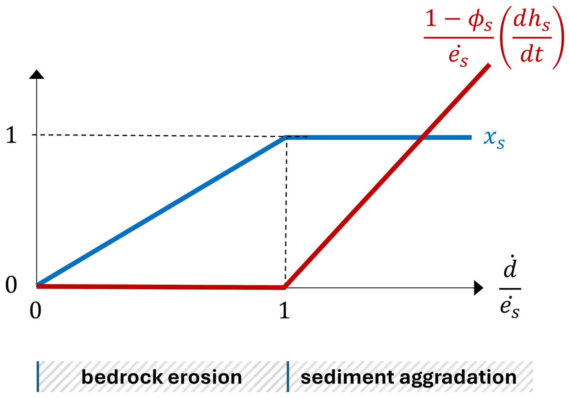
Figure 1 Diagram illustrating the transition from a system in which bedrock abrasion is possible (x_s<1) to a system in which it is not (x_s≥1). The evolution of the partitioning coefficient x_s is shown in blue as a function of the ratio of deposition rate to erosion rate. In red is the evolution of the aggradation rate normalized by the erosion rate as a function of the same ratio.

For a stationary solution, this yields an equation for the river load q_s:

$$\begin{array}{}\text{(13)}& {\displaystyle \frac{\mathrm{d}{q}_{\mathrm{s}}}{\mathrm{d}x}}={\dot{e}}_{\mathrm{b}}-{\displaystyle \frac{{\dot{e}}_{\mathrm{b}}}{{\dot{e}}_{\mathrm{s}}}}\dot{d}={\dot{e}}_{\mathrm{b}}-{\displaystyle \frac{{\dot{e}}_{\mathrm{b}}}{{\dot{e}}_{\mathrm{s}}}}{\displaystyle \frac{q_{\mathrm{s}}}{\mathit{\xi }}}\end{array}$$

Note that this Eq. (13) is similar to Eq. (3) but with an apparent transport length ${\mathit{\xi }}_{\mathrm{b}}=\frac{{\dot{e}}_{\mathrm{s}}}{{\dot{e}}_{\mathrm{b}}}\mathit{\xi }$.

The first end-member case is ${\dot{e}}_{\mathrm{b}}\to \mathrm{0}$, i.e., when the bedrock is not erodible. Then the transport length goes to infinity and Eq. (13) behaves as a detachment-limited equation, reflecting the fact that the sediment is constantly swept over the non-erodible bedrock.

In the general case ${\dot{e}}_{\mathrm{b}}>\mathrm{0}$, Eq. (13) can be written by substituting $q_{\mathrm{s}}^{\mathrm{\infty }}$ (Eq. 4) to ${\dot{e}}_{\mathrm{s}}$:

$$\begin{array}{}\text{(14)}& {\displaystyle \frac{\mathrm{d}{q}_{\mathrm{s}}}{\mathrm{d}x}}={\displaystyle \frac{\mathit{\alpha }{q}_{\mathrm{s}}}{\mathit{\xi }}}\left(\mathrm{1}-{\displaystyle \frac{q_{\mathrm{s}}}{q_{\mathrm{s}}^{\mathrm{\infty }}}}\right)\end{array}$$

With dimensionless variables, $q_{\mathrm{s}}^{\ast }=q_{\mathrm{s}}/q_{\mathrm{s}}^{\mathrm{\infty }}$ and $X^{\ast }=\mathit{\alpha }x/\mathit{\xi }$, Eq. (14) is written as:

$$\begin{array}{}\text{(15)}& {\displaystyle \frac{\mathrm{d}{q}_{\mathrm{s}}^{\ast }}{\mathrm{d}{X}^{\ast }}}=q_{\mathrm{s}}^{\ast }-{q_{\mathrm{s}}^{\ast }}^{\mathrm{2}}\end{array}$$

The equation is different from Eq. (6) and, above all, the characteristic scale ${\mathit{\xi }}_{\mathrm{b}}=\frac{\mathit{\xi }}{\mathit{\alpha }}$ is likely much larger than the bedload transfer length ξ. The general solution to Eq. (15) is:

$$\begin{array}{}\text{(16)}& {\left[\ln {\displaystyle \frac{q_{\mathrm{s}}^{\ast }}{\mathrm{1}-q_{\mathrm{s}}^{\ast }}}\right]}_{\mathrm{0}}^{x^{\ast \ast }}=X^{\ast }\end{array}$$

Posing $\mathit{\kappa }=\frac{q_{\mathrm{s}}^{\ast }\left(\mathrm{0}\right)}{\mathrm{1}-q_{\mathrm{s}}^{\ast }\left(\mathrm{0}\right)}\ast e^{X^{\ast }}$, we get the solution with $q_{\mathrm{s}}^{\ast }\left(\mathrm{0}\right)$ as the dimensionless sediment flux at $X^{\ast }=\mathrm{0}$:

$$\begin{array}{}\text{(17)}& q_{\mathrm{s}}^{\ast }={\displaystyle \frac{\mathit{\kappa }}{\mathrm{1}+\mathit{\kappa }}}={\displaystyle \frac{\mathrm{1}}{\mathrm{1}+\frac{\mathrm{1}-q_{\mathrm{s}}^{\ast }\left(\mathrm{0}\right)}{q_{\mathrm{s}}^{\ast }\left(\mathrm{0}\right)}{e}^{-X^{\ast }}}}\end{array}$$

In the limit $X^{\ast }\to \mathrm{\infty }$, we get $q_{\mathrm{s}}^{\ast }\to \mathrm{1}$, i.e., q_s tends to the transport capacity $q_{\mathrm{s}}^{\mathrm{\infty }}$. Solutions of Eq. (17) are shown in Fig. 2 for different values of the initial conditions $q_{\mathrm{s}}^{\ast }\left(\mathrm{0}\right)$. If there is no sediment at the inlet or if the bedload is in equilibrium, there is no change downstream. In the former case, the system cannot generate sediment along the stream; in the latter, there is no abrasion because the bedrock is covered by sediment (x_s=1). The distance to reach equilibrium varies as a function of the initial conditions.

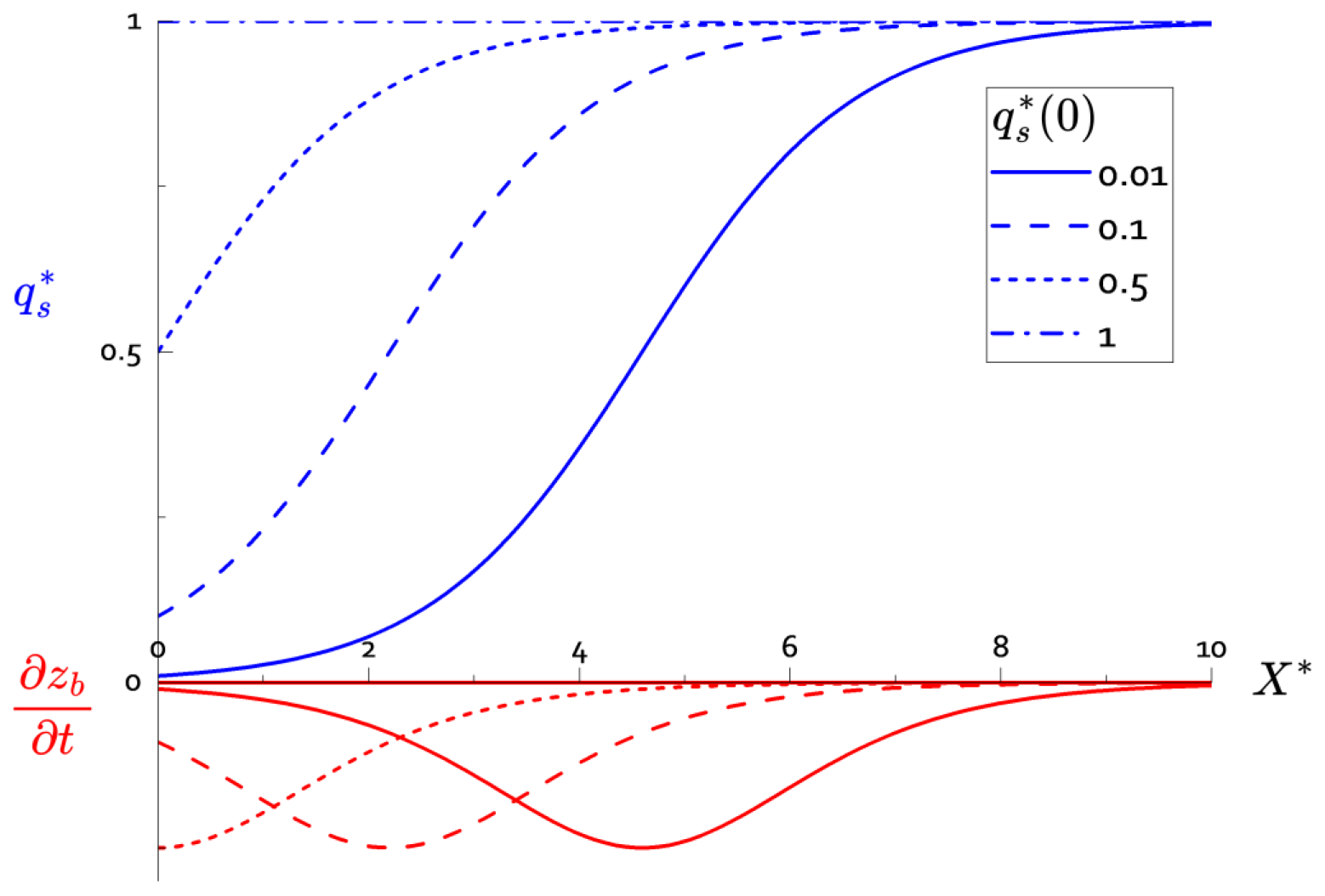
Figure 2 Plot of $q_{\mathrm{s}}^{\ast }=q_{\mathrm{s}}/q_{\mathrm{s}}^{\mathrm{\infty }}$ (in blue) and $\frac{\partial z_{\mathrm{b}}}{\partial t}$ (in red) as a function of the dimensionless distance ${x^{\prime }}^{\ast }=\mathit{\alpha }x/\mathit{\xi }$ for different values of the initial conditions $q_{\mathrm{s}}^{\ast }\left(\mathrm{0}\right)$ as indicated in the legend box.

The bedrock incision is given by Eq. (11c) with $x_{\mathrm{s}}=\frac{\dot{d}}{{\dot{e}}_{\mathrm{s}}}=\frac{q_{\mathrm{s}}}{\mathit{\xi }{\dot{e}}_{\mathrm{s}}}$, or by stating that the along-stream variation of q_s is balanced by the bedrock incision:

$$\left(\mathrm{1}-{\mathit{\varphi }}_{\mathrm{b}}\right){\displaystyle \frac{\partial z_{\mathrm{b}}}{\partial t}}=-{\displaystyle \frac{\mathrm{d}{q}_{\mathrm{s}}}{\mathrm{d}x}}={\displaystyle \frac{\mathit{\alpha }{q}_{\mathrm{s}}}{\mathit{\xi }}}\left(\mathrm{1}-{\displaystyle \frac{q_{\mathrm{s}}}{q_{\mathrm{s}}^{\mathrm{\infty }}}}\right)={\dot{e}}_{\mathrm{b}}\left(\mathrm{1}-{\displaystyle \frac{q_{\mathrm{s}}}{q_{\mathrm{s}}^{\mathrm{\infty }}}}\right)$$

This equation is equivalent to the bedrock abrasion Eq. (8) in SD2004, showing that the sediment/bedrock partitioning on which the model relies is equivalent to the empirical cover effect of SD2004. The additional equation of the coupled theory is Eq. (14) or Eq. (15).

The bedrock incision is maximal at the inflection point of the $q_{\mathrm{s}}^{\ast }$ curves (Fig. 2), i.e., at a distance for which $\frac{D^{\mathrm{2}}{q}_{\mathrm{s}}}{D{x}^{\mathrm{2}}}=\mathrm{0}$. This happens for x_M such that $q_{\mathrm{s}}^{\ast }\left(x_{\mathrm{M}}\right)=\mathrm{0.5}$ or $q_{\mathrm{s}}\left(x_{\mathrm{M}}\right)=\frac{q_{\mathrm{s}}^{\mathrm{\infty }}}{\mathrm{2}}$, giving:

$$\begin{array}{}\text{(18)}& x_{\mathrm{M}}={\displaystyle \frac{\mathit{\xi }}{\mathit{\alpha }}}\ln \left({\displaystyle \frac{\mathrm{1}-q_{\mathrm{s}}^{\ast }\left(\mathrm{0}\right)}{q_{\mathrm{s}}^{\ast }\left(\mathrm{0}\right)}}\right)\end{array}$$

2.3 Scaling of the bedrock/sediment coupled model with geomorphological parameters

The coupled theory basically depends on two main parameters: the bedrock coefficient α, which measures the ratio of bedrock abrasion flux to sediment load, and an apparent transport length ξ_b, referred to hereafter as the bedrock transport length. ξ_b controls the distance to the equilibrium state defined by a sediment flux at capacity and no more abrasion. These parameters depend on the flow characteristics, typically the transport stage $\mathit{\gamma }=\mathit{\tau }/{\mathit{\tau }}_{\mathrm{c}}$, the typical grain size D_s, and its density ρ_s (see Sect. 2). According to the scaling relationships given in SD2004 (see Appendix B) for w_i and ξ, the bedrock coefficient α scales as:

$$\begin{array}{}\text{(19)}& \mathit{\alpha }={\displaystyle \frac{{\mathit{\rho }}_{\mathrm{s}}{w}_{\mathrm{si}}^{\mathrm{2}}}{{\mathit{ϵ}}_{\mathrm{v}}}}=\mathrm{0.64}{\displaystyle \frac{R{\mathit{\rho }}_{\mathrm{s}}g{D}_{\mathrm{s}}}{{\mathit{ϵ}}_{\mathrm{v}}}}{\left(\mathit{\gamma }-\mathrm{1}\right)}^{\mathrm{0.36}}\end{array}$$

The transport length ξ_b scales as:

$$\begin{array}{}\text{(20)}& {\mathit{\xi }}_{\mathrm{b}}={\displaystyle \frac{\mathit{\xi }}{\mathit{\alpha }}}={\displaystyle \frac{\mathrm{100}}{\mathrm{8}}}\cdot {\displaystyle \frac{{\mathit{ϵ}}_{\mathrm{v}}}{{\mathit{\rho }}_{\mathrm{s}}Rg}}\cdot {\left(\mathit{\gamma }-\mathrm{1}\right)}^{\mathrm{0.52}}\end{array}$$

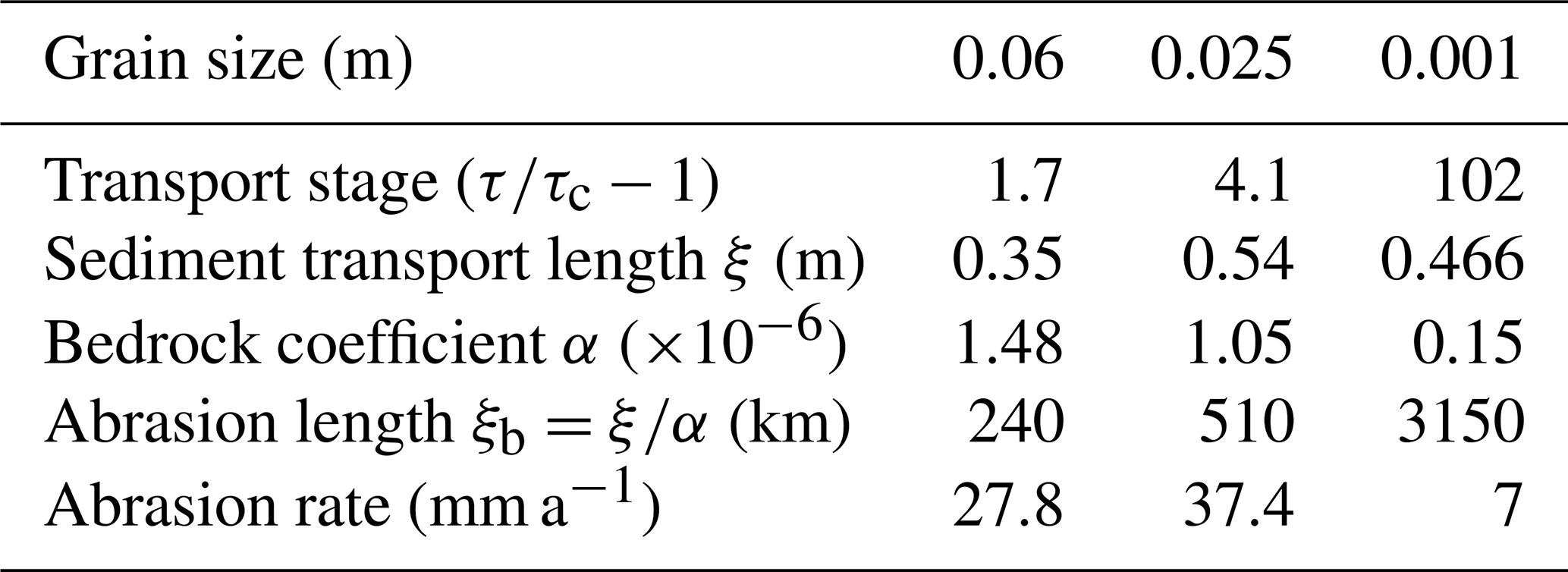
ξ_b is independent of the grain size diameter. α and ξ_b have been calculated for the emblematic case of the South Fork Eel River (Mendocino County, California) that is discussed in SD2004 and Lamb et al. (2008) for three grain sizes of 6 cm, 2.5 cm, and 1 mm and the corresponding transport stages of 1.7, 4 and 102. These values vary due to changes in τ_c. The bedrock coefficients, transport length ξ_b and erosion rates are given in the Table 1.

Table 1 Parameters of the abrasion model calculated for the South Fork Eel River in SD2004 for 3 different grain sizes.

3 Extension of the model to 2D fluxes with lateral erosion and deposition

3.1 Equations

To be used in landscape evolution models (see next sections), the model is extended to lateral erosion and deposition fluxes. In addition to being critical controls on channel widths (Croissant et al., 2017b; Davy et al., 2017; Nicholas, 2013), these lateral fluxes provide additional fluxes that modify the mass balance equations.

To our knowledge, there is no real consensus on the way to describe these additional fluxes. This concerns not only their parameterization, but also the correct description of the exchanges between the three stocks: bedrock, sediment cover and river load. We have opted for a very simple description of these lateral flows, and refer the reader to the literature to enrich the model if necessary (Fraccarollo and Rosatti, 2009; Fuller et al., 2016; Ikeda, 1982; Li et al., 2020; Li et al., 2021; Mishra et al., 2018; Parker, 1984a, b; Talmon et al., 1995; Yang et al., 2004; Sekine and Parker, 1992). In short, the main lateral processes are the erosion of lateral walls by fluid shear stress or particle impacts (abrasion) (Li et al., 2020; Li et al., 2021) and the lateral deflection of bedload over transverse slopes (Parker, 1984a, b; Talmon et al., 1995; Sekine and Parker, 1992; Ikeda, 1982).

We begin with a few definitions that may help the reader with the following developments. Lateral slopes refer to topographic slopes (not hydraulic slopes) and are denoted as ∇_lz. Lateral slopes are positive if the topography is sloping towards the considered point (${\mathrm{\nabla }}_{\mathrm{l}}^{+}z)$, otherwise they are negative (${\mathrm{\nabla }}_{\mathrm{l}}^{-}z)$. The superscript + (−, resp.) is attributed to neighbouring cells with higher (lower, resp.) topography: the cells are denoted N⁺ and N⁻, topography h⁺ and h⁻, bedload fluxes $q_{\mathrm{s}}^{+}$ and $q_{\mathrm{s}}^{-}$. Erosion processes are assumed to act on positive lateral slopes, and lateral bedload deflection on negative slopes.

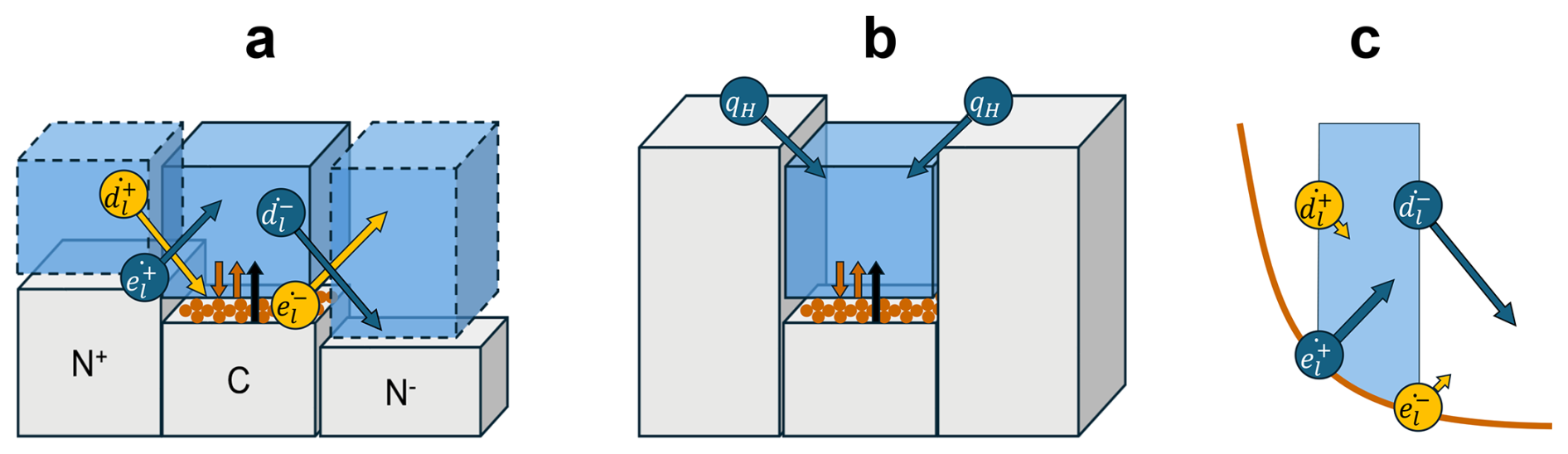
Figure 3 (a) Sketch showing the vertical and lateral fluxes in the vicinity of a cell C and the different compartments they link. ${\dot{e}}_{\mathrm{l}}$ and ${\dot{d}}_{\mathrm{l}}$ indicates the lateral erosion and deposition, respectively. The subscript + (−, resp.), indicates the fluxes from cells N⁺ (N⁻, resp.) with higher (lower, resp.) topography. The processes with the blue arrows (${\dot{e}}_{{\mathrm{l}}^{+}}$ and ${\dot{d}}_{{\mathrm{l}}^{-}}$) are controlled by the flow properties of C, specifically shear stress and bedload, and affect the bedload and topography of the adjacent cells N⁺ or N⁻. Conversely, the lateral fluxes indicated by yellow arrows are controlled by the flow properties of the adjacent cells and affect C. (b) The case of a river supplied with sediment from lateral hillslopes (see text). (c) The case where the main lateral fluxes are ${\dot{e}}_{{\mathrm{l}}^{+}}$ and ${\dot{d}}_{{\mathrm{l}}^{-}}$, i.e., those controlled by the flow characteristics of the cell.

Figure 3a shows how the lateral fluxes exchange sediment from the different compartments of the system, which are the bedload q_s, sediment cover h_s, bedrock topography h_b of the given cell, and the bedload q_sl and topography h_l of the neighbouring cells:

• ${\dot{e}}_{{\mathrm{l}}^{+}}$ is a flux between the topography of N⁺ and the bedload of C. It erodes N⁺ with the flow characteristics (i.e., shear stress) of C and the erodibility of N⁺;

• ${\dot{e}}_{{\mathrm{l}}^{-}}$ is a flux between the topography of C and the bedload of N⁻. It erodes C with the flow characteristics (shear stress) of N⁻ and the erodibility of C;

• ${\dot{d}}_{{\mathrm{l}}^{+}}$ is a flux between the bedload of N⁺ and the sediment cover of C. It depends on $q_{\mathrm{s}}^{+}$, the bedload of N⁺;

• ${\dot{d}}_{{\mathrm{l}}^{-}}$ is a flux between the bedload of C and the sediment cover of N⁻. It depends on q_s, the bedload of C;

We assume that lateral erosion is proportional to the lateral topographic slope. This hypothesis, which is supported by flume experiments (Inoue et al., 2025), is consistent with bed erosion perpendicular to topography, which links vertical and horizontal erosion through the topographic angle ${\mathrm{\nabla }}_{\mathrm{l}}^{+}z$. In the same way, we postulate that lateral deposition is in a ratio $\left|{\mathrm{\nabla }}_{\mathrm{l}}^{-}z\right|$ to basal deposition in line (Parker, 1984a, b; Talmon et al., 1995). If the lateral topographic gradients are small, this leads to simple expressions for the lateral erosion ${\dot{e}}_{\mathrm{l}}$ and lateral deposition ${\dot{d}}_{\mathrm{l}}$ as a function of the bedload erosion $\dot{e}$ (that can be either ${\dot{e}}_{\mathrm{s}}$ or ${\dot{e}}_{\mathrm{b}}$ depending on the nature of the neighbourhood) and bed deposition $\dot{d}$, respectively:

$$\begin{array}{}\text{(21)}& \left\{\begin{array}{l}{\dot{e}}_{{\mathrm{l}}^{+}}=k_{\mathrm{e}}{\mathrm{\nabla }}_{\mathrm{l}}^{+}z\dot{e}\\ {\dot{d}}_{{\mathrm{l}}^{-}}=k_{\mathrm{d}}\left|{\mathrm{\nabla }}_{\mathrm{l}}^{-}z\right|\dot{d}\end{array}\right.\end{array}$$

k_e and k_d are two dimensionless coefficients that contain mechanistic lateral processes that are beyond the simple geometric effect. For lateral erosion and deposition, a discussion on these coefficients can be found in different studies (Li et al., 2020, 2021; Parker, 1984a, b; Talmon et al., 1995) with typical values between 0 and 1. To keep expressions as simple as possible, we denote ${\mathit{\kappa }}_{\mathrm{e}}^{+}=k_{\mathrm{e}}{\mathrm{\nabla }}_{\mathrm{l}}^{+}z$, and ${\mathit{\kappa }}_{\mathrm{d}}^{-}=k_{\mathrm{d}}\left|{\mathrm{\nabla }}_{\mathrm{l}}^{-}z\right|$.

Mass balance equations similar to Eq. (11) can be written for the different compartments related to C in Fig. 3a:

$$\begin{array}{}\text{(22)}& \left\{\begin{array}{l}\frac{D\left(c_{\mathrm{s}}h\right)}{Dt}=x_{\mathrm{s}}{\dot{e}}_{\mathrm{s}}+\left(\mathrm{1}-x_{\mathrm{s}}\right){\dot{e}}_{\mathrm{b}}+{\dot{e}}_{{\mathrm{l}}^{+}}-\dot{d}-{\dot{d}}_{{\mathrm{l}}^{-}}\\ \left(\mathrm{1}-{\mathit{\varphi }}_{\mathrm{s}}\right)\frac{\partial h_{\mathrm{s}}}{\partial t}=-x_{\mathrm{s}}{\dot{e}}_{\mathrm{s}}-{\dot{e}}_{{\mathrm{l}}^{-}}+\dot{d}+{\dot{d}}_{{\mathrm{l}}^{+}}\\ \left(\mathrm{1}-{\mathit{\varphi }}_{\mathrm{b}}\right)\frac{\partial z_{\mathrm{b}}}{\partial t}=-\left(\mathrm{1}-x_{\mathrm{s}}\right){\dot{e}}_{\mathrm{b}}\end{array}\right.\end{array}$$

In addition to Eq. (22), the lateral neighbour N⁺is eroded by ${\dot{e}}_{{\mathrm{l}}^{+}}$ and the sediment cover of N⁻ increases by ${\dot{d}}_{{\mathrm{l}}^{-}}$.

To solve the equations, we use the same reasoning as in Sect. 2.2 for the case where the shear stress is large enough to remove all the sediment, i.e., $h_{\mathrm{s}}=\frac{\partial h_{\mathrm{s}}}{\partial t}=\mathrm{0}$ in Eq. (22).

$$\begin{array}{}\text{(23)}& {\displaystyle }{x}_{\mathrm{s}}={\displaystyle \frac{\mathrm{1}}{{\dot{e}}_{\mathrm{s}}}}\left(\dot{d}+{\dot{d}}_{{\mathrm{l}}^{+}}-{\dot{e}}_{{\mathrm{l}}^{-}}\right)\text{(24)}& {\displaystyle }\begin{array}{rl}{\displaystyle \frac{D\left(c_{\mathrm{s}}h\right)}{Dt}}=& {\dot{e}}_{\mathrm{b}}+{\dot{e}}_{{\mathrm{l}}^{+}}-{\displaystyle \frac{{\dot{e}}_{\mathrm{b}}}{{\dot{e}}_{\mathrm{s}}}}\dot{d}-{\dot{d}}_{{\mathrm{l}}^{-}}\\ & -\left(\mathrm{1}-{\displaystyle \frac{{\dot{e}}_{\mathrm{b}}}{{\dot{e}}_{\mathrm{s}}}}\right)\left({\dot{e}}_{{\mathrm{l}}^{-}}-{\dot{d}}_{{\mathrm{l}}^{+}}\right)\end{array}\end{array}$$

Using the expressions for lateral fluxes and vertical deposition in Eq. (21) and α as defined in Eq. (10), we obtain:

$$\begin{array}{}\text{(25)}& \begin{array}{rl}{\displaystyle \frac{D\left(c_{\mathrm{s}}h\right)}{Dt}}=& {\dot{e}}_{\mathrm{b}}\left(\mathrm{1}+{\mathit{\kappa }}_{\mathrm{e}}^{+}\right)-{\displaystyle \frac{q_{\mathrm{s}}}{\mathit{\xi }}}\left({\displaystyle \frac{{\dot{e}}_{\mathrm{b}}}{{\dot{e}}_{\mathrm{s}}}}+{\mathit{\kappa }}_{\mathrm{d}}^{-}\right)\\ & -\left(\mathrm{1}-\mathit{\alpha }\right)\left({\dot{e}}_{{\mathrm{l}}^{-}}-{\dot{d}}_{{\mathrm{l}}^{+}}\right)\end{array}\end{array}$$

The equation has even less of a trivial solution, since the last two terms ${\dot{e}}_{{\mathrm{l}}^{-}}$ and ${\dot{d}}_{{\mathrm{l}}^{+}}$ depend on the flow characteristics of the neighbours N⁺ and N⁻. The solution, where the lateral topographic gradients are very small, is similar to the 1D case. We discuss below two cases illustrated in Fig. 3a and b.

Note that bedrock erosion occurs only if ${\dot{e}}_{\mathrm{s}}>-{\dot{e}}_{{\mathrm{l}}^{-}}+\dot{d}+{\dot{d}}_{{\mathrm{l}}^{+}}$ (i.e., x_s<1 in the middle equation of Eq. 22). If this is not the case, depositional fluxes will overtake erosion fluxes and sediment will accumulate on the riverbed.

3.2 Example 1: bedrock incision with sediment supply from hillslopes

We illustrate the consequences of lateral flows on sediment/bedrock dynamics with the case of a river supplied with sediment by hillslopes (Fig. 3b). The question will be addressed at the river section scale, integrating flows across the width of the channel W. The sediment fluxes are in m³ s⁻¹ and denoted with capitals, e.g. the bedload flux is $Q_{\mathrm{s}}=W\ast q_{\mathrm{s}}$ and the transport capacity $Q_{\mathrm{s}}^{\mathrm{\infty }}=W\ast q_{\mathrm{s}}^{\mathrm{\infty }}$, the sediment erosion rate is ${\dot{E}}_{\mathrm{s}}=W{\dot{e}}_{\mathrm{s}}$, etc. The control parameter for this case is the total lateral sediment flux from hillslopes per unit of stream length q_H. q_H is assumed to be supplied directly to the bedload; the result would not be different if it supplies the sediment cover.

The stationary bedload flux equation $\left(\mathrm{i}.\mathrm{e}.,\frac{D\left(c_{\mathrm{s}}h\right)}{Dt}=\frac{\mathrm{d}{q}_{\mathrm{s}}}{\mathrm{d}x}\right)$ is similar to Eq. (14) but with the source term q_H equivalent to ${\dot{e}}_{{\mathrm{l}}^{+}}$ in Eq. (25):

$$\begin{array}{}\text{(26)}& {\displaystyle \frac{\mathrm{d}{Q}_{\mathrm{s}}}{\mathrm{d}x}}=\mathit{\alpha }{\displaystyle \frac{Q_{\mathrm{s}}}{\mathit{\xi }}}\left(\mathrm{1}-{\displaystyle \frac{Q_{\mathrm{s}}}{Q_{\mathrm{s}}^{\mathrm{\infty }}}}\right)+q_{\mathrm{H}}\end{array}$$

The equation simplifies by using the same dimensionless variables as in the 1D case: $X^{\ast }=\frac{\mathit{\alpha }x}{\mathit{\xi }}$ and $Q_{\mathrm{s}}^{\ast }=Q_{\mathrm{s}}/Q_{\mathrm{s}}^{\mathrm{\infty }}$:

$$\begin{array}{}\text{(27)}& {\displaystyle \frac{\mathrm{d}{Q}_{\mathrm{s}}^{\ast }}{\mathrm{d}{X}^{\ast }}}=Q_{\mathrm{s}}^{\ast }-{Q_{\mathrm{s}}^{\ast }}^{\mathrm{2}}+Q_{\mathrm{H}}^{\ast }\end{array}$$

Where $Q_{\mathrm{H}}^{\ast }=\frac{\mathit{\xi }{q}_{\mathrm{H}}}{\mathit{\alpha }{Q}_{\mathrm{s}}^{\mathrm{\infty }}}$.

The stationary solution is:

$$\begin{array}{}\text{(28)}& Q_{\mathrm{s},\mathrm{stat}}^{\ast }={\displaystyle \frac{\mathrm{1}+\sqrt{\mathrm{1}+\mathrm{4}{Q}_{\mathrm{H}}^{\ast }}}{\mathrm{2}}}\end{array}$$

Equation (26) is a simple Riccati's equation that has an analytical solution. With ${\mathit{\kappa }}^{\prime }=\frac{\sqrt{\mathrm{1}+\mathrm{4}{Q}_{\mathrm{H}}^{\ast }}}{\mathrm{2}}$ and $Q_{\mathrm{s}}^{\ast }\left(\mathrm{0}\right)$ the value of $Q_{\mathrm{s}}^{\ast }$ at $x^{\ast \ast }=\mathrm{0}$, the solution is written as:

$$\begin{array}{}\text{(29)}& Q_{\mathrm{s}}^{\ast }={\mathit{\kappa }}^{\prime }\tanh \left({\mathit{\kappa }}^{\prime }{X}^{\ast }+\mathrm{arctanh}\left({\displaystyle \frac{Q_{\mathrm{s}}^{\ast }\left(\mathrm{0}\right)-\mathrm{0.5}}{{\mathit{\kappa }}^{\prime }}}\right)\right)+\mathrm{0.5}\end{array}$$

An example of the solution for different values of $Q_{\mathrm{H}}^{\ast }$ is shown in Fig. 4 with two different bedload values $Q_{\mathrm{s}}^{\ast }\left(\mathrm{0}\right)$ at the inlet: 0 and 0.1. The distance to reach equilibrium depends on the largest value between $Q_{\mathrm{s}}^{\ast }\left(\mathrm{0}\right)$ and $Q_{\mathrm{H}}^{\ast }$, while the upstream and downstream conditions depend only on $Q_{\mathrm{s}}^{\ast }\left(\mathrm{0}\right)$ and $Q_{\mathrm{H}}^{\ast }$, respectively.

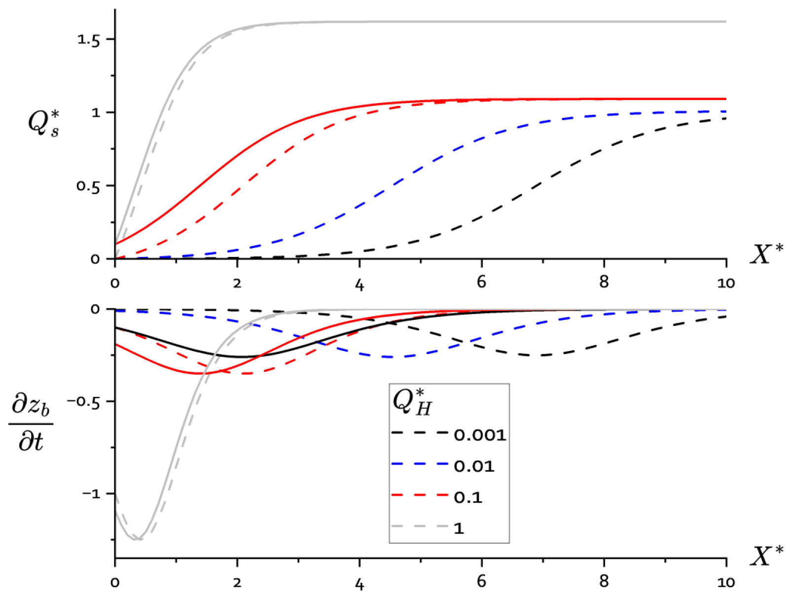
Figure 4 Top: Plot of $q_{\mathrm{s}}^{\ast }=q_{\mathrm{s}}/q_{\mathrm{s}}^{\mathrm{\infty }}$ as a function of the dimensionless distance ${x^{\prime }}^{\ast }=\mathit{\alpha }x/\mathit{\xi }$ for different values of the hillslope supply parameter $Q_{\mathrm{H}}^{\ast }$ (colours as indicated in the legend box) and $Q_{\mathrm{s}}^{\ast }\left(\mathrm{0}\right)$. The dashed lines are plotted for $Q_{\mathrm{s}}^{\ast }\left(\mathrm{0}\right)=\mathrm{0}$; the solid lines are plotted for $Q_{\mathrm{s}}^{\ast }\left(\mathrm{0}\right)=\mathrm{1}$. Bottom: plot of the bedrock erosion rate as a function of ${x^{\prime }}^{\ast }$. The legends are the same as for the top graph.

Since the sediment cover does not participate in the mass balance, the bedrock incision is the counterpart of the variation of Q_s with distance: $(\mathrm{1}-{\mathit{\varphi }}_{\mathrm{b}})\frac{\partial z_{\mathrm{b}}}{\partial t}=-\frac{D{q}_{\mathrm{s}}}{Dx}$. It first increases up to the inflexion point of $Q_{\mathrm{s}}^{\ast }$ and then decreases to 0 as the bedload gets closer to the stationary plateau. The maximum is reached at a distance x_M where $\frac{D^{\mathrm{2}}{q}_{\mathrm{s}}}{D{x}^{\mathrm{2}}}=\mathrm{0}$ $\left(\frac{D^{\mathrm{2}}{Q}_{\mathrm{s}}}{D{x}^{\mathrm{2}}}=\mathrm{0}\mathrm{if}\mathrm{the}\mathrm{river}\mathrm{width}\mathrm{remains}\mathrm{constant}\right)$. Considering Eq. (27), $Q_{\mathrm{s}}^{\ast }\left(x_{\mathrm{M}}\right)$ is solution of the polynomial equation $Q_{\mathrm{H}}^{\ast }+Q_{\mathrm{s}}^{\ast }(\mathrm{1}-\mathrm{2}{Q}_{\mathrm{H}}^{\ast })-\mathrm{3}{Q_{\mathrm{s}}^{\ast }}^{\mathrm{2}}-\mathrm{2}{Q_{\mathrm{s}}^{\ast }}^{\mathrm{3}}=\mathrm{0}$, which can be solved numerically.

To evaluate how large $Q_{\mathrm{H}}^{\ast }$ can be under natural conditions, we calculate it for the South Fork Eel River case developed in Sect. 2.3. As q_H was not considered in SD2004, we make the reasonable assumption that hillslopes erode at a rate U of the order of mm yr⁻¹, and q_H is the total sediment flux when integrating U over the hillslope length L_H. This leads to $q_{\mathrm{H}}\sim \mathrm{3}\times {\mathrm{10}}^{-\mathrm{8}}$ m² s⁻¹ for U=1 mm yr⁻¹ and L_H=1 km. For the 3 studied grain sizes of 6 cm, 2.5 cm, and 1 mm, the values of $Q_{\mathrm{H}}^{\ast }$ are $\mathrm{5}\times {\mathrm{10}}^{-\mathrm{4}}$, 10⁻³ and $\mathrm{6}\times {\mathrm{10}}^{-\mathrm{3}}$.

To conclude on this part, the transport capacity – if defined as the sediment load at which erosion and deposition rates are in equilibrium – depends on the hillslope supply. It is no longer an intrinsic value that depends solely on the river erosion and transport capacities. The deviation from the theoretical transport capacity defined by $Q_{\mathrm{s}}^{\mathrm{\infty }}=W\mathit{\xi }{\dot{e}}_{\mathrm{s}}$ depends on the dimensionless hillslope supply $Q_{\mathrm{H}}^{\ast }=\frac{\mathit{\xi }}{\mathit{\alpha }}\frac{q_{\mathrm{H}}}{Q_{\mathrm{s}}^{\mathrm{\infty }}}$, which increases as grain size decreases. In the case of the South Fork Eel River, the effect is significant only for hillslope erosion rates of the order of m yr⁻¹. The stationary bedload regime depends on $Q_{\mathrm{H}}^{\ast }$ and on the initial bedload fluxes. The characteristic distance to reach it is the same as for the 1D case, i.e., $\frac{\mathit{\xi }}{\mathit{\alpha }}$, where ξ is the transport length and α is the dimensionless bedrock coefficient. Depending on $Q_{\mathrm{H}}^{\ast }$ and $Q_{\mathrm{s}}^{\ast }\left(\mathrm{0}\right)$, this distance can be several times this characteristic distance.

3.3 Example 2: sediment transfer from banks to river centre

In the general case, the solution of Eq. (25) is not trivial and depends on the characteristics of the neighbouring cells. Approximate solutions can be obtained either by relating the erosion and deposition fluxes in the neighbours to those of the cell, or by keeping the fluxes in Eq. (25) that depend only on the cell characteristics, i.e., all the terms on the right-hand side except ${\dot{e}}_{{\mathrm{l}}^{-}}$ and ${\dot{d}}_{{\mathrm{l}}^{+}}$. We develop only the latter, which corresponds to the case illustrated in Fig. 3c, which could correspond to streamlines close to the riverbanks.

This leads to an expression that is slightly different from the 1D Eq. (14). If we replace ${\dot{e}}_{\mathrm{b}}$ by $\frac{\mathit{\alpha }{q}_{\mathrm{s}}}{\mathit{\xi }}$ and $\frac{{\dot{e}}_{\mathrm{b}}}{{\dot{e}}_{\mathrm{s}}}$ by $\mathit{\alpha }\frac{q_{\mathrm{s}}}{q_{\mathrm{s}}^{\mathrm{\infty }}}$, Eq. (25) becomes:

$$\begin{array}{}\text{(30)}& {\displaystyle \frac{\mathrm{d}{q}_{\mathrm{s}}}{\mathrm{d}x}}=\mathit{\alpha }{\displaystyle \frac{q_{\mathrm{s}}}{\mathit{\xi }}}\left(\mathrm{1}+{\mathit{\kappa }}_{\mathrm{e}}^{+}-{\displaystyle \frac{{\mathit{\kappa }}_{\mathrm{d}}^{-}}{\mathit{\alpha }}}-{\displaystyle \frac{q_{\mathrm{s}}}{q_{\mathrm{s}}^{\mathrm{\infty }}}}\right)\end{array}$$

The coefficients α, ${\mathit{\kappa }}_{\mathrm{e}}^{+}$, ${\mathit{\kappa }}_{\mathrm{d}}^{-}$ are significantly smaller than 1. The solutions of Eq. (30) depend on whether $\frac{{\mathit{\kappa }}_{\mathrm{d}}^{-}}{\mathit{\alpha }}$ is larger or smaller than $\mathrm{1}+{\mathit{\kappa }}_{\mathrm{e}}^{+}$. We pose $\mathit{\beta }=\mathrm{1}+{\mathit{\kappa }}_{\mathrm{e}}^{+}-\frac{{\mathit{\kappa }}_{\mathrm{d}}^{-}}{\mathit{\alpha }}$ and ${q_{\mathrm{s}}^{\prime }}^{\mathrm{\infty }}=\mathit{\beta }{q}_{\mathrm{s}}^{\mathrm{\infty }}$, the equation is written as:

$$\begin{array}{}\text{(31)}& {\displaystyle \frac{\mathrm{d}{q}_{\mathrm{s}}}{\mathrm{d}x}}=\mathit{\alpha }\mathit{\beta }{\displaystyle \frac{q_{\mathrm{s}}}{\mathit{\xi }}}\left(\mathrm{1}-{\displaystyle \frac{q_{\mathrm{s}}}{{q_{\mathrm{s}}^{\prime }}^{\mathrm{\infty }}}}\right)\end{array}$$

The equation is similar to Eq. (14) but with αβ instead of α and $\mathit{\beta }{q}_{\mathrm{s}}^{\mathrm{\infty }}$ instead of $q_{\mathrm{s}}^{\mathrm{\infty }}$. An important difference is that β is not necessarily positive, with three possible cases:

• If β>0, the solution is similar to Eq. (17) except that the limit for x→∞ is now: $q_{\mathrm{s}}\to \mathit{\beta }{q}_{\mathrm{s}}^{\mathrm{\infty }}$, which can be smaller or larger than $q_{\mathrm{s}}^{\mathrm{\infty }}$, and the characteristic distance is ${\mathit{\xi }}_{\mathrm{b}}^{\prime }=\frac{{\mathit{\xi }}_{\mathrm{b}}}{\mathit{\beta }}=\frac{\mathit{\xi }}{\mathit{\alpha }\mathit{\beta }}$.

• If β<0, $\frac{\mathrm{d}{q}_{\mathrm{s}}}{\mathrm{d}x}$ is always negative, and the stationary solution is q_s→0. q_s exponentially decreases to 0 with a characteristic distance ${\mathit{\xi }}_{\mathrm{b}}^{\prime }=\frac{{\mathit{\xi }}_{\mathrm{b}}}{\left|\mathit{\beta }\right|}=\frac{\mathit{\xi }}{\mathit{\alpha }\left|\mathit{\beta }\right|}$

• If β=0, q_s tends to 0 as x⁻¹.

The consequence of lateral fluxes is that they modify the transport capacity close to the riverbanks, as well as the distance to reach it compared to the of the river cross-section.

4 Numerical simulations

4.1 Implementation

The abrasion equation (25) has been implemented in the numerical platform RIVER.lab/eros, which is described in detail by Davy and Lague (2009) and Davy et al. (2017). This method is based on the displacement of small volumes of water containing sediments, which are referred to as “precipitons” hereafter. In contrast to the stream power incision model, in which abrasion (as well as plucking and attrition) has been introduced (Gabel et al., 2024), this model provides a more complete description of hydrodynamics – the shallow water equation without inertia – which enables the river width to emerge as a property of the simulation rather than being defined by a parametric equation.

Precipitons are introduced at the inlet boundary at a rate $Q_{\mathrm{in}}/V_{\mathrm{p}}$, where Q_in is the total inflow rate and V_p is the water volume of a precipiton. The volume of sediment carried is c_sV_p. The precipitons then move along the grid following the hydraulic gradient, until they reach an outlet.

During each elementary displacement, precipitons first solve the hydrodynamic and then the geomorphological equations. Hydrodynamics involves calculating the water depth by solving the shallow water equations without inertia, balancing basal friction and gravity forces (Davy et al., 2017; Hocini et al., 2021). All inertial effects, such as those associated with secondary flows, are thus not considered (see discussion of potential effects in Inoue et al., 2025). Water discharge is given by the flux of precipitons passing through a given cell. The shear stress τ is equal to ρghs with s the hydraulic slope or to ρg(nq)^0.6s^0.3, where q=uh is the flow per unit width and n is the Manning friction coefficient.

Geomorphological evolution involves solving Eq. (22) to calculate the volume of sediment exchanged between the running precipiton and the bedrock and alluvial covers at the grid point and its lateral neighbours. First, variations of c_s are calculated by solving the exchange Eq. (25) under the assumption that erosion fluxes remain constant throughout each grid step, Then, the other terms in the mass balance equations (basal and lateral alluvial covers, and basal and lateral bedrock topographies) are updated according to Eq. (22). The erosion and deposition fluxes are those illustrated in Fig. 3. For sediments, the erosion rate is given by the Meyer-Peter&Müller equation (MPM) (Meyer-Peter and Müller, 1948). Bedrock incision by abrasion is solved using Eq. (25), whose main parameters (α and $\mathit{\xi }/\mathit{\alpha }$) depend on the abrasion parameter ϵ_v.

During each passage through a grid cell, the precipiton removes any sediment layer, including that deposited from neighbouring precipitons (e.g., ${\dot{d}}_{\mathrm{l}}^{+}$ in Fig. 3), before eroding the bedrock. The erosion time is thus partitioned between sediment erosion using the MPM equation until the basement is no longer covered by sediment, and the basement equation (25) thereafter. The precipiton calculates the lateral fluxes ${\dot{d}}_{\mathrm{l}}^{-}$ and ${\dot{e}}_{\mathrm{l}}^{+}$; the two other fluxes (${\dot{d}}_{\mathrm{l}}^{+}$ and ${\dot{e}}_{\mathrm{l}}^{-}$) are calculated by neighbouring precipitons.

The time step of the simulation is adapted to manage the fastest process, i.e. sediment transport. But, for a typical abrasion parameter of 1 GPa (Sklar and Dietrich, 2012; Sklar and Dietrich, 2004), abrasion rates are 10⁶ times slower than sediment erosion, which precludes the possibility of calculating significant abrasion erosion in a reasonable computation time. However, if sediment flows are at quasi-steady state with a slowly evolving bedrock, it is possible to extrapolate the result of a simulation to other abrasion parameters, provided that the times are scaled in inverse proportion to the abrasion parameter. Whilst the testing of the steady-state hypothesis is beyond the scope of the present study, insights are provided by way of simulations involving two abrasion parameters that are markedly different.

4.2 Simulation of the Rheinfall at Schaffhausen

This example illustrates how the model behaves under natural conditions. We chose the Rheinfall in Schaffhausen, a prominent 20 m-high knickpoint, to show how this iconic knickpoint will be eliminated when coarse debris is available. Differential erodibilities may play an important role as the area is located between the northern rim of the easily erodible Molasse sediments and the hard-to-erode Malm limestones that build the actual Rheinfall (Hofmann, 1987). The area has been laterally mobile previously, subsequent clogging of riverbeds by sediment and lateral shifts in stream location was probably associated with large foreland glaciations. The Rheinfall developed at its present position about 15 000 years ago and exhibits only minor mechanical erosion.

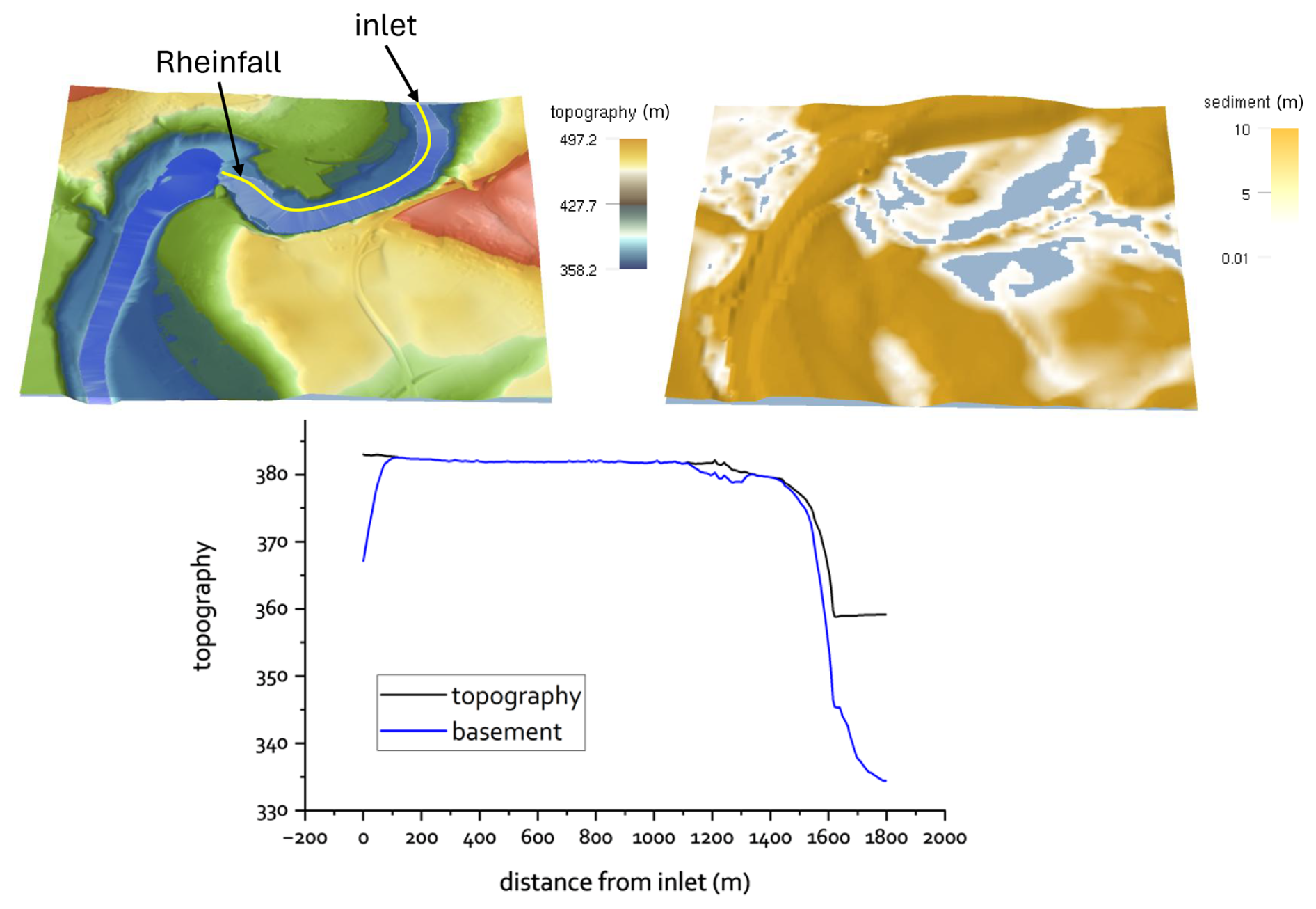
Figure 5 Top row, topography (left) and sediment (right) maps of the studied area. The units are meters. Bottom row, topography and bedrock profiles from inlet to the bottom of the Rheinfall knickpoint (yellow line in top row left).

Model topography is a lidar-derived DEM that is made available for entire Switzerland from Swisstopo (https://www.swisstopo.admin.ch/en/height-model-swissalti3d, last access: December 2023). The data are available with 0.5 and 2 m spatial ground resolution. For simulations, we use a 6 m resolution grid and we simulated erosion of the Rhine with boundary conditions set at approximately 1 km upstream of the waterfall (Fig. 5). The initial sediment cover has been estimated from Pietsch and Jordan (2014). Except for a few patches of sediment, the bedrock is exposed across the entire current bed of the Rhine in the area upstream of the waterfall.

For this test, the boundary condition at the model inlet is a flow rate of 370 m³ s⁻¹, which is applied to the inlet Rhine section. The Manning friction coefficient is 0.03 in SI units. The sediment grain size is 2.5 mm, and the sediment concentration is varied (Davy et al., 2017; Hocini et al., 2021). The simulation time is the total duration of these high-flow events, expressed in years. In reality, these events occur sporadically, so the actual time should be longer.

4.2.1 Case of a sediment-like basement

The difference between a sediment-like equation and the novel abrasion equation is illustrated by running two simulations. In the first simulation, the basement erosion equation is the same as the sediment equation and has the same erodibility. In the second simulation, the erodibility is 1000 times smaller. The input sediment concentration in volume is 10⁻³.

Figure 6 Simulations with a basement equation similar to the sediment equation and an input sediment concentration of 10⁻³. The blue colour indicates water depth. Left: Erodibility for the basement is the same as for the sediment. Right: erodibility is 1000 times lower than in the left case.

In both cases, the basement erodes towards a convex profile whose shape corresponds to the stationary solution of the simulated advective-diffusion equation (Fig. 6). The shape of the profile and the time taken to reach the stationary solution depend on the erodibility of the basement. In both cases, the knickpoint profile becomes smoother with time, highlighting the diffusive nature of the erosion process, which is consistent with the low values of the sediment transport length. For the simulation parameters, the knickpoint shape is stationary after a few years.

A difference in erodibility between the bedrock and the sediments leads to a drastic reduction in the width of the river, forming a narrow canyon. As expected, the erosion time scales with the ratio of basement to sediment erodibility, i.e. 1000 times slower in this simulation than in the previous one.

4.2.2 Abrasion case

We have carried out a series of numerical simulations of the effect of abrasion on river erosion. We vary two parameters: the abrasion parameter ϵ_v which is likely to control erosion rates by abrasion, and the flux of sediments, which controls tool and cover effects.

For reasons of computational time outlined in Sect. 4.1, we carry out two series of numerical experiments, the first with an abrasion parameter ϵ_v of 10⁴ Pa, and the second with 10⁵ Pa. The objective is to visualize the erosion patterns and to estimate how erosion rates scale with ϵ_v. For each series, we vary the input sediment concentration from 10⁻⁵ to 10⁻².

The lateral erosion parameters are equal to 1 for either sediment or bedrock erosion.

Erosion patterns

We illustrate the erosion patterns using the abrasion parameters, ϵ_v=10⁴ Pa and $c_{\mathrm{s}}^{\mathrm{in}}={\mathrm{10}}^{-\mathrm{4}}$ (Fig. 7). First, two canyons extend upstream from the base of the Schaffhausen knickpoint, each measuring approximately 30 to 50 m in width during the initial stages. After 1000 years, the southern canyon is cut off from its water supply by the northern canyon, which continues to advance upstream and widen. Ultimately, the northern canyon reaches a downstream width of about 80 m. The evolution of the canyon profile and width is shown in Fig. 8.

Figure 7 Simulations of the baseline model. Plan views of a simulation at 6 different times for the baseline model with ϵ_v=10⁴ Pa and $c_{\mathrm{s}}^{\mathrm{in}}={\mathrm{10}}^{-\mathrm{4}}$ with the same colour scales as in Fig. 6.

Figure 8 Temporal evolution of river profile in baseline model simulation. Left: canyon profile at different times for the simulation shown in Fig. 7. Right: canyon width at different times in the section indicated by the yellow line on the first plan view of Fig. 7. The dashed line is the altitude of the base of the Schaffhausen fall.

The knickpoint shape is maintained in the canyons throughout their upstream propagation, exhibiting a steepest slope of 10 % (Fig. 8, left). Both downstream and upstream of the knickpoints, the topographic slopes are less than 0.1 %. The analysis of canyon width over time is illustrated in the right graph in Fig. 8. Two stages in the evolution of canyon width can be identified. In the first stage (up to about 1000 years for the cross-section indicated by the yellow line in Fig. 7), the canyon incises in the bedrock with a V-shape and constant lateral slopes. Once the canyon bottom reaches a base level, incision ceases, and the width increases significantly, ultimately reaching 80 m.

Effect of input sediment concentration

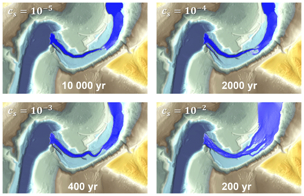
The sediment flux is a critical parameter in the erosion pattern since it controls the erosion rate by abrasion. Figure 9 shows a plan view of the canyon at one stage of its development for 4 runs with inlet sediment concentrations c_s of 10⁻⁵, 10⁻⁴, 10⁻³ and 10⁻². The inlet sediment flux is $Q_{\mathrm{s}}=c_{\mathrm{s}}\ast Q$, where Q is the total discharge at the inlet. Figure 10 shows profile evolutions corresponding to the 4 runs presented in Fig. 9 and a run with no sediment flux at the inlet. For the latter (c_s=0), the knickpoint erodes at the very first stage due to the mobilization of the preexisting sediment patches on the riverbed, but once this source of sediment is depleted, the basement is no longer eroded confirming the model's ability to simulate abrasion as a sediment-driven process.

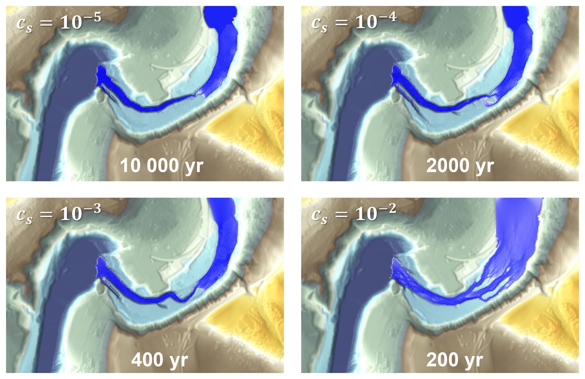
Figure 9 Simulation results varying sediment concentration c_s. Plan view of 4 runs with ${\mathit{ϵ}}_{\mathrm{v}}={\mathrm{10}}^{-\mathrm{4}}$ and input sediment concentrations of 10⁻⁵ at 10 000 years (top left), 10⁻⁴ at 2000 years (top right), 10⁻³ at 400 years (bottom left), and 10⁻² at 200 years (bottom right). The same colour scales as in Fig. 6.

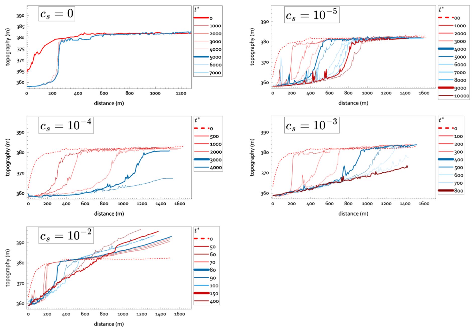
Figure 10 Temporal evolution of river long profile in simulation with varying sediment concentration c_s. Canyon profile at different times for the simulation shown in Fig. 9.

For all the runs, there is no sediment on the basement except for moving patches, visible for instance in the last run shown in Fig. 9 ($c_{\mathrm{s}}={\mathrm{10}}^{-\mathrm{2}}$).

The inlet sediment flux has two main effects: an increase of the knickpoint erosion rate with c_s, and along stream profiles that vary with c_s (Fig. 10). The former is not surprising since the erosion rate is driven by sediment concentration. We provide a quantitative analysis of erosion rates in a later section. The erosion profile preserves the knickpoint shape when c_s is less than 10⁻³ with a small stream slope downstream of the knickpoint. With increasing c_s, the river downstream of the knickpoint steepens, attaining slopes up to 3 %. These steep slopes reflect the river steepness required to evacuate the layer of sediment that is continuously deposited by the high concentrations.

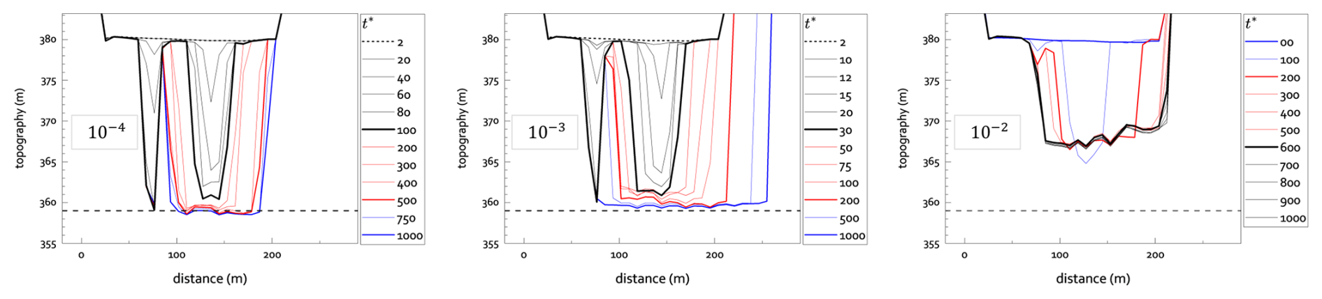
Figure 11 Temporal evolution of river cross section in simulation with varying sediment concentration. Evolution of the canyon section shown by the yellow line in Fig. 7 for 3 runs corresponding to inlet sediment concentration of 10⁻⁴, 10⁻³, and 10⁻².

The evolution of the canyon cross profile is shown in Fig. 11 with a first stage of vertical incision followed by a widening as already described in the previous section.

Scaling with the abrasion parameter

A series of runs have been carried out with an abrasion parameter ${\mathit{ϵ}}_{\mathrm{v}}=\mathrm{3.5}\times {\mathrm{10}}^{\mathrm{4}}$ Pa, significantly larger than in the previous set. The objective is to analyze how the resulting erosion pattern and rates scale with ϵ_v. The results are presented in Fig. 12 for different values of the input sediment concentration c_s. The propagation of the canyon can be slightly more erratic than in the previous runs with ${\mathit{ϵ}}_{\mathrm{v}}={\mathrm{10}}^{+\mathrm{4}}$ Pa. This behaviour reflects a highly non-linear general pattern, with a complex coupling between hydraulics, sediment transport and abrasion.

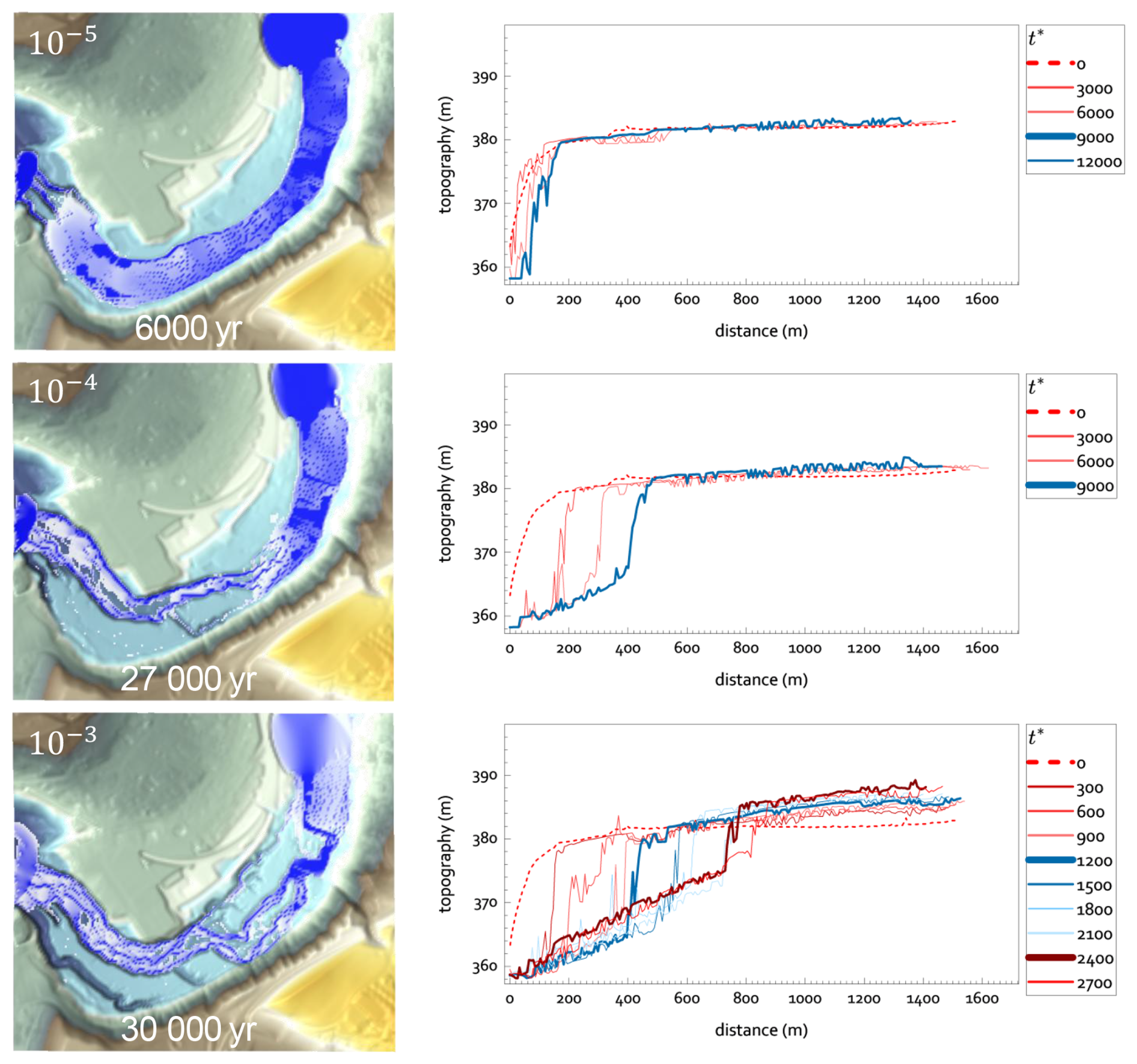
Figure 12 Simulation results with ${\mathit{ϵ}}_{\mathrm{v}}=\mathrm{35}\times {\mathrm{10}}^{\mathrm{4}}$ Pa. Left column: plan view of three runs with input sediment concentrations of 10⁻⁵ at 2300 years (top left), 10⁻⁴ at 27 000 years (middle left), and 10⁻³ at 30 000 years (bottom left). The scale is the same as for Fig. 6. Right column: the evolution of the along-stream canyon profile for the corresponding run in the same row.

Summary of the erosion rates

Figure 13 summarizes the average knickpoint retreat rates calculated from the evolution of the canyon profile. Note that these rates can vary over time, depending on the position and width of the canyon. Also, two simulations with the same parameters but different random numbers used to generate precipitons can produce slightly different results due to the unstable behaviour of the system.

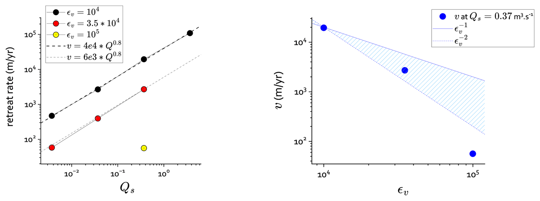
Figure 13 Left: Knickpoint retreat rates in m yr⁻¹ as a function of the inlet sediment flux for the three values of the abrasion parameter ϵ_v. The symbols are indicated in the graph legend. The thick and thin dashed line are the fits v(Q_s) for ϵ_v=10⁴ and 35×10⁴ Pa. Right: evolution of v with the abrasion parameter ϵ_v at Q_s=37 m³ s⁻¹. The blue lines indicate a dependency on ${\mathit{ϵ}}_{\mathrm{v}}^{-\mathrm{1}}$ (solid line) and ${\mathit{ϵ}}_{\mathrm{v}}^{-\mathrm{2}}$ (dashed line).

For ϵ_v=10⁴ Pa, the knickpoint retreats at rates v increase with the sediment concentration c_s, and thus with the total sediment flux Q_s=c_sQ, as $v=\mathrm{4}\times {\mathrm{10}}^{\mathrm{4}}{Q}_{\mathrm{s}}^{\mathrm{0.8}}$ (Fig. 13, left). Although the knickpoint height tends to decrease when increasing c_s and time, the retreat rate does not depart from this scaling relationship. The fact that the relationship is less than linear – i.e., that the retreat is relatively less efficient at high Q_s – may be due to different responses in canyon width and along-stream profiles.

For ${\mathit{ϵ}}_{\mathrm{v}}=\mathrm{3.5}\times {\mathrm{10}}^{\mathrm{4}}$ Pa, v vary with Q_s as $\mathrm{6}\times {\mathrm{10}}^{\mathrm{3}}{Q}_{\mathrm{s}}^{\mathrm{0.8}}$, with the same scaling exponent but at a rate 6.5 slower than for ϵ_v=10⁴ Pa. A simulation set was carried out with ϵ_v=10⁵ Pa, but due to the much longer calculation time, the simulations were stopped after 6000 years and the knickpoint retreat was limited to less than 100 km. This makes the evaluation of v less reliable than for the other two simulation sets.

Figure 13 right shows the scaling of the knickpoint retreat rate as a function of the abrasion parameter ϵ_v. We would expect v to scale as ${\mathit{ϵ}}_{\mathrm{v}}^{-\mathrm{1}}$ if canyon width and profile are similar, but the preliminary simulations show a decrease of v faster than ${\mathit{ϵ}}_{\mathrm{v}}^{-\mathrm{1}}$ certainly due to canyon width effects. This result should be treated with caution, as there are many potential causes of this unexpected scaling. These include the planar geometry of the canyon propagation, which differs significantly between simulation sets, and the effect of grid resolution, which could be significant given the narrow width of the canyon around the knickpoint.

5 Discussion and conclusion

The impact of sediment grains on the riverbed is a key driver of bedrock erosion. The overall dynamics of the system must therefore consider the dynamics of grains in motion as well as those of grains at rest on the riverbed. Previous models correctly pointed out that impacts on the riverbed were only possible if it was exposed. The so-called “cover” effect of a stationary sediment layer on the riverbed was modelled using an ad hoc term based on the difference between actual sediment flow and the theoretical transport capacity of rivers.

In several articles (Davy and Lague, 2009; Davy et al., 2017; Croissant et al., 2017b, a), we have questioned this concept of theoretical capacity, emphasizing that a river is in a steady state (i.e., whose sediment discharge does not vary with distance) when erosion and sedimentation fluxes exactly balance each other out. A physical description of these two fundamental fluxes determines when and at what level equilibrium is established, providing a physical basis for the concept of transport capacity. It also identifies a transport length, which is the distance required to achieve a balance between erosion and deposition.

In this paper, we describe bedrock erosion using the same conceptual framework – the transport length is also one of the elements that describes the number of impacts per unit area in SD2004 – but with the additional possibility that a sediment grain can be either eroded and lifted up into the river flow, or impact the bedrock and erode it. The partitioning between these two behaviours (lift or impact) is the key element of the theory. Equation closure is obtained by considering the evolution of the active sediment layer between bedrock and river flow. The hypothesis is that, if a sediment grain is deposited, it must be eroded (i.e., lifted up back to the river flow) to prevent the bedrock from being hidden under a sediment layer. The partitioning coefficient is the proportion of time spent eroding the sediment layer rather than the bedrock. It is equal to the ratio between deposition rate and sediment erosion rate. The set of equations is completed by an equation for sediment transport in the river flow, and an equation for abrasion that considers the number of impacts and their effectiveness, as in SD2004.

For 1D solutions, the theory shows that bedrock erosion is limited by the term $\mathrm{1}-\frac{q_{\mathrm{s}}}{q_{\mathrm{s}}^{\mathrm{\infty }}}$, where $q_{\mathrm{s}}^{\mathrm{\infty }}$ is the transport capacity. which is exactly the same as that used by SD2004 to describe the cover effect. This provides a rationale for their empirically obtained expression. The theory can also be applied to 2D fluxes, for example in the case of a river fed by lateral fluxes from hillslopes. The resulting evolution is likely similar to the 1D case, but with a different analytical expression that accounts for lateral fluxes. Note that the sediment flux q_s tends towards a value that exceeds the transport capacity $q_{\mathrm{s}}^{\mathrm{\infty }}$.

The above equations have been implemented in the numerical code River.lab/eros, where water depth and velocity, as well as erosion and deposition fluxes, are solved with the method of precipitons. In addition to solving the shallow water equations, the code calculates most of the 2D sediment and bedrock processes, including for the former lateral erosion and deposition. We simulate the evolution of a knickpoint, here the Rheinfall at Schaffhausen, Switzerland, with mechanical parameters ϵ_v of 10⁴ and 10⁵ Pa. With sediment processes only (assuming that the bedrock is made of sediments), the knickpoint slope decreases by diffusion without upstream displacements. In the case of bedrock abrasion, a key parameter is the sediment load carried by the river upstream of the knickpoint. If the sediment concentration c_s (the ratio between sediment and water volume with the river flow) is small, the knickpoint moves upstream while retaining almost the same shape. The elevation of the foot of the knickpoint remains practically unchanged over time. This is consistent with the fact that abrasion behaves as a detachment-limited process with a long transport length (see Sect. 2.2). This textbook case only exists if the input sediment concentration c_s is less than 10⁻³. For higher values, the elevation of the foot of the knickpoint increases over time and the knickpoint height decreases accordingly. For all cases, the knickpoint erosion occurs in a narrow canyon, and the river widens again only after the knickpoint has passed by. Narrow river width in a canyon increases shear stress and thus sediment erosion rates. This makes possible abrasion even for high c_s as long as sediment erosion compensates for deposition. If c_s is too high, the compensation cannot be maintained over the entire knickpoint and its foot increases. The two-step evolution with first the propagation of a narrow canyon and then a widening of canyon when the vertical erosion is over is not specific to abrasion since it is obtained when there exists a difference in erosion rates between bedrock and sediment whatever bedrock erosion processes.

Our simulation without sediment input leads to a lack of incision and a stable knickpoint consistent with the model formulation. This scenario is in accordance with the present-day situation of the Rheinfall and its location downstream of Lake Constance. The prealpine lake traps all sediments mainly sourced from the Alps (Hinderer et al., 2013) and its outflow is virtually sediment-free, which has been previously identified as a reason for the immobility of the Rheinfall (Heitzmann, 2021). Notwithstanding, erosion at the Rheinfall occurs but is mainly attributed to karst processes of the underlying massive limestone (Heitzmann, 2021), a process not considered by the model.

A difficulty of numerical simulations is that, given the values of the mechanical parameter ϵ_v from literature, abrasion is supposed to be much slower than sediment erosion, which can lengthen the simulation time needed to obtain significant bedrock erosion. We conducted numerical simulations using higher mechanical parameter ϵ_v (3×10⁴ and 10⁵ Pa) and measured a decrease in retreat rates faster than ${\mathit{ϵ}}_{\mathrm{v}}^{-\mathrm{1}}$. At this stage of the study, we are not drawing any conclusions from this result, which may be due to grid effects on the propagation of the canyon.

Discussing ϵ_v is beyond the scope of the paper. We just point out that the values reported in the literature are more MPa than kPa (e.g., Turowski et al., 2023), but there is still a large uncertainty about this parameter since not all the bedrock erosion processes identified in natural rivers (e.g., macro-abrasion) have been experimentally characterized. Nevertheless, we are working on improving the abrasion implementation to enable simulations with higher values of ϵ_v.

Appendix A

In the following, we develop equations where sediments generated by bedrock incision feed the sediment cover rather than the bedload. The mass balances of the three compartments (bedload, sediment cover, and bedrock) are:

$$\begin{array}{}\text{(A1)}& \left\{\begin{array}{l}\frac{D\left(c_{\mathrm{s}}h\right)}{Dt}=x{\dot{e}}_{\mathrm{s}}+-\dot{d}\\ \left(\mathrm{1}-{\mathit{\varphi }}_{\mathrm{s}}\right)\frac{\partial h_{\mathrm{s}}}{\partial t}=\dot{d}+(\mathrm{1}-x){\dot{e}}_{\mathrm{b}}-x{\dot{e}}_{\mathrm{s}}\\ \left(\mathrm{1}-{\mathit{\varphi }}_{\mathrm{b}}\right)\frac{\partial z_{\mathrm{b}}}{\partial t}=-(\mathrm{1}-x){\dot{e}}_{\mathrm{b}}\end{array}\right.\end{array}$$

The solution with h_s=0 is:

$$\begin{array}{}\text{(A2)}& {\displaystyle \frac{D\left(c_{\mathrm{s}}h\right)}{Dt}}={\left({\dot{e}}_{{\mathrm{b}}^{-\mathrm{1}}}+{\dot{e}}_{\mathrm{s}}^{-\mathrm{1}}\right)}^{-\mathrm{1}}-{\displaystyle \frac{{\dot{e}}_{\mathrm{b}}}{{\dot{e}}_{\mathrm{s}}+{\dot{e}}_{\mathrm{b}}}}\dot{d}\end{array}$$

In the limit where ${\dot{e}}_{\mathrm{b}}\ll {\dot{e}}_{\mathrm{s}}$, the equation is similar to Eq. (11).

Appendix B

The scaling relationships of the model parameters, that is ξ, w_si and $q_{\mathrm{s}}^{\mathrm{\infty }}$, with transport stage $\mathit{\gamma }=\mathit{\tau }/{\mathit{\tau }}_{\mathrm{c}}$ and grain size D_s from SD2004:

$$\begin{array}{}\text{(B1)}& \mathit{\xi }=\mathrm{8.0}{D}_{\mathrm{s}}{\left(\mathit{\gamma }-\mathrm{1}\right)}^{\mathrm{0.88}}\end{array}$$

The settling velocity w_si is:

$$\begin{array}{}\text{(B2)}& w_{\mathrm{si}}=\mathrm{0.8}\ast {\left(Rg{D}_{\mathrm{s}}\right)}^{\mathrm{0.5}}{\left(\mathit{\gamma }-\mathrm{1}\right)}^{\mathrm{0.18}}\end{array}$$

The transport at capacity $q_{\mathrm{s}}^{\mathrm{\infty }}$ (in m² s⁻¹):

$$\begin{array}{}\text{(B3)}& q_{\mathrm{s}}^{\mathrm{\infty }}=\mathrm{5.7}{\left(Rg{D}_{\mathrm{s}}^{\mathrm{3}}\right)}^{\mathrm{1}/\mathrm{2}}{{\mathit{\tau }}_{\mathrm{c}}^{\ast }}^{\mathrm{1.5}}{\left(\mathit{\gamma }-\mathrm{1}\right)}^{\mathrm{1.5}}\end{array}$$