Seasonal and inter-annual evolution of the deformation of two Arctic landslides

Landslides in glacial and periglacial environments are increasingly affected by climate change, with sudden failures reported in high mountain regions and the Arctic. The complex mechanisms behind these events are often poorly understood due to a lack of dense in situ data. We investigate two slow-moving landslides in Arctic Norway (70° N), the Jettan and Gámanjunni landslides, located approximately 10 km apart: Jettan, a complex slide in micaschist and calcite marble situated below the permafrost boundary, and Gámanjunni, a rotational slide in micaschist situated above the permafrost boundary. Using over a decade of multi-physics observations, including geodetic, borehole, seismic, and hydrological data, we examine surface and subsurface deformation. Both landslides display similar seasonal surface velocity patterns, with peaks in spring and autumn, likely influenced by pore-water infiltration. At Jettan, twelve years of inclinometer data in boreholes reveal a transition from steady state to seasonal deformation in two shear zones. Since 2020, spring accelerations have intensified in years coinciding with deeper snowpacks and associated melt. These observations, together with statistical modeling, suggest that the shear-zones are becoming increasingly localized and sensitive to pore-water pressure. Conversely, autumn acceleration is not seen in localized shear zones but manifests as distributed volumetric deformation. Seismic velocity variations within the landslide body also exhibit seasonal patterns that correspond with geodetic velocity, interpreted as changes in landslide rigidity due to water infiltration. This integrated analysis of surface and subsurface data offers new insights into the evolving deformation of Arctic landslides, emphasizing the influence of hydrological forcings on both seasonal and long-term deformation processes.

1 Introduction

In the past decade, numerous rapidly moving slopes, in some cases undergoing sudden landslide failure with long run-out distances, have been documented in glacial and periglacial environment, including in the high mountains of Asia (Shugar et al., 2021), the Swiss and French Alps (Allen and Huggel, 2013), Scandinavia (Frauenfelder et al., 2018; Kristensen et al., 2021), Iceland (Saemundsson et al., 2007), Greenland (Svennevig et al., 2024; Dai et al., 2025), and Alaska (Patton et al., 2021). In these papers, the roles of global warming and permafrost degradation are highlighted through observations of landslides originating in permafrost-affected slopes, where warming and thaw-related weakening are interpreted as key preconditioning factors. The long-term analysis of inventories of rapid landslides (meter per second) or displacement rates of slow-moving landslides (millimeters to meters per year) (Lacroix et al., 2020; Hungr et al., 2014) has also shown a statistical increase in landslide activity over time at a regional scale in the Himalayas (Pei et al., 2023) and in northern Scandinavia (Penna et al., 2023a).

The processes linking global warming to landslide activity are complex (Patton et al., 2019), involving a combination of ice loading history (Grämiger et al., 2017; Lacroix et al., 2022; Walden et al., 2025), rapid snowmelt or extreme rainfall events (Ben-Yehoshua et al., 2022), increased permafrost thaw (Donnini et al., 2023; Cardinali et al., 2000; Gruber and Haeberli, 2007; Hilger et al., 2021), and warming permafrost (Krautblatter et al., 2013; Mamot et al., 2018). These conditions are becoming increasingly common due to the rising average global temperature, which drives extreme weather events, especially in the Arctic (Rantanen et al., 2022). The combination of all these factors makes it challenging to quantify their individual roles in landslide dynamics. As such, predicting landslide activity in the Arctic in the context of global warming is highly uncertain.

In recent years, several analyses of geophysical datasets over slow-moving landslides have shown the complexity of landslide dynamics (Lacroix et al., 2020), including the role of fluids on pore-water pressure (Iverson, 2000; Fiolleau et al., 2023; Bièvre et al., 2018), dilatancy (Iverson, 2005), seepage forces and joint corrosion (Aspaas et al., 2024), progressive damage at the shear-band surface (Bontemps et al., 2020; Watlet et al., 2026), and fracturing of the moving mass during its long-term motion (Lacroix et al., 2022; Liu et al., 2024). All these processes can drive landslide acceleration, exhibiting either seasonal patterns or runaway until system-size rupture (Handwerger et al., 2025). In Arctic landslides, where changes in precipitation and permafrost conditions are expected to vary significantly over the coming years (Patton et al., 2019), these different processes have been little quantified.

The objective of this study is to analyze the driving mechanisms responsible for acceleration phases and, consequently, the potential triggers of rapid collapses in Arctic landslides situated near the permafrost boundary. We examine a unique long-term dataset from two neighboring Arctic landslides in Norway, one of which has been equipped with intensive surface and borehole monitoring for 12 years. This dataset enables an in-depth investigation of internal geological and external climatic factors contributing to slope instability in Arctic environments.

2 Data and Methods

2.1 Geological Setting

The Jettan and Gámanjunni landslides are located in Troms County, Northern Norway (Fig. 1). The topography surrounding the landslides exhibits a rounded relief with erosional (e.g., paleo) surfaces on the plateaus and long, U-shaped valleys formed during the Quaternary glaciations. The lithology in the area belongs to the Caledonian thrust sheets, specifically the Kåfjord and Vaddas nappes (Andresen, 1988). Table 1 provides a comparative overview of the properties of the two landslides.

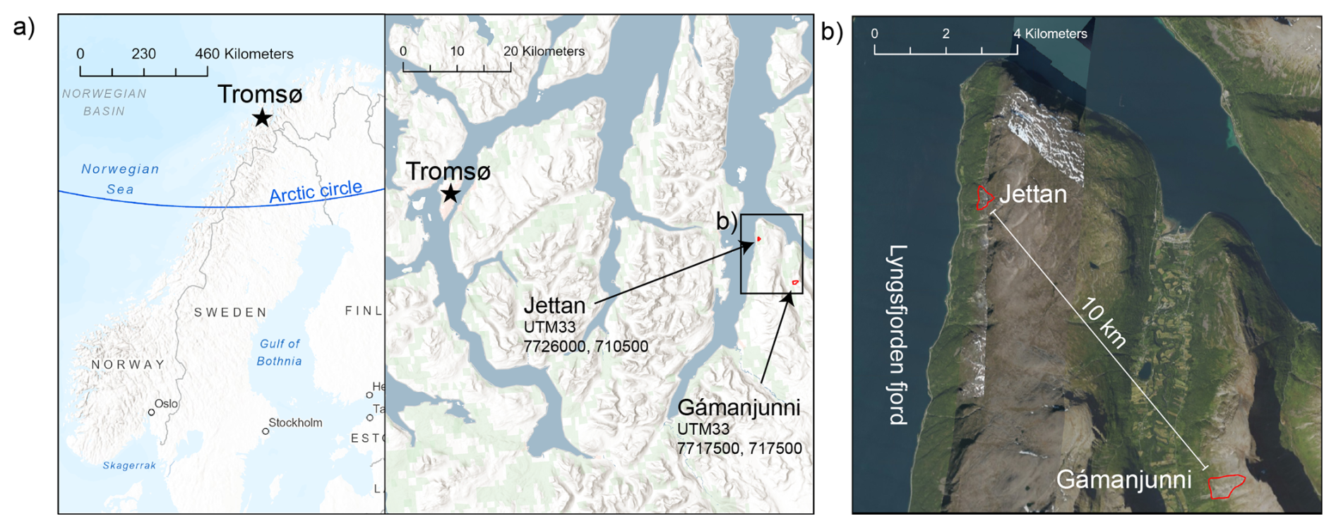
Figure 1 Location of the two landslides, Jettan and Gámanjunni, with their UTM33 GPS coordinates ($\mathrm{69}\mathit{°}{\mathrm{33}}^{\prime }{\mathrm{25.7}}^{\prime \prime }$ N, $\mathrm{20}\mathit{°}{\mathrm{24}}^{\prime }{\mathrm{38.5}}^{\prime \prime }$ E, and $\mathrm{69}\mathit{°}{\mathrm{28}}^{\prime }{\mathrm{50.8}}^{\prime \prime }$ N, $\mathrm{20}\mathit{°}{\mathrm{34}}^{\prime }{\mathrm{10.2}}^{\prime \prime }$ E, respectively). (a) Map of Scandinavia, the Arctic Circle, and the location of the landslides east of the city of Tromsø (Credit: Esri | Powered by Esri). (b) A zoom-in of the two landslides highlights their spatial distance of less than 10 km (© Kartverket. All rights reserved).

Table 1 Comparison between the two landslides.

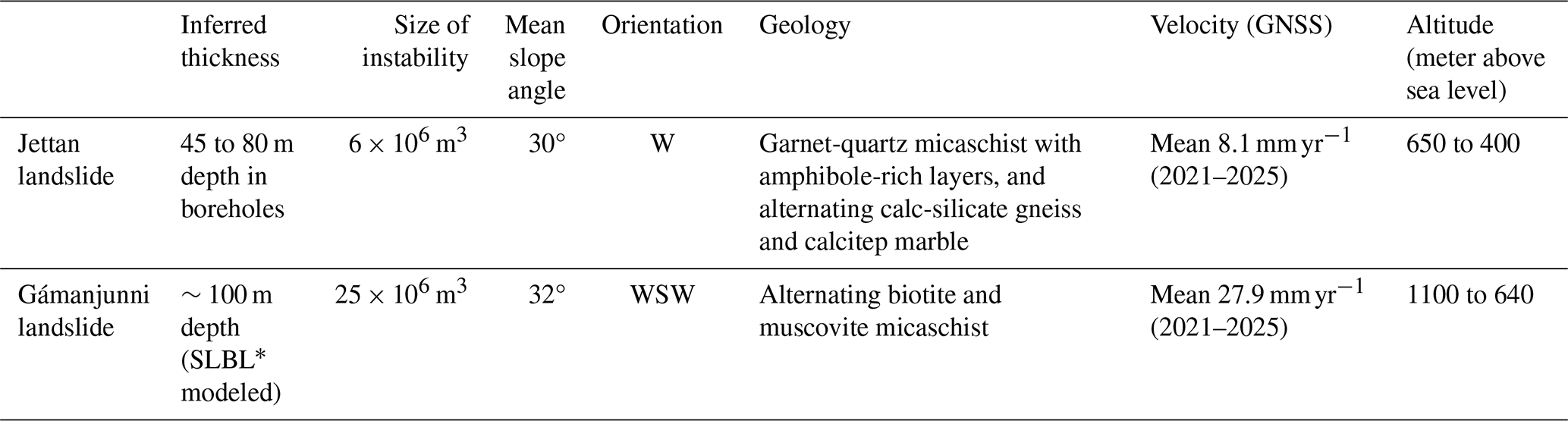
^∗ Sloping Local Base Level (SLBL) from Böhme et al. (2016a).

2.1.1 Jettan Landslide

The Jettan active landslide is situated along the Lyngsfjorden fjord and is one of several landslides on the Nordnesfjellet's west-facing slope (Fig. 2). It slides at an average velocity of up to 12 mm yr⁻¹ along an average slope of 30°, and includes cliffs of up to 40 m in height (Braathen et al., 2004). The landslide extends from approximately 200 to 900 m above sea level (m a.s.l.) and is bounded by two active back-scarp fractures. The volume of the active landslide is estimated to be six million cubic meters (Blikra et al., 2015). The annual theoretical probability of failure has been estimated to be between $\mathrm{1}/\mathrm{100}$ and $\mathrm{1}/\mathrm{1000}$ (NGU, 2025; NVE, 2024; Hermanns et al., 2013). If it fails abruptly, it could cause a devastating tsunami in the fjord below.

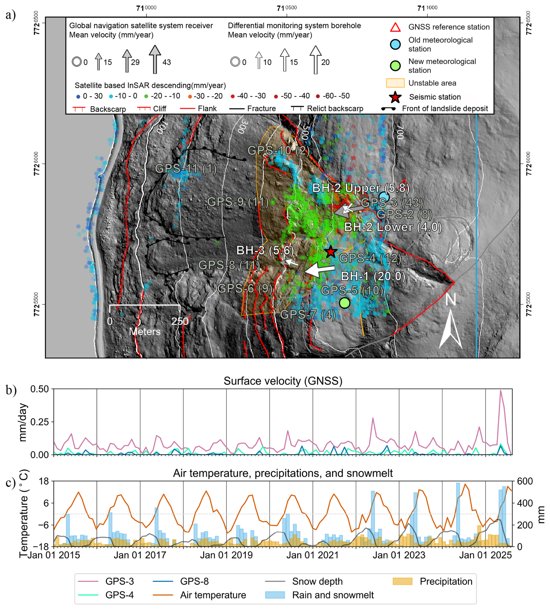
Figure 2 Overview of the Jettan landslide. (a) Map showing key morphological features and instrument locations (© Kartverket. All rights reserved.). Gray arrows represent mean surface velocities (mm yr⁻¹) derived from GNSS data, while white arrows indicate borehole shear zone displacements from the differential monitoring system (BH), both averaged over the period from 1 January 2021 to 12 August 2025. Arrow dimensions are scaled proportionally to velocity magnitude, with values annotated in parentheses. Borehole BH-2 displays two arrows corresponding to distinct shear zones. The blue solid line indicates the elevation above which permafrost is highly probable (Magnin et al., 2019). White contour lines denote 100 m elevation intervals. Hillshade based on Høydedata (© Kartverket. All rights reserved.). Time series plots display (b) GNSS velocity and (c) meteorological time series over the past decade. The GNSS velocity is calculated by a linear regression over one day and smoothed by down-sampling to 30 d median intervals, while the rainfall, snowmelt, and total precipitation is down-sampled to 30 d cumulative intervals.

The rocks consist of garnet-quartz-mica schists with amphibole-rich layers in the lower parts of the front of the landslide and layers of alternating calc-silicate gneiss and calcite marble in the uppermost part of the landslide of the Nordmannvik Nappe (Zwaan et al., 2006; Skrede, 2013). The nappe unit exhibits high strain and several internal thrust faults. The Jettan landslide is located within one of these faults (Andresen, 1988). The rocks display a distinct foliation dipping approximately 20° towards the west, and two dominant fracture sets are striking NE-SW and ESE-WNW (Braathen et al., 2004; Skrede, 2013; Vick et al., 2021). The back-scarp is approximately 750 m long, starting in the north with a 100 m high cliff segment, then gradually reducing to sinkhole lineaments in the middle, and further steep slopes on the south side. Several geological sub-units show evidence of ductile deformations, such as garnet-quartz-mica schist with blastomylonites and calc-silicate gneiss lenses that contain boudins of amphibole and calcite marble up to tens of meters long (Skrede, 2013). Electric resistivity and refraction seismic data suggest that the rocks are fractured to approximately 50 m depth and indicate possible sporadic permafrost (Rønning et al., 2008). Temperature measurements in three 100 m-deep boreholes within the landslide display positive temperatures ranging from 2 to 4 °C. In contrast, measurements from temperature sensors in the open back-fracture adjacent to borehole BH-1 indicate subzero rock-wall temperatures during parts of the year and the presence of multi-year ice at the fracture bottom (Blikra et al., 2015), despite the landslide being located below the modeled permafrost boundary (Magnin et al., 2019).

Drill core logs show narrow shear zones in the boreholes. In two out of three boreholes, clays have been detected in the shear zone (Ganerød, 2013, 2014). Analyses of optical televiewer data show that the entire borehole contains fractures. In all boreholes, fractures at the depth of the shear zone dip westward towards the fjord, with angles of approximately 15° in boreholes BH-1 and BH-3 and between 55 and 75° in BH-2 (Elvebakk, 2013, 2014).

2.1.2 Gámanjunni Landslide

The Gámanjunni landslide lies within the Manndalen valley, which contains several landslides and large rock avalanche deposits along its west-facing mountain slope (Fig. 3). It slides at an average velocity up to 40 mm yr⁻¹, on an average slope of 33°. The landslide consists of a large fractured block that extends from approximately 640 to 1100 m a.s.l. and is bounded by the back-scarp, which consists of two surfaces forming a wedge. The volume of the landslide is estimated to be 25×10⁶ m³ (Böhme et al., 2016b). The annual theoretical probability of failure is more than $\mathrm{1}/\mathrm{100}$ (Geological Survey of Norway (NGU), 2025; NVE, 2024; Hermanns et al., 2013). Upon sudden failure, the landslide could potentially dam the river below, which may cause a devastating flood if this dam were to fail.

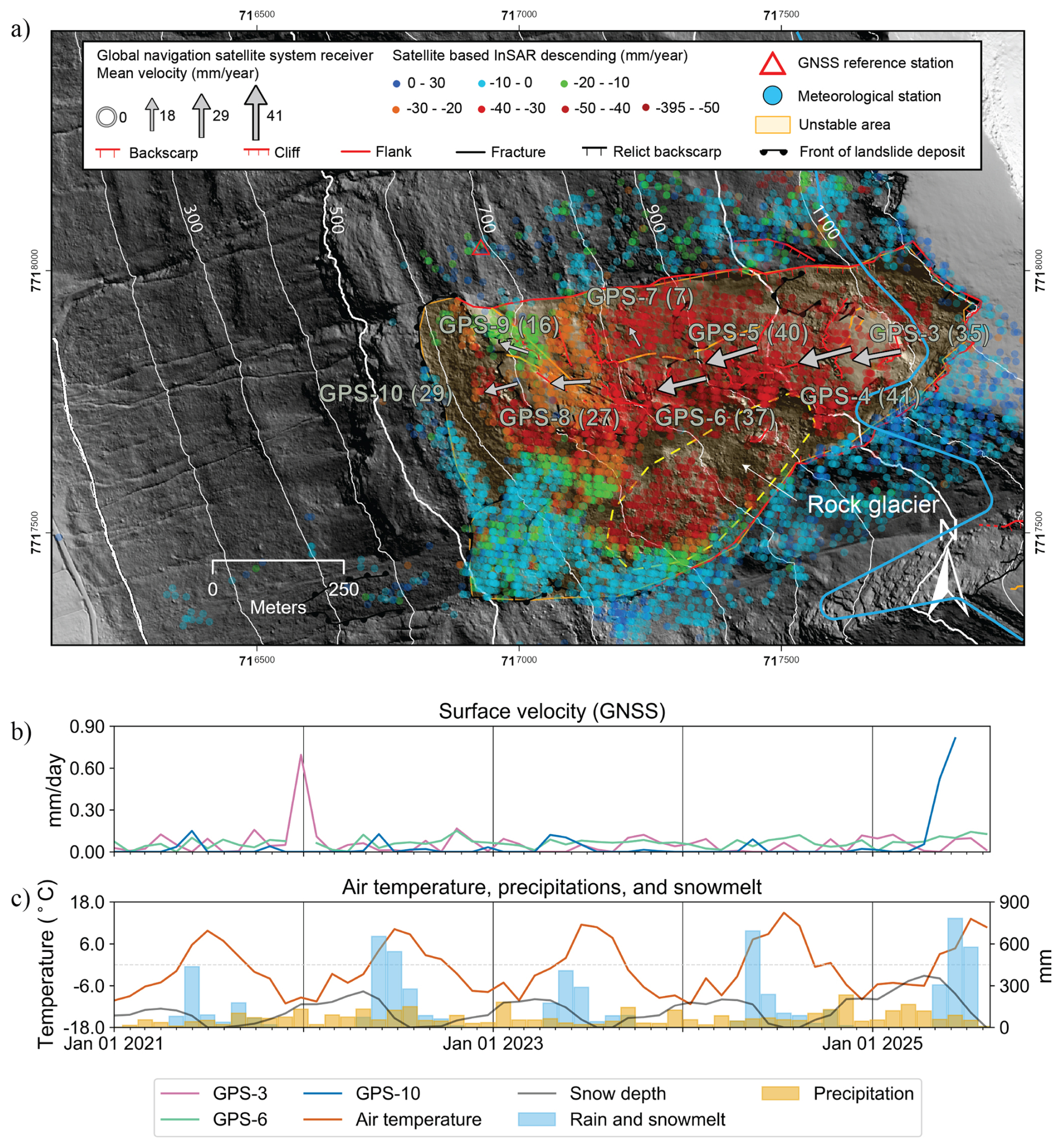
Figure 3 Overview of the Gámanjunni landslide. (a) Map illustrating key morphological features and instrument locations. Gray arrows denote mean GNSS-derived surface velocities (mm yr⁻¹) calculated for the period from 1 January 2021 to 12 August 2025, with arrow size scaled to velocity magnitude and annotated values in parentheses. The blue solid line indicates the elevation above which permafrost is highly probable (Etzelmüller et al., 2022). The yellow dashed outline delineates the active rock glacier extent. Elevation contours are shown in white at 100 m intervals Hillshade based on Høydedata (© Kartverket). Accompanying plots display (b) GNSS velocity and (c) meteorological time series over the past five years. The GNSS velocity is calculated by a linear regression over one day and smoothed by down-sampling to 30 d median intervals, while the rainfall, snowmelt, and total precipitation is down-sampled to 30 d cumulative intervals.

The rocks consist of micaschist from the Kåfjord Nappe, characterized by a higher proportion of biotite than muscovite, with amphibole-rich layers and lenses. One of the internal thrust faults from the nappe unit is located in the valley below the Gámanjunni landslide (Böhme et al., 2016b; Quenardel and Zwaan, 2008). There are two fracture sets in the area, striking WNW-ESE and NE-SW. The foliation is dipping on average 8° towards 312°. The back-scarp is dipping on average 51° towards 217° on one side and 58° towards 305° on the other side. The surfaces are very well developed and show progressive failure of rock bridges between the foliation layers (Böhme et al., 2016a). Electric resistivity data suggest an approximate thickness of 10 to 20 m of highly fractured rocks (Böhme et al., 2016a). The landslide lies above the modeled permafrost boundary (Magnin et al., 2019), and potential permafrost extent ranges from small areas near the top plateau (Böhme et al., 2016a), down to elevations of about 800 m a.s.l., and may include a subsurface layer thickness of 30–50 m within the landslide mass (Hauck and Hilbich, 2018; Etzelmüller et al., 2022).

2.2 Geophysical Monitoring and Processing

The Norwegian Water Resources and Energy Directorate (NVE) manages the early warning systems for the two landslides. The Jettan and Gámanjunni landslide monitoring systems have been improved over time with several instruments added over the years. The Jettan landslide dataset consists of a wide range of instruments that measure displacement, groundwater level, seismic activity, and meteorology (for additional information, see Table A1). The Gámanjunni landslide dataset is limited to surface displacement and meteorological data, with no borehole or seismic measurements available to constrain subsurface conditions (for additional information, see Table A2). Borehole installations at the Jettan landslide site proved technically challenging, while at the Gámanjunni site, drilling was not undertaken due to prohibitive costs.

2.2.1 Surface Displacement Data

The Global Navigation Satellite System (GNSS) sensors are spatially distributed on the two slopes, with ten and eight instruments for the Jettan and Gámanjunni landslides, respectively. For both landslide sites, relative positioning is employed using a reference GNSS receiver located on stable ground, within 0.5 km of each landslide. The data are post-processed in 12 h intervals to derive surface displacements with millimeter-level precision (σ=0.6 mm), as estimated by Cautus Geo, the company that supplied the Trimble equipment and performed the time series processing. To reduce the noise associated with height measurements, we utilized the northing and easting components to construct two-dimensional displacement vectors. At the Gámanjunni landslide site, the initial reference receiver was not installed on stable ground, which rendered the data unreliable, while the subsequent reference station was affected by ice accumulation that degraded the signal from 28 December 2021 to 7 February 2022. Consequently, only data acquired with the new reference station, after removing the period during which the antenna was iced, are included for the analysis.

2.2.2 Borehole Displacement and Hydrologic Measurements at the Jettan Landslide

Four boreholes were cored and logged, three of which are currently instrumented with a Differential Monitoring System (DMS) supplied by the company Centro Servizi di Geoingegneria (CSG s.r.l). These instruments are calibrated and tested before installation (Foglino et al., 2015). The boreholes BH-1, BH-2, and BH-3 are named according to the order of instrumentation, with BH-1 drilled and instrumented first (Table A3). The DMS 2D Rock system was installed in a plastic borehole casing containing strings of one-meter bi-axial inclinometers extending to a depth of approximately 100 m. A piezometer was placed near the bottom in each borehole, and all sensors record measurements at hourly intervals (Fig. 4). The movement of the landslide gradually induces deformation of the boreholes, which will ultimately lead to instrument failure. While deforming, we obtain displacement in millimeters in the north-south and east-west directions. Data are downloaded from the software DMS EW (CSG, 2007). We analyze the entire time series of the boreholes, i.e., 11-year-long (BH-2 and BH-3) and 12-year-long (BH-1) series.

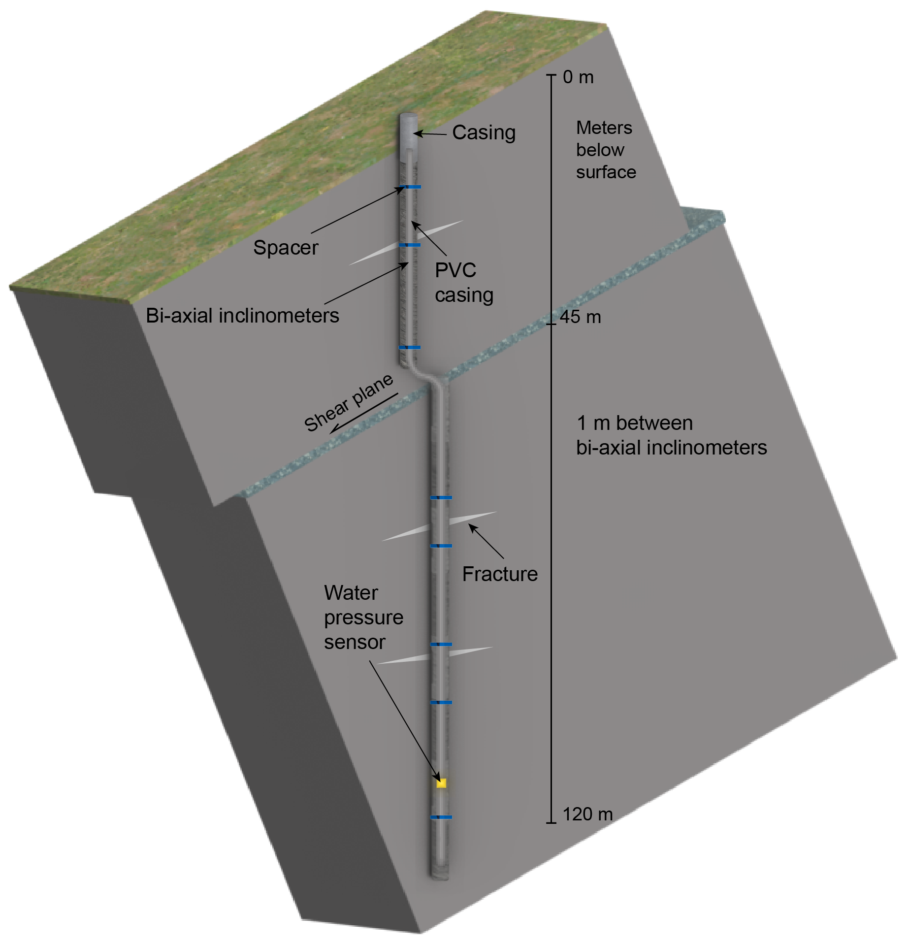
Figure 4 Conceptual sketch (not to scale) of the BH-1 borehole instrumentation. The borehole intersects the landslide shear surface and extends into the underlying bedrock. The installation consists of a chain of 120 bi-axial inclinometers housed within a PVC casing and a water pressure sensor located four meters above the base of the open borehole for hydraulic head measurements. The instrumentation enables simultaneous monitoring of subsurface displacement and groundwater pressure within the landslide.

2.2.3 Surface Broadband Seismic Station Data at the Jettan Landslide

Monitoring apparent surface wave velocity provides insights into the variations of the mechanical characteristics of the subsurface. Velocity variations are caused by changes in rigidity (the shear modulus), density, pore water pressure and temperature (Le Breton et al., 2021). In the case of mountain and arctic regions, temperature has also been proposed to be a driving mechanism of seismic velocity variation through icing/de-icing effects at surface and permafrost decrease (Albaric et al., 2021).

The variation of apparent surface wave velocity ($\mathrm{d}v/v$) inside the landslide between 2016 and 2025 was computed using single-station correlation of ambient seismic noise (Hobiger et al., 2014) at station JETT, which is operated by the Norwegian Seismic Array (NORSAR, 1971). A complete description of the processing is provided in Appendix (Sect. A1). The station is a 3-component CMG broadband velocimeter operating at a frequency of 200 Hz. For each of the three possible pairs of components (Vertical-North, Vertical-East, and North-East), data were cut into 1 h-long time series. They were standardized, filtered between 1 and 50 Hz, and then whitened in the same frequency range to set its spectral amplitude to 1. The data were cross-correlated, and the daily correlogram was computed as the average of the 24 hourly correlograms. Velocity variations were computed using the stretching technique (Sens-Schönfelder and Wegler, 2008; Hadziioannou et al., 2009). First, the three matrices of daily correlograms were denoised using a singular value decomposition Wiener filter (Moreau et al., 2017), with a filter size of 7 in both dimensions (days and lag), and a number of singular values of 20. A reference correlogram was computed (the average of the 2543 available daily correlograms), and each daily correlogram was stretched and compared to the reference. Stretching was conducted in the lag range of $[-\mathrm{2}:-\mathrm{0.2}]$ and [0.2:2] s and in the frequency range 3–8 Hz (see Sect. 2.2.5). This lag range corresponds to the near coda, away from ballistic waves, and is therefore less sensitive to source variability. Eventually, $\mathrm{d}v/v$ was computed as the average of the three $\mathrm{d}v/v$ time series, weighed by their coefficient of correlation (Hobiger et al., 2014). The coefficient of correlation quantifies the similarity between the reconstructed waveforms, where a low coefficient (strong decorrelation) is associated with structural changes and also fluid injection into the subsurface (Larose et al., 2015; Le Breton et al., 2021).

2.2.4 Meteorological Data

The meteorological station at the Jettan landslide was installed in 2014 above the back scarp (blue circle in Fig. 2). Due to its location on an inclined slope next to other buildings, which influenced the measurements, a new meteorological station was installed further south above the back scarp in 2022 (green circle in Fig. 2). For the Gámanjunni landslide, the meteorological station was installed on the plateau above the landslide in 2017 (blue circle in Fig. 3). For comparing the Jettan and Gámanjunni landslides, we utilized seNorge data (seNorge, 2024) for all meteorological parameters at both sites. This approach was chosen because the meteorological station at Gámanjunni is located approximately 200 m above the landslide, and because continuous snow measurements are not available at Jettan. The modeled variables were therefore extracted at the elevation of each landslide (557 and 820 m a.s.l. for Jettan and Gámanjunni, respectively), allowing elevation-consistent comparison while providing snow variables unavailable from in situ observations. seNorge is a weather model service provided by the Norwegian Water Resources and Energy Directorate, Norwegian Meteorological Institute, the Norwegian Public Road Administration, and the Norwegian Mapping Authority. The model utilizes all approved meteorological stations in Norway, including the landslide stations, to provide 1 km grid cells of daily interpolated meteorological data that are locally weighted (seNorge, 2024; Lussana, 2021). The relocation of the Jettan weather station improves snow accumulation measurements, which could bias the long-term trends of modeled meteorological variables. In addition to surface temperature, precipitation, snow depth, and snowmelt and rain from the seNorge model, we have modeled ground temperatures at 1, 45, and 115 m depth by using the CryoGrid community model (Westermann et al., 2023). Details of the model setup are provided in the Appendix (Sect. A2).

2.2.5 Integration of Data

We utilized ArcGIS software (ESRI, 2023) to visualize the displacement data spatially. The 1 m digital elevation models were downloaded from Høydedata (Høydedata, 2024) for both landslides and were used to plot altitude contours and create topography profiles, enabling evaluation of failure scenarios.

To delineate periods of expected ground freezing and thawing, we derived a freeze index, which is the monthly ratio of days with mean air temperatures above 0 °C to those below 0 °C. Freeze index values above one indicate more days above 0 °C, while values below one indicate more days below 0 °C.

To calculate the total displacement in the borehole, it is necessary to sum the displacements recorded by all the inclinometers (Aspaas et al., 2024; Ruggeri et al., 2020). We obtained the maximum displacement in the slip direction for each inclinometer by calculating the maximum amplitude and its orientation. We extracted displacement components in the north and east directions, calculated the magnitude and mathematical azimuth, and then converted the azimuth to compass bearings. Then, we plotted the cumulative displacement of the borehole and identified zones of increased displacement, i.e., the shear zones (Fig. 5). A few electrical or technical errors on the borehole instruments have been resolved by remote resets of the modules, resulting in the displacement being reset to zero. We have resolved these incidents by raising the displacement to the previous level, with a one-day median difference before and after the reset. In addition, we removed a few abrupt, significant spikes in the time series due to lightning strikes. We filtered the GNSS and borehole time series using a coarse outlier removal of three standard deviations, followed by a linear interpolation to fill data gaps and a Savitzky-Golay filter (SciPy Developers, 2025) in combination with a 14 d centered rolling median filter (Pandas Developers, 2025b). To estimate the sliding velocity, we calculate the slope of a centered rolling linear regression of the filtered displacement time series. For each time step t, we consider a symmetric window of W days centered on t, and fit a straight line to the displacement values within the window. For all plots presented in this manuscript, a window length of W=1 d was used. The slope of this line v(t) represents the velocity at time t:

$$\begin{array}{}\text{(1)}& v\left(t\right)={\displaystyle \frac{{\sum }_{i=\mathrm{1}}^W(x_i-\stackrel{\mathrm{‾}}{x})(y_i-\stackrel{\mathrm{‾}}{y})}{{\sum }_{i=\mathrm{1}}^W(x_i-\stackrel{\mathrm{‾}}{x}{)}^{\mathrm{2}}}},\end{array}$$

where we compute the local linear regression of displacement y_i against time x_i.

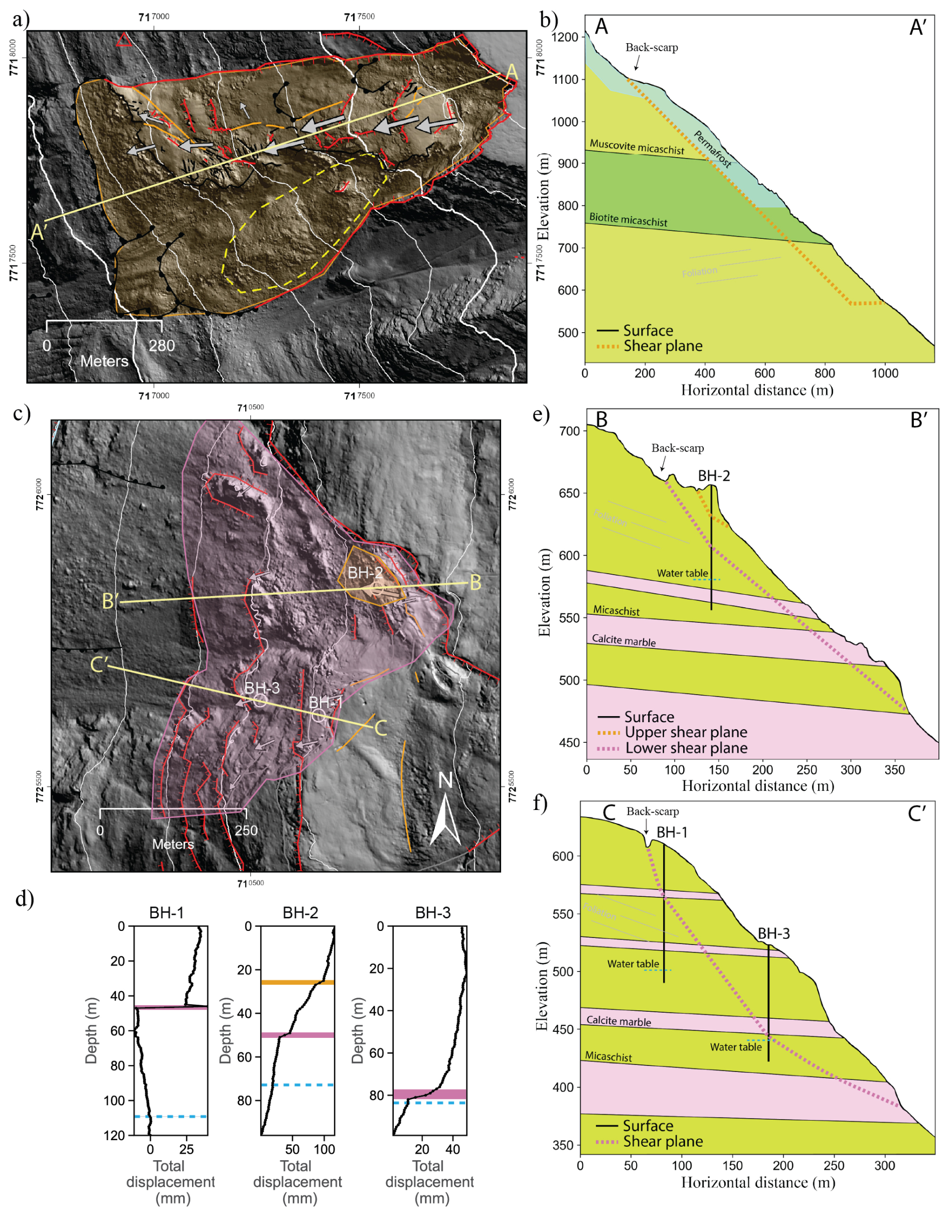
Figure 5 Schematic representation of the Gámanjunni and Jettan landslides. (a) Map of Gámanjunni with profile A-A^′. (c) Map of Jettan with profiles B-B^′ and C-C^′, and associated associated boreholes (BH-1 to BH-3). (b, e, f) Geologic cross-sections showing lithology, foliation, interpreted shear zones, permafrost extent, boreholes, and hydraulic head. (d) Borehole displacement data indicating one or two shear zones. Displacements are shown in the slip direction and represents maximum recorded values. Axis scales differ among plots. Orange and pink lines denote the interpreted upper and lower shear zone, respectively, while the dashed blue line indicates the maximum hydreulic head. Shear zones were inferred from borehole observations and mapped morphological features. Semi-transparent orange and pink polygons indicate the proposed sliding scenarios.

Temporal aggregation of the time series was performed by resampling the data to coarser temporal resolutions using the resample method (Pandas Developers, 2025a). Within each resampling interval, values were aggregated using either the sum or the median, depending on the data type: precipitation variables (rain and snow) were summed, while temperature and displacement data were aggregated using the median. This procedure resulted in regularized time series at daily, weekly, or monthly resolution, depending on the requirements of the specific analysis. A centered rolling window was applied to compute running sums of meteorological variables (Pandas Developers, 2025b). Centering the rolling window minimizes time-lag effects across different window lengths, as illustrated in Fig. A1.

Creep bursts were identified from the borehole displacement time series using the short-term-average and long-term-average difference (STA-LTA) algorithm from Aspaas et al. (2024). Short-term and long-term velocities were computed using moving windows of 32 and 120 d, respectively. A creep burst was recorded when the STA–LTA difference exceeded a threshold of 1.5 standard deviations.

To analyze structural changes within the landslide, we evaluated the sensitivity of seismic surface waves with depth and frequency to obtain the correct frequency range, scanning the entire unstable mass. To achieve this, a vertical velocity model was defined using data available for the site (Blikra and Christiansen, 2014; Vick et al., 2021; Rønning et al., 2008), and empirical relationships (Brocher, 2005) to evaluate P- and S-wave velocities for missing data. The sensitivity kernels for both Rayleigh and Love waves were computed using the Disba package (Luu, 2021). Results show that the frequency range of 3–8 Hz is suitable for monitoring the active landslide at depths of approximately 10 and 50 m. Details of the seismic velocity model are provided in the Appendix (Sect. A2).

To quantify relationships among variables, we first aligned the temporal resolution of the datasets and applied time series filtering without introducing time shifts between series. The data were then scaled using the MinMaxScaler function from the Python package sklearn (scikit-learn developers, 2024) to obtain similar weights across variables. We assessed stationarity using the Dickey-Fuller test (Perktold et al., 2023). Cross-correlation was performed using Spearman rank correlation as it is non-parametric and suitable for time series data, which often violate normality assumptions. Lags analysis was limited to three months to capture seasonal effects, as longer-term correlations across seasons are unlikely to represent causal relationships.

To further develop quantitative relationships between different variables and their explanatory power for the resulting movement in the boreholes, we employed a dynamic regression model, specifically the AutoRegressive Distributed Lags (ARDL) model. This modeling approach allows explaining a time series (i.e., the sliding velocity, called the endogenous variable) using the time series of other variables (i.e., water pressure, rain, or snowmelt, called the exogenous variables). The autoregressive (AR) component of the model accounts for the influence of the endogenous variable's own past values, meaning that yesterday's sliding velocity influences today's sliding velocity. The distributed lag (DL) component captures the delayed effects of the exogenous variables on the endogenous variable, meaning that yesterday's water pressure influences today's sliding velocity. In the ARDL model, each variable can have its own lag order. For example, in a model with sliding velocity and water pressure, sliding velocity may include three lags and water pressure two lags, resulting in a lag structure of (3, 2). Assuming daily data, this means that today's sliding velocity depends on its previous three days and the previous two days of water pressure (Bismans, 2025).

Due to the large size of the dataset, the original ardl_select_order function from the Statsmodels ARDL package (Perktold et al., 2023) was computationally inefficient for determining the optimal lag structure. By optimal lag structure, we mean the best combination of lag lengths for both endogenous and exogenous variables that provides the best model fit. To address this limitation, we revised the function to improve efficiency and enable robust lag selection for endogenous and exogenous variables according to the Bayesian Information Criterion (BIC). BIC discourages overfitting by penalizing model complexity, and lower values indicate better model fit. The lag search was restricted to a maximum of three months under the assumption that all exogenous variables would influence the endogenous variable within that time frame. Since this process is computationally intensive, we down-sampled the time series to weekly intervals. Displacement, groundwater pressure, air temperature, ground temperature, and temporal variation in seismic velocity were mean-averaged, while precipitations were summed. A sensitivity analysis comparing a 2.5-year subset of the daily data with its weekly equivalent demonstrated negligible differences in the inferred relationships, indicating that weekly sampling adequately captured the observed dynamics.

Once the optimal lag structure was identified, the ARDL model was fitted using the following ARDL function (Perktold et al., 2023):

$$\begin{array}{}\text{(2)}& Y_t=\sum _{p=\mathrm{1}}^P{\mathit{\alpha }}_p{Y}_{t-p}+\sum _{k=\mathrm{1}}^M\sum _{j=\mathrm{0}}^{Q_k}{\mathit{\beta }}_{k,j}{X}_{k,t-j}+{\mathit{ϵ}}_t,\end{array}$$

where Y_t represents the endogenous variable at time t. The first summation represents the autoregressive component, where past values of Y up to lag P are included, where α_p is the estimated coefficient. The second summation corresponds to the distributed lag component, which accounts for the influence of M exogenous variables. For each exogenous variable X_k, both its current value and lagged values up to Q_k are included, with associated estimated β coefficients for variable k at lag j. The estimated α and β coefficients indicate the magnitude of the variable's effect on the endogenous variable, where a larger absolute value indicates a stronger influence. The term ϵ_t represents the error in the model.

To evaluate the model's predictive performance, we split the selected time series into training and test datasets using a ratio 80:20. To isolate the contribution of the autoregressive dynamics, we also fitted a simplified Distributed Lag (DL) model by setting the lagged endogenous terms to zero. In this configuration, the DL model predicts the endogenous variable solely from current and lagged values of exogenous variables.

This comparison enables an assessment of whether including AR terms improves model performance. We evaluated both models using the BIC score, following the interpretation thresholds in Table 6 of Raftery (1995), and compared their root-mean-squared errors (RMSE) of the out-of-sample test data.

3 Results

3.1 Jettan and Gámanjunni Surface Velocities

At the Jettan landslide, we study the period from 1 January 2015 to 12 August 2025, where the mean rate of horizontal displacement across all GNSS receivers (except GPS-3) is 8 mm yr⁻¹, varying from 6 mm yr⁻¹ in 2015–2016 to 11 mm yr⁻¹ in 2025. The displacement time series shows a distinct seasonal trend for all GNSS receivers, which is most pronounced at GPS-3 (Fig. 2). GPS-3 is situated on a kinematically distinct block that is structurally separated from the main landslide body. As this block moves independently from the main landslide, we excluded it to calculate the mean displacement rate of the landslide. The location of this block is highlighted in Fig. 5.

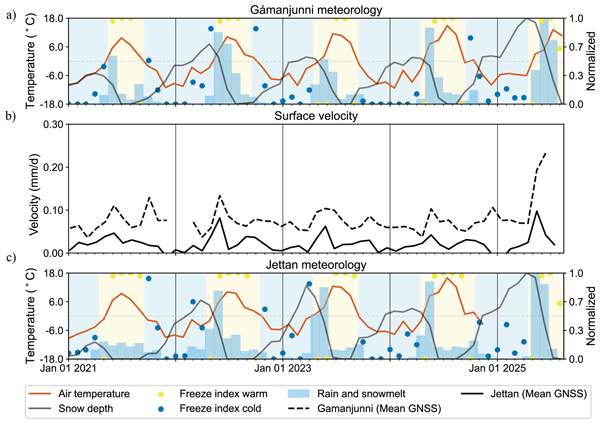
At the Gámanjunni landslide, we study the period from 1 January 2021 to 12 August 2025, where the mean horizontal displacement rate for all GNSS receivers is 28 mm yr⁻¹, fluctuating from 24 mm yr⁻¹ in 2022–2023 to 39 mm yr⁻¹ in 2025. There is a distinct seasonal component in the displacement data, most noticeable at GPS-10 where the frontal lobe of the landslide accelerates in late spring. The seasonality is less pronounced for the other GNSS receivers relative to the Jettan landslide (Fig. 3). The mean displacement rate since 2021 is more than three times that of the Jettan landslide. Both Jettan and Gámanjunni display clear seasonal fluctuations in the GNSS data, with peak velocities in late spring and late autumn. For both landslides, we report mean horizontal displacement rates calculated across all GNSS receivers, excluding GPS-3 at Jettan (Fig. 6).

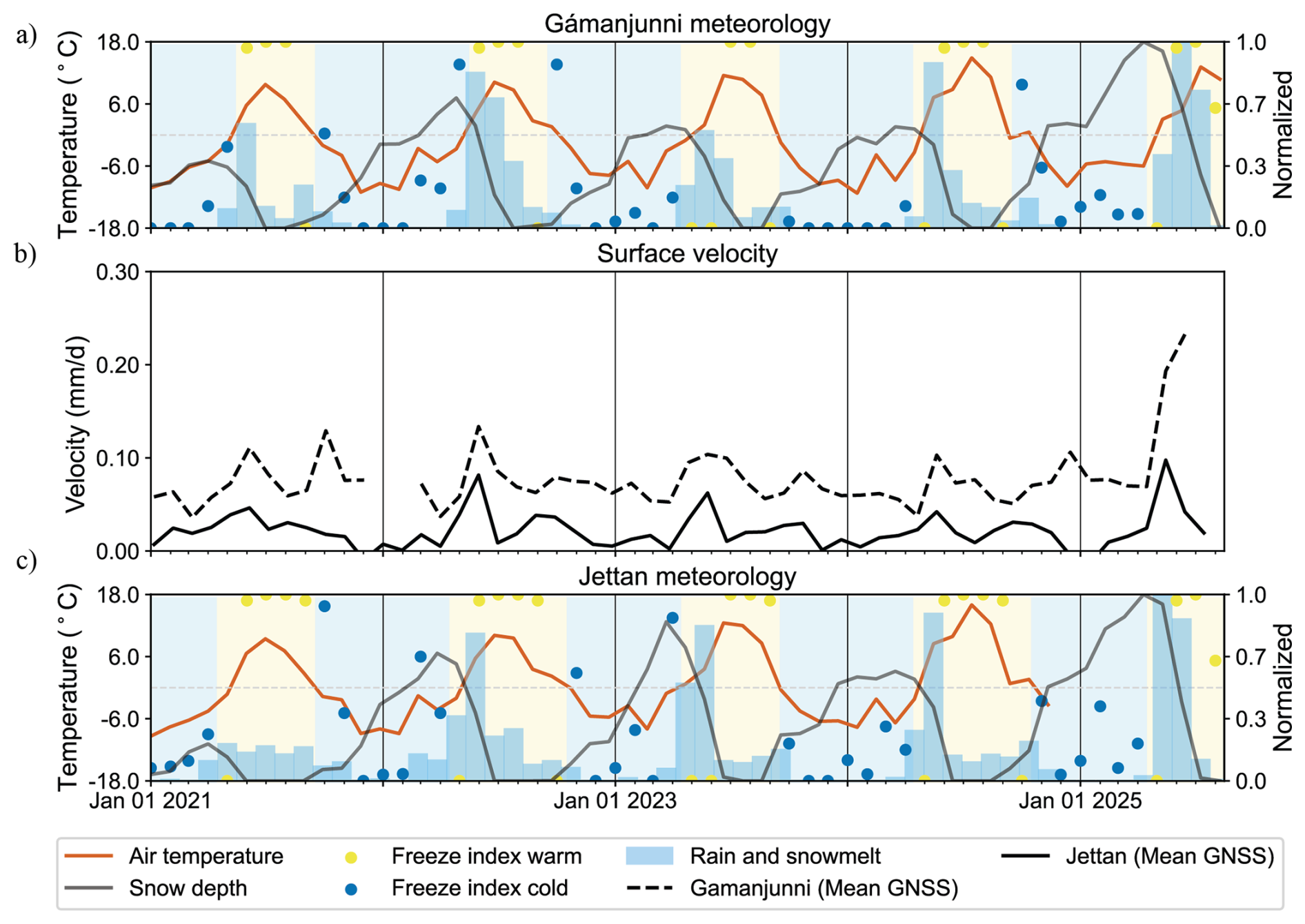
Figure 6 Time series of the air temperature and normalized freeze index, precipitation, and rain and snowmelt are displayed in (a) and (c) for the Gámanjunni and Jettan landslides, respectively. The transparent blue and yellow background highlights cold and warm periods based on the freeze index, facilitating comparison of these periods between the two landslides. The time series of the mean velocity of all GNSS receivers for the Jettan and Gámanjunni landslides (except GPS-3 for Jettan) are shown in (b). All time series have been smoothed by down-sampling to a 30 d median or summation for precipitation and rain and snowmelt.

3.2 Borehole Data at the Jettan Landslide

At the Jettan landslide, we compare the cumulative displacement over all inclinometers in the boreholes and the nearest GNSS receivers over the period from 1 January 2020 to 1 January 2024. Borehole BH-1 displays a cumulative displacement of 36 mm, while GPS-4 and GPS-5 display 46 and 40 mm, respectively. Borehole BH-2 displays a cumulative displacement of 163 mm, while GPS-3 displays 157 mm, and borehole BH-3 displays a displacement of 59 mm, while GPS-8 displays 46 mm (Fig. 2). We can detect the shear planes from the cumulative displacement plots in Fig. 5. Analysis of the shear planes shows that borehole BH-1 is predominantly concentrated within the localized shear zone, whereas in BH-2 and BH-3, deformation is more broadly distributed and only weakly localized within the sliding zone. When we compare the displacement in sliding zones, we observe that boreholes BH-1 and BH-3 move at a similar rate (5 mm yr⁻¹) over the period from 2018 to 2020. Borehole BH-2 upper and lower shear zones have a slightly lower displacement rate (3 and 5 mm yr⁻¹). In 2020, borehole BH-1 started accelerating (7 mm yr⁻¹) and accelerated again in 2022 (21 mm yr⁻¹). During the first acceleration, borehole BH-3 also accelerated (6 mm yr⁻¹), but slowed down in 2022 (6 mm yr⁻¹). At the same time as the last acceleration of borehole BH-1, the amplitudes of the seasonality of borehole BH-2's upper shear plane almost doubled (from 3 mm yr⁻¹ in 2019 to 6 mm yr⁻¹ in 2022), and nearly tripled in 2025 (9 mm yr⁻¹). During this period, GPS-4 and GPS-8, located at boreholes BH-1 and BH-3, continued to move at a steady displacement rate (11 ± 1 mm yr⁻¹ from 2018 to 2024). Similarly, the lower shear zone of BH-2 maintained a displacement rate consistent with that of the upper shear zone, but without the seasonal fluctuations (4 ± 1 mm yr⁻¹ from 2018 to 2024).

The seasonal trends visible in the GNSS time series of Jettan are harder to spot in the borehole data. A clear seasonal pattern of increased velocity in late spring is pronounced for the upper shear zone in borehole BH-2, and infrequent bursts of slip acceleration occur in boreholes BH-1, BH-2 lower shear zone, and BH-3 (Fig. 7).

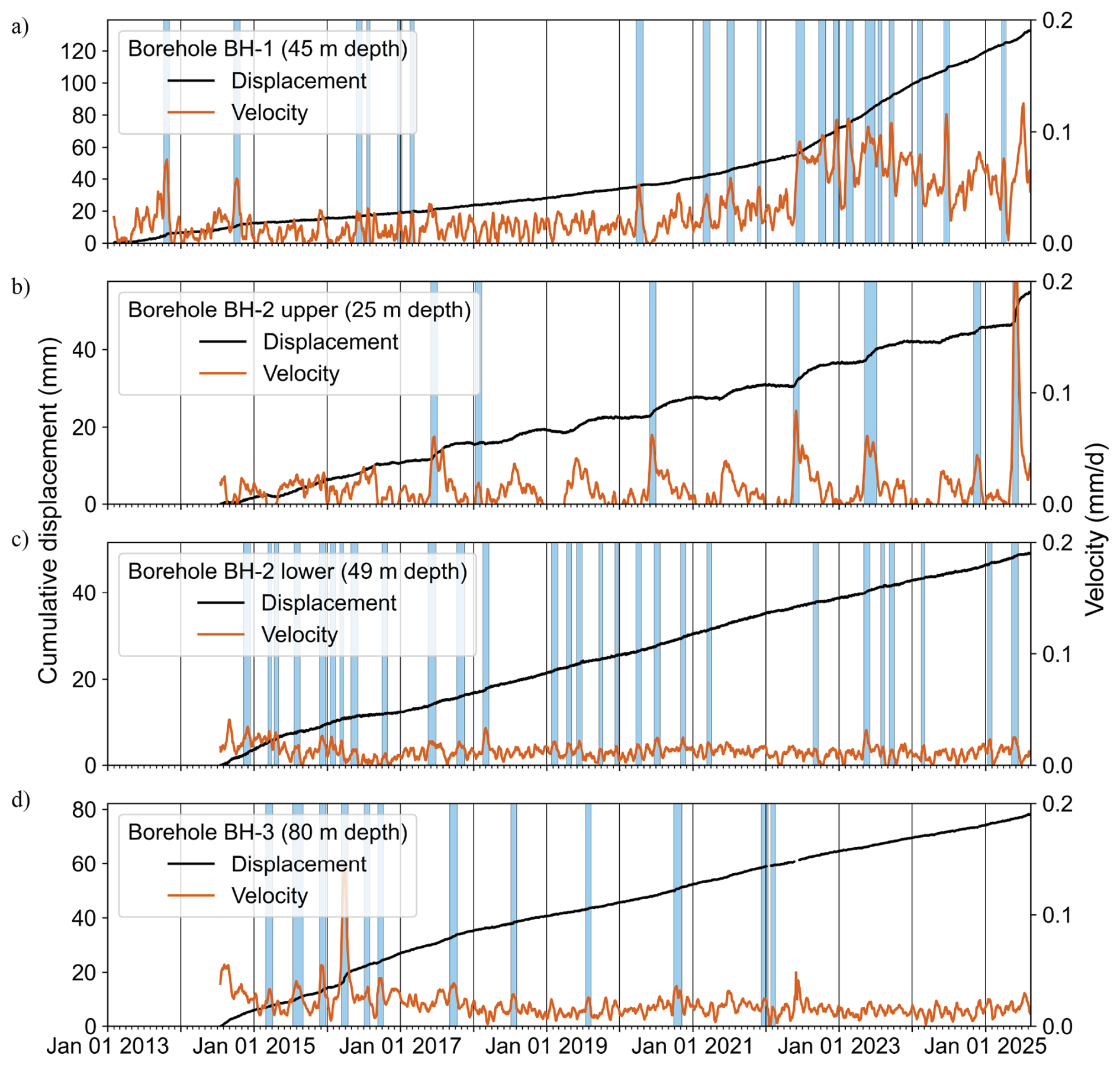
Figure 7 Time series of cumulative displacement (black) and velocity (orange) in the Jettan landslide. Data are measured in the shear zone inclinometers of borehole BH-1 (a), the two shear zones of borehole BH-2 (b, c), and the shear zone of borehole BH-3 (d) are presented. Shaded blue rectangular boxes indicate periods of detected creep bursts by the STA-LTA algorithm.

3.3 Seasonal Variations in Climatic Parameters and Seismic Velocity

Over the ten years from 1 January 2015 to 12 August 2025 at the Jettan landslide and the four years from 1 January 2021 to 12 August 2025 at the Gámanjunni landslide, the daily average median air temperature was 0.2 °C at Jettan, with a maximum of 23.9 °C in 2018 and a minimum of −18.9 °C in 2016, and −1.8 °C at Gámanjunni, with a maximum of 19.6 °C in 2022 and minimum of −19.0 °C in 2024. Modeled ground temperatures at borehole BH-1 (see Sect. 2.2.4, Appendix, Sect. A2) provided long-term trends beyond the borehole measurement period. The simulated mean annual ground temperature (MAGT) at 1 m depth over the last decade (2015–2025) was 2.4 °C, reflecting the thermal offset relative to air temperature. The model shows positive MAGT at both 45 and 115 m depths, indicating that no permafrost is present within the landslide body, which is consistent with recent borehole observations. Over the last 50 years, the simulated MAGT at 1 m depth increased by 0.2 °C per decade.

The freeze index for the two landslides shows shorter warm periods compared to cold periods for the Gámanjunni landslide on average, with a median of 0.51 ranging from 0.11 (2023) to 0.61 (2025), while the Jettan landslide has similar durations of warm and cold periods on average with a median of 1.24 ranging from 0.57 (2023) to 1.43 (2024) over the period from 1 January 2021 to 12 August 2025 (Fig. 6).

The median yearly rain and snowmelt is 940 mm, ranging from 659 mm in 2021 to 1254 mm in 2022 for the Jettan landslide area, and 1324 mm, ranging from 905 mm in 2021 to 1700 mm in 2022 for the Gámanjunni area. At the Jettan landslide site, water pressure recorded in borehole BH-1 consistently indicates minimal or absent pore pressure. In contrast, borehole BH-2 exhibits pronounced seasonal variations of up to 17 m, with peak levels occurring in spring and remaining elevated throughout the year. Borehole BH-3 shows a similar timing of the peak, but with a smaller amplitude of up to 5 m, followed by a sharp decline in water level (Fig. 8) The relative seismic velocity variation ($\mathrm{d}v/v$) exhibits a recurring seasonal pattern. It drops every spring and reaches two distinct minima below the two standard deviation threshold, one in summer and another in autumn. The signal then gradually recovers to near-baseline levels in mid-winter before the cycle begins again in spring (Fig. 9). For the period from 1 January 2016 until 31 July 2025, the $\mathrm{d}v/v$ trend is decreasing by −0.23 % yr⁻¹ (Fig. A3).

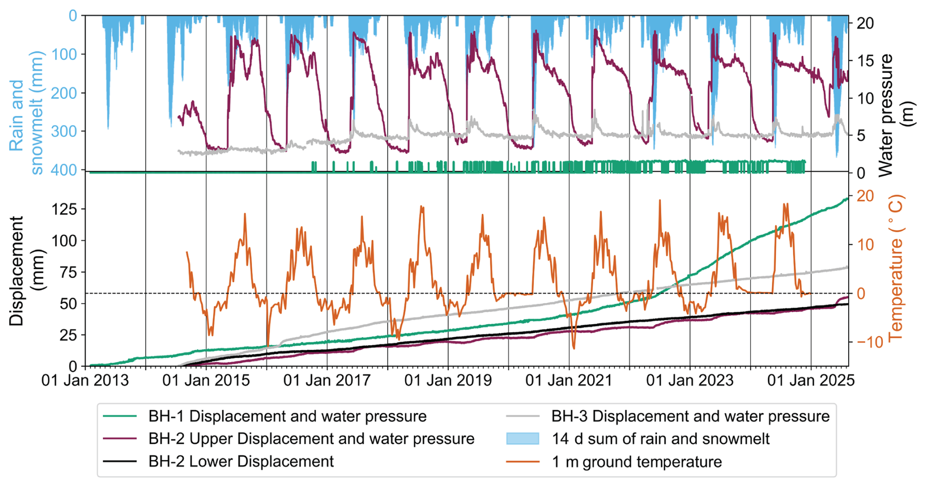
Figure 8 Time series of displacement in the shear zone and water pressure measured in boreholes BH-1 (mint green), BH-2 upper shear zone (purple) and lower shear zone (black), and BH-3 (orange), together with 14 d cumulative rainfall, snowmelt, and one meter depth ground surface temperature at the Jettan landslide.

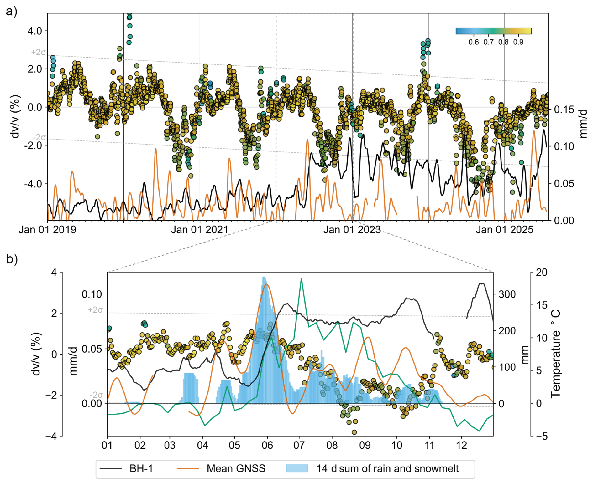
Figure 9 (a) The apparent surface velocity variations ($\mathrm{d}v/v$) with annual amplitude and long-term trend in the Jettan landslide, colored by cross-correlation values, and slip velocity recorded in borehole BH-1 (black curve) and mean GNSS velocity (orange curve). The stippled gray lines represent ± two standard deviations of $\mathrm{d}v/v$ around the linear trend over the full period. A seasonal drop below this threshold has been evident since 2020. (b) Detailed view of 2022 showing correlations between $\mathrm{d}v/v$ and seasonal accelerations in borehole BH-1, mean GNSS velocity, the 14 d running sum of rainfall and snowmelt, and modeled weekly ground temperature at 1 m depth.

3.4 Controlling Parameters of Landslide Velocity

3.4.1 Surface Displacement of the Jettan and Gámanjunni Landslides

Analyzing the time series from 1 January 2021 to 12 August 2025, based on 30 d mean velocity of all GNSS receivers (excluding GPS-3 at Jettan), reveals a moderate correlation between the two landslides with the spring acceleration at Jettan preceding that of Gámanjunni by 17 d (Pearson's r=0.49). The main differences between the two landslides are highlighted in Table 1. Focusing on the year 2022, the GNSS velocity at Jettan precedes that of Gámanjunni by 20 d (Pearson's r=0.54). At Gámanjunni, GNSS velocity exhibits a lag of approximately 20 d after peak rain and snowmelt when using a 14 d running sum, with a moderate to strong correlation (Pearson's r=0.52) during spring. At Jettan, the lag is about two days, with a strong correlation (Pearson's r=0.71). From September to December, after snowmelt has ceased, we observe no lag with a strong correlation between rain events and velocity increases for the Jettan landslide (Pearson's r=0.69). No comparable relationship is evident for the Gámanjunni landslide during this period.

3.4.2 Correlation of Borehole Accelerations with Groundwater Pressure, Climatic Parameters, and Changes in Seismic Velocities

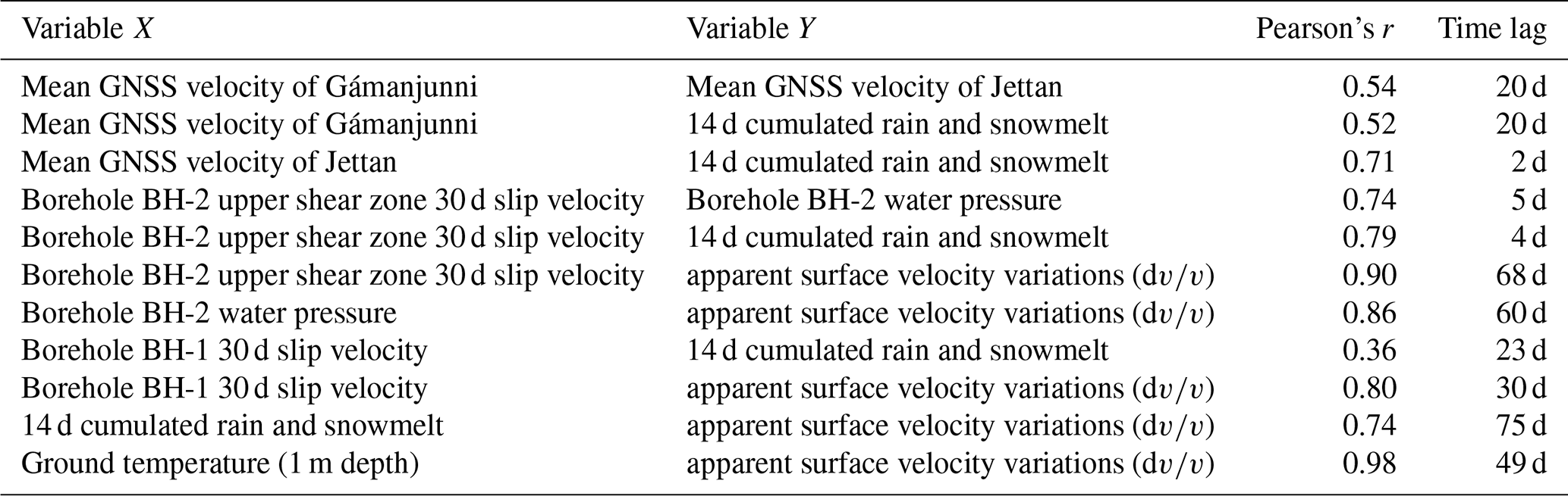
Borehole slip acceleration, hydrological variables, and seismic velocity changes in 2022 exhibit strong to very strong correlations, with systematic lags between forcing and response (Table 2). The 30 d slip velocity of the spring accelerations in the upper shear zone of borehole BH-2 and the changes in its water table display a strong correlation (Pearson's r=0.74) with a 5 d lag for the year 2022. The 2022 acceleration in borehole BH-1 and the upper shear zone in borehole BH-2 shows a moderate to very strong correlation between the 30 d velocity and the 14 d running sum of rain and snowmelt (Pearson's r=0.36 and 0.79), where the borehole velocity lags are 23 and 4 d, respectively. There is a very strong negative correlation with the drop in $\mathrm{d}v/v$ and the slip acceleration in borehole BH-1 and BH-2 upper shear zone (Pearson's coefficients $r=-\mathrm{0.80}$ and −0.90), where the $\mathrm{d}v/v$ lags are 30 and 68 d for the year of 2022. The rain and snowmelt, as well as ground temperature (1 m depth), also display a strong and very strong negative correlation with the $\mathrm{d}v/v$ (Pearson's $r=-\mathrm{0.74}$ and −0.98), with a $\mathrm{d}v/v$ lag of 75 and 49 d for the year 2022, respectively. The water pressure in borehole BH-2 upper shear zone and $\mathrm{d}v/v$ lag 60 d with a strong correlation (Pearson's $r=-\mathrm{0.86}$). These trends persist throughout the entire time series of accelerations for borehole BH-2 upper shear zone, but are not observed for borehole BH-1.

Table 2 Correlations among tested variable pairs for the year 2022.

3.4.3 ARDL Models of the shear Zone in Borehole BH-1 and the upper shear Zone in Borehole BH-2

We applied AutoRegressive Distributed Lags (ARDL) models (see Eq. 2) to examine how shear zone slip velocity (endogenous variable) responds to borehole groundwater pressure measurements and meteorological factors (exogenous variables) between 1 January 2019 to 31 July 2025.

For borehole BH-2 (upper shear zone), the model included one endogenous (slip in BH-2) and four exogenous variables: groundwater pressure from BH-2, air temperature, rain and snowmelt, and apparent seismic velocity change ($\mathrm{d}v/v$), using weekly data with up to 13 lags. The optimal lag structure, selected by the BIC criterion, was $(\mathrm{3},\mathrm{0},\mathrm{0},\mathrm{0},\mathrm{0})$ (see Sect. 2.2.5). This means that the current displacement depends strongly on its own past values (lags 1 to 3) and is immediately influenced by ground water pressure, precipitation, air temperature and $\mathrm{d}v/v$ (lag 0). The estimated α and β coefficients for these terms are shown in Table A4.

For borehole BH-1, the model considered one endogenous (slip in BH-1) and six exogenous variables: displacement and groundwater pressure from borehole BH-3, air temperature, ground temperature (1 m depth), rain and snowmelt, and $\mathrm{d}v/v$. The optimal lag structure was (8,0), meaning that BH-1 displacement is primarily controlled by its own history (lags 1–8) and responds immediately to BH-3 displacement (lag 0). The estimated α and β coefficients for these terms are shown in Table A5.

To evaluate the role of autoregressive dynamics, we compared the full ARDL models with reduced distributed lag (DL) models that exclude past values of the endogenous variable. The ARDL models outperformed DL models, with lower BIC values (BH-2 upper shear zone: −973 vs. −967, and BH-1: −375 vs. −128, Raftery, 1995) and 37 % and 43 % lower out-of-sample root mean squared error, indicating substantially improved predictive accuracy. Only statistically significant variables (p<0.05) were included in the final models. Observed and predicted velocities for BH-1 and BH-2 (upper shear zone) are shown in Fig. 10.

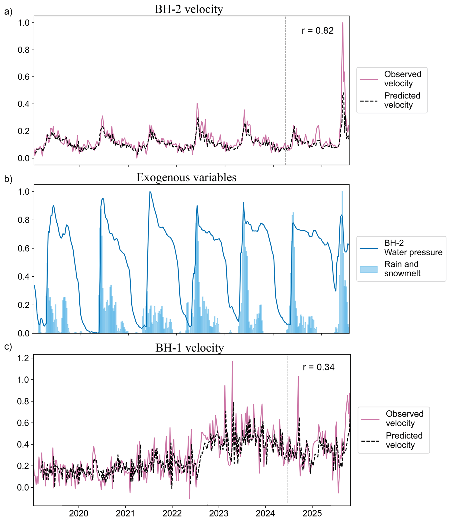
Figure 10 Time series of the analyzed period of the models. Panel (a) shows the observed and predicted borehole BH-2 velocities in the upper shear zone. Panel (b) shows the exogenous variables contributing to the prediction of BH-2. Panel (c) displays the observed and predicted velocities within the shear zone of borehole BH-1. All data are normalized. The vertical dashed line in both plots marks the division between the 80 % training (modeled) and 20 % testing (predicted) periods, and the correlation coefficients shown for the predicted segment.

4 Discussion

4.1 Kinematics of the Jettan and Gámanjunni Landslides

To better understand landslide driving mechanisms in Arctic settings, we compare the kinematics of the Jettan and Gámanjunni landslides. For each site, we compute the mean horizontal displacement across all GNSS receivers to highlight overall kinematic trends and reduce noise, acknowledging that this approach does not capture local variations. Both landslides exhibit similar seasonal patterns: accelerations in spring and autumn, reduced velocities in summer, and a minimum in winter (Fig. 6). Velocity signals are strongly correlated, with Jettan's peak spring acceleration occurring approximately 17 d earlier than Gámanjunni's. The following discussion examines the similarities and differences between the landslides.

At Jettan, spring slip velocities exceed those in autumn, whereas Gámanjunni shows a less consistent pattern, with some years exhibiting higher autumn accelerations. These accelerations correlate strongly with water availability, as indicated by responses to rain and snowmelt in both seasons, suggesting hydrological forcing as a key driver of short-term dynamics. This interpretation aligns with established links between infiltration, groundwater pressure, and landslide displacement (Iverson and Major, 1987). Subsurface thermal conditions differ markedly between the two sites. At Gámanjunni, discontinuous permafrost is inferred from temperature sensors and geophysical observations. Etzelmüller et al. (2022) proposed that spring accelerations may result from meltwater input from ice and snow in fractures. During colder climatic periods, such as the Little Ice Age, permafrost formation at the Jettan landslide was likely (Czekirda et al., 2023). At present, however, the landslide lies below the regional mountain permafrost limit, and evidence from temperature sensors, borehole measurements, and CryoGrid modeling indicates that permafrost is absent. Nevertheless, multi-year ice persists within the backscarp, which may influence hydrological processes by delaying and amplifying infiltration as it melts (Pogrebiskiy and Chernyshev, 1977; Blikra and Christiansen, 2014).

In autumn, infiltration is lower than in spring because snow has melted. Increased slip velocity in autumn correlates with rain events at Jettan, while the relationship is more complex at Gámanjunni. Air temperature and permafrost cooling may influence autumn velocities, as maximum temperature is critical for rock glaciers deformation (Kääb and Røste, 2024) and likely for landslides affected by permafrost (Gruber et al., 2004; Ravanel et al., 2017). Notably, in some years, the annual peak velocity occurs in autumn, suggesting that permafrost may influence seasonal acceleration (Fig. 6).

The Gámanjunni landslide moves three times faster than Jettan. Several factors may contribute to this difference, including geological structural characteristics, slope angle (29° at Jettan and 32° at Gámanjunni), and ground thermal conditions. The landslides occur in different lithological units: Jettan lies within the Nordmannvik Nappe, whereas Gámanjunni is in the Kåfjord Nappe. Jettan consists of garnet–quartz–mica schists with amphibole-rich layers in the lower parts and alternating layers of calc-silicate gneiss and calcite marble in the uppermost parts (Zwaan et al., 2006; Skrede, 2013). Gámanjunni comprises mica schists dominated by biotite relative to muscovite and includes amphibole-rich layers and lenses (Böhme et al., 2016b; Quenardel and Zwaan, 2008). Lithological heterogeneity at Jettan introduces multiple potential weakness zones, whereas the more homogeneous mica schist at Gámanjunni favors the development of a single dominant shear zone. Accordingly, Gámanjunni deforms as a fractured yet largely coherent rock mass along a curved failure plane (Böhme et al., 2016b), in contrast to the Jettan landslide, which exhibits a compartmentalized structure with blocks moving along listric failure planes (Braathen et al., 2004; Blikra et al., 2015). In addition, landslide thickness at Jettan likely shows greater spatial variability than at Gámanjunni, further promoting differential movement (see Figs. 2, 3, and 5). A coherent displacement pattern suggests a more mature landsliding system (Handwerger et al., 2016; Kristensen et al., 2021), evident from displacement vectors following the fall line of Gámanjunni's failure surface at the backscarp, where the block is displaced by 150 m (Böhme et al., 2016b). Comparatively, Jettan's failure surface appears less developed and dips more steeply than displacement vectors, with little vertical offset (Figs. 2 and 5). At Jettan, foliation dips in the same direction as the slope, but at a gentler angle, intersecting the surface downslope. In contrast, Gámanjunni's inward-dipping foliation does not intersect the surface down-slope, implying that outcropping requires a lower-angle sliding surface, likely involving internal deformation or shearing within the rock mass, as indicated by the bulging toe.

Permafrost at the Gámanjunni landslide may contribute to temperature-dependent creep (Krautblatter et al., 2013; Mamot et al., 2018). A long-term relationship has been observed between increasing landslide velocity and rising mean annual rock surface temperature as permafrost thaws (Penna et al., 2023a; Böhme et al., 2019; Hilger et al., 2021). Permafrost is likely absent at Jettan, eliminating this mechanism. In contrast, spatial variability in landslide thickness at Jettan, together with listric sliding surfaces, likely enhances kinematic segmentation and internal deformation, thereby reducing slip rates. A combination of a well-developed shear plane, coherent rock mass movement, and thawing permafrost inside the landslide could be the key factors driving Gámanjunni's faster displacement. However, the role of permafrost cannot be conclusively assessed without borehole data and should be the focus of future investigations.

We interpret that the earlier onset of annual warming at Jettan, due to its lower altitude, leads to earlier snowmelt and infiltration, initiating slip acceleration 17 d before Gámanjunni in average (Fig. 6). This observation highlights that landslides influenced by permafrost and those without permafrost can accelerate at similar times yet exhibit different velocities. Importantly, higher velocities do not necessarily indicate greater hazard. At Gámanjunni, increased velocity may result from temperature-dependent creep, which is unlikely to cause an abrupt failure given the pressure and temperature conditions at the shear-plane depth. In northern Norway, rock slope failures are considerably less frequent than in southern Norway (Penna et al., 2023b). This contrast between active landslides and the absence of historic large-scale slope failures may reflect the stabilizing influence of permafrost or the mechanical properties of mica-rich bedrock, both of which can inhibit rapid failure (Penna et al., 2023a). These same factors may also promote the persistence of active landslides. Although both landslides exhibit comparable surface kinematics, only Jettan has detailed subsurface data, enabling deeper investigation of its seasonal dynamics in the following sections.

4.2 Volumetric Versus Localized Deformation at Jettan Landslide

Subsurface borehole data from the Jettan landslide provide insight into its deformation characteristics. Borehole instruments record displacement along their entire depth, whereas GNSS measures cumulative surface displacement of the whole landslide body. The similar total displacement observed between the two datasets indicates that the boreholes capture the majority of landslide movement.

Borehole data reveal that most displacement occurs within the rock volume rather than along a discrete shear zone, as shown by cumulative displacement profiles in Fig. 5. The Jettan landslide comprises both mica-rich rocks, which are known to exhibit slow creeping behavior (Penna et al., 2023a; Böhme et al., 2013), and alternating layers of gneiss and calcite. This deformation may be facilitated by multiple planes of weakness within the rock mass (Elvebakk, 2013, 2014), enabling distributed strain along structurally weakened pathways (Eberhardt et al., 2004; Rechberger et al., 2021).

Comparable volumetric displacement has been documented at the Åknes landslide in borehole KH-02-06 (Aspaas et al., 2024), which uses the same instrumentation as Jettan. However, newer boreholes at Åknes do not exhibit similar patterns, suggesting that instrument-specific limitations or installation conditions may influence the observed deformation.

4.3 Evolution of Localized Deformation

After characterizing the overall volumetric deformation, we now discuss the development and acceleration of the localized shear zone in borehole BH 1, which exhibits the most pronounced deformation (Fig. 7). Borehole BH-2 upper shear zone and BH-3 are referenced for comparison, while the lower shear zone in BH-2 remains steady during this analysis and is not discussed further.

Prior to the onset of shear-zone accelerations in 2020, 2022, and 2025, displacement in borehole BH-1 was predominantly accommodated within the rock mass. These acceleration phases lead to higher deformation rates and generally coincide with years of deeper snowpacks and more intense snowmelt, with the exception of 2021 (Fig. 2). Although relocation of the Jettan weather station may introduce uncertainty in long-term trends, comparison with the Lyngseidet station shows similar maximum snow depth patterns (Fig. A4), supporting the observed correlation between snow depth and displacement rates. Displacement in borehole BH-1 also correlates moderately with the 14 d running sum of rain and snowmelt, with a 23 d lag, indicating that water infiltration is a key driver. This extended lag may reflect prolonged saturation, possibly linked to shear-plane depth or multi-year ice in the back scarp. Comparable relationships between groundwater pressure and landslide velocity have been documented in other slow-moving landslides (Agliardi et al., 2020; Aspaas et al., 2024; Kristensen et al., 2021; Finnegan et al., 2022). However, open boreholes may not accurately reflect in situ groundwater flow paths or pore-pressure conditions because they can intercept multiple fractures and hydraulically connect otherwise distinct aquifers (Aspaas et al., 2024). As a result, hydraulic conditions observed within the borehole may not represent those in the surrounding rock mass. Furthermore, because the magnitude of water flow along the shear planes is unknown, the relative contributions of seepage forces and pore-pressure effects cannot be quantified. These processes are therefore not considered further in the present analysis.

Initial displacement behavior in borehole BH-1 (Fig. 7) differs from the expected seasonal acceleration pattern. The absence of acceleration phases in the years before 2020 indicates that meteorological forcing alone cannot explain the three acceleration periods. A plausible explanation is structural modification within the shear zone, driven by progressive damage (Eberhardt et al., 2004). ARDL modeling supports this interpretation by identifying the dominant role of endogenous factors in controlling displacement. These findings suggest that internal processes increasingly govern deformation, which is consistent with a maturing and structurally evolving shear zone. This evolution may also explain the increased sensitivity to water infiltration observed in later years. Further evidence emerged after the spring acceleration of 2025, when BH-1 displayed a seasonal acceleration pattern similar to the upper zone in BH-2, characterized by rapid acceleration followed by deceleration.

A notable pattern appears when comparing boreholes BH-1 and BH-3, which are aligned along the landslide slope. Both initially show similar displacement rates, followed by acceleration in 2020. BH-3 then decelerated while BH-1 maintained high velocity. This difference might reflect transient loading associated with strain accumulation and horizontal stress redistribution (Leshchinsky et al., 2019; Lacroix et al., 2020), culminating in a burst of acceleration in BH-3, before slowing. A similar imbalance recurs in 2025, as BH-3 accelerates following an earlier acceleration in BH-1 (Fig. 7). The relationship between these two boreholes is also supported by the ARDL model. Comparable patterns of transient acceleration and strain redistribution have been documented at the Åknes landslide (Aspaas et al., 2024).

The Jettan landslide comprises several individual blocks that exhibit different deformation patterns and hydrological sensitivities. At times, boreholes BH-1 and BH-3 appear mechanically coupled, while at other times they behave independently due to diverging velocities. We infer that the boreholes sample local asperities within a potential plane that is yet to coalesce into one through-going shear zone, where progressive damage modifies mechanical parameters locally, whereas strain imbalances act at a larger scale to influence the overall evolution of the shear zone. The increasing occurrence of simultaneous slip across these asperities suggests a maturing failure surface with an increasing likelihood of sudden failure.

4.4 Rheological Evolution of the Jettan Landslide

Ambient seismic noise analysis reveals a clear cyclical seasonal pattern in apparent seismic velocity changes ($\mathrm{d}v/v$) (Fig. 9). Seismic velocity reductions typically begin in mid-spring and persist until early winter, with two distinct minima in summer and autumn. Because ambient noise is sensitive to changes within the landslide volume, these variations likely reflect changes in water content, temperature, or mechanical rigidity (Larose et al., 2015).

Cross-correlation analysis shows strong negative relationships between $\mathrm{d}v/v$ and shallow ground temperature (1 m depth), the 14 d sum of rain and snowmelt, and borehole BH-1 velocity (Table 2). The long-term cyclicity of $\mathrm{d}v/v$ suggests a similarly fluctuating controlling mechanism. From 2013 to 2020, borehole BH-1 displacement exhibited a predominantly linear, non-seasonal trend, indicating that $\mathrm{d}v/v$ does not directly reflect shear zone stability (Fig. 7). While both shallow temperature and water availability display seasonal signals, only rain and snowmelt exhibit two distinct annual peaks (Fig. 8). Previous studies have shown a $\mathrm{d}v/v$ decreases with wetting (causing stiffness reduction) and increases with drying of the medium (Liu et al., 2024; Borgeat et al., 2025). At the Åknes landslide (fractured gneiss), Bogner et al. (2026) reported $\mathrm{d}v/v$ drops between 2.6 % and 3.9 % associated with water-level increases of several meters at approximately 80 m depth. Here, the first drop in $\mathrm{d}v/v$ (between day 8 and 9 in Fig. 9b) coincides with peak velocities in GNSS and borehole shear zones, whereas the second drop (day 10 in Fig. 9b) aligns with GNSS acceleration but not with borehole acceleration. This pattern suggests that spring acceleration reflects localized shear deformation, while autumn acceleration represents volumetric deformation of the landslide body. Collectively, these observations support an interpretation of an annual rheological transition from rigid to compliant behavior driven by progressive wetting of the landslide.

From a monitoring perspective, 4 % to 7 % decreases in $\mathrm{d}v/v$ have been observed in other landslides prior to collapse (Mainsant et al., 2012; Bontemps et al., 2020) or acceleration (Liu et al., 2024), although such signals are not consistently observed across landslide sites (Borgeat et al., 2025). At Jettan, 4 % drops in $\mathrm{d}v/v$ precede acceleration events, but thresholds proposed in previous studies (Mainsant et al., 2012; Bontemps et al., 2020) or values exceeding two standard deviations, do not appear to serve as reliable precursors to sudden failure in this case. Distinguishing between drying and wetting, as well as isolating landslide failure effects within the expected wetting and drying range (i.e. ±2) is not feasible. However, decreases exceeding 4 % may indicate reduced landslide stability.

A gradual negative trend in $\mathrm{d}v/v$ is observed since 2019. Linear regression indicates a consistent rate of approximately −0.23 % yr⁻¹. This trend may reflect progressive internal changes within the landslide system, such as increased water content or reduced structural integrity, which could facilitate future failure. However, this trend applies only to the observed period and should not be extrapolated, as future environmental or mechanical conditions may alter system behavior.

The seasonal signal in $\mathrm{d}v/v$ provides a valuable proxy for tracking water infiltration within the landslide body. These observations offer a physical explanation for the annual kinematic behavior of the landslide, where water saturation drives a transition from rigid block-like movement to compliant volumetric deformation. This rheological shift highlights the role of hydrological forcing in modulating landslide dynamics on a seasonal basis.

4.5 Synthesis of Landslide Dynamics

The observations presented above indicate that hydrological forcing is the primary control on seasonal acceleration of these Arctic landslides, whereas geological structure and permafrost conditions modulate deformation style and long-term creep rates. Despite contrasting thermal regimes, both landslides exhibit similar seasonal responses to snowmelt and rainfall, while the higher slip velocity and more coherent displacement pattern at Gámanjunni likely reflect a more mature failure geometry and potentially the influence of permafrost-related creep. At Jettan, deformation is distributed throughout the rock mass, and progressive damage together with increasing interaction between localized shear zones suggests ongoing failure-plane development. Ambient seismic noise observations further indicate a seasonally recurring rheological transition associated with water infiltration, linking reductions in material stiffness to a shift from localized shear deformation toward more volumetric deformation. Collectively, these results highlight the coupled roles of hydrology, structural evolution, and thermal conditions in governing the dynamics of Arctic rock slope instabilities.

5 Conclusions

This study compares two Arctic landslides in northern Norway, Gámanjunni and Jettan, separated by only 10 km. At Gámanjunni, geophysical observations indicate the presence of permafrost, whereas Jettan appears to lack it. Despite this difference, both landslides exhibit similar seasonal kinematics, although Gámanjunni creeps roughly three times faster. In Troms county, northern Norway, the widespread occurrence of mica-rich lithologies combined with possible permafrost conditions may contribute to the region's high proportion of active landslides. Subsurface data from Jettan reveal that deformation is controlled by both endogenous and exogenous factors. Local asperities within shear zones likely undergo progressive damage, increasing sensitivity to water infiltration, while strain imbalances across the landslide body drive large-scale shear zone evolution. Apparent seismic velocity changes in the landslide volume further indicate a seasonal transition from localized to volumetric deformation modulated by hydrological forcing.

These findings provide new insights into the controlling processes of Arctic landslides. Water infiltration emerges as the dominant factor controlling seasonal acceleration, while permafrost, where present, may exert an additional control on long-term creep rates. By integrating subsurface observations with surface kinematics, this study strengthens the physical basis of Arctic landslide behavior. Distinguishing between hydrologically driven seasonal accelerations and deformation associated with permafrost thaw enhances landslide hazard assessments by clarifying which slope instabilities are primarily governed by transient hydrological forcing and which may exhibit elevated long-term deformation. Furthermore, these results inform monitoring strategies in warming polar regions by highlighting the need to account for both permafrost conditions and subsurface groundwater dynamics within unstable slopes. In this context, seismic monitoring offers a cost-effective complement to borehole investigations, providing spatially distributed constraints on rock mass mechanical properties rather than relying solely on discrete point measurements.

Appendix A

Section A1 describes the seismic data analysis, supported by Figs. A2, and A5–A11, and Tables A6 and A7. Section A2 provides details of simulated ground temperatures at the location of borehole BH-1 in the Jettan landslide, with Fig. A4 comparing observed and modeled temperatures. Figure A1 validates rolling functions and cross-correlation without introducing artificial lags, while Fig. A3 presents the comparison between the Lyngseidet meteorological station and the seNorge dataset for Jettan. Tables A1–A3 summarize instrumentation at the two landslides and provide additional information on borehole depth and shear zone composition. Tables A4 and A5 summarize the Auto Regressive Distributed Lags (ARDL) models' results.

Monitoring of the Jettan and Gámanjunni landslides has been continuous since instrument installation, with all data recorded and stored by the Norwegian Water Resources and Energy Directorate. These datasets were retrieved and processed as described in the Methods section of the main manuscript. Ground temperature modeling data were obtained from the Norwegian Meteorological Institute (Sect. A2).

A1 Seismic data analysis

This section presents how seismic data were processed to obtain the time series of the variation of the apparent velocity of surface waves ($\mathrm{d}v/v$). This is achieved in two main steps: (1) evaluation of the sensitivity of surface waves as a function of frequency and depth and (2) computation of $\mathrm{d}v/v$ from raw seismic data.

The first step consists of defining a one-dimensional synthetic seismic stratification model. This stage is compulsory to define the frequency range to retain to compute the $\mathrm{d}v/v$ time series in the desired depth range. To evaluate this sensitivity, several geomechanical parameters are required for each subsurface unit, namely their thickness, P- and S-wave velocity (V_P and V_S, respectively) and unit weight (ρ).

Thickness and V_P were retrieved from previous reports: a morphological cross-section (Blikra and Christiansen, 2014) and a seismic refraction profile (Rønning et al., 2008). The location of these profiles is shown in Fig. A5 and they are presented in Figs. A6 and A7, respectively.

The vertical distribution of V_S was determined using two approaches. First, the empirical relationship of Brocher (2005) was tested. It relates V_P and V_S (both in km s⁻¹) to a variety of crustal materials and reads:

$$\begin{array}{}\text{(A1)}& \begin{array}{rl}{V}_{\mathrm{S}}& =\mathrm{0.7858}-\mathrm{1.2344}{V}_{\mathrm{P}}+\mathrm{0.7949}{V}_{\mathrm{P}}^{\mathrm{2}}\\ & -\mathrm{0.1238}{V}_{\mathrm{P}}^{\mathrm{3}}+\mathrm{0.0064}{V}_{\mathrm{P}}^{\mathrm{4}}.\end{array}\end{array}$$

The values obtained are consistent with the geomechanical units in place, with the exception of the strongly fractured rock unit, which provided a too low velocity (285 m s⁻¹). To circumvent this issue, another approach was tested: since all parameters were established, the only remaining unknown is V_S in this unit. Then, it was calculated using a trial and error method using the analytical formula proposed by Dobry et al. (1976). This formula allows for the determination of the resonance frequency f₀ of a subsurface profile using only the thickness and V_S of its different units. The resonance frequency was experimentally determined from measurements of seismic ambient noise at the JETT station and the results are shown in Fig. A8. Approximately 79 000 hourly seismograms between 2016 and 2024 were used to compute the Horizontal-to-Vertical (H$/$V) ratio with the geopsy package (Wathelet et al., 2020). The black curve in Fig. A8 represents the most probable H$/$V curve, with a maximum (but moderate) amplification of around 3 at $f_{\mathrm{H}/\mathrm{V}}=\mathrm{2.5}$ Hz. Assuming that the measured $f_{\mathrm{H}/\mathrm{V}}$ corresponds to the resonance frequency of the first 60 m below ground (10 m of landslide mass plus 50 m of strongly fractured rock; Table A6), V_S in the unit “strongly fractured rock” was adjusted to obtain $f_{\mathrm{0}}=f_{\mathrm{H}/\mathrm{V}}=\mathrm{2.5}$ Hz. This led to V_S=750 m s⁻¹, which is consistent with the other geomechanical parameters of this unit. Finally, unit weight was taken as the median of the measurements obtained by Vick et al. (2021), which are shown in Table A6.

The final 1D geomechanical model in the vicinity of seismic station JETT is presented in Table A7. It was used to compute the sensitivity kernels of surface waves, i.e. their sensitivity as a function of frequency and depth. The computation was conducted using Disba (Luu, 2021), which is a Python package that implements a subset of codes from the Computer Programs in Seismology (Herrmann, 2013). The results are shown in Fig. A9. Figure A9a resumes the 1D synthetic model established previously and Fig. A9b shows the dispersion curves of the fundamental mode of Rayleigh and Love waves corresponding to the synthetic model. Figure A9c and d show the sensitivity kernels of Rayleigh and Love waves, respectively.

Raw seismograms were processed as described in the main text and the present section aims at providing supporting, but non essential information. The daily correlograms for pair of components Vertical-East (Z-E), bandpass-filtered in the range [4.5–6.5] Hz are shown in Fig. A10. The subplot on the right shows the SVD-Wiener-filtered correlograms. The vertical dashed lines represent the limits of the lag time that was used to compute $\mathrm{d}v/v$, between $[-\mathrm{2}:-\mathrm{0.2}]$ and [0.2:2] s, and the reference correlogram is represented as a red curve. This time range allows us to get rid of potential autocorrelation near zero lag and focus on scattered surface waves.

Individual $\mathrm{d}v/v$ time series are presented in Fig. A11. Briefly, curves showing the highest amplitude of variation in both $\mathrm{d}v/v$ and cc are those which encompass the East-West component. This is because it is the main degree of freedom of the landslide mass. The curve at the bottom of the figure corresponds to the average of the three components, weighed by their individual cc, and is the curve used in the paper. This approach has been proposed by Hobiger et al. (2014) and the weighed average $\mathrm{d}v/v$ is obtained using:

$$\begin{array}{}\text{(A2)}& \mathrm{d}v/v\left(t\right)={\displaystyle \frac{{\sum }_{k=\mathrm{1}}^N{\text{CC}}_k^{\mathrm{2}}\left(t\right)\cdot \mathrm{d}v/v_k\left(t\right)}{{\text{CC}}_k^{\mathrm{2}}\left(t\right)\cdot \mathrm{d}v/v_k\left(t\right)}},\end{array}$$

where k is the pair of components, N is the total number of pairs of components (three in this work), CC is the weigh-averaged coefficient of correlation. CC is obtained using:

$$\begin{array}{}\text{(A3)}& \text{CC}\left(t\right)={\displaystyle \frac{{\sum }_{k=\mathrm{1}}^N{\text{CC}}_k^{\mathrm{2}}\left(t\right)}{{\sum }_{k=\mathrm{1}}^N{\text{CC}}_k^{\mathrm{3}}\left(t\right)}}.\end{array}$$

Finally, Fig. A2 shows the complete $\mathrm{d}v/v$ time series from January 2016 to July 2025.

A2 Ground temperature simulation

We applied the CryoGrid community model (Westermann et al., 2023) to simulate ground temperature along a vertical profile at borehole BH-1 of the Jettan landslide to fill gaps in the observational data. We modeled a 1D column from the ground surface to a depth of 130 m, considering altitude and slope angle, provided by the Digital Elevation Model at the borehole location.

We used a time series of NORA3 (Haakenstad et al., 2021; Haakenstad and Breivik, 2022) [data retrieved from The Norwegian Meteorological Institute] as forcing data, spanning from 1965 to 2023 with a 3 km resolution. The data were downscaled following the topoSCALE routine implemented in CryoGrid (Fiddes and Gruber, 2014), and bias-corrected for air temperature using a day-of-year quantile mapping approach (Themeßl et al., 2012) with in-situ observations from the meteorological station at Jettan (Fig. 2, main text). To extend the time series back to 1850, monthly mean anomalies from CESM2 (Danabasoglu et al., 2020) were applied to the NORA3 data. The simulations covered the time period from 1850 to 2023, with the first 10 years serving for the accelerated spin-up (Westermann et al., 2023). Only the time period from 1 September 2019 to 1 September 2023 was used for further analysis.

The model domain was defined by two stratigraphy classes, each with specific physics describing the thermal state and water/ice balance. In the upper five meters, the stratigraphy class GROUND-freezeC-bucketW-seb was used to calculate the surface energy balance, soil freezing characteristics after (Painter and Karra, 2014), and the water balance based on a bucket scheme, meaning that soil water is retained within the soil matrix, or it moves downwards due to gravitational forces (Westermann et al., 2023). Removal of surface water was based on the Gauckler-Manning equation. Below five meters depth, we applied the stratigraphy class GROUND-freeW-seb, which simplified the freezing characteristics to a phase change of water at 0 °C, and water and ice contents to a constant sum. The surface albedo was set to 0.15, and the surface roughness to 0.01 m. With bedrock characterizing the soil profile, a porosity between 5 % and 7.5 %, and a field capacity of 0.03 were specified.

Seasonal snow was represented by the Crocus-based snow class (Vionnet et al., 2012), considering wind compaction, initial snow density, and varying surface albedo. A snowfall factor multiplied with the forcing data allowed for the representation of local differences in snow accumulation.

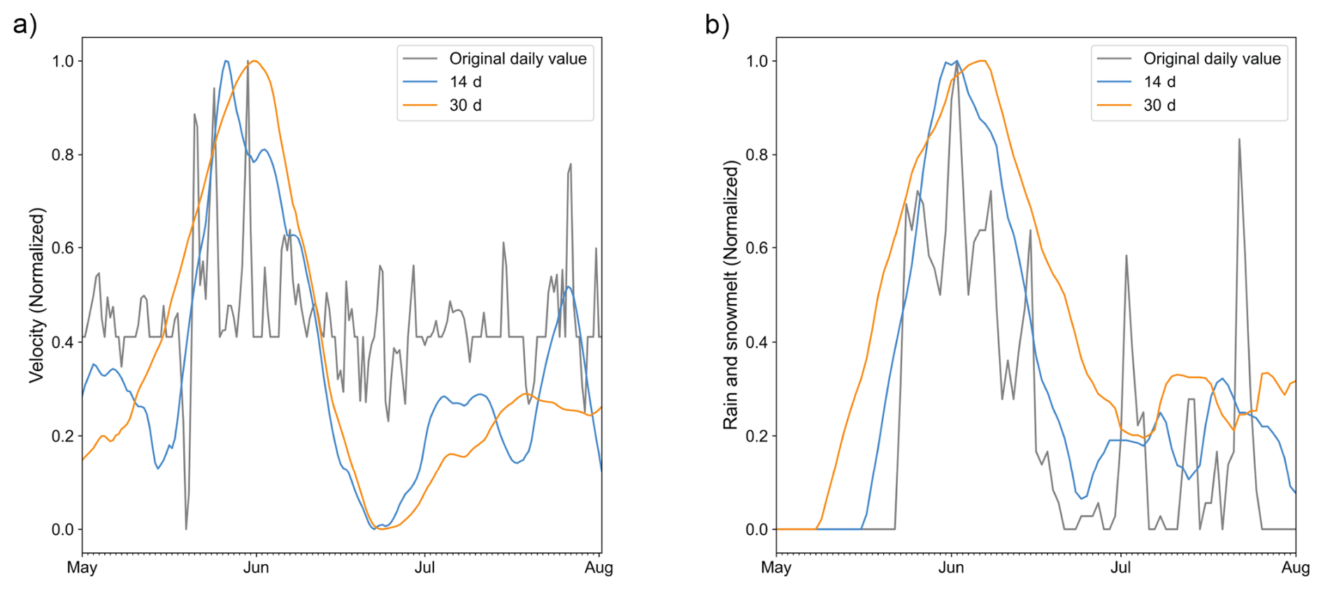
Figure A1 Verification of zero lag created by the window lengths by the rolling functions. (a) Normalized velocity from GPS-4 on Jettan with 1, 14, and 30 d velocity calculated by the centered rolling linear regression function (see Section Integration of Data). (b) Normalized rain and snowmelt summed over 1, 14, and 30 d by the centered running sum function.

To address uncertainties in rock characteristics and snow accumulation, we ran the model with 12 varying parameter sets: porosity of 5 % or 7.5 %, thermal conductivity of 2.8 or 3.0 W mK⁻¹, and snowfall factors of 1, 1.1, or 1.2. The median value across all scenarios was taken for analysis. The model results were validated against observational data from borehole BH-1 and showed good agreement at different depths. In the year 2023, at 115 m depth, a ground temperature of 2.20 °C was measured, while the model simulated 2.23 °C. At 45 m depth, the measured temperature was 1.86 °C, compared to the simulation result of 1.72 °C. At the ground surface (Fig. A4), the simulation could capture the seasonal temperature signal, particularly during snow-free conditions, when movements in the landslide occur. Larger discrepancies were observed during the snow season, which can be traced back to a poor representation of individual snowfall events and snow redistribution in the complex terrain of Jettan, which goes beyond the model's capacities.

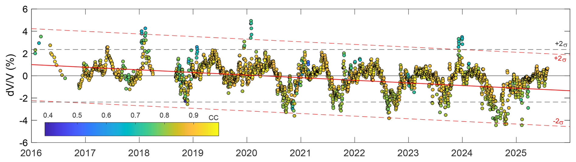
Figure A2 Daily $\mathrm{d}v/v$ time series (not smoothed) computed between 4.5 and 6.5 Hz, which corresponds to the time series presented in the main text. The color scale refers to the coefficient of correlation between the reference and each daily correlograms. Horizontal dashed lines stand for the 95 % confidence interval between −2 and 2σ (with $\mathit{\sigma }=\pm \mathrm{1.18}$ %). The red line represents the linear trend of the time series with an annual decrease of 0.23 %, and the red dashed lines the corresponding 95 % confidence interval (with $\mathit{\sigma }=\pm \mathrm{1.6}$ %).

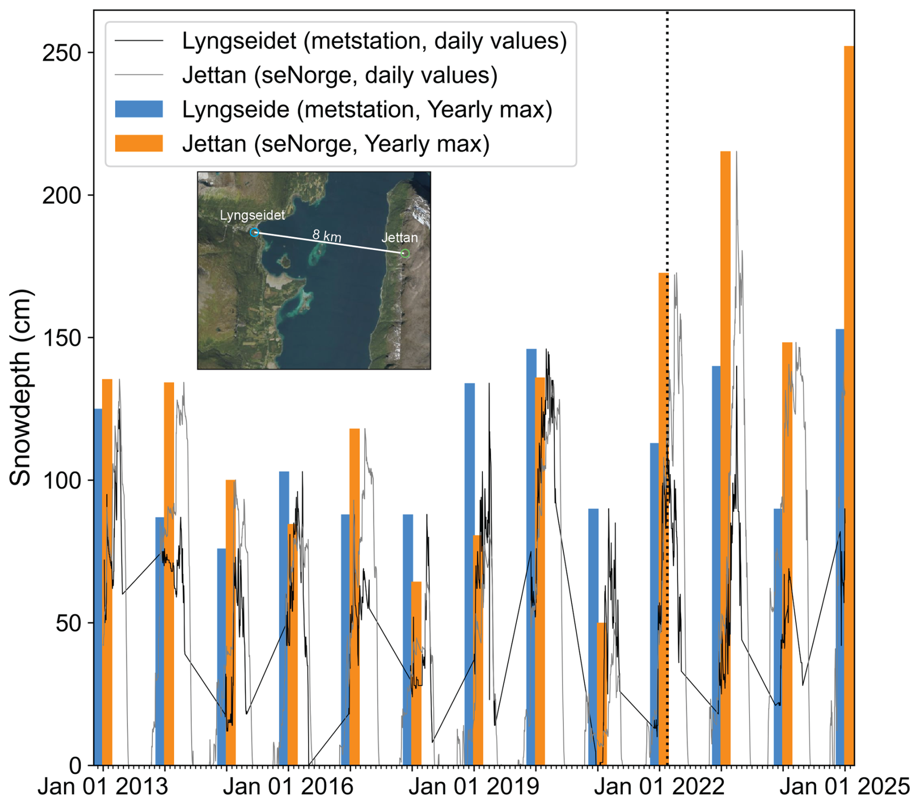
Figure A3 Daily snow depth values from the Lyngseide meteorological station across the fjord from Jettan and the seNorge modeled dataset. More snow could be accumulating on the new station as we see an increase after 2022 in the seNorge dataset and no such increase at the Lyngseide station (seNorge data courtesy of seNorge).

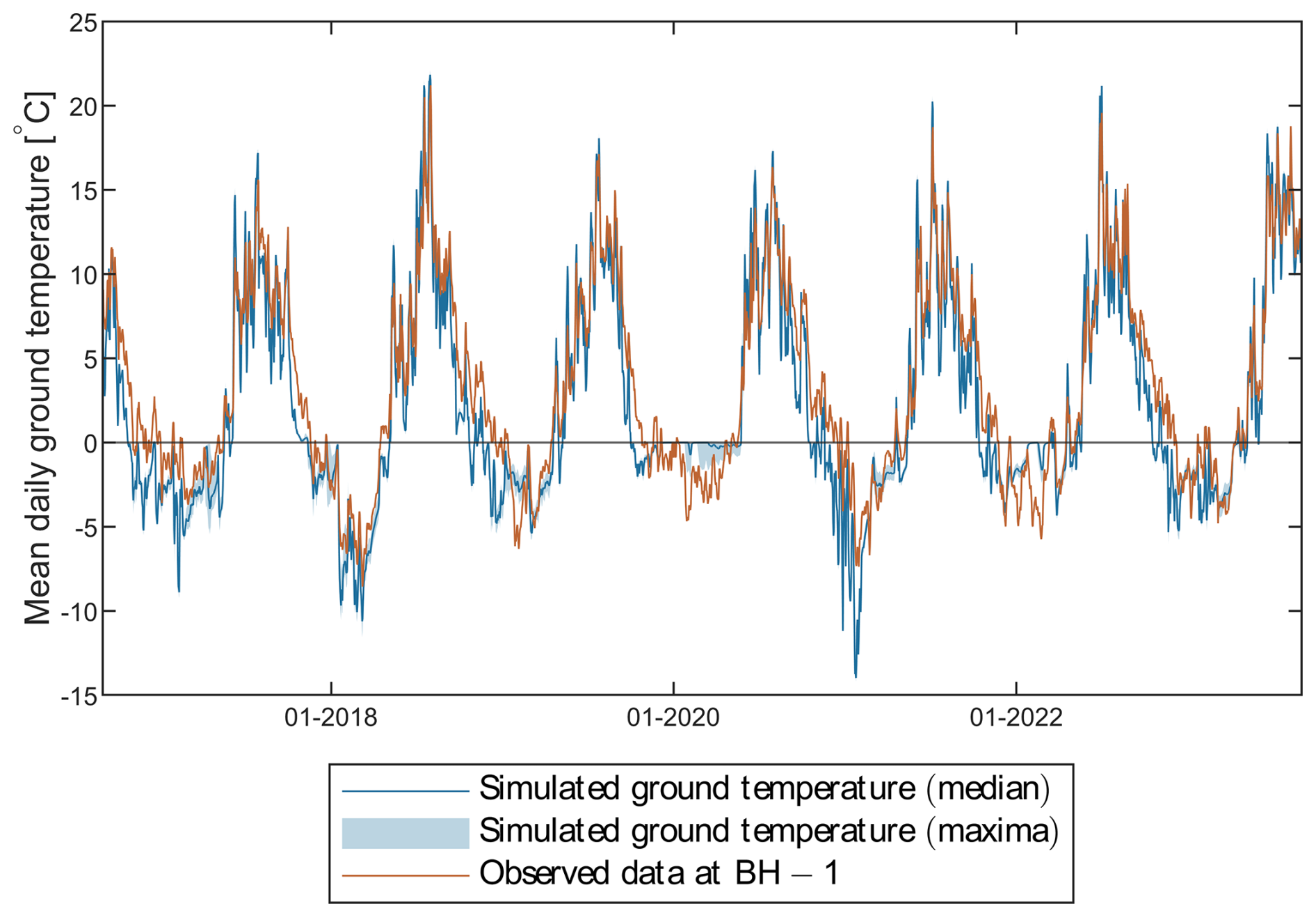
Figure A4 Simulated and observed ground temperatures at one meter depth in borehole BH-1 in the Jettan landslide. The simulations include 12 varying parameter sets to account for uncertainties in the bedrock characteristics and snow dynamics. The model setup is described in Sect. A2.

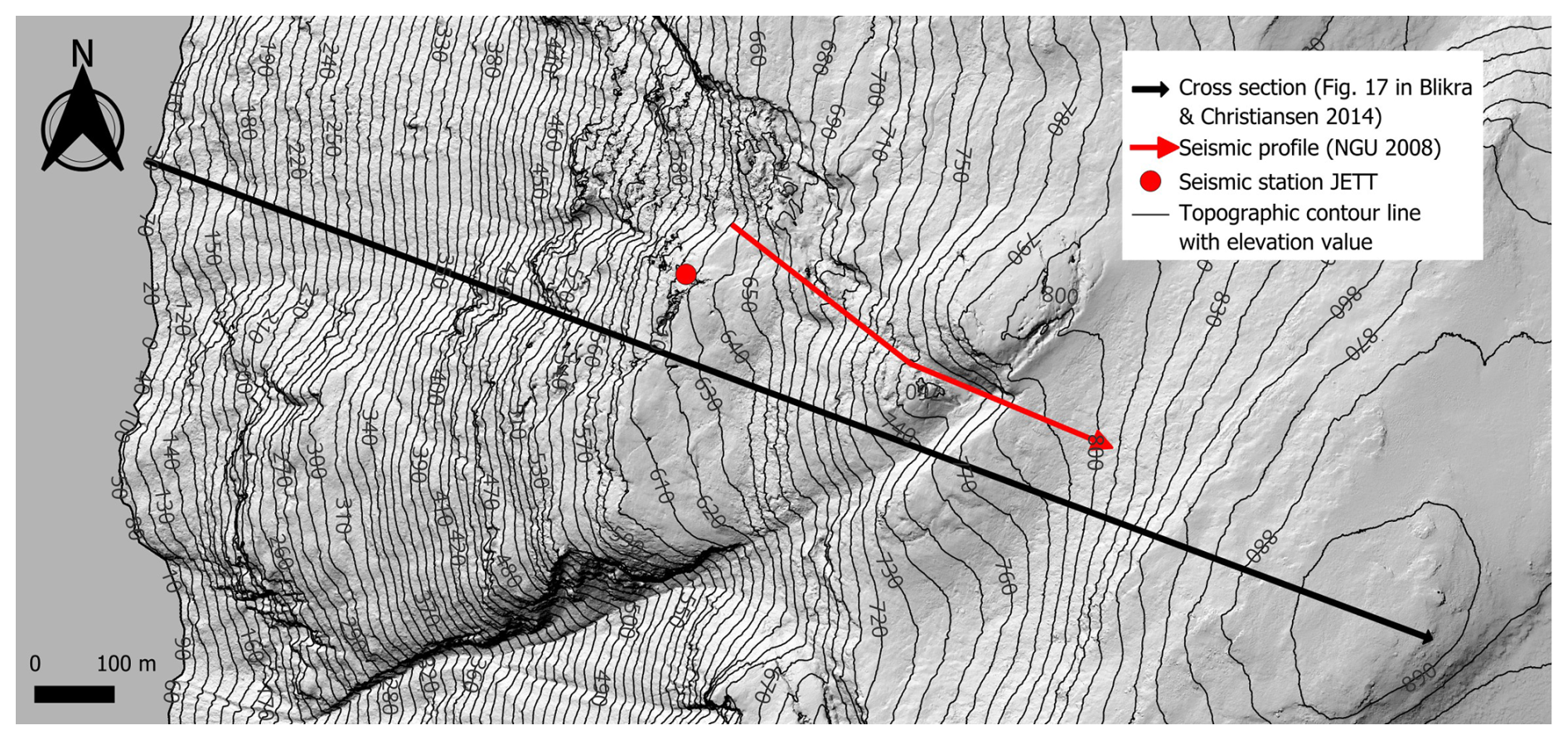
Figure A5 Location of the seismic measurements. The black arrow represents the cross-section presented in Fig. A6.

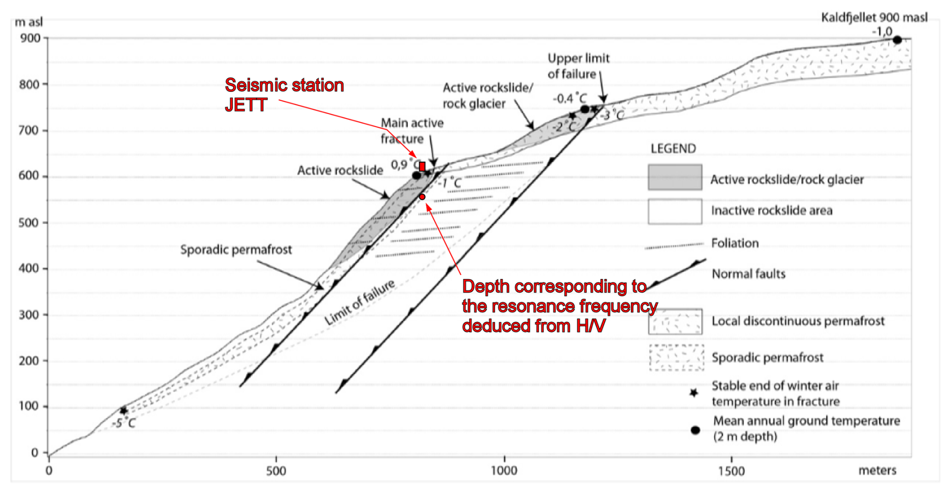
Figure A6 Profile of the Jettan rockslide, modified from Blikra and Christiansen (2014).

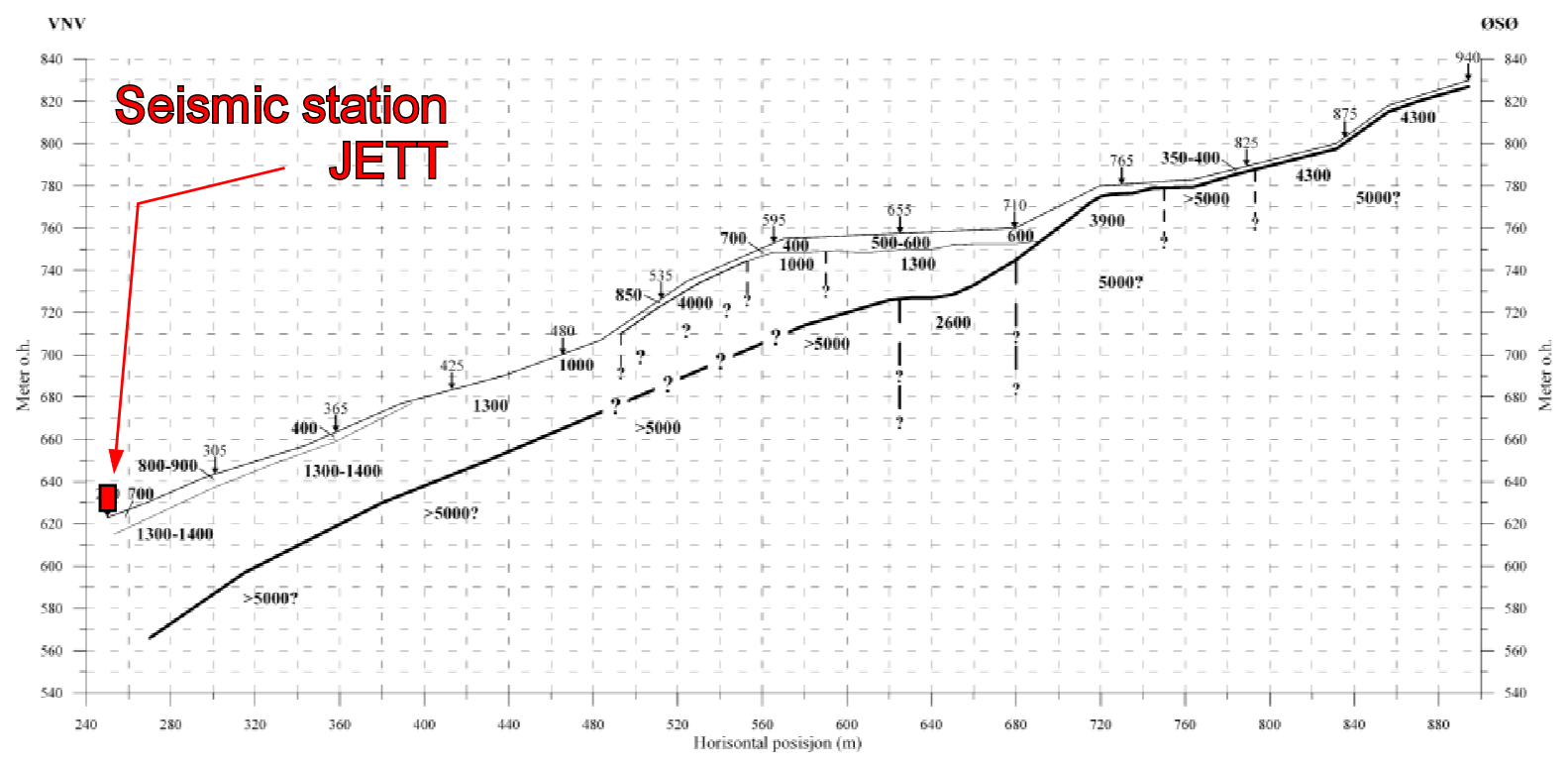
Figure A7 Seismic refraction profile in the upper part of the Jettan rockslide (Rønning et al., 2008). The location of the profile is shown in Fig. A6.

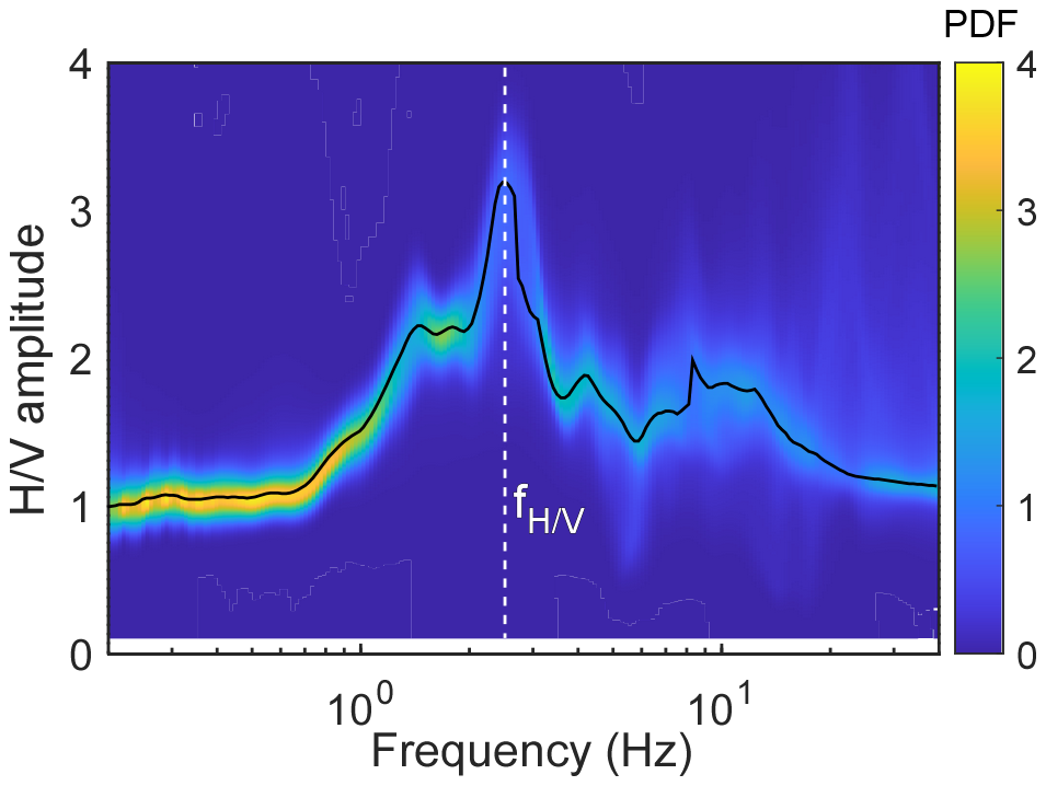
Figure A8 The average H$/$V curve at seismic station JETT. The probability density function (PDF) was established using around 79 000 hourly curves between 2016 and 2024. The black curve represents the maximum PDF. The white dashed line shows a maximum (but moderate) amplification of around 3 at frequency $f_{\mathrm{H}/\mathrm{V}}=\mathrm{3.5}$ Hz.

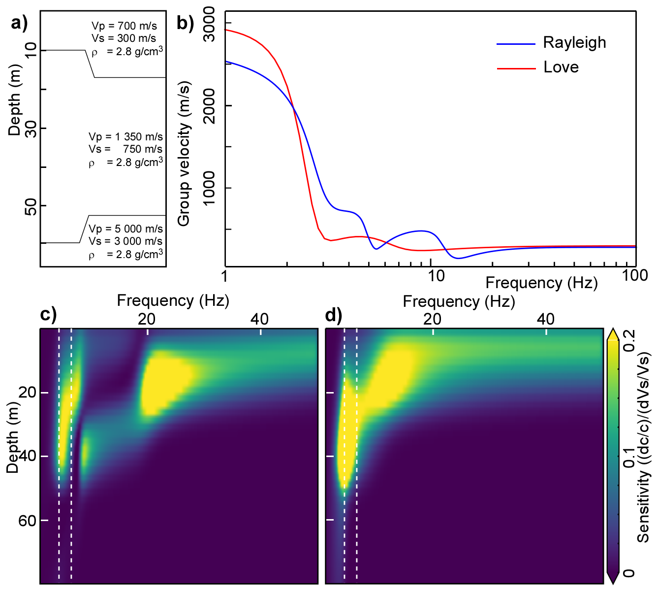
Figure A9 Sensitivity kernels of surface waves at the Jettan rockslide. (a) Seismic stratification. (b) Theoretical dispersion curves of the fundamental modes of Rayleigh and Love waves. (c, d) Sensitivity of Rayleigh and Love waves, respectively, as a function of depth and frequency. The white dashed lines represent the frequency range (4.5–6.5 Hz) used in the paper.

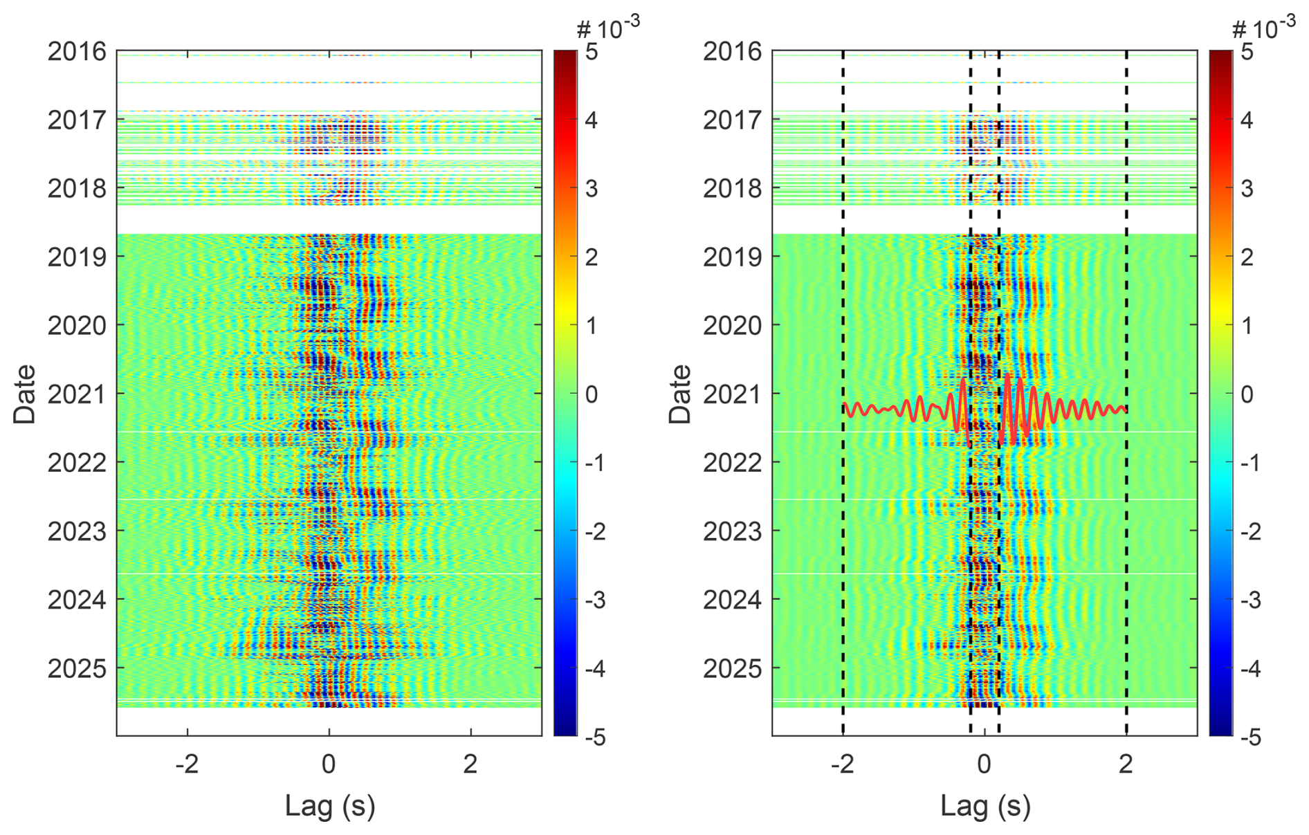
Figure A10 Daily correlograms at Jettan between vertical and east-west components, and filtered between 4.5 and 6.5 Hz. Left: Raw correlograms. Right: Correlograms after the Wiener-SVD filtering (Moreau et al., 2017). The vertical dashed lines represent the time range ($[-\mathrm{2}:-\mathrm{0.2}]$ and [0.2:2] s) used for computing the $\mathrm{d}v/v$ time series.

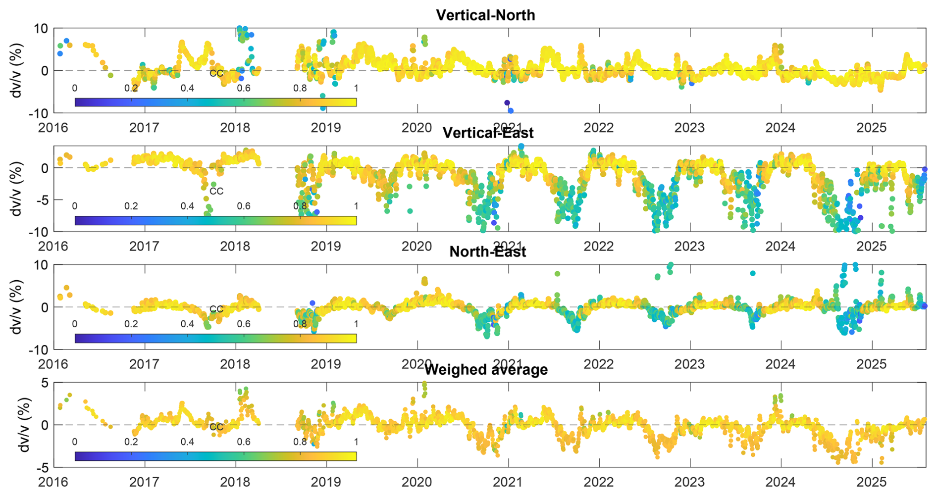
Figure A11 Time series of $\mathrm{d}v/v$ at seismic station JETT on Jettan landslide. The first three graphs show individual time series for the three possible pairs of components Vertical-North (Z-N), Vertical-East (Z-E) and North-East (N-E). The graph at the bottom shows the average $\mathrm{d}v/v$ time series where each $\mathrm{d}v/v$ value is weighed by its coefficient of correlation.

Table A1 Table of instruments installed on the Jettan landslide by type, product name, number of devices, installation date, analyzed period, acquisition frequency, and measurement resolution provided by the manufacturer.

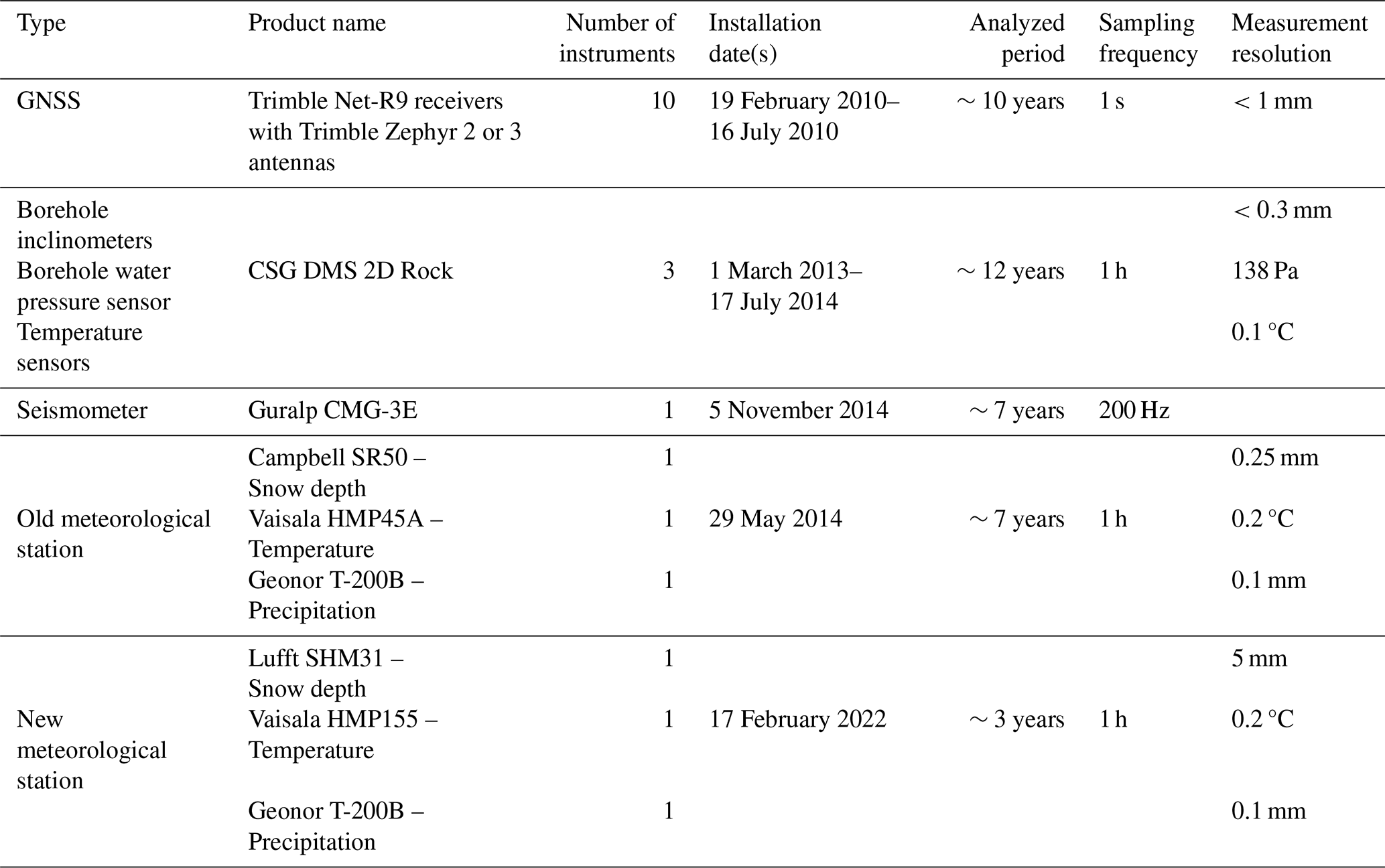
Table A2 Table of instruments installed on the Gámanjunni landslide by type, product name, number of devices, installation date, analyzed period, acquisition frequency, and measurement resolution provided by the manufacturer.

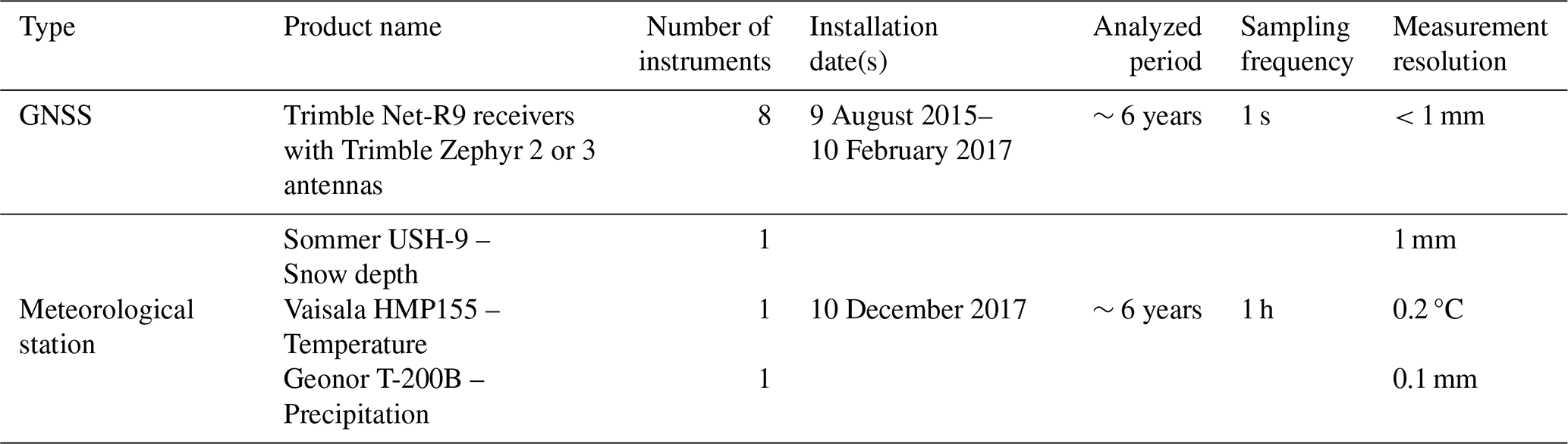
Table A3 Table of boreholes installed at the Jettan landslide, displaying the detection period, shear plane depth, material composition of the shear zone, and the total instrument depth.

The shear plane column indicates boreholes that intersect both an upper and a lower shear plane, whereas boreholes with one shear plane are left blank. ^a Ganerød (2013). ^b Ganerød (2014).

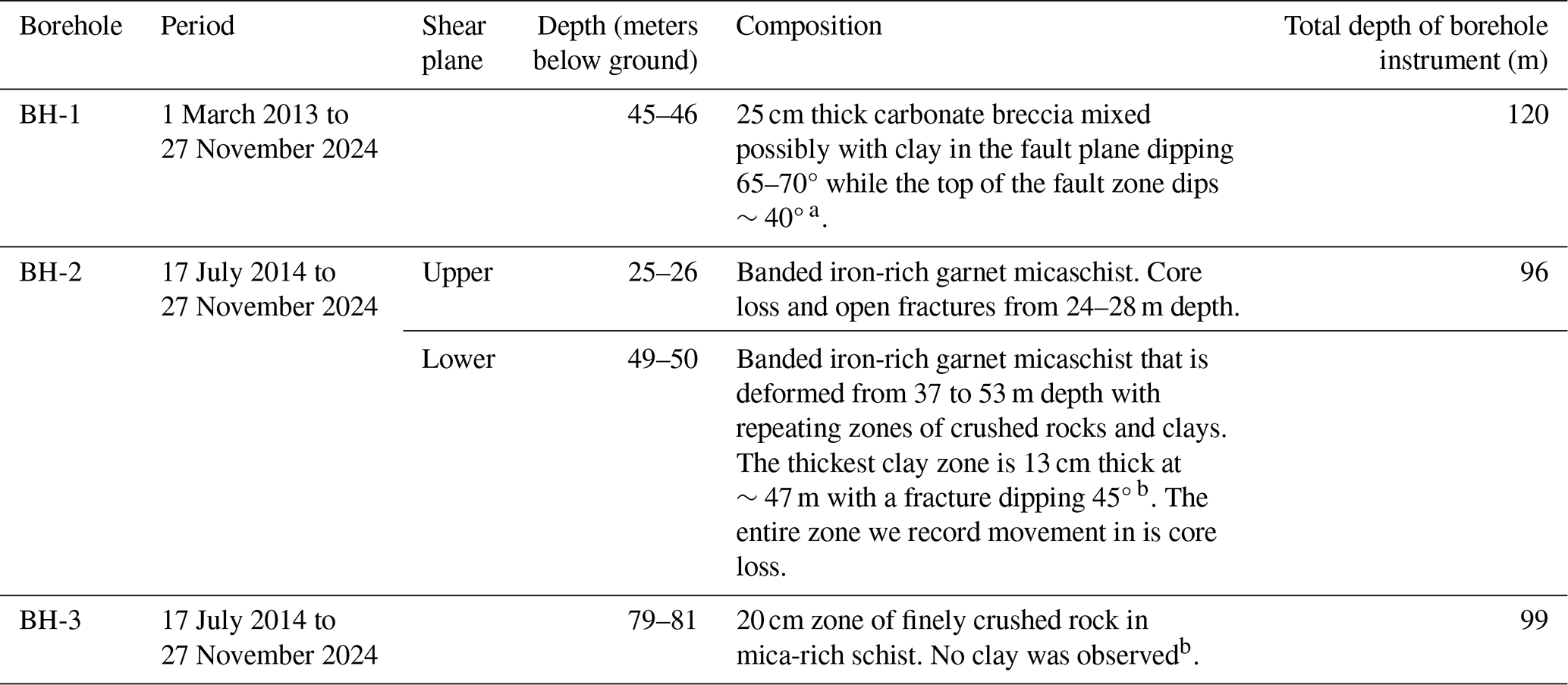
Table A4 Autoregressive Distributed Lag (ARDL) model (see Eq. 2 in the main text) results for the upper shear zone in borehole BH-2. The table lists endogenous and exogenous variables included in the model, with their lag order denoted as variable_name.Ln. For each term, the estimated coefficient (α for autoregressive terms and β for distributed lag terms) is shown along with its statistical significance (p value). Larger absolute coefficients indicate a stronger influence on the modeled sliding velocity. The variable names are: BH-2 (borehole BH-2), BH-2_WP (borehole BH-2 water pressure), Air_temp (air temperature from seNorge), Rain_Snow (total precipitation from rain and snowmelt from seNorge), and $\mathrm{d}v/v$ (relative seismic velocity change).

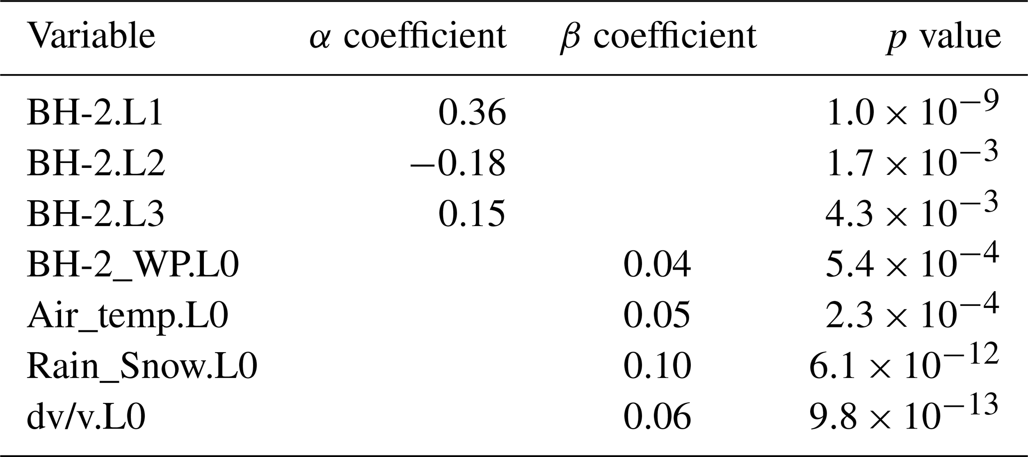
Table A5 ARDL model results (see Eq. 2 in the main text) for the shear zone in borehole BH-1. The table lists endogenous and exogenous variables included in the model, with lag order indicated as variable_name.Ln. For each term, the estimated coefficient (α for autoregressive terms and β for distributed lag terms) is shown together with its p value, with statistically significant terms shown in bold. Larger absolute coefficients suggest a stronger influence on sliding velocity within the model. Variable names: BH-1 (borehole BH-1) and BH-3 (borehole BH-3).

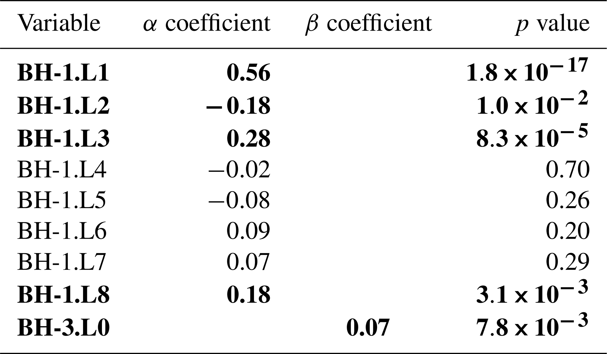
Table A6 Geomechanical parameters of the lithological units (Vick et al., 2021).

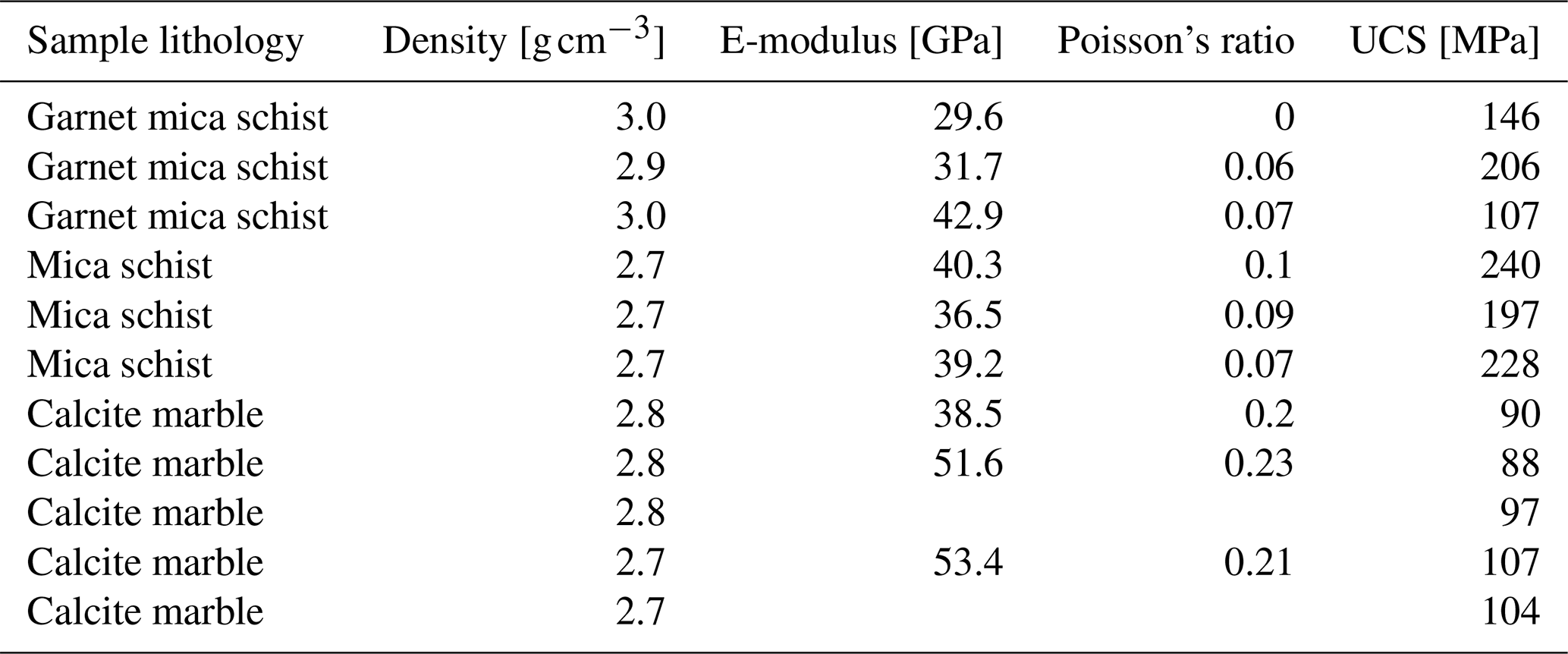
Table A7 Geomechanical and seismic model used for the computation of the sensitivity kernels. Terminology of the units after Rønning et al. (2008). V_p: P-wave velocity; V_s: S-wave velocity.

^a Evaluated from empirical relationships (see text for details). ^b Evaluated from a trial and error approach (see text for details).