TopoToolbox 3, a laboratory for quantitative geomorphology

TopoToolbox has been widely used to analyze and model landscapes across geomorphology and other geospatial disciplines for the past 15 years. Its documentation and accessible interfaces have made it a valuable resource for teaching and learning quantitative geomorphology while its customizability and efficiency have allowed researchers to use it as a platform for experimentation and implementation of their own analyses and models. Its third version, TopoToolbox 3, builds on these developments by improving access to the software, integrating with a larger ecosystem of geomorphology software, and establishing sustainable research software engineering practices. TopoToolbox, previously available only in MATLAB, is now also available to users of Python, and an R interface is under development. The redesigned architecture of TopoToolbox 3 is based on a shared library of core computational routines that makes these and other integrations possible while maintaining the MATLAB interface for existing users of the software. We illustrate the power of this design with examples of how users can integrate TopoToolbox into their workflows. First, we compare the implementation of a basic application, χ maps, in MATLAB and Python. Second, we show how property-based testing can successfully identify bugs in the absence of known solutions to test cases. We then use the GraphFlood hydraulic model, now available in TopoToolbox, to showcase the potential of integrating simulation tools and analyzing their output in one computational environment. Finally, we demonstrate a two-way coupling between TopoToolbox and the Python-based Landlab landscape evolution modeling framework. We conclude by discussing how improved quality assurance and community-driven development practices ensure that TopoToolbox continues to serve the evolving needs of the geomorphology community.

1 Introduction

TopoToolbox (Schwanghart and Kuhn, 2010; Schwanghart and Scherler, 2014) is a software platform for research in quantitative geomorphology. It provides data structures for representing gridded digital elevation models (DEMs) and flow networks derived from them, as well as tools for manipulating, analyzing and visualizing these data structures. The software has been widely used for research not only in terrestrial geomorphology and hydrology (Ward et al., 2019; Wainwright et al., 2022) but also in marine geomorphology (Bernhardt and Schwanghart, 2021, 2025) and planetary geology (Arakawa et al., 2020) and in other geospatial sciences such as glaciology (Culberg et al., 2022; Van Wyk de Vries et al., 2023; MacKie et al., 2021; Kneib et al., 2024; Karlstrom and Yang, 2016), volcanology (Tennant et al., 2023), soil science (Hunter et al., 2024) and ecology (Wainwright et al., 2020; Bertrand et al., 2021; Val et al., 2022; Falco et al., 2024) to name a few. This popularity has been attributed to user-friendly interfaces, extensive documentation including an active blog (https://topotoolbox.wordpress.com, last access: 6 November 2026), and its computational efficiency. Many tools have also been built on top of TopoToolbox, using its data structures to implement more specific analyses or to provide different user interfaces (Campforts et al., 2017; Gallen, 2017; Forte and Whipple, 2019; Tangi et al., 2019; Steer, 2021; Tennant et al., 2023).

TopoToolbox's dependence on MATLAB (The MathWorks Inc., 2022) has been critical to its success. MATLAB provides an integrated development environment, an interactive visualization system and its own extensive documentation. Users can download MATLAB and TopoToolbox and immediately begin using the software. However, while TopoToolbox itself is open source and freely available, it requires a license for MATLAB as well as several additional toolboxes that provide both essential functionality (Image Processing and Mapping Toolboxes) and important additional functions (Optimization Toolbox). Many other software tools for quantitative geomorphology also exist from topographic analysis packages similar to TopoToolbox such as Whitebox (Lindsay, 2016) and LSDTopoTools (Mudd et al., 2019), to landscape evolution modeling frameworks such as Landlab (Hobley et al., 2017; Hutton et al., 2020; Barnhart et al., 2020) and Fastscape (Bovy and Lange, 2023), to standalone analytical tools such as TopoMetricUncertainty (Smith et al., 2019), pyTopoComplexity (Lai et al., 2025) or CliffDelineaTool (Swirad and Young, 2022), to complete GIS platforms like ArcGIS and QGIS (Dawson et al., 2026) and programming languages like Python, R and Julia, and these represent only a fraction of the many software tools that researchers use to study the Earth's surface (Grohmann et al., 2026). Each of these tools provides a unique combination of analyses and user interfaces that may serve a user better than TopoToolbox, but if a user of one of these tools wishes to access an analysis available in TopoToolbox or if a TopoToolbox user wishes to integrate one of these tools into their workflow, they can face challenges interfacing between the different computational environments.

Nevertheless, users do often combine TopoToolbox with a variety of other tools. For example, Gillen et al. (2025) used TopoToolbox to delineate drainage basins before loading this data set into ArcGIS, where they compared the drainage basin areas to digitized reef shorelines. MacKie et al. (2021) used TopoToolbox alongside the MATLAB-based Antarctic Mapping Tools (Greene et al., 2017) to compute subglacial flow paths over topography that was simulated with S-GeMS, a specialized geostatistical software package (Remy, 2005). Culberg et al. (2022) used TopoToolbox to compute flow accumulation while using QGIS for additional DEM processing and several MATLAB-based tools for radar data processing. Such workflows import data into each tool, process it, then export the results for use in the next program. This pattern works well for analytical pipelines, in which data can be processed once, exported and stored for later use. It is less well-suited for interactive data analysis or modeling that requires the repeated exchange of data between tools. Moreover, while some data such as gridded raster datasets have standard file formats that can be read and written using libraries like GDAL (GDAL/OGR contributors, 2025), Python's rasterio (Gillies et al., 2013), MATLAB's Mapping Toolbox, or R's terra (Hijmans, 2025), other data, such as flow and stream networks, do not have these standardized formats and are more complicated to exchange between tools.

The main innovation of the most recent release, TopoToolbox 3, is the introduction of a software architecture that makes it easier to combine with other tools, to make the software accessible to more users, and to establish a sustainable, community-driven, development process in accordance with the FAIR Principles for Research Software (Barker et al., 2022). In comparison to previous releases, TopoToolbox 3's major added value is its multi-layer architecture and a software development framework including automated testing, regular releases, and a contribution process that invites community involvement in the future development of the software.

The major change visible to users is the introduction of a Python package (Kearney et al., 2026b), which provides a similar interface to the MATLAB package and enables users to integrate TopoToolbox with Python-based tools including geomorphology research software like Landlab. This package uses a new C library, libtopotoolbox (Kearney et al., 2026a), which implements core functionality shared across higher-level languages. The MATLAB package (Kearney et al., 2026d) has been modified to use libtopotoolbox while ensuring backward compatibility with previous versions. Users of the previous MATLAB version should notice only minor changes to the interface. TopoToolbox 3's multi-layer architecture also facilitates its integration into other tools. An R package (https://github.com/TopoToolbox/topotoolboxr, last access: 6 November 2026) and a QGIS plugin (https://github.com/TopoToolbox/QGISTopoToolbox, last access: 6 November 2026) are actively being developed, and the community is encouraged to develop TopoToolbox 3 integrations for their own tools. A new GitHub organization (https://github.com/TopoToolbox, last access: 6 November 2026) coordinates the development of TopoToolbox, and contributions to any of the organization's packages can be made through a pull request workflow described in more detail in the organization's Contribution Guidelines (Kearney, 2026).

This paper illustrates and evaluates the approaches taken to develop TopoToolbox 3. We describe how TopoToolbox is split into a computational core and binding layers, and how the object-oriented user interface implemented in previous versions is applied in other programming languages. In addition, we describe the testing framework and how to overcome the challenge of testing terrain analysis software where correct answers for a given input are not necessarily known. Finally, we present four practical examples using TopoToolbox 3. We illustrate how a typical geomorphological analysis workflow differs across the MATLAB and Python implementation. We evaluate TopoToolbox's testing framework with an example of how tests caught a real bug in libtopotoolbox. We demonstrate the value of using TopoToolbox as a development platform for new analyses in computational geomorphology with the GraphFlood hydrodynamic model (Gailleton et al., 2024). Finally, we integrate TopoToolbox with Landlab to show how the new architecture enables intermodel comparisons and compare the results and performance benchmarks to highlight opportunities for the future development of geomorphological software tools. This manuscript focuses on the design decisions and software development practices that make TopoToolbox 3 possible. While we do present practical examples of TopoToolbox 3's use for scientific analyses, this is not intended as a tutorial or instructional guide on TopoToolbox 3, and some understanding of the underlying algorithms and the geoscientific reasoning behind them is assumed. The online documentation available at https://topotoolbox.github.io (last access: 6 November 2026) and especially the examples gallery at https://topotoolbox.github.io/gallery (last access: 6 November 2026) contain more detailed instructional material, including fully worked versions of the examples presented herein, and we encourage users and potential users of TopoToolbox to look there for guidance and inspiration.

As the scope of TopoToolbox has expanded with this new version, its name has unfortunately become somewhat overloaded. In this manuscript, we use “TopoToolbox” to refer generally to the software, especially when discussing its conceptual framework, the organization that coordinates its development and the community of users and developers who support it. “TopoToolbox 3” is used when referring specifically to the design, implementation and functionality of the newest version of TopoToolbox in contrast to that of “TopoToolbox 2”, the MATLAB package described by Schwanghart and Scherler (2014). Whereas TopoToolbox 2 was a single, self-contained MATLAB package, TopoToolbox 3 consists of several separate components. The MATLAB and Python packages released as part of TopoToolbox 3 are themselves each called TopoToolbox within their respective languages and documentation, but they are hosted in GitHub repositories called “topotoolbox3” and “pytopotoolbox” to avoid name collisions. Those names are occasionally used in this manuscript to distinguish between the two packages and to refer to the GitHub repositories where necessary. “libtopotoolbox” refers to the C library and its repository.

2 Methods

TopoToolbox 3 was designed to achieve three goals – integrating more smoothly with existing software, improving accessibility and encouraging community engagement with the software – while operating under the constraints of backwards compatibility with TopoToolbox 2 and portability across programming languages and operating systems. We first describe the architecture of TopoToolbox 3 and how it addresses these goals and constraints. We then discuss the testing and quality assurance methods that provide confidence in an increasingly complex software system. Finally, we present four examples that illustrate the functionality of TopoToolbox 3, its quality assurance framework and its integration with external software.

2.1 Architecture and design decisions

The architecture of TopoToolbox 3 consists of three layers (Fig. 1). The C library libtopotoolbox provides shared functionality to packages that provide a high-level user interface in MATLAB and Python. A language-specific binding layer (pybind11 and MEX) exchanges data between libtopotoolbox and the higher-level packages. Data input/output and visualization are the responsibility of libraries such as rasterio and the Mapping Toolbox in the higher-level language. The common core of libtopotoolbox ensures that essential computational routines are available across multiple languages. Relying on the same underlying library in different languages means that the results are reproducible regardless of the language used and reduces the sensitivity of TopoToolbox's results to changes in its dependencies.

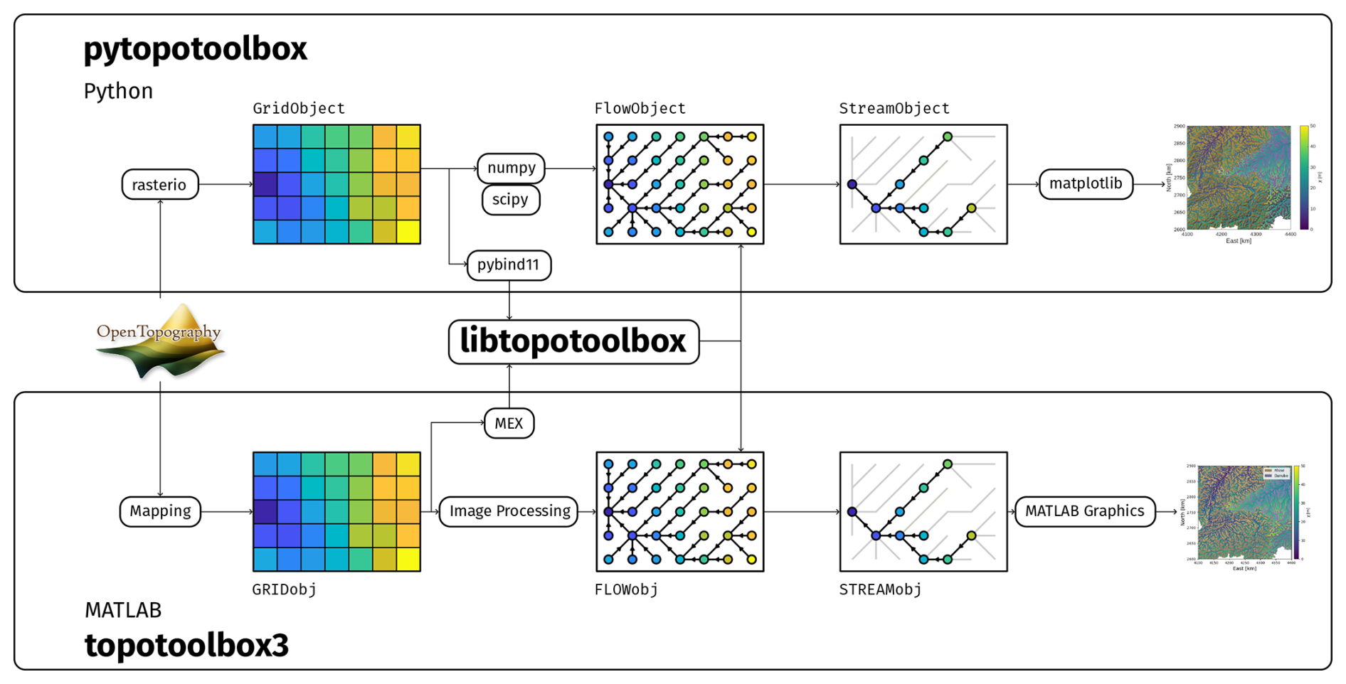
Figure 1 A hypothetical workflow using TopoToolbox 3 illustrates its architecture. Packages provided by TopoToolbox 3 (shown in bold font) include interfaces in high-level languages (pytopotoolbox, topotoolbox3) and the core library (libtopotoolbox). Digital elevation models can be downloaded from services like OpenTopography or loaded from disk into a Grid object. Flow routing over this DEM creates a Flow object. Language-specific array and image processing libraries are used along with libtopotoolbox to accomplish flow routing and other algorithms. The binding layer (pybind11, MEX) exchanges data between the high-level languages and libtopotoolbox. A subset of the Flow object, the Stream object, represents the stream network. These objects can be plotted using language-specific visualization libraries.

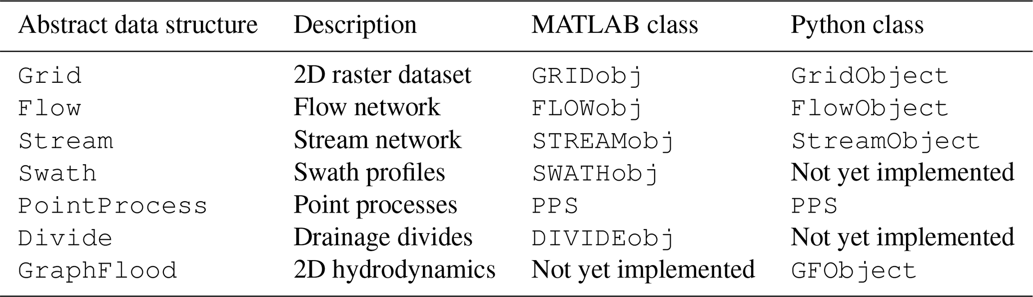
The high-level interfaces to TopoToolbox 3 preserve the object-oriented approach developed for TopoToolbox 2 (Schwanghart and Scherler, 2014). Three major classes provide functionality: Grid objects represent DEMs and other gridded data sets. Flow objects represent the flow directions, and Stream represent a stream network as a subset of the DEM connected via the flow directions (Table 1). These objects have different names in MATLAB and Python (GRIDobj/GridObject, FLOWobj/FlowObject, and STREAMobj/StreamObject) and the language-agnostic terms Grid, Flow and Stream are used here unless the specific implementation in MATLAB or Python is discussed. Much of the core functionality available in the MATLAB package for each of these three objects has been added to the Python package as well, but complete feature parity between the two interfaces has not yet been achieved. The MATLAB package also includes the additional classes of SWATHobj for extracting swaths of DEMs and DIVIDEobj for analyzing drainage divides (Scherler and Schwanghart, 2020), but these have not yet been ported to the Python package. The PPS object for analyzing point processes on stream networks (Schwanghart et al., 2021) is available experimentally in Python. The GraphFlood algorithm is currently accessible from the run_graphflood function in both Python and MATLAB, but the Python interface to the GraphFlood algorithm has been encapsulated in a GFObject class, which provides additional options that are not yet available in MATLAB.

Table 1 The correspondence between classes in TopoToolbox 3 in MATLAB and Python.

libtopotoolbox implements a data-oriented approach (Fabian, 2018) in which its functions operate only on contiguous arrays of data supplied by the functions' caller. This avoids the complexity of managing object representations and ownership within the C library and enables libtopotoolbox to be used with any language that provides a foreign function interface to C and the ability to access contiguous arrays. Methods in the high-level language extract the necessary arrays from the Grid, Flow and Stream objects before passing them to libtopotoolbox, and they package the output arrays into objects to be returned to users. Some methods like Grid.fillsinks or Flow.flow_accumulation return raster datasets of the same shape and size as the input DEM, so these are returned as Grid objects that can be used in other TopoToolbox functions.

Other methods, especially those of Stream objects, return one-dimensional (1D) MATLAB or Numpy arrays. These are either node attribute lists with an element for every node in the stream network or edge attribute lists with an element for every edge between two nodes of the stream network. Quantities like the distance upstream from an outlet or χ are attached to nodes and thus returned as node attribute lists. Quantities like the distance between two nodes or the fraction of flow apportioned to two downstream neighbors by a multiple flow direction routing algorithm are attached to edges and returned as edge attribute lists. Stream objects maintain an additional mapping between the indices of its 1D node attribute lists and those of its parent Grid object, which can be used to extract information from Grid objects at the nodes of the stream network using the Stream.ezgetnal method.

The Flow and Stream objects represent flow networks with a topologically sorted edge list as in TopoToolbox 2 (Hergarten and Neugebauer, 2001; Braun and Willett, 2013; Schwanghart and Scherler, 2014). This data structure stores the links between nodes in the flow network in an order such that all incoming edges to a node occur before any outgoing edges. The edge list consists of two arrays, each of which contains integers labeling the source and target of each edge in the flow network. Many network analysis algorithms can be implemented succinctly with one or more scans of the topologically sorted edge list, and the uniform representation of flow and stream networks as topologically sorted edge lists means they can share libtopotoolbox implementations for many of their functions. libtopotoolbox contains a set of functions that use flow algebras (Tarboton and Baker, 2008) to compute various quantities of interest such as drainage area, downstream and upstream distance and χ.

libtopotoolbox functions are not typically called by users. Instead, methods on Grid, Flow and Stream objects initialize the necessary input and output arrays and pass them to libtopotoolbox through the binding layer. The binding layer marshals data between the high-level language and libtopotoolbox, converting the high-level language's data representations into the contiguous arrays of data needed by libtopotoolbox. TopoToolbox 3 uses MATLAB's MEX system and pybind11 (Jakob et al., 2017) for the Python bindings. Additional C or C++ source code within the MATLAB and Python packages implements these bindings.

libtopotoolbox currently focuses on in-memory processing of data to make as few assumptions as possible about where a user's data comes from. A DEM loaded into memory in MATLAB using the Mapping Toolbox or in Python using rasterio or created by a landscape evolution model can all be passed to libtopotoolbox functions. The user decides how and when to load their data into memory. This design does make it challenging to operate on DEMs too large to load entirely into memory. Existing solutions for processing large DEMs require control over the input and output of data tiles and communication across the boundaries of tiles (e.g. Arge et al., 2003; Barnes, 2016, 2017). Implementing these algorithms in libtopotoolbox would require users to access their data through libtopotoolbox instead of the libraries they are already using, which is contrary to the design goal for libtopotoolbox to operate on as wide a variety of data sources as possible. Such solutions could, however, be implemented in TopoToolbox's higher-level packages using libraries like dask (Rocklin, 2015) or MATLAB's Parallel Computing Toolbox to orchestrate I/O tasks and libtopotoolbox to perform computations on each tile. An alternative that is also being considered is to reimplement the libtopotoolbox interface using hardware acceleration frameworks such as the Parallel Computing Toolbox in MATLAB or Taichi Lang, PyTorch and TensorFlow in Python that provide access to resources like multiprocessors and GPUs. In this case, the high-level interface would remain the same, but users could switch between between the portable libtopotoolbox backend and high-performance backends as needed. Work is ongoing to leverage these libraries to provide an easy-to-use, high-performance interface for analyzing large datasets.

2.2 Testing and quality assurance

The manual testing performed for TopoToolbox 2 is not able to provide the level of quality assurance required to ensure that code behavior is preserved across languages, that interfaces between high-level languages and libtopotoolbox continue to work correctly after changes in one or both layers, and that the software works properly with external packages. An extensive automated testing system has been implemented for TopoToolbox 3. Each TopoToolbox package contains an automated test suite that runs using a language-specific testing framework. Pull requests submitted to the repository trigger runs of the test suite on GitHub Actions to verify the changes proposed in the pull request. The test suites are run on recent versions of Linux, Windows and macOS, and the Python and MATLAB package repositories run their test suites with the supported versions of Python (3.10 and newer) and MATLAB (R2023b and newer). All changes to TopoToolbox repositories are made through pull requests, and no changes are accepted unless the test suite passes.

A major challenge in testing scientific software is the oracle problem or the need to know the correct answer for a given input (Barr et al., 2015). While oracles can be constructed for small test cases and analytical solutions to many algorithms are available, we want to ensure that TopoToolbox gives correct results on real data, not just these hand-crafted data sets, which may not capture edge cases or unexpected features of real data. The TopoToolbox 3 test suites use the following techniques to create realistic test cases.

2.2.1 Snapshot-based characterization testing

Regression tests ensure that changes introduced in TopoToolbox 3 do not substantially affect the behavior of the software. However, the desired behavior of many of the functions of TopoToolbox is not always clearly specified, especially around problems such as the handling of missing data or boundary conditions. We use characterization tests (Feathers, 2004, p. 186) to document the existing behavior of TopoToolbox functions by running a set of real and simulated DEMs through the functions in the MATLAB package and storing the result. The libtopotoolbox and pytopotoolbox test suites download these pairs of input and output data, process the input with their own implementations of the same functions, and then check that their outputs are equivalent to the stored MATLAB outputs up to some small threshold to account for platform-specific differences in floating point arithmetic. In cases where the existing functionality needs to be changed, the snapshot data can be updated using the new behavior.

2.2.2 Property-based testing

Snapshot tests only verify that the behavior of TopoToolbox 3 functions matches their behavior from TopoToolbox 2, not that the implementations are correct. An effective way to test the correctness of these implementations is through property-based testing (Goldstein et al., 2024). Property-based testing specifies software functionality through properties that should hold after some input data is passed through a function. It then verifies that these properties hold when evaluated on randomly generated inputs. For example, the fillsinks function should have the property that the filled DEM no longer has any sinks, i.e. pixels surrounded by neighbors with higher elevations, while drainagebasins has the property that the downstream neighbor of a given pixel should receive the same basin label as that pixel. The test suites randomly generate DEMs and then verify that these properties hold after passing them to the relevant functions.

The fillsinks and drainagebasins functions both depend globally on the DEM. It is impossible to know by looking only at a pixel and its immediate neighbors whether that pixel is part of a sink or to which drainage basin it belongs. However, these properties can be quickly verified by local computations that examine each pixel and its immediate neighbors. Properties that locally test global functions are particularly effective in developing tests because they are easy to write and quick to run, and they discriminate well between correct and incorrect implementations of the function. Local computations such as the gradient8 function, which computes the maximum downward slope between a pixel and its eight neighbors in the DEM, require testing code that is very similar to that of the computation itself. Such a property-based test is less effective at verifying the behavior of the function because bugs in the implementation are likely also present in the test. In the end, it provides as much information as a snapshot test does, ensuring only that the behavior of gradient8 is preserved during changes to the code, and the snapshot test is much simpler to implement correctly. Hand-crafted test cases can be used alongside snapshot tests to verify functionality in these cases.

2.2.3 Metamorphic testing

The major difficulty in implementing property-based tests is the need to generate properties that are testable and that sufficiently distinguish between correct and incorrect answers. Metamorphic testing (Chen et al., 2018) has been a valuable strategy for generating properties for TopoToolbox 3. Metamorphic testing relies on so-called metamorphic relations between multiple inputs to a function and their expected outputs. While the output of each function for a given input may not be known, the difference between the outputs obtained from transformed versions of the inputs can be deduced from a metamorphic relation. Particularly valuable are invariants, aspects of the output that do not change when the input data is modified in a certain way. A simple example of an invariant metamorphic relation in DEM analysis is that the magnitude of the gradient of a DEM should be identical to the magnitude of the gradient of the same DEM rotated by multiples of ninety degrees. Any violation of this metamorphic relation indicates that the gradient implementation depends on the specific arrangements of the x and y axes, which is likely a bug. An example of a noninvariant metamorphic relation obeyed by the gradient function is that the gradient should be proportional to the inverse of the cell size. A test of this relation constructs two Grid objects with identical data but different cell sizes, h₁ and h₂, passes them to the gradient function to obtain two Grid objects, g₁ and g₂, and verifies that the ratio of the gradients is approximately the inverse ratio of the cell sizes ($g_{\mathrm{1}}/g_{\mathrm{2}}=h_{\mathrm{2}}/h_{\mathrm{1}}$) for all pixels with nonzero gradient. A violation of this metamorphic relation indicates that the gradient implementation does not use the supplied cell size correctly.

2.3 Practical evaluation of TopoToolbox 3

To demonstrate how the design of TopoToolbox 3 enables users to incorporate it into various geoscientific workflows, we present four examples. The first example demonstrates how functionality existing in the previous version TopoToolbox has been adapted to TopoToolbox 3 by presenting MATLAB and Python implementations of χ maps and evaluating the consistency of results obtained with the two packages. The second example illustrates how a testing strategy known as metamorphic testing was able to catch a subtle bug in libtopotoolbox. The third example presents GraphFlood (Gailleton et al., 2024), a recently developed hydrodynamic model that has been ported to TopoToolbox 3. Finally, the fourth example demonstrates a two-way coupling between TopoToolbox 3 and Landlab that uses TopoToolbox both to implement a process component of a landscape evolution model and to analyze the model's output. Code samples have been included for some of the examples, but they have been condensed for space. Complete Jupyter notebooks and MATLAB Live Scripts implementing these examples can be found on the online TopoToolbox gallery (https://topotoolbox.github.io/gallery, last access: 6 November 2026).

2.3.1 χ maps

χ maps provide a graphical illustration of the potential for dynamic reorganization of river basins (Willett et al., 2014). They display the value of the χ metric (Perron and Royden, 2013) at points within the stream network. χ is a coordinate transformation that arises when solving the steady-state stream power equation by separation of variables. It is obtained by integrating upstream the inverse of the contributing area (Eq. 1)

$$\begin{array}{}\text{(1)}& \mathit{\chi }=\underset{x_{\mathrm{b}}}{\overset{x}{\int }}{\left({\displaystyle \frac{A_{\mathrm{0}}}{A\left(x\right)}}\right)}^{\frac{m}{n}}\mathrm{d}x\end{array}$$

where A₀ is a reference area, A(x) is the contributing area at each point x in the stream network, which begins at a location corresponding to base level x_b. and m and n are the parameters of the stream power model. When the along-stream coordinate is transformed to χ, stream profiles that solve the steady-state stream power model appear as straight lines whose slope is controlled by the ratio of uplift rate to erodibility.

To conduct a χ analysis in TopoToolbox, the basic workflow is to (1) load a raster containing elevation data, (2) route flow over the topography to determine drainage directions and drainage areas for each cell in the elevation data, (3) identify the stream network from these drainage directions, and (4) perform the upstream integration of drainage area to compute χ.

We have implemented a χ analysis of the Rhine-Danube drainage divide in southwestern Germany and northern Switzerland following that of Winterberg and Willett (2019). The code in both MATLAB and Python used for this analysis is displayed in Fig. 2. This workflow is similar in structure to that depicted in Fig. 1.

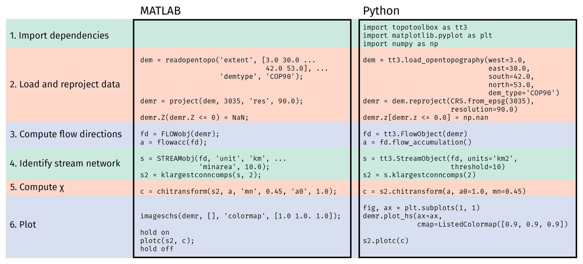
Figure 2 The code used to generate the χ maps. The left column shows the code in MATLAB and the right column the code in Python. The background colors group related sections of the code together. Some details, especially of plotting, have been omitted from the code sample in the interest of space. Complete working examples can be found in the TopoToolbox gallery (MATLAB: https://topotoolbox.github.io/gallery/notebooks/matlab/alpine-chimaps/alpine_chimaps.html, last access: 6 November 2026 and Python: https://topotoolbox.github.io/gallery/notebooks/python/alpine-chimaps/alpine-chimaps.html, last access: 6 November 2026), and the code and necessary auxiliary data to run the examples can also be obtained from the gallery GitHub repository (https://github.com/TopoToolbox/gallery, last access: 6 November 2026).

The Copernicus Global DEM (European Space Agency, 2024) is first obtained from OpenTopography using a TopoToolbox function to call the OpenTopography API. This DEM is loaded into TopoToolbox as a Grid object, TopoToolbox's representation of raster datasets and projected into the ETRS89-LAEA coordinate system with a resolution of 90 m. While many of the algorithms implemented in TopoToolbox can work properly in geographic coordinate systems, their implementations have often assumed that a projected coordinate system is used, and we recommend projecting DEMs when possible to avoid problems. Work is ongoing to ensure functions work in geographic coordinate systems and to document when a function assumes a particular coordinate system. Pixels below 0 m in elevation are replaced by NaN to exclude them from the analysis and set a common base level. A Flow object, TopoToolbox's representation of flow directions, is created from the gridded DEM using the default settings, which route flow using D8 (O'Callaghan and Mark, 1984) with least cost auxiliary topography carving (Schwanghart et al., 2013) through depressions and flat regions. The upstream area is computed using the flowacc/flow_accumulation methods on the Flow objects. A Stream object containing the subset of the flow network identified as stream channels is then generated from the Flow object by applying a minimum upstream area threshold of 10 km². This stream network covers the entire region spanned by the DEM, so it is restricted to the Rhine and Danube basins using the klargestconncomps method to select the two largest drainage basins. Finally, the χ transform is computed from the flow accumulation raster using the chitransform method. The output of chitransform, c, is an array with an element for each node of the stream network giving the χ value computed for that node. The Stream.plotc method is used here to plot this array in geographic coordinates with its value represented by its color, but Stream.plotdz could also be used to plot the stream network elevation against c in the classic χ plot (Perron and Royden, 2013).

2.3.2 Metamorphic testing

To illustrate how TopoToolbox uses property-based and metamorphic testing to ensure that its components work together, we demonstrate a bug in libtopotoolbox's flow routing implementation that was identified by metamorphic testing. This bug was resolved in libtopotoolbox pull request #186 (https://github.com/TopoToolbox/libtopotoolbox/pull/186, last access: 6 November 2026).

The bug has its origins in the memory layout of Grid objects. The two-dimensional (2D) raster data sets that underlie the Grid objects are stored in memory as a 1D array. The data are organized within this array according to either a row- or a column-major layout. A row-major layout puts all the values for a single row next to each other in memory in order of increasing column index. The next row is placed directly after that and the next row after that. The column-major layout puts all the values for a single column next to each other in memory in order of increasing row index. Indexing into a 2D array converts the row and column indices into a linear offset depending on the array's dimensions and the memory layout, and high-level array languages do these conversions automatically.

However, MATLAB arrays are column-major while Numpy arrays are row-major by default but can also be column-major. To operate efficiently on arrays originating from both MATLAB and Python, libtopotoolbox needs to know some information about the memory layout of the 2D arrays supplied as inputs and outputs. Metamorphic tests in pytopotoolbox ensure that this interface is correct by generating two GridObjects with the same data but with different memory layouts, passing both GridObjects to the same function, and checking that the outputs are equivalent.

2.3.3 GraphFlood

Representing streams as networks of flow directions as in TopoToolbox's Flow and Stream objects is efficient for large-scale analysis but lacks detailed hydrodynamic information such as channel width, flow depth, velocity or shear stress that may be useful for investigations of landscape evolution and natural hazards (Davy et al., 2017; Armitage, 2019). Recovering this information can be done by modeling the 2D or even three-dimensional (3D) flow of water over a landscape. However, the computational cost of solving the full shallow-water equations makes them unsuitable for large-scale exploratory analyses. To circumvent this, Gailleton et al. (2024) developed GraphFlood, a numerical method that leverages graph theory and simplified shallow-water equations to compute large-scale, 2D steady-state flow conditions efficiently.

To illustrate how GraphFlood operates within TopoToolbox 3, we simulated flow in the Saison watershed in the Western French Pyrenees using the 25 m BD ALTI DEM (Institut national de l'information géographique et forestière (IGN), 2024). This watershed has a high variability in both relief and valley width, which demonstrates GraphFlood's versatility in estimating flow over different terrain. We estimate flood extent across the entire catchment under three different hydrological states, prescribed in the model by effective precipitation rates of 10, 50, and 100 mm h⁻¹. We then use tools from TopoToolbox 3 and the Python numerical ecosystem to extract and quantify spatial variations in channel width, shear stress, and hydraulic slope near the main trunk under the 50 mm h⁻¹ precipitation scenario.

2.3.4 Integration with Landlab

Landlab is an environment for modeling Earth surface dynamics (Hobley et al., 2017; Hutton et al., 2020; Barnhart et al., 2020). It provides a framework for constructing and running models on a variety of spatial grids as well as an extensive library of “components” that implement different process models or analyses using data on these grids.

The Python interface to TopoToolbox 3 makes it possible both to conduct online analysis of Landlab model results and to use TopoToolbox 3 to represent processes within a Landlab model. We have created an example that uses TopoToolbox 3 in these two roles within a basic landscape evolution model based on an example available in the Landlab documentation (Wickert and Gasparini, 2026). The model represents erosion with a stream power incision model and linear diffusion on hillslopes using Landlab's StreamPowerEroder and LinearDiffuser components, respectively. We replace Landlab's FlowAccumulator, which is used to compute the upslope drainage area needed by the stream power model, with a custom component using the flow routing functionality of TopoToolbox 3, TT3FlowRouter (Fig. 3).

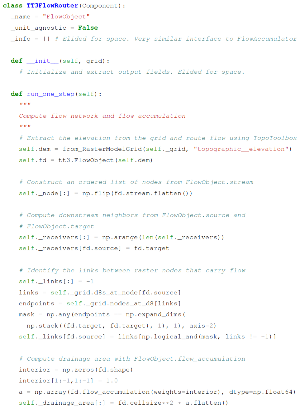
Figure 3 The TT3FlowRouter class. Some details have been removed for clarity and space. See the accompanying Jupyter notebook for complete working example.

TT3FlowRouter is essentially a FlowObject modified to expose the information that Landlab's StreamPowerEroder requires. Landlab represents data as a collection of fields associated with a grid. It provides many different structured and unstructured grid types, but since TopoToolbox focuses on processing regular rasters, we use Landlab's RasterModelGrid with equal horizontal spacing exclusively. A pytopotoolbox GridObject is roughly equivalent to a single node-based field on a RasterModelGrid, and the two can easily be converted from one to another, taking care that the underlying arrays are shaped appropriately for the two different libraries. A helper function from_RasterModelGrid (not shown) is used to create a GridObject from a specified field of a RasterModelGrid in the example.

The gridded data is then run through TopoToolbox's default flow routing algorithm, D8 with morphological carving (Schwanghart et al., 2013). The topologically sorted list of flow network nodes and downstream receivers of each node are readily available from the FlowObject and the drainage area is computed with the flow_accumulation method on FlowObject. The StreamPowerEroder also requires a field containing the labels of the edges that carry flow between nodes of the DEM. Every adjacent pair of nodes in the grid is connected by a “link” in Landlab, whether or not any flow is transported across that link. TopoToolbox, on the other hand, only maintains the list of edges that carry flow, so the edge labels of TopoToolbox do not directly correspond to the link labels of Landlab. We construct this field by manipulating Landlab's list of links in the raster grid and TopoToolbox's lists of the source and target indices of each flow network edge.

At each time step, the TopoToolbox flow routing component is run on the DEM to compute flow directions and flow accumulation, which are supplied to StreamPowerEroder to compute the erosion. The hillslope diffusion is applied by Landlab's LinearDiffuser component and uplift is applied manually to the interior nodes. After 2×10⁶ years of simulated time, the uplift rate is doubled to create knickpoints that propagate upstream. We use TopoToolbox's knickpointfinder to identify these knickpoints (Stolle et al., 2019), and we visualize them on both a hillshaded DEM and a χ plot (Perron and Royden, 2013) created with TopoToolbox's plotting functionality.

3 Results

Here, we present the output of the four examples and discuss each example within the context of the goals of TopoToolbox 3.

3.1 χ maps

Figure 4 shows the pair of χ maps of the region generated in MATLAB (Fig. 4a) and Python (Fig. 4b).

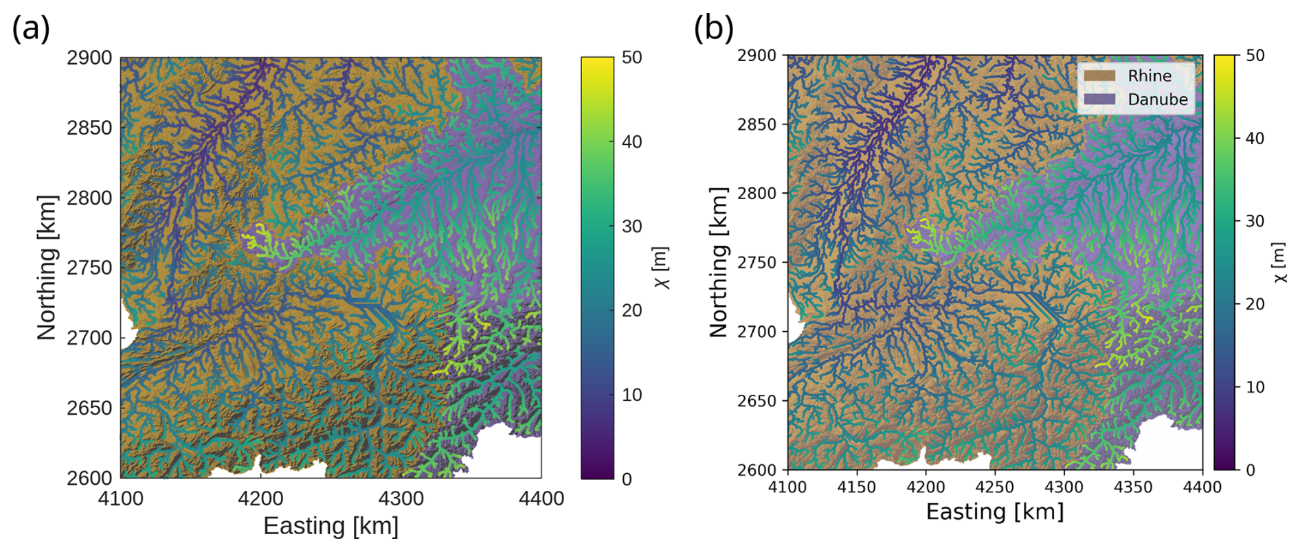
Figure 4 χ maps using TopoToolbox 3. (a) The χ map created by the MATLAB code in Fig. 2. The Danube basin is highlighted in purple and the Rhine in orange. The stream network is colored based on the χ value at each point along the channel. (b) The same figure as (a) created in Python using the code in Fig. 2.

The TopoToolbox workflow is essentially identical in Python and MATLAB, but the two languages and their TopoToolbox implementations are different and users will have to translate between the two when porting code from one language to another. For example, the two languages use different calling conventions for methods: the MATLAB example uses the functional style (klargestconncomps(s, 2)) with the object given by the first argument while Python uses dot syntax (s.klargestconncomps(2)). MATLAB can also use dot syntax for method calls, but most TopoToolbox documentation prefers the functional style. Python users must explicitly import TopoToolbox and associated libraries for plotting (matplotlib) and array computing (numpy). The names of objects and functions are also different in the two languages. TopoToolbox in MATLAB uses GRIDobj, FLOWobj and STREAMobj to refer to the three main objects that we have called Grid, Flow and Stream objects above. In Python these are called GridObject, FlowObject and StreamObject.

To illustrate the agreement between the two packages, we plot elevation vs. χ computed with each packages for the main trunks of the Rhine and Danube in Fig. 5. While the two packages provide qualitatively similar results in this case, the Python package underestimates χ relative to the MATLAB one. This discrepancy is due to differences in how the two packages transform rasters into the chosen coordinate system (Step 2 of Fig. 2). While the GRIDobj.project function in MATLAB and the GridObject.reproject function in Python are called with the same coordinate reference system and horizontal resolution, the resulting DEMs are not identical. If this reprojection step is bypassed by first transforming the OpenTopography data externally into a projected coordinate system and then loading the projected data into both packages, the computed χ values are identical.

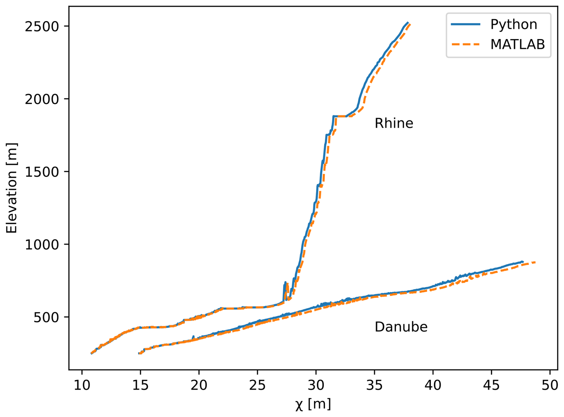
Figure 5 Comparison of χ profiles along the main trunks of the Rhine and Danube computed in both Python and MATLAB using the code in Fig. 2. The χ profiles by Python are shown with the blue solid line and by MATLAB with the dashed orange lines. The discrepancy between the two packages arises from differences in the coordinate transformation applied by Python and MATLAB in Step 2 of Fig. 2. If the DEM is first projected into a coordinate reference system in MATLAB, saved to disk and loaded into Python and then analyzed using Steps 3–6 of Fig. 2, the discrepancy goes away, and the χ profile is identical to the one computed entirely in MATLAB (the dashed orange lines).

3.2 Metamorphic testing

Metamorphic tests identified the problem addressed in pull request #186 when the two FlowObjects created from the same GridObjects in different memory layouts did not appear to be equivalent (Fig. 6a). While libtopotoolbox takes care to scan over 2D arrays in different directions depending on the memory layout of the underlying array, D8 flow routing also scans a neighborhood of each pixel to determine the direction of steepest descent. In case of ties, the first pixel with the steepest gradient encountered during the scan over the neighborhood is chosen. However, the neighborhood was scanned in a clockwise direction in column-major arrays and in a counterclockwise direction in row-major arrays, and ties were therefore encountered in different orders for row- and column-major arrays (Fig. 6c and d). This was fixed in pull request #186 by adding an “order” argument to the flow routing functions in libtopotoolbox. This should be 0 for column-major arrays and 1 for row-major arrays. When it is 1, it flips the direction in which the neighborhood is scanned so that the same pixels are chosen in case of ties (Fig. 6b).

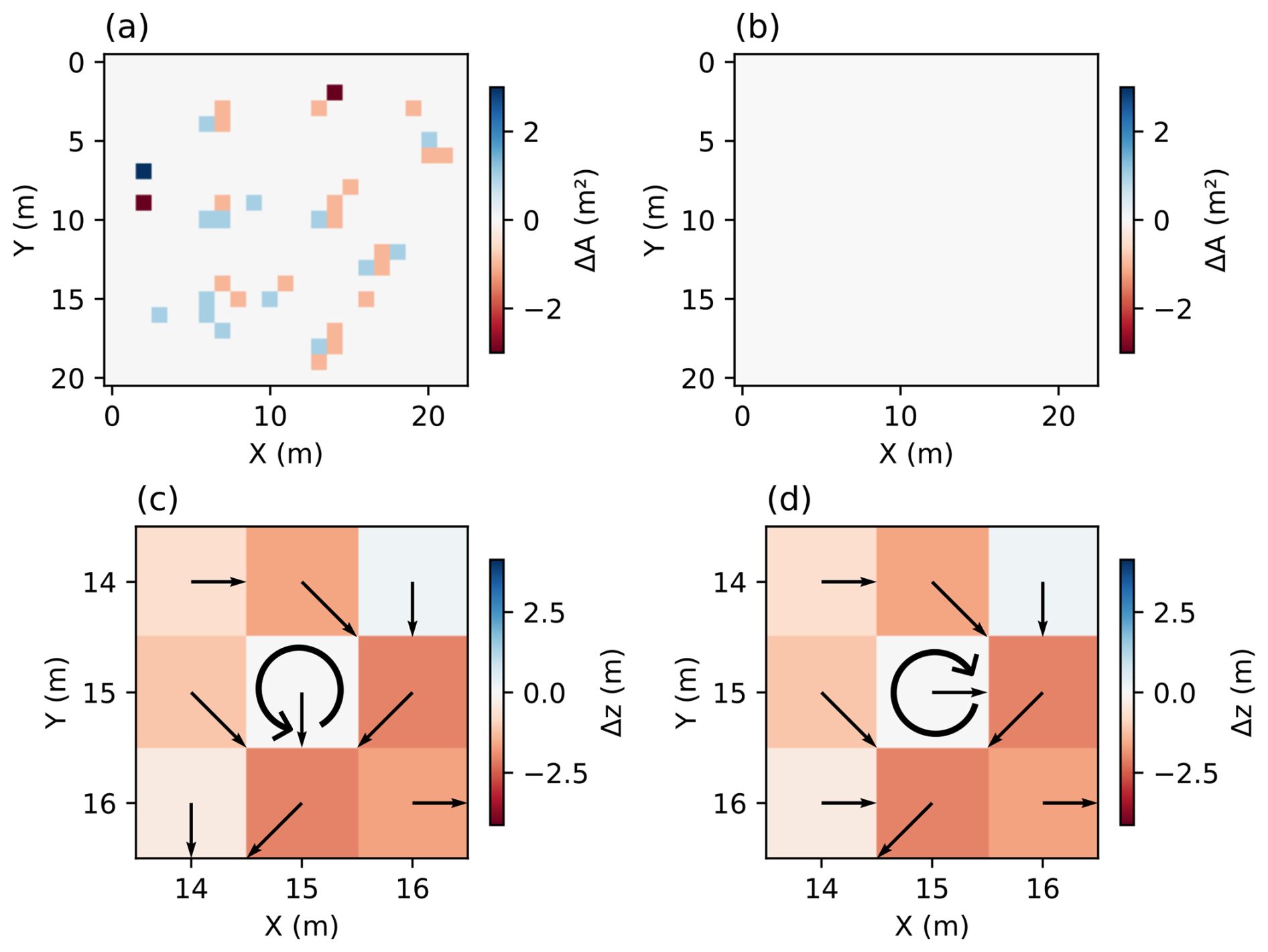
Figure 6 An illustration of metamorphic testing in TopoToolbox 3. (a) The same DEM is generated in row- and column-major layouts and passed to the libtopotoolbox flow routing function “flow_{routing d8 carve}”. The resulting “FlowObjects”, however, are not exactly identical as can be determined from the difference in their corresponding flow accumulation rasters (ΔA). (b) The flow accumulation test after pull request #186 was merged. The difference in the flow accumulation rasters is now zero because each pixel's neighborhood is scanned in the same direction in the row- and column-major layouts. (c) The flow directions obtained prior to the fix from the row-major DEM plotted over the elevation normalized to the value of the center pixel. The south and east neighbors all have the same elevation, and the south neighbor is chosen because the neighborhood scan starts to the south for row-major arrays and proceeds counterclockwise as indicated by the circular arrow. (d) The flow directions obtained prior to the fix from the column-major DEM plotted over the elevation normalized to the value of the center pixel. The east neighbor is chosen because the neighborhood scan starts to the east for column-major arrays and proceeds clockwise as indicated by the circular arrow.

3.3 GraphFlood

The GraphFlood simulation of the Saison watershed (Fig. 7a) returns estimates of flood extent (Fig. 7b) and hydrodynamic parameters under the three precipitation scenarios. The patterns of width and shear stress illustrated by the swaths in Fig. 7c do not systematically covary, suggesting that the combination of the two provides more information than either alone. The variability in shear stress across the swath illustrates the value of 2D hydrodynamics in capturing signals beyond along-profile variations such as those that can be analyzed with the 1D methods provided by TopoToolbox's Stream objects.

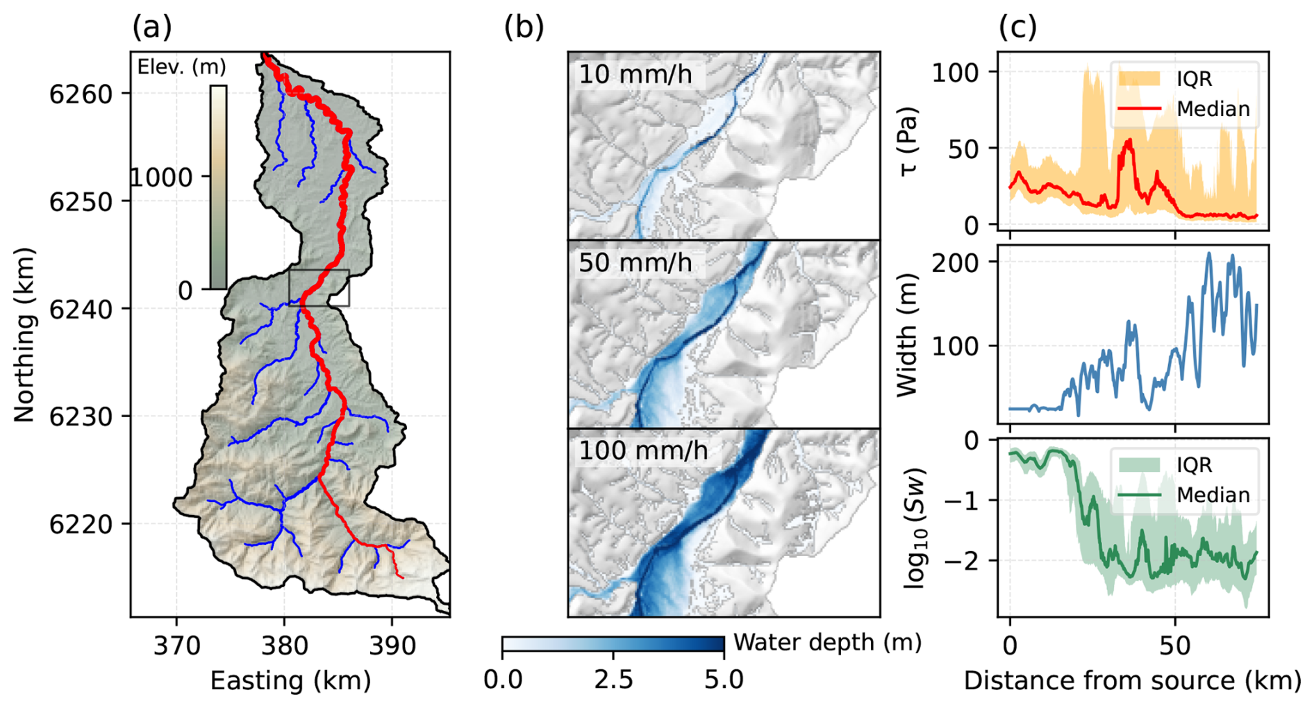
Figure 7 Hydrodynamic analysis of the Saison watershed using GraphFlood and TopoToolbox 3. (a) Topographic map of the area, note the high variability in fluvial relief and valley confinement. (b) Simulated water depth over a portion of the valley floor for three precipitation rates to explore inundation patterns. (c) Hydrodynamic parameters in the vicinity of the main trunk: hydraulic slope (S_w), channel width (W) and fluvial shear stress (τ). The hydraulic slope and fluvial shear stress panels show the median (solid line) and interquartile range (IQR, shaded region) of the respective quantity computed from all pixels within a swath of 500 m on either side of the main trunk. Details of the simulation and analysis can be found in the accompanying Jupyter notebook.

TopoToolbox is now the main outlet for the ongoing development of GraphFlood, combining traditional topographic analysis with physics-based hydrodynamics at the basin scale. The core GraphFlood algorithm is implemented in libtopotoolbox and is exposed in both the Python and MATLAB packages. The Python implementation wraps this implementation in an object-oriented interface (GFObject) to make it easier to configure model runs and manage the input data and results. The GraphFlood methods in either package take Grid objects as input and return them as output so users can load their own data, configure and run the model and then analyze and visualize the results using other TopoToolbox functions. Developing GraphFlood within TopoToolbox allows even a complex numerical model like GraphFlood to be easily distributed to users who can seamlessly integrate it into their workflows.

3.4 Integration with Landlab

Figure 8 shows the simulated elevations and the stream network with knickpoints identified by TopoToolbox at three timesteps of the Landlab simulation: just before the uplift rate is adjusted (Fig. 8a) and at 100 000 years (Fig. 8c) and 200 000 years after the uplift rate adjustment (Fig. 8e). The stream profiles and knickpoints are also visualized in χ plots (Fig. 8b, d, and f). As the balance of erosion against uplift approaches steady state (Fig. 8b), the stream profiles collapse towards one another in χ space. They do not collapse perfectly indicating that a steady state between erosion and uplift has not been fully reached by 2 million years, which is affected by the relatively high hillslope diffusion coefficient used here (0.05 m² yr⁻¹). When the uplift rate is increased (Fig. 8d), knickpoints form, which cluster in χ space as expected, and they migrate upstream at the theoretical celerity of knickpoints in the stream power model (Berlin and Anderson, 2007; Perron and Royden, 2013).

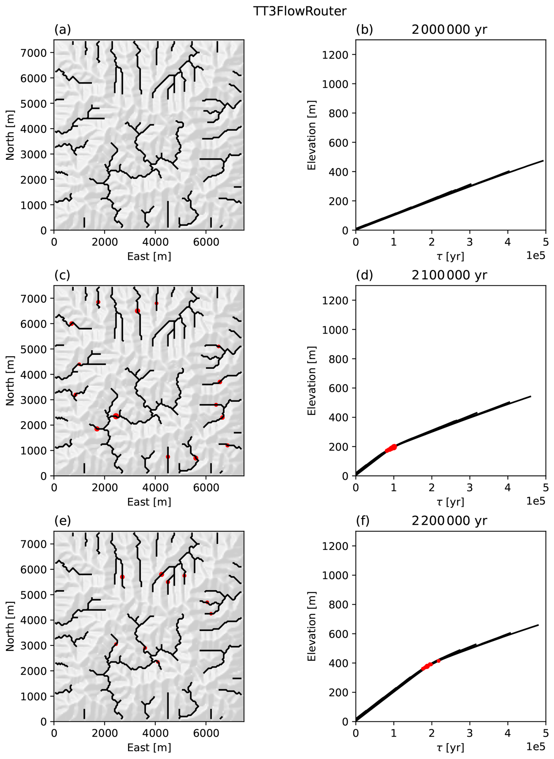
Figure 8 A simulation of knickpoint migration in Landlab using TopoToolbox for flow routing, knickpoint identification and visualization. The figures show the simulation at 3 time steps beginning at (a, b) when the uplift rate is adjusted from 1 to 2 mm yr⁻¹ and showing the stream network and knickpoints after (c, d) 100 000 and (e, f) 200 000 years. Panels (a), (c), (e) show a hillshade topography along with the stream network identified by TopoToolbox (black) and knickpoints (red). Panels (b), (d), (f) show the elevation vs the time scale τ, which is χ normalized by the erodibility coefficient, for the stream network.

The TopoToolbox flow router produces nearly identical results to the Landlab FlowAccumulator with a FlowDirectorD8 and DepressionFinderAndRouter. The differences between the two are due to differences in how each flow router resolves topographic sinks and computes flow directions over flat areas. These differences affect the early stages of the simulation before sinks in the random initial conditions are removed by the combined effects of uplift, erosion and diffusion, but small differences introduced early in the simulation grow into large differences at the end of the simulation. To minimize the impact of these effects on the final results, the random initial conditions are modified using TopoToolbox's imposemin function to carve a channel through the initial conditions with a small minimum slope ($\mathrm{1}\times {\mathrm{10}}^{-\mathrm{5}}$). With minimum imposition on the initial conditions the mean absolute difference between the elevations simulated with the two different flow routers is 0.8 m at the end of the simulation. However, there can be differences in the simulated elevation of individual pixels on the order of 200 m as show in Fig. 9.

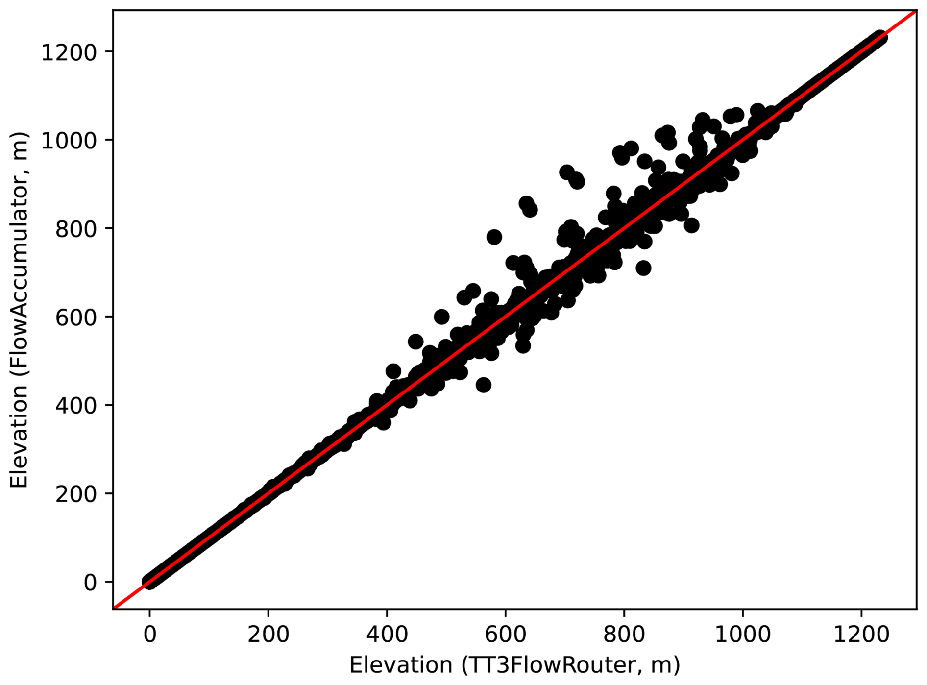
Figure 9 The elevation values of each pixel in the simulation at the end of the simulation computed with the Landlab FlowAccumulator component (vertical axis) and the TT3FlowRouter component (horizontal axis). The red line is the one-to-one line that indicates perfect agreement between the two models.

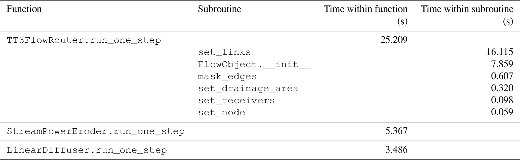
The entire simulation runs in 24.1 s using the TopoToolbox flow router and in 44.7 s using the Landlab FlowAccumulator with a FlowDirectorD8 and the DepressionFinderAndRouter (simulations were run on a Linux workstation with a 2.3 GHz Intel Core i7-11800H processor with 8 cores and 32 GB of RAM). The original example from the Landlab documentation does not use the DepressionFinderAndRouter (Wickert and Gasparini, 2026), but it is included to make better comparisons with pytopotoolbox, which currently always resolves sinks when routing flow. The Landlab simulation is much faster without the DepressionFinderAndRouter (11.5 s). Work is ongoing in TopoToolbox to expose flow routing without sink resolution in pytopotoolbox, which should improve the speed of such simulations because sink resolution is the slowest part of TopoToolbox's flow routing algorithm. However, profiles collected using Python's profile module show (Table 2) that converting TopoToolbox's topologically sorted edge list into the list of links required by Landlab (the set_links subroutine) takes around twice as much time to run as the flow routing itself (FlowObject.__init__).

Table 2 Profile of the Landlab simulation. The outer functions are the update functions called on Landlab components within the main simulation loop. The subroutines called by the TT3FlowRouter are also shown for more detailed comparison. These subroutines are not shown in Fig. 3 for brevity, but they correspond to the commented sections of code within that function.

4 Discussion

In this section, we first examine the FAIR principles for research software and asses how well TopoToolbox 3 follows them. We then discuss the effectiveness of the testing and quality assurance framework. Finally, we examine the modes in which TopoToolbox can be extended by its users and describe the pathways for users to contribute their own software to the TopoToolbox ecosystem.

4.1 FAIR principles

The FAIR Principles for Research Software (Barker et al., 2022) provide a set of best practices for research software development that guided the design of TopoToolbox 3. These principles state that research software should be findable, accessible, interoperable, reusable. The components of TopoToolbox 3 and accompanying metadata are findable through GitHub as well as the Zenodo archive. Zenodo provides a DOI that serves as a persistent identifier for each released version of the software. The software is accessible in source or precompiled forms from GitHub, and the Python package is registered in the Python Package Index, allowing users to install it with Python's standard packaging tools. Zenodo also allows users to download the source code of each repository as well as metadata. TopoToolbox 3 interoperates with other software by exchanging raster data through standard file formats, and it provides methods for exporting flow and stream networks to vector data files that can be interpreted by other software. TopoToolbox 3 also exchanges information directly between higher-level programming languages and libtopotoolbox by representing all necessary data as flat arrays, so they can be accessed through interfaces provided by Numpy and MATLAB. TopoToolbox 3 can be reused, modified and built upon because it is released as free software under the GNU Public License v3.0. Development is tracked in the Git version control system to establish the provenance of all artifacts incorporated into TopoToolbox 3. Packaging, distribution and dependency management are provided by standard mechanisms in each language, allowing users to install and use the package alongside other software.

Each function in TopoToolbox is documented in the source code with descriptions of its arguments and outputs and brief usage examples. This documentation is available to users on the new TopoToolbox website (https://topotoolbox.github.io, last access: 6 November 2026) and through the MATLAB Help Center. The Python and MATLAB packages also come with a guide to Getting Started with TopoToolbox. User-contributed examples are provided as executable Jupyter notebooks and MATLAB Live Scripts through the TopoToolbox gallery (https://topotoolbox.github.io/gallery, last access: 6 November 2026). Supplementing this official documentation is the long-running TopoToolbox blog (https://topotoolbox.wordpress.com, last access: 6 November 2026), which describes many more use cases and workflows.

TopoToolbox is developed openly on GitHub, and contributions to any of the TopoToolbox packages are accepted from the community. The TopoToolbox GitHub organization (https://github.com/TopoToolbox, last access: 6 November 2026) owns the official GitHub repositories for pytopotoolbox, topotoolbox3, libtopotoolbox and others, but any user can fork a TopoToolbox repository, make changes, and contribute them back through a pull request workflow described in the TopoToolbox Contribution Guidelines (Kearney, 2026). Once a contributor makes a pull request, a TopoToolbox maintainer works with them to ensure that the pull request passes the automated test suite, that it successfully addresses any pertinent bug or issue reports, that it comes with sufficient tests and documentation to enable users and other contributors to make use of the code, and that it meets the stylistic guidelines of the repository, which are documented in each repository's contribution guidelines. There is currently no formal process to become a TopoToolbox maintainer who has permission to merge pull requests, and contributors who have made contributions to TopoToolbox repositories and who express a willingness to help new contributors through this process can be given this permission by existing maintainers.

The automated testing and publishing of software and metadata through continuous integration ensures that the FAIR Principles continue to hold as TopoToolbox is modified and extended. The remaining technical challenges facing the sustainability of TopoToolbox lie largely in improving and maintaining interoperability with other software. Passing flow network information to Landlab, for example, requires an expensive indexing operation every time the flow network is updated because TopoToolbox does not maintain within its data structures all of the information required by Landlab' StreamPowerEroder. Standardized representations of flow networks within the Earth surface processes community could make such integrations smoother and less dependent on the internal implementation details of each library.

4.2 Quality assurance and the problem of platform dependence

The testing strategy outlined above serves three major roles in TopoToolbox 3. It characterizes the informally specified behavior of TopoToolbox 2 and ensures that TopoToolbox 3 does not unintentionally change that behavior. It confirms that new implementations of algorithms in libtopotoolbox and the interface between libtopotoolbox and other packages behave as expected and continue to behave that way as changes are made. Finally, it ensures the consistency of behavior across packages, so that an analysis done in Python will produce the same result as the same analysis done in MATLAB.

Testing helps to manage the complexity of the expanding TopoToolbox ecosystem. As TopoToolbox has grown to include new contributors adding code in multiple programming languages, it is increasingly challenging for any single developer to hold the entire system in their head. The tests instead serve as a shared repository of knowledge about the system, and automated testing and continuous integration ensures that the properties described by the tests continue to hold. Contributors can make changes knowing that they will not break other components without warning, and the tests they contribute specify how their components behave as further changes are made. We do not practice strict test-driven development (Beck, 2003) where failing tests are added before implementing any new code. Instead, we let the tests coevolve with the code, enabling more flexible experimentation, especially when it is unclear how code should be tested or what properties need to be preserved. This does require careful code review when changing the tests to ensure that the safeguards provided by the tests continue to operate.

As TopoToolbox 3 has grown beyond MATLAB, we have encountered the problem of maintaining consistency across different computational platforms, the combinations of hardware, operating systems, programming languages, libraries and user code that make up a software application (Bartelheimer et al., 2022). Ideally, the results of an analysis conducted with TopoToolbox 3 would be the same regardless of whether a user conducted the analysis in MATLAB on a Windows PC or in Python on a Mac as the scientific validity of an analysis is undermined if its results depend on the platform used to run it. The χ maps example (Fig. 5) show that, unfortunately, there can be significant differences between the results of analyses implemented on different platforms.

Both the Python and MATLAB versions of TopoToolbox depend on external libraries for some of their functionality. These dependencies can pose a risk to the future stability of both TopoToolbox and to the reproducibility of scientific results generated with TopoToolbox because the libraries may change their behavior. While this risk is clearly visible in the Python package, where its dependencies are open source packages developed by the community, it does also affect the MATLAB package. One of the major updates required to the MATLAB package during the transition to TopoToolbox 3 involved how georeferencing information is maintained in the GRIDobj, FLOWobj and STREAMobj, which was necessitated by changes in MATLAB's Mapping Toolbox.

In thinking about these risks, we can roughly categorize TopoToolbox's external dependencies into two categories: interface dependencies and computational dependencies. Interface dependencies load information into and export information from TopoToolbox. Libraries like rasterio and the Mapping Toolbox read and write data from storage, and visualization libraries like matplotlib are used to communicate the results of analyses. In principle, changes to interface dependencies should not change the results of an analysis, but only the process by which that analysis is obtained. If matplotlib ceased to exist, the plotting functionality of pytopotoolbox would no longer work, but alternative plotting libraries could still be used with the same GridObjects, FlowObjects and StreamObjects as before, or the data could be exported for visualization in another system. Computational dependencies perform components of the topographic analyses. Libraries like Python's numpy and scipy and MATLAB's Image Processing Toolbox are used primarily as computational dependencies. The reprojection functionality of rasterio and the Mapping Toolbox illustrates that libraries that primarily serve as interface dependencies can also be computational dependencies when they manipulate data while loading it. Changes to computational dependencies may change the results of an analysis, and upgrading these dependencies must be handled with care through extensive testing.

TopoToolbox 3 relies on the shared implementation of functions in libtopotoolbox and cross-platform testing, especially snapshot characterization tests and metamorphic testing as demonstrated in the array memory layout example, to minimize the dependency of its results on the underlying platforms. These two strategies guaranteed that the discrepancy in the MATLAB and Python outputs for the χ maps did not originate in the flow routing, flow accumulation or χ transform code, all of which is done in libtopotoolbox and tested across platforms. The only remaining computation in that example is the transformation of the OpenTopography data to a projected coordinate system. Bypassing reprojection by transforming the data in MATLAB and using that saved dataset directly in Python confirms that the discrepancy arises entirely in the functions GRIDobj.project and GridObject.reproject. These are implemented using raster transformation functions from the MATLAB Mapping Toolbox and rasterio, respectively. While we nominally apply the same settings in each case – bilinear resampling to a fixed 90 m resolution – it is clear that either the underlying implementations or the TopoToolbox interfaces to those implementations make additional assumptions that result in different answers.

The discrepancies observed in the Landlab example (Fig. 9) are of a similar nature: both Landlab's FlowAccumulator with FlowDirectorD8 and the TT3FlowRouter implement D8 flow routing, but they make different choices in how they route flow through depressions and over flat regions. These algorithmic differences can add up to large maximum absolute differences in the simulated elevations (over 200 m) even if the mean absolute difference is quite small. However, these results were only obtained by modifying the initial conditions explicitly to minimize the impact of the different sink resolution algorithms, and the discrepancies are much larger when using completely random initial conditions.

TopoToolbox's automated test suites are tools for software development, not scientific investigation. They are verification tests, which check that the software faithfully implements its specifications, not validation tests, which check that the model implemented by the software faithfully represents the real world (Kelly and Sanders, 2008). The automated tests do not replace the essential scientific work of validating the algorithms implemented by TopoToolbox. Because the DEM is only an approximation of the real landscape (Fisher and Tate, 2006; Purinton and Bookhagen, 2017; Schwanghart and Scherler, 2017; Voigtländer et al., 2024), there will always be a limit to how well tests such as those we have illustrated here can validate the assumptions of the algorithms implemented in the software. We instead advocate careful comparison of the outputs of TopoToolbox to independent data sets and to the outputs of other software and models. Because TopoToolbox 3 can be integrated more tightly with other software, it is now much easier to make these comparisons as illustrated in the Landlab example above. Validating the theoretical behavior of knickpoint migration and comparing the output of the Landlab FlowAccumulator with that of the TopoToolbox TT3FlowRouter were both essential for correctly implementing the TT3FlowRouter. At the same time, the test cases contributed to TopoToolbox do not need to demonstrate scientific validity. An algorithm intended for large-scale DEM analysis might require large datasets and complicated analyses to validate it properly, tests which are hard to develop and costly to run. Property-based tests with small, randomly generated DEMs can verify that the implementation in TopoToolbox works as expected with a lower computational expense and a smaller software development and maintenance burden.

4.3 Extensibility

One of the strengths of TopoToolbox is providing a foundation upon which users can build their own tools for more specialized analyses. The architecture of TopoToolbox 3 opens new paths to extend the software. TopoToolbox 3 can still be used by exchanging raster or vector data files between it and other tools. Users who need only a small portion of the functionality of TopoToolbox, who would prefer to do the majority of their analysis in another tool such as a GIS, or who do not need tight, interactive coupling between TopoToolbox and their other tools may find this approach the easiest to get started with. In this case, the new Python interface can be valuable for this kind of analysis even if users are not relying on more sophisticated integration between TopoToolbox and other Python-based software.

The GraphFlood and Landlab applications described above demonstrate two other ways that TopoToolbox 3 can be extended. GraphFlood is implemented in libtopotoolbox, and interfaces in both the Python and MATLAB packages expose this functionality to users of either programming language. Implementing an extension in libtopotoolbox allows it to be used from both MATLAB and Python, but it does require implementing the tool in C, subject to constraints on external dependencies, dynamic memory management and data formats imposed by the design of libtopotoolbox.

Alternatively, extensions can be built in high-level languages using the core TopoToolbox functions alongside external dependencies. The Landlab integration, for example, is implemented purely in Python. It uses TopoToolbox functions to perform the necessary analyses and provides interface functions that convert data between the formats expected by Landlab and TopoToolbox as well as a class implementing the Landlab component interface. Packages have also been developed in this style in MATLAB, including ttminvoellmy, an interface to the MinVoellmy avalanche model (Hergarten, 2024a, b), and BankfullMapper, a toolkit for semi-automatic bankfull geometry extraction and discharge estimation (Delchiaro et al., 2025). Software developed in this way can use the standard dependency resolution mechanisms of their programming languages to depend on TopoToolbox. Users can maintain such extensions independently of the TopoToolbox organization if they desire. However, the TopoToolbox organization and its online documentation and discussion forums can publicize such extensions and illustrate how they can be used.

5 Conclusions

TopoToolbox has provided a platform for research in the computational geosciences for the past 15 years. The changes introduced in TopoToolbox 3 facilitate a sustainable development process that ensures the platform will continue to meet the needs of the community for the decade to come. The new architecture, based around the portable core library, libtopotoolbox, and its interfaces in several high-level languages, makes it easier to combine TopoToolbox with other software, such as the Landlab framework, to create interactive data visualization and modeling systems and to disseminate new research software like GraphFlood. It also offers the potential to combine TopoToolbox with libraries for high-performance computing and machine learning to open new frontiers in computational geomorphology. Quality assurance practices including an automated test suite and continuous integration make it possible to change individual components with confidence that the entire system will function as expected.

Development of TopoToolbox is ongoing, and we encourage the community to participate in this process. Collaboration occurs through the GitHub issue trackers for each package, which list outstanding tasks and through which contributors can discuss new features and changes to existing ones. As of this writing, development efforts focus on achieving complete feature parity between the Python and MATLAB packages, building out the R and QGIS integrations, prototyping high-performance implementations of TopoToolbox analyses, and expanding and improving the documentation. Counterparts of the DIVIDEobj and SWATHobj, further elaboration of the point pattern on stream networks object, PPS, and more sophisticated and user-friendly visualization tools are excellent opportunities to contribute to the Python package. The R package and integration for QGIS are in early stages of development, and we welcome users of R or QGIS to help guide the design of those tools. Implementations of algorithms that take advantage of hardware acceleration and parallel computing can enable analysis at larger scales, higher resolutions and greater physical fidelity. Documentation and examples of analyses that can be added to the TopoToolbox Gallery are particularly impactful contributions from the community as they showcase the broad range of applications of TopoToolbox. Above all, TopoToolbox aims to establish a community of practice in quantitative geomorphology: user involvement in the future development of TopoToolbox is crucial to ensure that TopoToolbox evolves to solve the problems that users encounter in their study of the Earth's surface.