Seismic signature of turbulence during the 2017 Oroville Dam spillway erosion crisis

Knowing the location of large-scale turbulent eddies during catastrophic flooding events improves predictions of erosive scour. The erosion damage to the Oroville Dam flood control spillway in early 2017 is an example of the erosive power of turbulent flow. During this event, a defect in the simple concrete channel quickly eroded into a 47 m deep chasm. Erosion by turbulent flow is difficult to evaluate in real time, but near-channel seismic monitoring provides a tool to evaluate flow dynamics from a safe distance. Previous studies have had limited ability to identify source location or the type of surface wave (i.e., Love or Rayleigh wave) excited by different river processes. Here we use a single three-component seismometer method (frequency-dependent polarization analysis) to characterize the dominant seismic source location and seismic surface waves produced by the Oroville Dam flood control spillway, using the abrupt change in spillway geometry as a natural experiment. We find that the scaling exponent between seismic power and release discharge is greater following damage to the spillway, suggesting additional sources of turbulent energy dissipation excite more seismic energy. The mean azimuth in the 5–10 Hz frequency band was used to resolve the location of spillway damage. Observed polarization attributes deviate from those expected for a Rayleigh wave, though numerical modeling indicates these deviations may be explained by propagation up the uneven hillside topography. Our results suggest frequency-dependent polarization analysis is a promising approach for locating areas of increased flow turbulence. This method could be applied to other erosion problems near engineered structures as well as to understanding energy dissipation, erosion, and channel morphology development in natural rivers, particularly at high discharges.

1 Introduction

Dam spillways are typically designed with features that generate controlled turbulent eddies, such as steps or changes in slope. These eddies entrain air into the flow, increase energy dissipation, and lower the mean flow velocity (Hunt and Kadavy, 2010a, b). Some of this dissipated energy is transferred as lift and drag forces on the bottom of the spillway channel. If a defect in the spillway channel is present, increased turbulence and associated forces can quickly enlarge the defect, eroding the spillway and underlying embankment (USBR, 2014). In some cases, erosion propagates headwards, undermining the structural integrity of the dam (USBR, 2014). Structural elements and routine maintenance are designed to minimize these channel defects, however, they can develop quickly during extreme flows. Therefore, real-time monitoring of spillway turbulence during times of high release could provide early warning of the onset of erosion. Although turbulence can be characterized with photographic images or measurements of velocity time series with submerged or overhead instrumentation, these procedures may be impractical on large structures or during catastrophic events. Seismic monitoring may provide a way to continuously evaluate turbulent intensity and associated erosion from safely outside channels or hydraulic structures.

Seismic waves have previously been used to characterize the geotechnical suitability of earthen dams and internal dam seepage using passive seismic interferometry (e.g., Planès et al., 2016), but have not been used to characterize open-channel turbulence in dam spillways. Because turbulence affects erosional processes in both hydraulic structures and natural rivers, techniques from seismic river monitoring (fluvial-seismic) literature provide guidance. In the past decade, many authors have used near-channel seismometers to monitor rivers during monsoons (e.g., Burtin et al., 2008), natural floods (e.g., Govi et al., 1993; Hsu et al., 2011; Burtin et al., 2011; Roth et al., 2016), and controlled floods (Schmandt et al., 2013, 2017). In many of these studies, the authors seek to separate the various sources of seismic energy, including precipitation, bedload transport, and flow turbulence (e.g., Roth et al., 2016). Bedload transport is traditionally difficult to monitor, therefore, research has been focused on isolating this source. Characterizing turbulence in rivers has been given less consideration in the fluvial-seismic literature, even though macroturbulent eddies place important controls on channel erosion (Franca and Brocchini, 2015) and may be important in spillway erosion. A forward mechanistic model by Gimbert et al. (2014) estimates the power spectral density of seismic energy produced by turbulently flowing water in a simple rectangular channel, in principle making it possible to use seismic data to invert for river depth and bed shear stress. This model, however, is based on assumptions of spatially uniform turbulence created by bed grain size; it ignores other sources of turbulence common in natural rivers and in engineered structures such as deviations from spatial uniformity. Recent work (Roth et al., 2017) suggests that hysteresis between seismic power and discharge may also result from riverbed particle rearrangement, which leads to different turbulent characteristics within the flow. This fluvial seismic body of work suggests seismic monitoring may be able to resolve hydraulic changes in a dam spillway setting.

A near-spillway seismometer records seismic energy excited by a number of sources from different directions across a range of frequencies. These potential sources include primary and secondary microseisms, anthropogenic noise, wind, rain, earthquakes, and nearby rivers. Without a way to differentiate among these sources by direction and frequency, interpreting seismic observations will be limited. This challenge was highlighted by Roth et al. (2016, 2017), who indicated that the turbulent signal from a waterfall downstream of their study river reach may have dominated the observed low-frequency signals. Previous studies have attempted to locate the source of fluvial seismic energy by using arrays of seismometers, primarily by observing the variability in seismic amplitudes around the river section of interest (Burtin et al., 2011, and Schmandt et al., 2017). A study by Burtin et al. (2010) developed noise correlation function envelopes to identify segments of the Trisuli River that generated the most seismic energy at a given frequency. The greatest coherence between seismometer pairs (and inferred greatest seismic energy production) was located along river segments with the steepest river slopes and highest estimated incision rates. This approach is a promising one, although it requires an extensive array of seismometers. A single-seismometer method for distinguishing various sources of seismic energy at different frequencies is more likely to be implemented in monitoring hydraulic structures and may be advantageous for fluvial seismic studies.

Discerning among seismic sources using a single station requires an evaluation of the three-dimensional ground motion recorded by a three-component seismometer. In traditional earthquake seismology, these motions indicate the arrival of body waves (P and S) and surface waves (Rayleigh and Love). For continuous ambient seismic sources such as turbulence, the phase relationships between the signals in each component can provide information on the wave type and its propagation direction. Several researchers have suggested that turbulence may excite Rayleigh surface waves whereas sliding and rolling bedload transport may excite Love surface waves, although these authors relied on comparing the seismic power of the three components rather than analyzing phase relationships among the components (Schmandt et al., 2013; Barrière et al., 2015; Roth et al., 2016). While recent forward models to estimate the power spectral density of seismic energy produced by moving bedload and turbulently flowing water can accommodate the excitation of various seismic waves, their applications to date assume that only Rayleigh waves are excited (Tsai et al., 2012; Gimbert et al., 2014). This assumption has not been quantitatively tested. Identifying the surface wave type excited by turbulent sources will help to identify the dominant mechanisms generating seismic waves in spillways and natural channels.

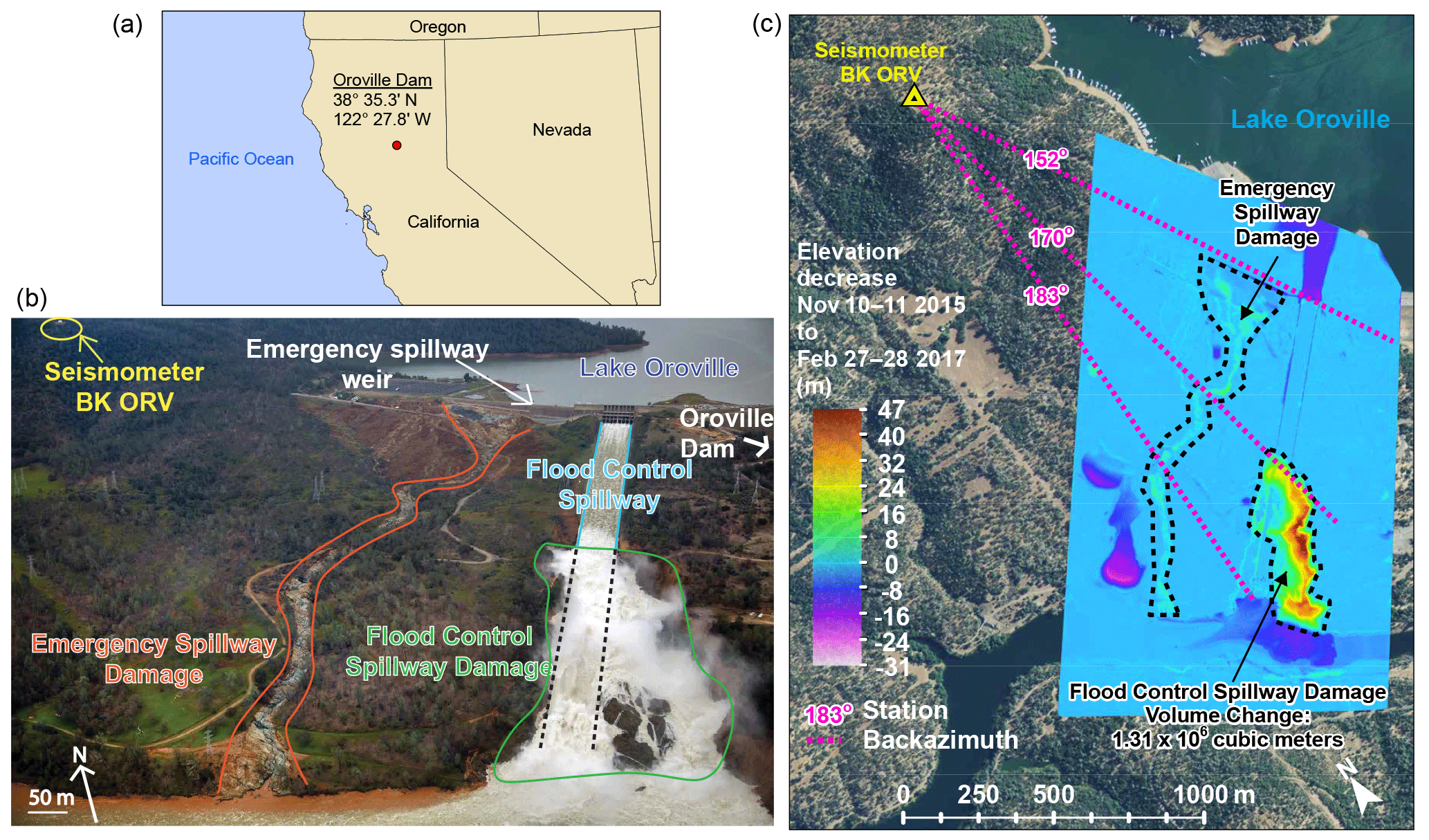
Figure 1 (a) Location of the Oroville Dam in northern California. (b) The damage created along the flood control and emergency spillways of Oroville Dam in February and March, 2017. The seismometer used in this study is located approximately 2 km from the spillway. Photo credit: Dan Kolke, Department of Water Resources. Image taken on 15 February 2017. Estimated discharge during photograph is 2800 m³ s⁻¹. (c) A digital elevation model created from lidar points provided by the California Department of Water Resources. The elevation difference from a November 2015 elevation survey and a late February 2017 survey shows that the crisis incised a chasm up to 47 m deep. The volume of the main chasm is 13 × 10⁶ m³. The incision resulting from the use of the emergency spillway is less than 20 m deep. The back-azimuth (clockwise from north) in degrees is displayed for the top of the flood control spillway, the top of the chasm, and the bottom of the flood control spillway. The seismometer is at an average 13^∘ slope above the base of the flood control spillway and an average 8^∘ slope above the top of the flood control spillway.

In this study we employ a single-seismometer method to observe variations in turbulence intensity and location within a dam spillway. Our goals are to (1) evaluate the scaling exponent between seismic power and discharge for different turbulence and channel roughness conditions, (2) determine if a single-seismometer source location technique can be used to resolve changes in the location of flow turbulence in a spillway channel, and (3) evaluate the surface wave type excited by spillway turbulence and erosion. The study site is the flood control spillway of the Oroville Dam, California, United States. Seismic and discharge data collected during the erosional event that damaged the flood control spillway in February and March 2017 provide a natural experiment for this study, during which a simple and straight channel was abruptly eroded into a complex one.

2 Oroville Dam crisis

The Oroville Dam, located 100 km north of Sacramento, CA in the Sierra Nevada foothills, is the tallest dam in the United States (Fig. 1a). The dam spans the Feather River and provides hydroelectric power, flood control, and water storage for irrigation. Completed in 1968, the dam is constructed on Mesozoic volcanic rocks contained in the Smartville Complex (Saucedo and Wagner, 1992). The dam is built adjacent to the Long Ravine Fault; therefore, a permanent seismic station was placed approximately 2 km from the dam site in 1963 to monitor possible reservoir-induced earthquakes (Lahr et al., 1976). Several studies have linked the unusually large drawdown and refilling of the reservoir in 1974–1975 to a 5.7 magnitude earthquake on 1 August 1975 located 12 km south of the reservoir (Beck, 1976; Lahr et al., 1976). In 1992, the Berkeley Seismological Laboratory installed a Streckeisen STS-1 broadband three-component seismometer at station BK ORV (BDSN, 2014). We are not aware of any studies that have investigated ground motion generated by the flood control spillway.

At approximately 09:00 PST on 7 February 2017, during a controlled dam release of approximately 1400 m³ s⁻¹, a section of the concrete flood control spillway failed, leaving a defect in the spillway. A subsequent preliminary root cause analysis identified construction and maintenance flaws as the source of this initial defect (Bea, 2017; ODSIIFT, 2017a, b). Ongoing heavy rainfall and runoff from the upstream watershed filled the reservoir to near capacity. Reservoir managers increased the discharge through the damaged spillway in a series of tests and ultimately raised the discharge to over 1500 m³ s⁻¹. This discharge and associated high flow velocities resulted in turbulent scour around the defect, rapidly eroding the underlying embankment and incising a gully that bypassed the concrete spillway channel. Dam managers then limited the flood control spillway discharge to below 1800 m³ s⁻¹ (California Department of Water Resources, 2017a). High incoming discharge from the Feather River raised the reservoir level to capacity, which activated an emergency spillway weir for the first time in the dam's 48-year history.

Figure 2 Discharge and inflow at Oroville Dam in early 2017, as reported by the California Department of Water Resources (CA DWR; California Department of Water Resources, 2017d). The five time intervals of constant discharge in early 2017 used in this study are highlighted and labeled. The “Pre-chasm” and “Post-chasm” time intervals have approximately equal discharge, but very different channel geometries. Data gaps in discharge and inflow data are linearly interpolated in this figure. The inflows reported are from the Feather River to Lake Oroville. The discharge displayed for the emergency spillway weir is the maximum reported by CA DWR media updates, as no quantified measurements have been published for this data.

Discharges up to 360 m³ s⁻¹ flowed over the emergency spillway weir beginning at 08:00 PST on 11 February while managers released approximately 1500 m³ s⁻¹ through the primary flood control spillway. Within 32 h, rapid erosion at the base of the emergency spillway weir threatened to compromise its stability, triggering concerns of catastrophic failure. Managers increased the discharge through the previously damaged flood control spillway to 3000 m³ s⁻¹ and evacuated 180 000 people from the downstream city of Oroville, California. Elevated flood control spillway discharges lowered the reservoir level and stopped discharge through the emergency spillway weir on 12 February, 38 h after activation. Elevated discharges continued through the damaged flood control spillway through the end of March, causing tens of meters of vertical incision into the weathered, sheared bedrock underlying the spillway (Bea, 2017). Figure 1b and c show the position of the seismometer and the erosion incurred during the event. The seismometer is 1.4 km from the top of the flood control spillway channel and 1.9 km from the bottom of the channel. Using lidar data collected in 2015 and on 23 March 2017, we compute that 1.3 × 10⁶ m³ of material were removed from the flood control spillway damage area during the crisis, resulting in a vertical incision into the hillside of up to 47 m (Fig. 1c; see Supplement) (Maggie Macias, California Department of Water Resources, personal communication, 2017).

3 Methods

3.1 Data collection and approach

In this study, we evaluate seismic signals detected during the Oroville Dam erosion crisis at broadband seismometer BK ORV, operated by the Berkeley Digital Seismological Network (BDSN, 2014). We divide the crisis period into five time intervals of constant discharge, each of which is longer than 15 h in duration (Fig. 2). During each of these discharge intervals, channel geometry and discharge remain similar, allowing us to document the differences across intervals in the spillway-generated seismic signal. The five time intervals of interest are as follows:

1. “Pre-chasm” interval: 18 h of ∼ 1400 m³ s⁻¹ routine flood control spillway release before the initial spillway damage on 7 February,

2. “Emergency discharge” interval: 38 h interval when the emergency spillway weir was active and ∼ 1500 m³ s⁻¹ were released through the flood control spillway

3. “High discharge” interval: 78 h interval when ∼ 3000 m³ s⁻¹ were released through the damaged flood control spillway,

4. “Post-chasm” interval: 87 h interval of ∼ 1400 m³ s⁻¹ discharge through the damaged flood control spillway, and

5. “Zero outflow” interval: 93 h interval of zero discharge through the flood control spillway, which serves as a control interval.

To encompass the erosion crisis period, we compiled seismic data and spillway discharge data from 1 January to 1 April 2017. For comparison to the erosion crisis, we also compiled seismic data and spillway discharge for the second and third highest release periods during which continuous discharge and seismic data are available. These intervals are from 25 February to 18 March 2006 and 1 March to 1 June 2011. The seismic and discharge data for these intervals were processed identically to the 2017 data. The Northern California Earthquake Data Center is the source of the seismic data for this study and instrument response was causally removed (Haney et al., 2012). The California Department of Water Resources' California Data Exchange Center is the source of all discharge data reported in this study (California Department of Water Resources, 2017d).

3.2 Frequency dependent polarization analysis

We expect that contributions to spillway-generated seismic energy will produce energy across a range of frequencies, analogous to observations in natural channels (Gimbert et al., 2014). Energy sources in different frequency bands may also excite a variety of seismic wave types, which result in different ground particle motions and seismic amplitudes. We extract particle motion polarization attributes at each frequency by applying frequency dependent polarization analysis (FDPA) to the single-station three-component data (Park et al., 1987). The approach in this study is similar to ambient noise analysis applied to seismometer networks, in which the particle motion from ambient noise is characterized (e.g., McNamara and Buland, 2004; Koper and Hawley 2010; Koper and Burlacu, 2015). Following Koper and Hawley (2010), for each component (u_x, u_y, u_z), an hour of record (as ground velocity) is selected and divided into 19 sub-windows that each overlap 50 %. Each sub-window is tapered with a Hanning window, converted to ground acceleration, and the Fourier transform is computed. At each frequency considered (up to the half the sampling frequency), the Fourier coefficients from each of three components are arranged into a 3 × 19 matrix, from which the 3 × 3 cross-spectral covariance matrix is estimated. The eigenvector corresponding to the largest eigenvalue of each 3 × 3 matrix describes the particle motion ellipsoid within the hour of observation at each frequency (Park et al., 1987). Henceforth, we refer to this as the dominant eigenvector. The complex-valued coefficients of this dominant eigenvector describe a particle motion ellipsoid at each frequency, whose properties are analyzed in this paper. The time averaging inherent to this methodology minimizes the influence of transient seismic sources such as earthquakes or intermittent anthropogenic noise. The application of FDPA is useful for identifying polarization characteristics at a range of frequencies, yet for weakly polarized seismic energy the polarization attributes are highly variable with time. Therefore, it is more meaningful to analyze the probability distributions of polarization attributes in time intervals of strong seismic polarization (Koper and Hawley, 2010).

We compute the polarization attributes used in this paper from the complex components of the dominant eigenvector, Z [z₁, z₂, z₃] (Fig. 3). For the benefit of the reader, we briefly summarize their computation below and refer the reader to Park et al. (1987) for additional discussion. Each complex component of Z can be thought of as describing the particle motion at a particular frequency in each of the three orthogonal directions. The azimuth (Θ_H) of the ellipsoid, measured clockwise from north, is determined by calculating the angle defined by the horizontal components of Z on the real plane:

$$\begin{array}{}\text{(1)}& {\mathrm{\Theta }}_{\mathrm{H}}={\displaystyle \frac{\mathit{\pi }}{\mathrm{2}}}-{\tan }^{-\mathrm{1}}\left[{\displaystyle \frac{\mathit{\text{Re}}\left(z_{\mathrm{3}}{e}^{i{\mathit{\theta }}_{\mathrm{h}}}\right)}{\mathit{\text{Re}}\left(z_{\mathrm{2}}{e}^{i{\mathit{\theta }}_{\mathrm{h}}}\right)}}\right],\end{array}$$

where θ_h is the phase angle at which the horizontal acceleration is maximized:

$$\begin{array}{}\text{(2)}& {\mathit{\theta }}_{\mathrm{h}}=-{\displaystyle \frac{\mathrm{1}}{\mathrm{2}}}\arg \left(z_{\mathrm{2}}^{\mathrm{2}}+z_{\mathrm{3}}^{\mathrm{2}}\right)+{\displaystyle \frac{l\mathit{\pi }}{\mathrm{2}}},\end{array}$$

where l corresponds to the smallest non-negative integer that maximizes the expression

$$\begin{array}{}\text{(3)}& {\left|z_{\mathrm{2}}\right|}^{\mathrm{2}}{\cos }^{\mathrm{2}}({\mathit{\theta }}_{\mathrm{h}}+\arg \left(z_{\mathrm{2}}\right))+{\left|z_{\mathrm{3}}\right|}^{\mathrm{2}}{\cos }^{\mathrm{2}}({\mathit{\theta }}_{\mathrm{h}}+\arg \left(z_{\mathrm{3}}\right))\end{array}$$

The range of Θ_H is restricted such that 0^∘ < Θ_H ≤ 180^∘ if $\mathit{\text{Re}}\left(z_{\mathrm{1}}{z}_{\mathrm{3}}^{\ast }\right)<\mathrm{0}$ and 180^∘ < Θ_H ≤ 360^∘ if $\mathit{\text{Re}}\left(z_{\mathrm{1}}{z}_{\mathrm{3}}^{\ast }\right)\ge \mathrm{0}$.

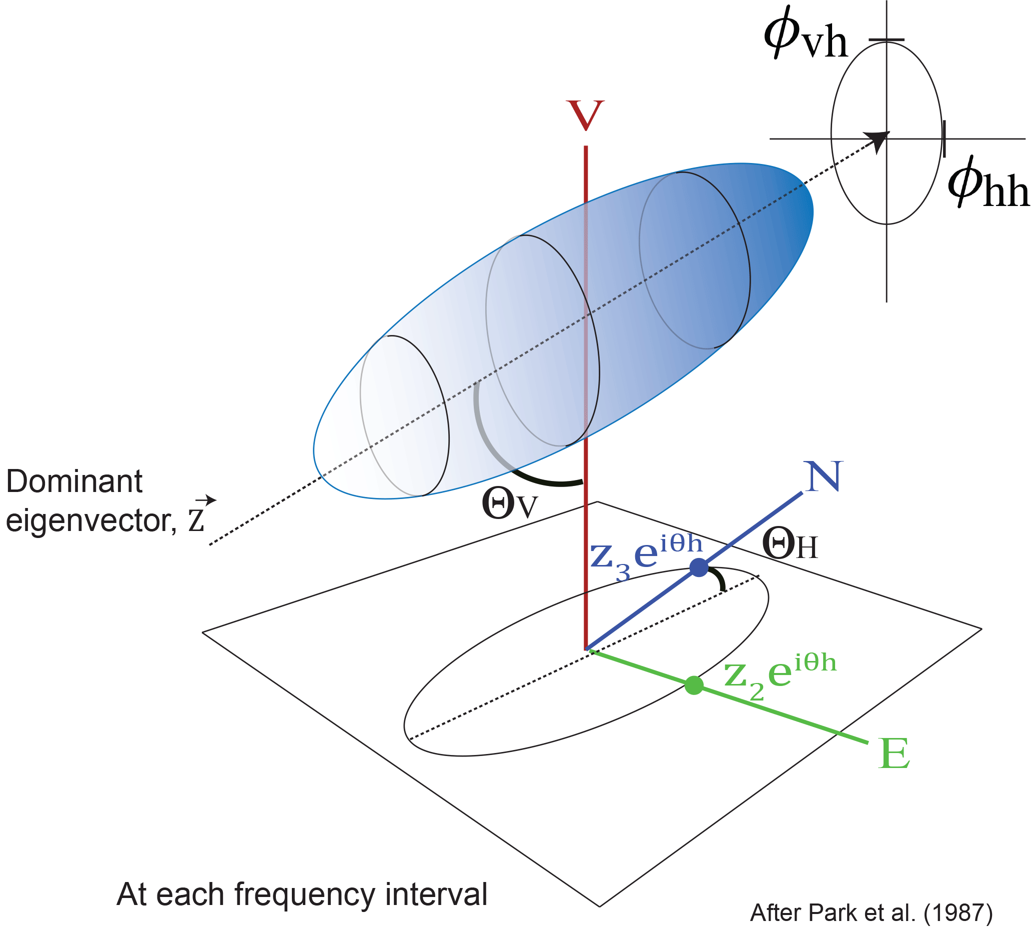
Figure 3 Diagram of particle motion defined by the dominant eigenvector. The particle motion at each frequency is analyzed by considering the dominant eigenvector of the spectral covariance matrix; the complex-valued components of this eigenvector can be visualized as describing a particle motion in an ellipsoid (Park et al., 1987). The orientation of the eigenvector and the phase relationships between the components of the eigenvector yield the polarization attributes.

Analogously, the angle of incidence (Θ_V), measured from the vertical, is computed from the major axis of the particle motion ellipsoid by finding the angle on the real plane defined by the vertical component, z₁, and the total horizontal acceleration, z_H:

$$\begin{array}{}\text{(4)}& {\mathrm{\Theta }}_{\mathrm{V}}={\displaystyle \frac{\mathit{\pi }}{\mathrm{2}}}-{\tan }^{-\mathrm{1}}\left[\left|{\displaystyle \frac{\mathit{\text{Re}}\left(z_{\mathrm{1}}{e}^{i{\mathit{\theta }}_{\mathrm{v}}}\right)}{\mathit{\text{Re}}\left(z_{\mathrm{H}}{e}^{i{\mathit{\theta }}_{\mathrm{v}}}\right)}}\right|\right],\end{array}$$

where

$$\begin{array}{}\text{(5)}& z_{\mathrm{H}}=\sqrt{z_{\mathrm{2}}^{\mathrm{2}}+z_{\mathrm{3}}^{\mathrm{2}}}\end{array}$$

and θ_v is the phase angle at which total acceleration is maximized as follows:

$$\begin{array}{}\text{(6)}& {\mathit{\theta }}_{\mathrm{v}}=-{\displaystyle \frac{\mathrm{1}}{\mathrm{2}}}\arg \left(z_{\mathrm{1}}^{\mathrm{2}}+z_{\mathrm{2}}^{\mathrm{2}}+z_{\mathrm{3}}^{\mathrm{2}}\right)+{\displaystyle \frac{m\mathit{\pi }}{\mathrm{2}}}.\end{array}$$

m, corresponds to the smallest non-negative integer that maximizes the expression:

$$\begin{array}{ll}{\displaystyle }& {\displaystyle }{\left|z_{\mathrm{1}}\right|}^{\mathrm{2}}{\cos }^{\mathrm{2}}({\mathit{\theta }}_{\mathrm{v}}+\arg \left(z_{\mathrm{1}}\right))+{\left|z_{\mathrm{2}}\right|}^{\mathrm{2}}{\cos }^{\mathrm{2}}({\mathit{\theta }}_{\mathrm{v}}+\arg \left(z_{\mathrm{2}}\right))\\ \text{(7)}& {\displaystyle }& {\displaystyle }+{\left|z_{\mathrm{3}}\right|}^{\mathrm{2}}{\cos }^{\mathrm{2}}\left({\mathit{\theta }}_v+\arg \left(z_{\mathrm{3}}\right)\right)\end{array}$$

If $\mathit{\text{Im}}\left(\sqrt{z_{\mathrm{2}}^{\mathrm{2}}+z_{\mathrm{3}}^{\mathrm{2}}}\right)$ < 0^∘, the sign is reversed to restrict Θ_V such that 0^∘ < Θ_V ≤ 90^∘.

We consider two additional angles to describe the particle motion. First, the phase angle difference between the two horizontal components z₂ and z₃ (ϕ_hh) of the primary eigenvector, restricted to within −180 and 180^∘; and second, the vertical–horizontal phase angle difference (ϕ_vh), computed from the phase angle difference between θ_h (Eq. 2) and z₁, restricted to lie between −90 and 90^∘. Following Koper and Hawley (2010), we also compute the degree of polarization (β²) defined by Samson (1983), which is zero when the three component eigenvalues are equal, and is one when the data are described by a single non-zero eigenvalue, such as for a single propagating seismic wave. We emphasize that FDPA methods characterize the dominant seismic source rather than describing the particle motion associated with all sources of seismic energy.

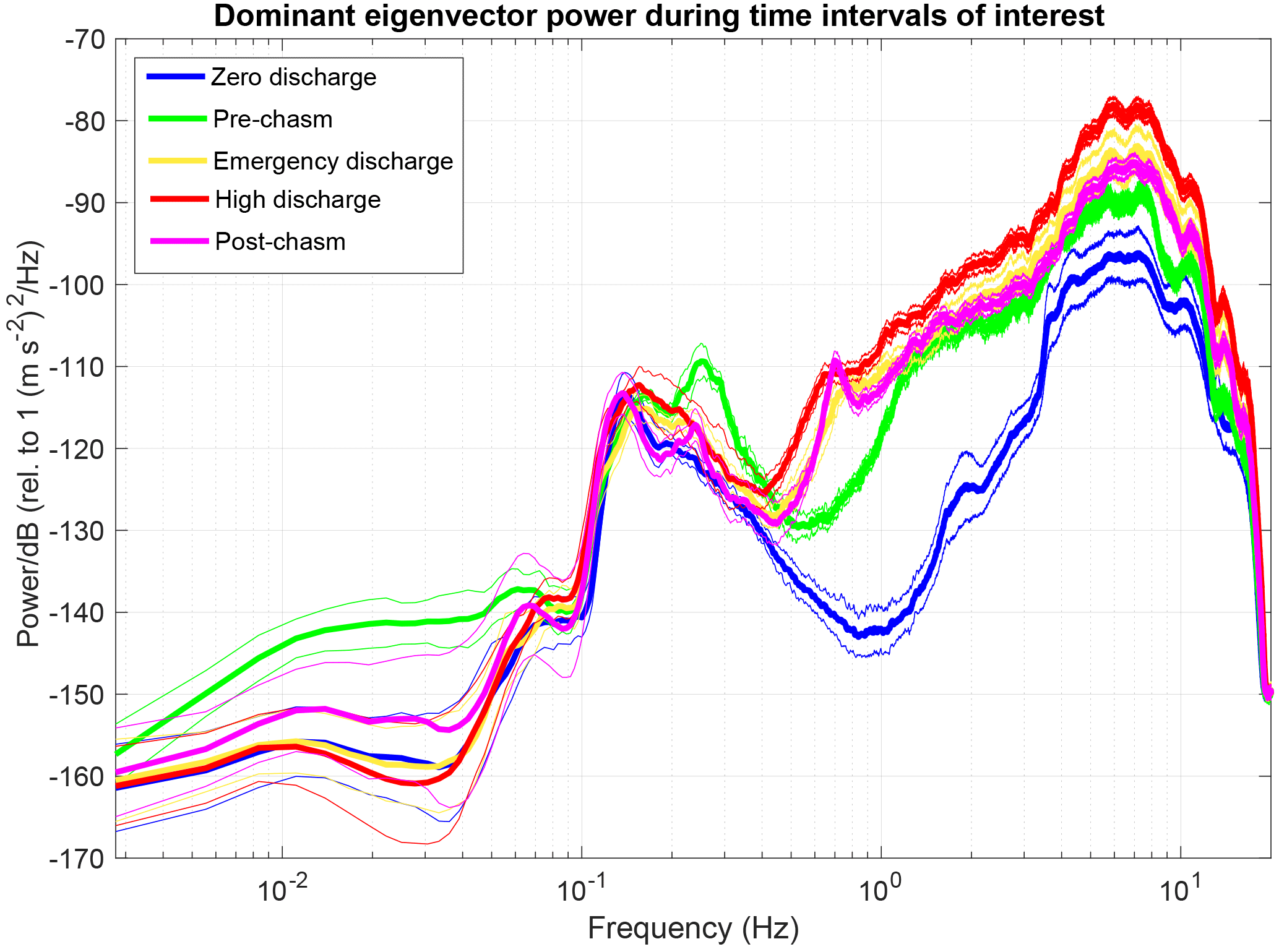
Figure 4 Power spectral density observed for each of the five studied intervals, shown with one standard deviation error bars. There is a significant increase (up to 30 dB) in the average power of the dominant eigenvector during the four time intervals with discharge, particularly between 0.5 and 12 Hz. The power during three time intervals following spillway damage exceeds the “Pre-chasm” at frequencies above 0.5 Hz.

4 Results

In the following analysis, we present the polarization attributes in one hour intervals aligned with the hourly discharge data and assume each hour has a consistent seismic character. We then evaluate the variability of all of the hourly polarization attributes within each constant discharge time interval and throughout the dam erosion crisis.

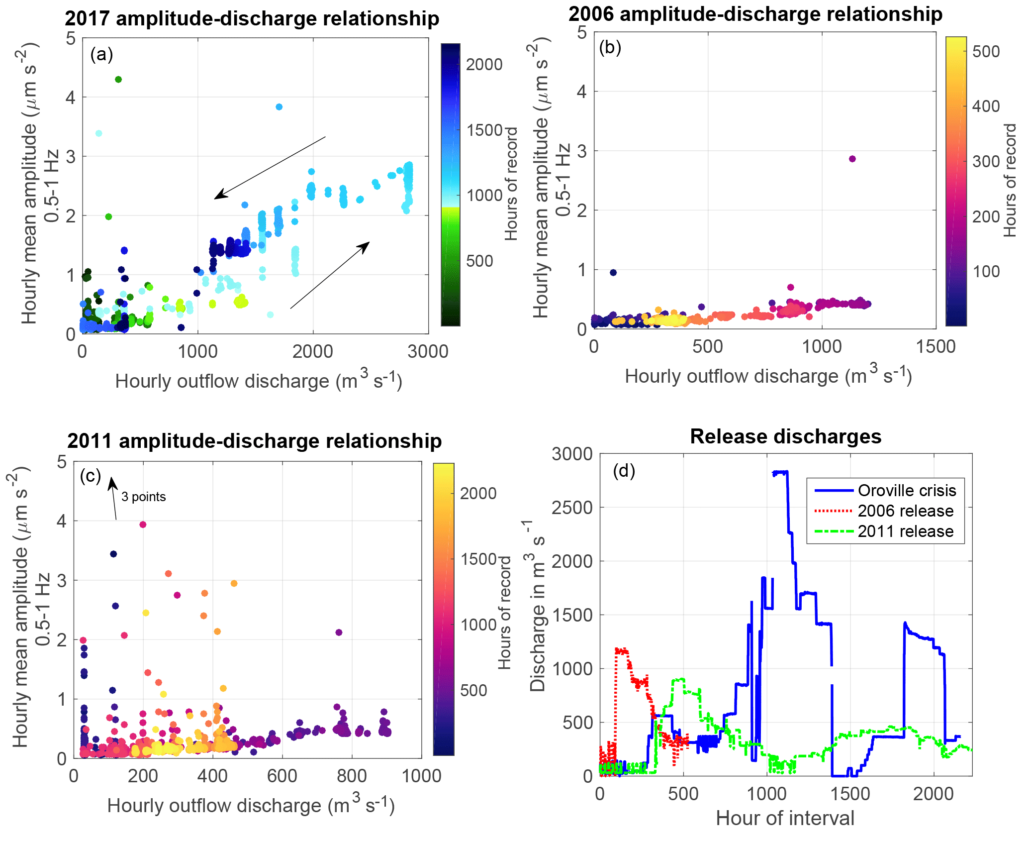
Figure 5 The plot of mean hourly amplitude of the dominant eigenvector in the 0.5–1 Hz frequency band vs. hourly discharge shows that the two correlate strongly. The abrupt change in the color bar coincides with the timing of the Oroville Dam crisis, and allows two distinct regimes to be identified. Seismic amplitudes are greater by ∼ 0.5 µm s⁻² after the uncontrolled channel erosion begins on 7 February, and remains greater even as discharge decreases to earlier levels, demonstrating that hysteresis is observed. This hysteresis is greatest in the 0.5–1 Hz frequency band. Note the changing x axis range in panels (a) through (c).

4.1 Seismic power variation with changing spillway discharge

We expect the seismic power generated by the flood control spillway to vary with spillway discharge. The power associated with the dominant eigenvector during the five constant-discharge time intervals is shown in Fig. 4. In the figure, the mean hourly power values within each time interval are plotted with a one standard deviation envelope representing the variability in power within each constant-discharge interval. In all five time intervals of interest, a microseismic peak between 0.1 and 0.3 Hz is visible, consistent with the ocean-generated microseism (McNamara and Buland, 2004). Interestingly, there is greater “Pre-chasm” power at frequencies below 0.05 Hz and around 0.25 Hz than the three time intervals after the chasm has developed. This may be attributable to variability in wave heights in the northern Pacific Ocean. The greatest difference between the “Zero discharge” and all other time intervals is in the 0.5–5 Hz frequency range, with differences of up to ∼ 30 dB between the “Zero discharge” and “High discharge” intervals. Spillway turbulence is therefore observable in this frequency band, even before the beginning of the erosion crisis. Between 0.5 and 1 Hz, the difference in power between the approximately equal discharge “Pre-chasm” and “Post-chasm” time interval is greatest, suggesting that increased turbulence resulting from the spillway damage is observable in this frequency band. In the rest of this study, we focus on this frequency range (0.5 to 1 Hz) to evaluate scaling in seismic power and discharge, though differences in the signal are visible across a broad frequency band (0.2 and 12 Hz). At 0.7 Hz, a peak is prominent in the “Post-chasm” power, possibly reflecting that the “Post-chasm” time interval has the most eroded and incised channel shape. These observations indicate seismic power during the five constant-discharge time intervals is sensitive to the turbulent intensity, as inferred from channel geometry.

Figure 6 Analysis of the relationship between mean dominant eigenvector power and discharge for the 2017 Oroville Dam crisis and two previous flood control release events is shown in panels (a–c). The discharge of each interval is shown in Fig. 5d. The scaling exponent of seismic power with discharge before the flood control spillway erosion, Q^1.75, is more similar to the scaling observed with two prior release events with Q^1.70 and Q^1.87 in 2006 and 2011, respectively, as compared to a power scaling of Q^3.26 following the development of the chasm from erosion.

To further investigate the relationship between seismic power and variations in spillway discharge, we compute the hourly mean amplitude in the 0.5 to 1 Hz frequency band and compare it to discharge. In Fig. 5, the hourly mean amplitude of the dominant eigenvector is shown for the 2017 crisis period (Fig. 5a) and the 2006 and 2011 release periods (Fig. 5b and c). Figure 5d shows the release discharges of the 2017, 2006, and 2011 releases. Counterclockwise hysteresis is present in the 2017 period containing the erosion crisis, which is not present in 2006 or 2011 periods which maintain a consistent channel form.

Table 1 Coefficients, exponents, and uncertainty for power functions fit by least-square regression (shown in Fig. 6).

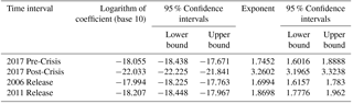
In Fig. 6a, the hourly mean power of the dominant eigenvector is shown for the entire 2017 interval of record as a function of discharge. There is significant variability in hourly mean power for intervals with low discharge, possibly related to other sources of noise including anthropogenic noise created during spillway repair efforts, wind noise, or distant fluvial or marine sources. Below a discharge of approximately 200 m³ s⁻¹, there does not appear to be a relationship between dominant eigenvector power and discharge. We therefore interpret 200 m³ s⁻¹ as the threshold discharge above which signals emanating from the Oroville spillway become the dominant source of seismic. Figure S2 in the Supplement shows the dominant eigenvector power for all discharges. We limit our analysis of scaling between discharge and mean hourly eigenvector power to hours when discharge exceeded 200 m³ s⁻¹, and to hours with spillway use as reported by the California Department of Water Resources. In Fig. 6a, the scaling relationship between discharge (Q) and power before the crisis is P_W∝Q^1.75. After the spillway defect occurs, the scaling exponent is greater, with P_W∝Q^3.26. Figure 6b and c display the power-discharge relationships for the 2006 and 2011 release periods. The scaling exponent for these release events is similar (P_W∝Q^1.70–1.87) to the pre-crisis scaling, although there is more scatter in the 2011 seismic record. The coefficients, exponents, and estimates of uncertainty are provided in Table 1. The change in the scaling relationship between discharge and seismic power is consistent with the inferred increase in turbulent energy dissipation following the damage to the flood control spillway (see discussion).

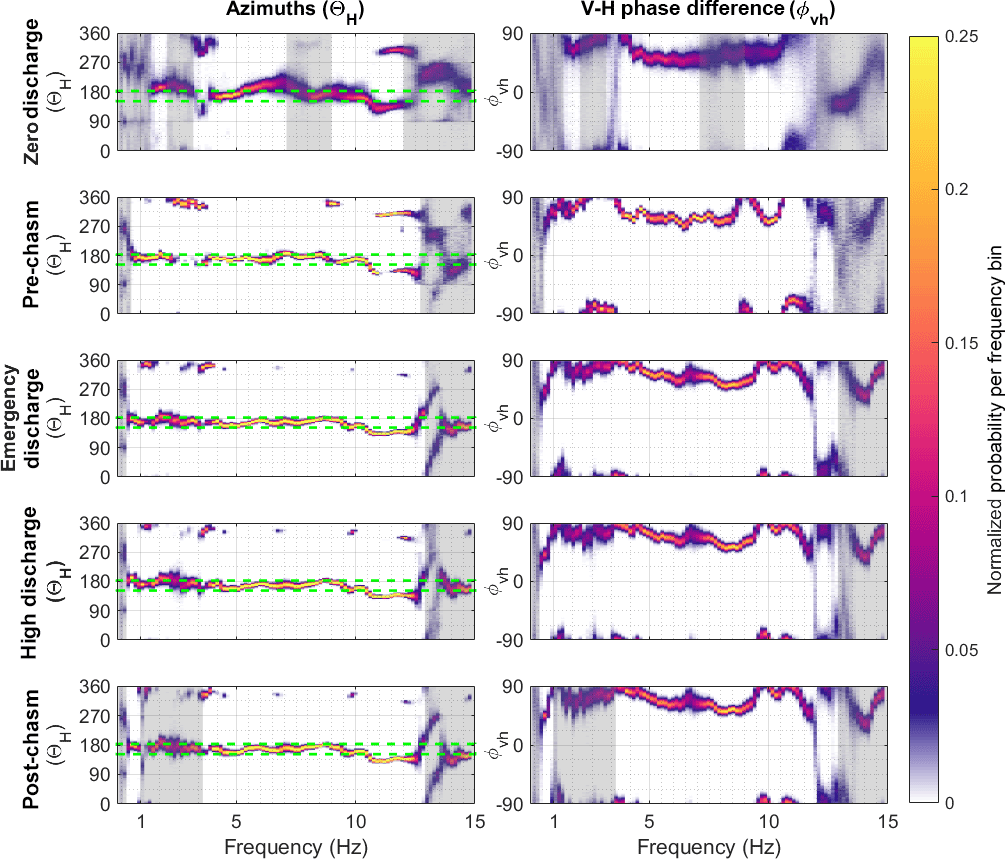
Figure 7 Two polarization attributes for the five time intervals of interest are presented in two-dimensional histograms. Dashed green lines in the left column indicates the azimuth range of the spillway relative to the seismometer (See Fig. 1). Each hour within the time interval of interest has a polarization value at 7201 frequencies. These are distributed among 100 bins evenly spaced in frequency, and are colored by normalized probability. The polarization attributes for the three intervals of interest after the spillway damage are similar, and differ dramatically from the attributes in the pre-crisis interval. Polarization attributes are interpretable only when the degree of polarization is sufficiently great (β² > 0.5). Regions shaded grey indicate frequencies at which β² < 0.5 and the values are not interpretable.

4.2 Polarization attributes

To examine the potential source of seismic waves across a range of frequencies, we display the azimuth and vertical–horizontal phase difference in Fig. 7 for the five time intervals of interest. All five polarization attributes are provided in the Supplement. To evaluate the variability of polarization within each constant discharge interval, the probability density functions (PDFs) of all the hourly polarization results are plotted together in Fig. 7. In the figure, the polarization attributes are binned into 100 evenly spaced frequency bins from 0.1 to 15 Hz and the PDFs are normalized so that within each frequency bin, the probability sums to one. The brighter colors indicate highly focused attributes and the darker colors indicate broadly distributed attributes. When ground motion is insufficiently polarized, polarization attributes are not interpretable (Samson, 1983). We select a cutoff β² at 0.5 as our threshold criterion for interpreting polarization attributes; Koper and Hawley (2010) selected a β² cutoff value of 0.6. Frequency ranges that are not interpretable by this criterion are shaded grey in Fig. 7.

The three time intervals after the spillway damage occurred (“Emergency discharge”, “High discharge”, and “Post-chasm discharge”) display similar polarization attributes. The discharge through the emergency spillway weir, which reached a maximum of 360 m³ s⁻¹, is masked by the ∼ 1500 m³ s⁻¹ discharge in the primary spillway during this time (California Department of Water Resources, 2017c). When compared to the time intervals with discharge, the “Zero discharge” time interval contains less polarized three-component motion. Based on our threshold criterion, polarization attributes are not interpretable for a broad range of frequencies. At zero discharge, only polarization attributes at frequencies near 1, 4, and 10 Hz are interpretable, representing the ambient noise environment of the station. During the four intervals with non-zero discharge, a broad range of frequencies below 12 Hz are interpretable. There is a significant increase in polarization after the flood control spillway damage in a narrow frequency band around 0.7 Hz. From 1 to 5 Hz, the β² decreases from the “Pre-chasm” discharge to the three “Post-chasm” discharge intervals. The decrease in β² may be attributable to a mixing of seismic sources contributing to the ground motion (see discussion).

4.3 Horizontal azimuth

To resolve the potential changes in seismic source location resulting from the flood control spillway damage, we evaluate the horizontal azimuth, which is computed for each frequency bin in Fig. 7. The horizontal azimuth (Θ_H) of the dominant particle motion ellipsoid represents the azimuth of the incoming wave if the motion is Rayleigh-like or a P-wave. Park et al. (1987) and Koper and Hawley (2010) caution interpreting Θ_H as the azimuth if the horizontal–horizontal (ϕ_hh) phase difference is within 20^∘ of ±90^∘, because the azimuth is not defined for a horizontal circular motion. At zero discharge, the horizontal azimuth is somewhat variable; multiple sources of seismic energy with equal amplitudes may be present in the absence of spillway discharge (Fig. 7). During the time intervals with spillway discharge, horizontal azimuth is generally consistent from 5–8 Hz, then it stair steps to lower azimuths at frequencies near 10 Hz.

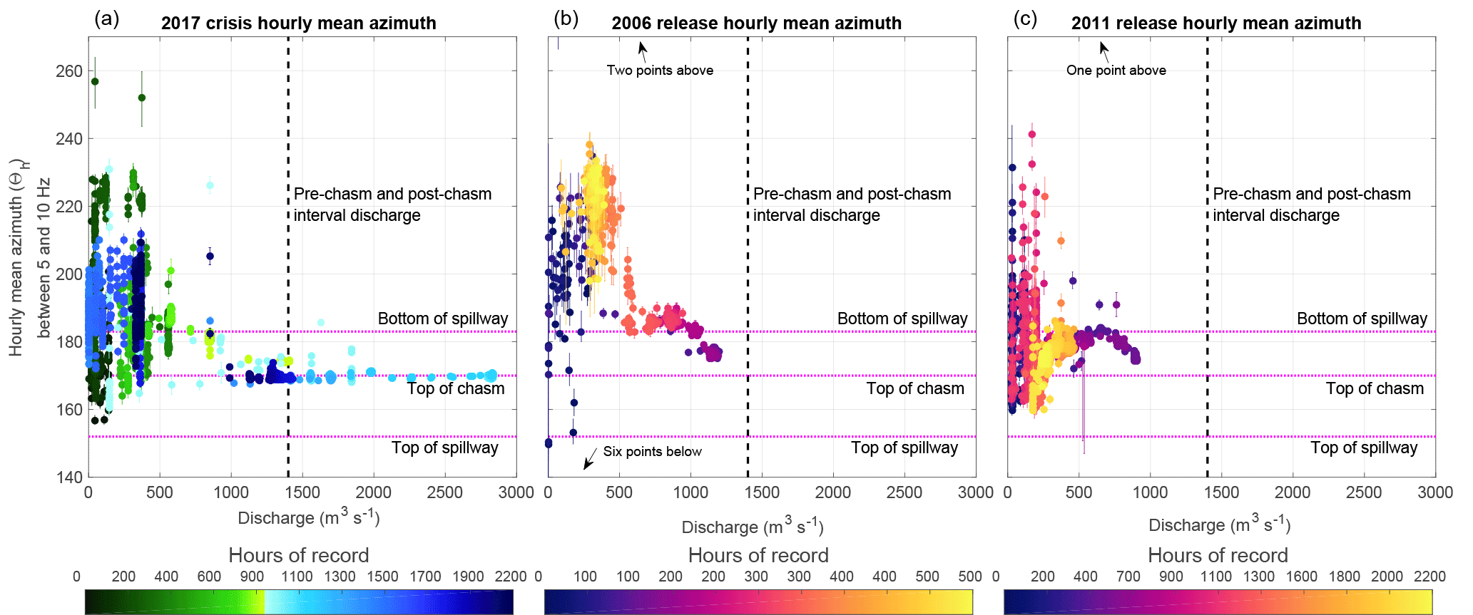
Figure 8 In the 5–10 Hz band, hourly mean azimuth (Θ_H) is displayed in panels (a–c), with 95 % error bars. The mean azimuth is highly variable for discharge less than 500 m³ s⁻¹ for the flood control releases in 2017 (a), 2006 (b), and 2011 (c). In panel (a), during the “Pre-chasm” time interval shaded green, the mean horizontal azimuth values point to the bottom of the flood control spillway (183^∘, Fig. 1c). After the high releases have formed a chasm that starts in the middle of the flood control spillway, the azimuths consistently point to the channel midpoint. The “Post-chasm” azimuth when discharge is approximately 1400 m³ s⁻¹ is noticeably distinct from the “Pre-chasm” flows around 1400 m³ s⁻¹. During times when the channel is undamaged (b, c), the mean azimuth is sensitive to changes in discharge as turbulence develops in the middle of the flood control spillway. Due to the 180^∘ indeterminacy, Θ_H shown in this figure is constrained between 90 and 270^∘, the direction of the outflow channel.

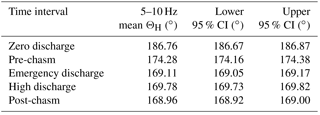
In order to compute summary statistics of the horizontal azimuth, we select a frequency band of 5–10 Hz. This band has a degree of polarization above 0.5 for all time intervals with discharge and has a horizontal phase angle difference (ϕ_hh) outside of 20^∘ from 90/−90^∘ (for which the azimuth is not defined). As directional data such as azimuth require special statistical treatment, we employ the CircStat Matlab toolbox for circular statistics to compute an hourly mean azimuth with 95 % confidence intervals (Berens, 2009). Due to the 180^∘ ambiguity in azimuth estimates, we add or subtract 180^∘ from the mean azimuths that are < 90 or > 270^∘. This choice is supported by the strong relationship observed between power and changes in discharge which indicate that the flood control spillway channel (between 152 and 183^∘) is the primary seismic source across a broad range of frequencies (See Fig. 1c). We compute the uncertainty on the mean using 2000 random bootstrap samples with replacement. Table 2 displays the mean 5–10 Hz azimuth within each time interval, with 95 % confidence interval error bars. Figure 8a displays the average hourly 5–10 Hz Θ_H as a function of flood control spillway discharge, with hourly 95 % confidence intervals for the 2017 period. For comparison, Fig. 8b and c display the same data for the 2006 and 2011 release periods.

At low spillway discharges, the horizontal azimuth values are variable but generally point southward towards the Feather River and town of Oroville (183 to 250^∘), whereas during time intervals with elevated discharge the azimuth values point more consistently toward the flood control spillway channel, centered at 171^∘. During times when the spillway is undamaged, the hourly mean azimuth changes systematically with spillway discharge above about 500 m³ s⁻¹. The hourly mean azimuth moves from the base of the flood control spillway towards the middle of the spillway with increasing discharge. After the erosion damage begins (Fig. 8a), the azimuths point more towards the top of the chasm, where a large waterfall develops as a result of the erosion damage. Above 1000 m³ s⁻¹, the azimuths point consistently to the middle of the outflow channel. The azimuths around a discharge of 1400 m³ s⁻¹ are different before the erosion crisis occurred (bright green shading) and after a chasm is present (dark blue shading). This distinction indicates that the FDPA-derived azimuths are sensitive to changes in the turbulence regime under normal spillway operation and when erosion damage is present (see discussion in Sect. 5).

Table 2 Distribution statistics for the mean azimuth within the five time intervals of interest. The 95 % confidence intervals (CI) on the mean are determined by collecting 2000 random bootstrap samples with replacement.

4.4 Incident angle

The vertical angle of the dominant eigenvector represents the incidence angle of the incoming wave for body waves or tilt of elliptical motion for Rayleigh waves. Park et al. (1987) and Koper and Hawley (2010) caution interpreting this metric if ϕ_vh is within 20^∘ of ±90^∘, because the vertical incidence angle of vertical circular motion is not defined. At a broad range of frequencies this criterion is not met during time intervals with discharge (see Sect. 4.5). In all five time intervals of interest, the Θ_V values are highly variable (see Supplement).

4.5 Vertical–horizontal phase difference

To evaluate the possible surface wave type (i.e., Rayleigh or Love), we assess the vertical–horizontal phase difference. For a Rayleigh wave in an isotropic medium, the vertical–horizontal phase difference will be ±90^∘. In certain anisotropic structures, the vertical–horizontal phase difference for a Rayleigh wave will deviate from ±90^∘ (Crampin, 1975). In Fig. 7, the vertical–horizontal phase angle (ϕ_vh) is consistently near ±90^∘ for frequencies below 5 Hz when discharge is occurring, which is consistent with a Rayleigh-like wave. At frequencies of up to 8 Hz, which account for most of the power, there is a decreasing vertical–horizontal phase angle to approximately 50^∘. At 8 Hz, the vertical–horizontal phase angle is 50^∘ in the “Pre-chasm” time interval and near 90^∘ in the “Post-chasm” time interval. These deviations from ±90^∘ are unexpected and explored in Sect. 4.7.

4.6 Horizontal phase difference

For all of the time intervals of interest, the ϕ_hh is between ±180 and ±90^∘ for most frequencies, suggesting horizontal elliptical particle motion. At 8 Hz, the “Pre-chasm” and “Post-chasm” time intervals seem to change from near −180 to near −115^∘ phase difference, suggesting a change from linear horizontal motion to more elliptical horizontal motion at frequencies near 8 Hz.

4.7 Topographic effects on vertical–horizontal phase angle

We observe consistent deviations from the expected vertical–horizontal phase difference of ±90^∘ between 5 and 10 Hz, even during the “Pre-chasm” interval (Fig. 7). To investigate the possible reasons behind these deviations, we consider the effect of the irregular hillside topography on the polarization results by computing synthetic seismograms using the 2-D spectral-element solver package SPECFEM2D 7.0.0 (Tromp et al., 2008; Komatitsch et al., 2012). All geospatial data were processed in ESRI ArcMap 10.4. First, a 2013 1∕3 arcsec resolution digital elevation model was acquired from the USGS National Elevation Dataset at http://www.nationalmap.gov (last access: 22 August 2017). The raster was reprojected to Universal Transverse Mercator Zone 10N to acquire northing and easting coordinates in a conformal (angle-preserving) coordinate system. Elevation data (in meters, NAVD 88) were extracted from each grid cell along a profile line between the top of the spillway erosion damage and the seismometer in this study. The topographic profile was meshed into the model domain using the built-in xmeshfem2d program. To minimize model boundary effects, the lower model boundary extends over 4 km below the surface. We also generated a rectangular model grid with a flat surface in SPECFEM2D for comparison. We select a density of 2700 kg m⁻³, increase P wave velocity linearly with depth from 4 km s⁻¹ at the surface to 6 km s⁻¹ at 4 km depth, and assume a Poisson solid.

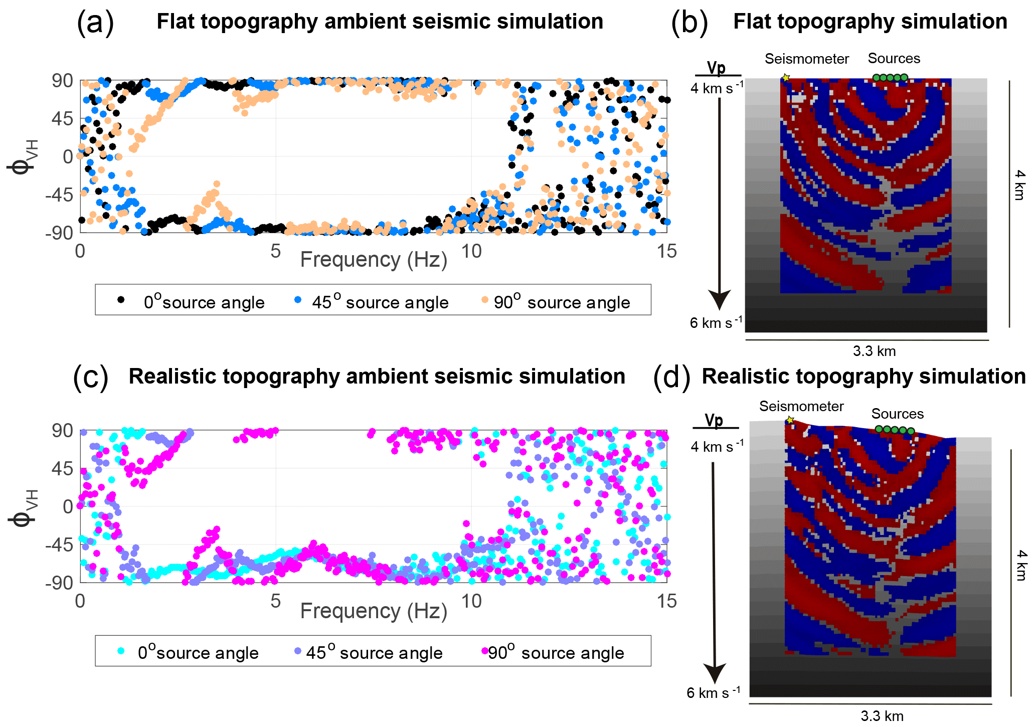
Figure 9 Polarization attributes computed using FDPA of synthetic seismograms computed using SPECFEM2D are shown in panels (a) and (c); with corresponding simulated topographies. The distributed source of the spillway is approximated by five sources spaced 100 m apart with a source frequency of 5–10 Hz. Random noise was added to the results of the simulation to approximate background seismic noise. Panels (a) and (b) display the horizontal component seismic wave field during a single time step in each simulation. In the flat topography simulation (a), the vertical–horizontal phase difference is closer to ±90^∘ than in the simulation that includes the realistic hillslope topography (c). With a vertically incident force (0^∘ source angle), the phase difference is lowest, while with increasing source angle, the vertical motion becomes less like a classical Rayleigh wave below 5 Hz.

In both the topographic and flat surface simulations, continuous signals were used as the seismic source, and were applied independently at five locations spaced 100 meters apart and representing a spatially distributed source along the Oroville flood control spillway channel projected onto a 2-D profile line (See Supplement Fig. S3). Each independent source consists of a four-minute random signal varying between zero and one filtered using a second-order Butterworth filter between 5 and 10 Hz. Deviations from Rayleigh-like wave polarizations are observed at these frequencies (Fig. 7). The angle of incidence of the continuous seismic source was varied between 0, 45, and 90^∘ with respect to the vertical. Synthetic seismograms were simulated at the location of the BK ORV seismometer, with random noise added to the resulting synthetic seismograms to approximate background seismic sources. As the simulations are carried out in a 2-D geometry, the results may only be used to evaluate the effect of topography on vertical–horizontal phase differences. The results of the simulations show that for vertically incident fluctuating forces applied along the Oroville flood control spillway , the particle motion is Rayleigh-like (vertical–horizontal phase difference is near ±90^∘) for a flat topography (Fig. 9a). As the fluctuating force is applied at angles of 45 and 90^∘ to the surface, the vertical–horizontal phase becomes less Rayleigh-like below 5 Hz. Realistic topography also appears to significantly affect the particle motion, which becomes less Rayleigh-like, as vertical–horizontal phase differences decrease from ±90 to ±45^∘ between 5 and 10 Hz (Fig. 9c). This is consistent with the conversion of Rayleigh energy to body-waves as the seismic waves propagate up a non-uniform slope (e.g., McLaughlin and Jih, 1986).

5 Discussion

The changing geometry of the flood control spillway and the increase in flow turbulence during the Oroville Dam erosion crisis are reflected in the FDPA results, most notably in dominant eigenvector power and horizontal azimuth. During the crisis, large volumes of material (1.3 × 10⁶ m³ according to our analysis of lidar data) were transported, which previous work has shown can contribute to the overall seismic signal (Tsai et al., 2012). Therefore, one might expect bedload transport to be the dominant source of seismic energy. Yet, there are compelling lines of evidence that suggest that the majority of the signal is flow-generated. First, the fastest rate of material transport on the Oroville flood control spillway was likely during the early part of the crisis timeline. Water entering the flood control spillway is from the surface of the reservoir. Unlike a natural river, it does not carry bedload or coarse suspended sediment, so any transported material must be entrained from the spillway itself or the adjacent hillside. Early in the Oroville Dam crisis, weathered saprolite and concrete blocks were undercut and eroded, while later in the crisis, the water from the spillway flowed over harder volcanic rocks. If the seismic signal was generated by a transient transport pulse, we would expect a rapid jump and decay in the amplitude of the seismic waves coming from the spillway. If greater erosion occurred at the beginning of the crisis and if transported material were the primary source of the seismic energy, we would expect clockwise power-discharge hysteresis in this system. Instead, we observe counterclockwise hysteresis in this relationship. Although our analysis does not enable us rule out all other seismic sources such as material transport, we think that the changes in FDPA results are consistent with changes in the turbulent flow regime caused by erosional changes in channel geometry.

Counterclockwise hysteresis in the discharge–power relationship is consistent with the increased channel roughness and larger scaling of macroturbulent eddies resulting from the Oroville Dam erosion crisis. Because of the dissimilarity of the system to a natural channel, we are unable to fully implement theoretical models of fluvial seismic energy generation, but we are able to examine whether the scaling relationships within these models are consistent with our data. The theoretical scaling relationship between water-generated vertical component power (P_W) and discharge (Q) for water turbulence alone with a simple channel geometry is P_W∝Q^1.25 (Gimbert et al., 2014, 2016). Roth et al. (2017) found a P_W∝Q^1.49–1.93 in the 35–55 Hz band. In the 0.5 to 1 Hz band for the smooth channel (2006, 2011, and pre-crisis 2017) the observed scaling of dominant eigenvector power and turbulence is P_W∝Q^1.69–1.88, similar to the scaling observed by Roth et al. (2017). After the spillway erosion crisis, the scaling exponent is much higher (P_W∝Q^3.28). We observe similar scaling relationships for the vertical component power (without polarization analysis), with 2006, 2011, and pre-crisis 2017 scaling as P_W∝Q^1.74–1.98 and post-crisis 2017 scaling as P_W∝Q^3.26.

The increased scaling exponent following the crisis likely corresponds to the addition of new sources of turbulent energy dissipation generated from the rougher channel morphology associated with exposed bedrock and waterfall. For a uniform turbulent flow, as expected in the hydraulically smooth, constant-width channel geometry present during the 2005–2006 flood, discharge is log-linearly related to flow depth according to the “law of the wall”, and ground motion is generated by fluctuating forces applied by scaled eddies within the flow, analogous to the processes described by Gimbert et al. (2014). After damage is created in the channel, several mechanisms likely increase the energy dissipated by the flow at a given discharge. The first is that the erosion damage introduced a steep vertical drop in the base of the channel, developing a waterfall. A waterfall will violate assumptions in the Gimbert et al. (2014) model formulation and lead to greater water velocities (from free fall) impacting the bed than would be found in a continuous turbulent channel flow. Second, the irregular channel shape resulting from erosion provides obstructions to the flowing water that create local pressure gradients around the obstacles. These pressure gradients cause a deflection in the flow and an increase in the shearing between flows of different velocities, increasing the energy dissipated by the turbulence in the flow. Third, erosion during the 2017 event incised a 47 m-deep, V-shaped channel, which increased flow depths for the same discharge and changed the distribution of shear stresses applied to the bed. Greater flow depths would also allow for larger eddies to form. Our results suggest that the additional energy dissipated by these forms of turbulence is observed as an increase in the scaling relationship between discharge and seismic power. Our observations support the use of the exponent in the P_W∝Q power function to observe changing channel geometries in supply-limited fluvial systems (as in Gimbert et al., 2016), but are unable to identify a particular source mechanism.

The FDPA polarization attributes reveal the seismic character of open channel turbulent flow, which is distinct from the background seismic character (“Zero discharge” interval) across a broad range of frequencies (Fig. 7; Supplement). The three time intervals with discharge following the flood control spillway damage have similar polarization attributes, while the “Pre-chasm” time interval is identifiable by a higher degree of polarization at frequencies below 3 Hz, and the absence of a 0.7 Hz sharp peak in dominant eigenvector power (Fig. 4) and degree of polarization. The decrease in degree of polarization is consistent with mixed seismic waveforms from multiple sources (Rayleigh, Love, P, and S) being introduced by the chasm channel complexity and increased turbulent energy dissipation. We are unable to attribute a source to the 0.7 Hz anomaly, but we note that at around 0.7 Hz we observe azimuths of about 180^∘, an incidence angle of about 25^∘ from vertical, a vertical–horizontal phase difference about 45^∘, and broadly distributed horizontal–horizontal phase difference. The azimuth is consistent with the base of the flood control spillway, though the vertical incidence is steeper than the 13^∘ slope of the hillside.

The greatest hysteresis in the power and discharge relationship is observed at low frequencies (0.5 to 1 Hz), however, the greatest hysteresis in azimuth is observed at higher frequencies (5–10 Hz). This difference may be due to the greater sensitivity to source location that is provided by the higher frequencies, which have shorter wavelengths. For a Rayleigh wave traveling through rock at approximately 3 km s⁻¹, the wavelength of a 0.5–1 Hz wave is 6 to 3 km, significantly longer than the 1 km long flood control spillway, meaning that changes in source location along the spillway may not be observable in azimuths computed at low frequencies. However, at 5 to 10 Hz, the wavelength is 0.6 to 0.3 km, which is sufficient to identify distinct segments of the flood control spillway.

The hourly 5–10 Hz mean azimuths (Fig. 8) are sensitive to changes in discharge even when no damage is present (Fig. 8b and c). Aerial photographs of the spillway at a range of discharges reveal that the location of the transition from smooth to visibly white and aerated turbulent flow in the bottom half the spillway is sensitive to changes in discharge (See Fig. S5 in the Supplement). In the dam engineering literature, the onset of surface turbulence is referred to as the inception point and represents where the turbulent boundary layer reaches the free surface (Hunt and Kadavy, 2010a, b). The aerated flow region downstream of the inception point indicates increased energy dissipation. Due to the geometry of the spillway channel with respect to the seismometer, as the inception point moves up the spillway channel it approaches the seismometer. We expect the closest portion of the aerated flow region to be the largest source of seismic energy under undamaged conditions; seismic energy excited further from the seismometer will be subject to more geometrical spreading and attenuation.

Figure 10 Mean azimuths for the five time intervals of interest mapped onto aerial imagery reveal the “Emergency discharge”, “High discharge”, and “Post-chasm” mean azimuths point to the top of the spillway damage, where a steep drop creates a waterfall. The location of the initial damage, shown as a triangle, is estimated from photographs of the damage (see Supplement). The location of the damage top, shown as a circle, is estimated from aerial photography and high-resolution lidar points collected after most of the damage occurred.

The hourly 5–10 Hz mean azimuths are also sensitive to changes throughout the dam erosion crisis. During the 2017 period, the “Pre-chasm” and “Post-chasm” time intervals have a statistically significant difference in mean azimuth of 5.32^∘. The “Emergency discharge”, “High discharge”, and “Post-chasm” time intervals have mean azimuths within a 1^∘ range. To interpret these results, we reviewed available aerial photography throughout the Oroville crisis and extracted an elevation profile along the length of the flood control spillway using the lidar measurements provided by the California Department of Water Resources (CADWR). The imagery review reveals that the top of the erosion damage propagated upstream a distance of approximately 120 m (approx. 2.8^∘ azimuth) between 7 and 27–28 February (Fig. 10). The upstream end of the erosion damage forms a waterfall. FDPA results from the “Emergency discharge”, “High discharge”, and “Post-chasm” time intervals are able to identify the waterfall at the top of the erosion damage. The “Emergency discharge” time interval has an azimuth within 1^∘ of the immediately following “High discharge” interval, indicating that 360 m³ s⁻¹ released through the emergency spillway did not generate sufficient energy to mask the concurrent flood control spillway releases at that time.

The particle motion of seismic waves produced by the Oroville Dam spillway is mostly Rayleigh-like, particularly at frequencies below 3 Hz, though we also observe consistent deviation from the expected Rayleigh ϕ_vh values (−90 and 90^∘) at frequencies from 5–10 Hz. This could be explained by the presence of anisotropy (Crampin, 1975) or Love and/or body waves, which induce shifts in ϕ_vh but our SPECFEM2D modeling indicates that realistic topography is also a viable explanation for the polarization attributes we observe, specifically ϕ_vh. Therefore, our analysis is limited to time varying changes in polarization attributes rather than interpreting the surface and/or body waveforms created by the flood control spillway. We see the greatest difference in ϕ_vh and ϕ_hh between the “Pre-chasm” and “Post-chasm” time intervals below 3 Hz and in the 9–11 Hz band, potentially indicating that more Rayleigh energy is produced at these frequencies after the channel geometry becomes more eroded and incised.

6 Conclusion

Our analysis of the seismic data collected during the Oroville Dam erosion crisis identified several techniques that are potentially useful for dam spillway monitoring and can be applied to fluvial studies. We evaluated the single-station FDPA method to locate the region of greatest flow turbulence. To our knowledge, this is the first application of FDPA methods to analysis of a hydrodynamic signal. We were able to resolve changes in the mean azimuth of the turbulence-generated 5–10 Hz seismic waves under normal spillway conditions (2006 and 2011 release periods) when varying discharge and velocity generate changes in the location of the aeration zone inception point. During high spillway discharges and the onset of spillway damage (2017 crisis), the data analysis techniques were used to pinpoint the upstream location of spillway erosion as identified by the increased turbulence. This technique is promising for fluvial studies to identify potential seismic energy interference from nearby waterfalls (i.e., Roth et al., 2016) or in otherwise noisy study environments. The vertical–horizontal phase difference of the spillway-generated energy is consistent with a Rayleigh wave propagating up the dam non-uniform hill slope.

We find that for constant discharge conditions and varying amounts of spillway damage and associated macroturbulence, counterclockwise hysteresis in the discharge–seismic power relationship indicates that the turbulent structures created by the spillway damage excite seismic energy more effectively. This observation is consistent with the increased energy dissipation by macroturbulent eddies and stepped flows considered in spillway design (Hunt and Kadavy, 2010a). This observation is also consistent with the fluvial geomorphology literature that argues a significant proportion of total energy dissipation is caused by macroturbulent eddies in natural rivers (Leopold et al., 1960; Prestegaard, 1983; Powell, 2014). Therefore, seismic monitoring may be a tool to quantify macroturbulent eddies and associated flow resistance in complex natural channels. The results of this study are consistent with those of Roth et al. (2017), who suggested changes in channel morphology as a cause of water turbulence-associated hysteresis in natural channels. This study also implies that the Gimbert et al. (2014) model will underpredict seismic energy released in rivers with irregularly shaped channels, waterfalls, and macroturbulent eddies. In this study, we observed that the generation of irregular channel morphology by damage to the spillway produced greater scaling exponents in the seismic power discharge relationship than the pre-damaged spillway, which produced scaling exponents similar to those predicted by the Gimbert et al. (2014) model.

Although results of this work can be applied to spillway monitoring and natural channel observations, we highlight several limitations of the methods used in this study. The long intervals of constant or known discharge in spillway operations are dissimilar from the sharp increases and decreases in discharge observed in most rivers hydrographs. In this study, we assumed that during intervals of constant discharge flow turbulence generated seismic motions with the same polarization attributes. Therefore, uncertainty was estimated by documenting the variability of polarization attributes during these time intervals of constant discharge. Due to the hazardous conditions surrounding the spillway channel, inferences on the mechanisms and degree of turbulence are limited to interpretations of aerial photography. This study was limited to the hourly resolution of reported discharge and the sampling frequency and sensitivity of the broadband seismometer in the study. For natural rivers, further research is needed to understand the appropriate time window length and sampling frequency to characterize turbulence at various scales.