the Creative Commons Attribution 4.0 License.
the Creative Commons Attribution 4.0 License.
 | 17 Sep 2019
Introducing PebbleCounts: a grain-sizing tool for photo surveys of dynamic gravel-bed rivers
Benjamin Purinton
Bodo Bookhagen
Grain-size distributions are a key geomorphic metric of gravel-bed rivers. Traditional measurement methods include manual counting or photo sieving, but these are achievable only at the 1–10 m2 scale. With the advent of drones and increasingly high-resolution cameras, we can now generate orthoimagery over hectares at millimeter to centimeter resolution. These scales, along with the complexity of high-mountain rivers, necessitate different approaches for photo sieving. As opposed to other image segmentation methods that use a watershed approach, our open-source algorithm, PebbleCounts, relies on k-means clustering in the spatial and spectral domain and rapid manual selection of well-delineated grains. This improves grain-size estimates for complex riverbed imagery, without post-processing. We also develop a fully automated method, PebbleCountsAuto, that relies on edge detection and filtering suspect grains, without the k-means clustering or manual selection steps. The algorithms are tested in controlled indoor conditions on three arrays of pebbles and then applied to 12 × 1 m2 orthomosaic clips of high-energy mountain rivers collected with a camera-on-mast setup (akin to a low-flying drone). A 20-pixel b-axis length lower truncation is necessary for attaining accurate grain-size distributions. For the k-means PebbleCounts approach, average percentile bias and precision are 0.03 and 0.09 ψ, respectively, for ∼1.16 mm pixel−1 images, and 0.07 and 0.05 ψ for one 0.32 mm pixel−1 image. The automatic approach has higher bias and precision of 0.13 and 0.15 ψ, respectively, for ∼1.16 mm pixel−1 images, but similar values of −0.06 and 0.05 ψ for one 0.32 mm pixel−1 image. For the automatic approach, only at best 70 % of the grains are correct identifications, and typically around 50 %. PebbleCounts operates most effectively at the 1 m2 patch scale, where it can be applied in ∼5–10 min on many patches to acquire accurate grain-size data over 10–100 m2 areas. These data can be used to validate PebbleCountsAuto, which may be applied at the scale of entire survey sites (102–104 m2). We synthesize results and recommend best practices for image collection, orthomosaic generation, and grain-size measurement using both algorithms.
- Article
(13146 KB) - Full-text XML
-
Supplement
(20611 KB) - BibTeX
- EndNote


Gravel-bed rivers transport water, nutrients, and sediment downstream, linking high mountains with populated forelands. The grain-size distributions – and associated percentile diameters, such as the D50 and D84 – in a river reach are fundamental geomorphic metrics of these systems (e.g., Shields, 1936; Parker et al., 1982; Church et al., 1998). They are used to characterize aquatic habitats (e.g., Kondolf and Wolman, 1993), assess the impacts of human infrastructure like dams (e.g., Kondolf, 1997; Grant, 2012), calibrate theoretical models of river transport and erosion (e.g., Sklar et al., 2006; Attal and Lavé, 2006; Attal et al., 2015; Dunne and Jerolmack, 2018), and explore natural phenomena such as downstream fining (e.g., Paola et al., 1992; Ferguson et al., 1996; Rice and Church, 1998; Gomez et al., 2001; Chatanantavet et al., 2010; Lamb and Venditti, 2016), which is essential for nutrient transport and ecological diversity.
Accurate grain-size measurement is elusive in nature given the heterogeneity of gravel-bed rivers, particularly in steep mountain catchments where the range of grain sizes is large. Traditionally, grain-size distributions have been gathered via physical clast measurement and counting along grids (Wolman, 1954), lines (Wohl et al., 1996), or in ∼1 m2 patches (Bunte and Abt, 2001), all truncated at some lower observable limit (e.g., Rice and Church, 1998). Not only are these techniques time-consuming, prone to operator bias, and disruptive to the environment, but they also require large (hundreds of pebbles) sample sizes to accurately estimate the characteristic nature of the grains in each location (Wolcott and Church, 1991).
In light of this, measurement from photographs is an attractive option for increasing sample size and decreasing fieldwork, while covering larger areas. Increasingly affordable high-resolution – 12- to 24-megapixel – cameras allow the collection of high-quality photo surveys via structure from motion with multi-view stereo (SfM-MVS) (Smith et al., 2015; Eltner et al., 2016) at scales of entire river cross sections or reaches with resolutions at, or exceeding, 1 cm pixel−1 (e.g., Woodget and Austrums, 2017). Even higher-resolution (1 mm pixel−1) river surveys can be accomplished with low-flying unmanned aerial vehicles (UAVs) (e.g., Carbonneau et al., 2018), pole-mounted cameras, or using handheld imagery.
We build on previous work and introduce the addition of color-space clustering techniques to present efficient new semi-automated (PebbleCounts) and fully automated (PebbleCountsAuto) algorithms for grain sizing from imagery in high-energy mountain rivers. Our algorithms are built on Python with a few popular libraries and are open source. The instructions and code can be accessed at https://github.com/UP-RS-ESP/PebbleCounts (last access: 12 September 2019) (Purinton and Bookhagen, 2019). In this study, we present previous work on grain-size measurement from rivers and our motivation for new developments. The processing chains of PebbleCounts and PebbleCountsAuto are then discussed. We test the algorithms in controlled conditions and then in a more challenging field setting in the northwestern Argentine Andes. The limits and caveats of the method are discussed using imagery of varying resolution, and suggestions for photo collection and processing are provided.
1.1 Prior studies
Modern digital grain sizing is divided into texture- and segmentation-based image-processing methods, as opposed to previous manual digitization (e.g., Kellerhals and Bray, 1971; Ibbeken and Schleyer, 1986). Many texture methods rely on the relationship between grains and their shadowed interstices to derive size estimates over image windows. Examples include semivariance (Verdú et al., 2005; Carbonneau et al., 2003, 2004; Carbonneau, 2005), entropy or inertia calculated from gray-level co-occurrence matrices (Haralick et al., 1973; Carbonneau et al., 2004; Carbonneau, 2005; Dugdale et al., 2010; de Haas et al., 2014; Woodget and Austrums, 2017; Woodget et al., 2018), and autocorrelation (Rubin, 2004; Warrick et al., 2009; Buscombe et al., 2010). These methods only provide one estimate of grain size (e.g., D50), which often requires site-specific calibration.
Buscombe (2013) achieved full grain-size distribution measurements using wavelet decomposition and published an open-source Python tool, pyDGS. This is a texture method that has been designed for the analysis of thin sections or beach sands and requires each grain to be fully resolvable and the distributions to be fairly homogeneous in size and shape. Additional texture methods rely on the 3-D texture (or roughness) of point clouds to relate the variance of bed-scale topography to average grain size (Brasington et al., 2012; Rychkov et al., 2012; Westoby et al., 2015; Woodget and Austrums, 2017; Bertin and Friedrich, 2016); however, these techniques also require site calibration, and the relationships have been found to vary widely (Pearson et al., 2017).
In contrast to texture methods, the focus of segmentation is the full delineation and measurement of every visible grain. Segmentation is error prone in images that contain overlapping grains, a large range of grain sizes including sand patches, changes in land cover (e.g., vegetation), pebbles that are highly irregular in shape (non-ellipsoid), pebbles with intragranular color variations or texture such as veins or fractures, and in which shadowing is irregular. Herein, we refer to these factors collectively as image complexity. Furthermore, segmentation-based methods also require high-spatial-resolution point clouds or images that resolve the specific grain geometries. The benefits are that segmentation does not require any site calibration besides knowledge of the image scale and it provides a full grain-size distribution and all the commonly used percentiles (). Published methods by Butler et al. (2001), Sime and Ferguson (2003), and Graham et al. (2005a, b) all rely on edge detection followed by watershed segmentation and ellipse fitting to each separate grain to get the long (a) and intermediate (b) axes. Detert and Weitbrecht (2012) added some sophistication to the algorithm of Graham et al. (2005a, b) and provide a free – though closed-source – application called Basegrain for Matlab™, which has become a standard tool (e.g., Bertin and Friedrich, 2016; Bertin et al., 2017; Langhammer et al., 2017; Carbonneau et al., 2018).
1.2 Motivation
Watershed segmentation is effective for interlocking, uniformly colored, oblate grains; however, energetic gravel-bed rivers in mountains often have more complex grain compositions with intragranular variation, irregular shadowing, and a large range of sizes. The automated watershed methods proposed suffer from oversegmentation, grain misidentification, and the need for significant, time-consuming post-processing (e.g., in Basegrain with the split, merge, and delete tools) when applied to complex images. These issues limit their application to areas <10 m2.
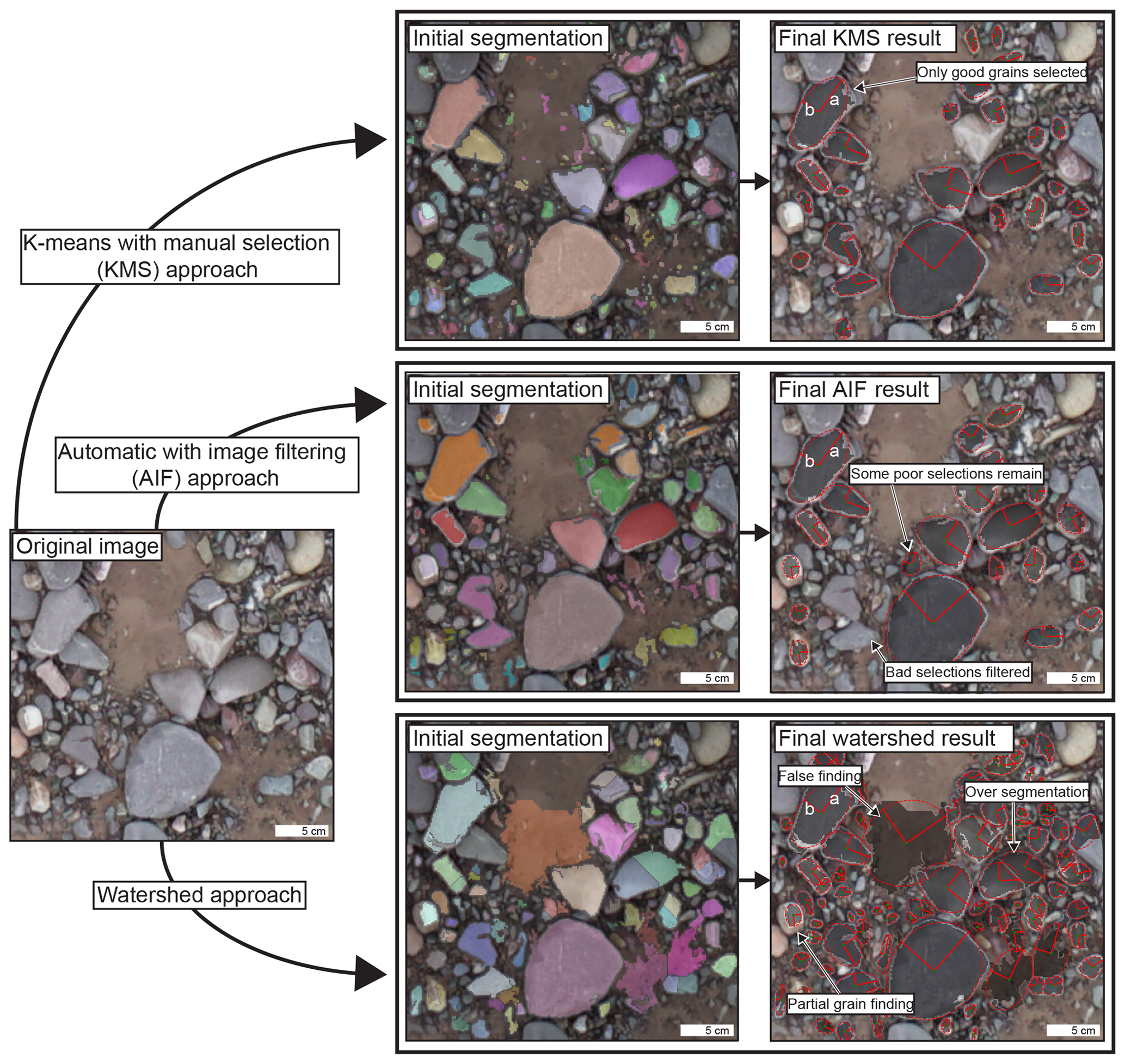
Figure 1Difference between our k means with manual selection (KMS) and automatic with image filtering (AIF) approaches versus a fully automated watershed segmentation approach on a gravel image from a high-mountain river. The a and b axes of each grain mask are found via an ellipse fit to the same area. Fewer grains are found in the KMS and AIF results, and there is still some misidentification in the case of AIF but less than in the watershed result.
Thus, we are motivated to develop a new semi-automated technique that uses k-means clustering of pixels and rapid manual selection of well-defined grains, herein referred to as the k means with manual selection (KMS) or PebbleCounts approach, and a fully automated version that uses filtering of suspect grains, herein referred to as the automatic with image filtering (AIF) or the PebbleCountsAuto approach (Fig. 1). By avoiding oversegmentation and misidentification, we are able to select fewer grains per image but be sure that those selected are correctly delineated, thus improving the resulting distribution (Fig. 2), with the intention of upscaling to include many thousands of grain measurements over large areas. Despite the selection of fewer grains, Fig. 2 demonstrates that these represent the true grain size through the close match in distribution with hand-clicked results.
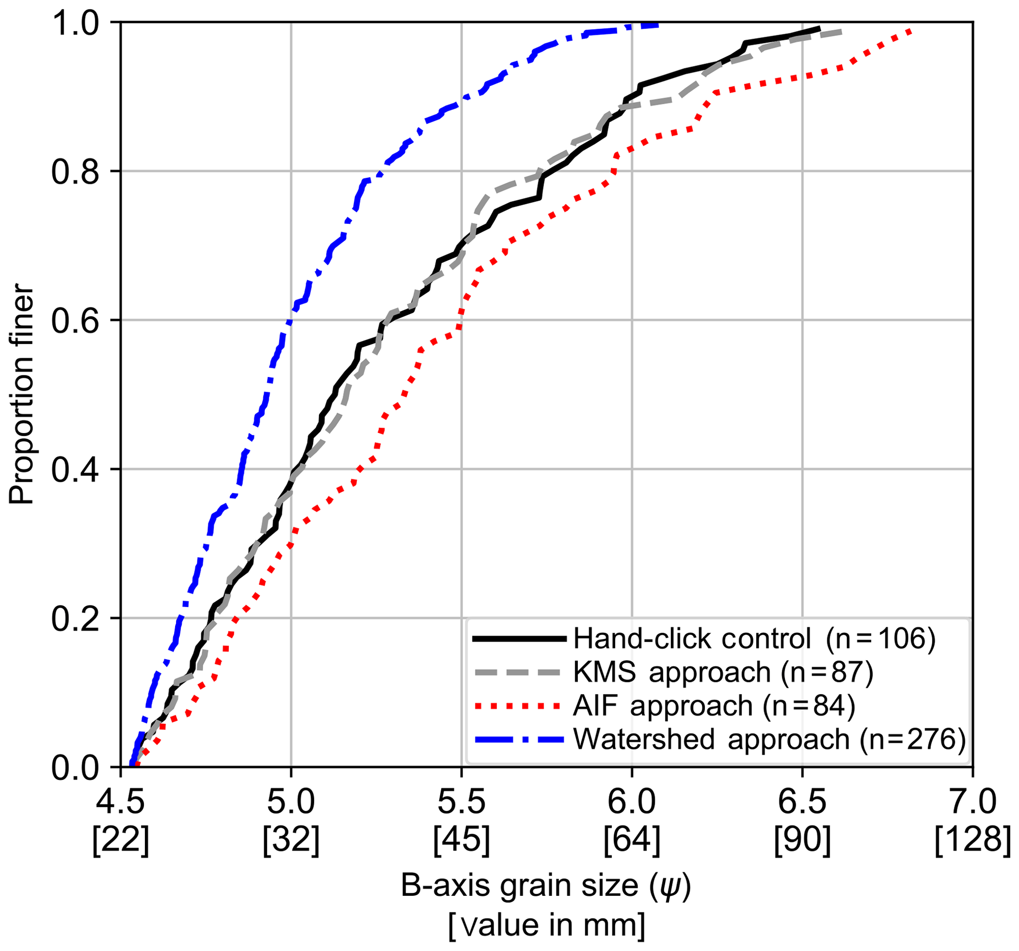
Figure 2Watershed segmentation (blue, dashed and dotted line) versus KMS (gray, dashed line) and AIF (red, dotted line) approaches compared with a hand-clicked b-axis grain-size distribution (black line) for a ∼1 m2 river patch (S09 in Fig. 6b). Watershed approach leads to oversegmentation of grains, giving an unreasonable number of clasts (276 versus 106 in the control) and an overly fine grain-size distribution.
Furthermore, faced with diverse camera models and the rise of SfM-MVS for the generation of georeferenced orthophotos, we wish to explore reasonable and appropriate combinations for covering acre-to-hectare areas while maintaining accurate grain-size measurement. Fundamentally, our aim for the KMS approach is not in the delineation of a single high-resolution image from a ∼1 m2 patch as in previous segmentation work but rather a method that can cover areas of 10–100 m2 containing complex grain arrangements, despite missing many grains at the patch scale. These semi-automated photo-sieving results can then be used to validate the AIF method at much greater spatial scales (102–104 m2), where physical counting is infeasible and previous methods are unreliable or time-consuming.
Our methods are similar to previous work by Graham et al. (2005a) and Detert and Weitbrecht (2012), with some key differences. A flow chart of both methods is shown in Fig. 3 and the processing is presented briefly. We direct the interested user to the manual (https://github.com/UP-RS-ESP/PebbleCounts) for a full description of the steps. Our algorithms use 2-D image processing in the spatial and spectral domains, which ignores the potential to exploit third height dimensions from irregularly spaced point clouds generated via lidar or SfM-MVS. The reader is directed to Sect. S1 in the Supplement for our efforts in this regard.
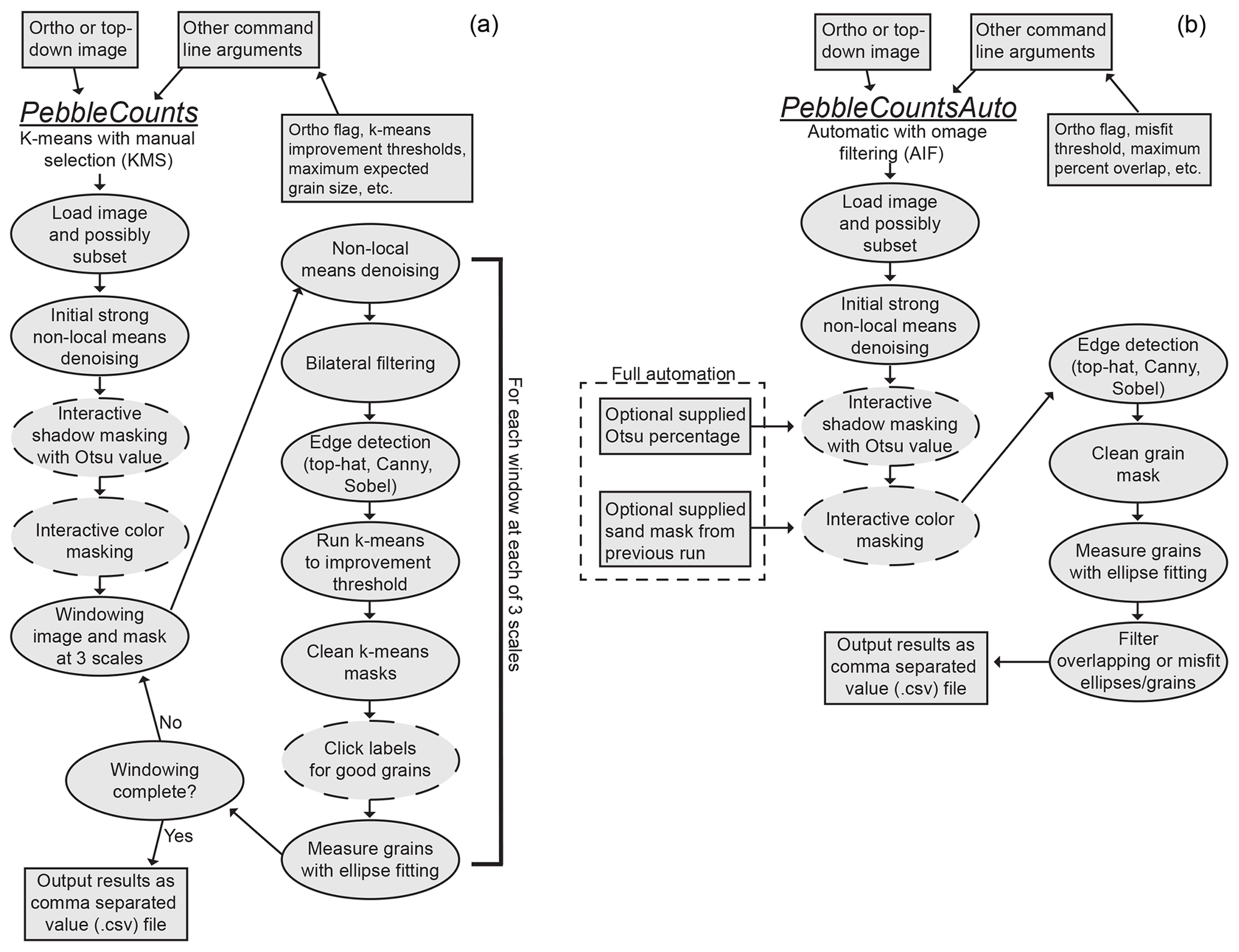
Figure 3Flowchart of PebbleCounts (a) and PebbleCountsAuto (b). The boxes are user-supplied input or output from the algorithm. Dashed lines indicate a user input step during processing, either entering and checking values or clicking.
2.1 PebbleCounts: KMS
We employ the additional color spaces HSV (hue, saturation, value) and CIELab (Russ, 2002), aside from traditional RGB (red, green, blue) and gray scale, to enhance differences in the spectral domain separate from lighting. First, the RGB image undergoes strong non-local means de-noising (Buades et al., 2011) to smooth intragranular color difference, interactive gray-scale shadow masking (Otsu, 1979) to separate obvious interstices, and HSV color selection for sand-patch masking (whereby sand is filtered by a narrow, user-selected color mask). The image and shadow/sand edge mask are then windowed for further processing.
At each window, the RGB image undergoes another weaker non-local means de-noising, is then converted to CIELab, and the chromaticity bands from this color space undergo bilateral filtering (Tomasi and Manduchi, 1998) to preserve intergranular edges while further smoothing color. Following this, edge detection on the smoothed, gray-scaled image occurs via a combination of top-hat, Sobel, and Canny methods with feature-AND selections (Russ, 2002), in which an edge is added to the full mask only if it overlaps with a found edge in the previous edge mask, thus piecewise building an edge map while avoiding lone (i.e., intragranular) edges (Detert and Weitbrecht, 2012).
After edge detection, our algorithm uses k-means clustering (Lloyd, 1982; Sculley, 2010) to further segment the pebbles. First, the matrix of non-masked pixels is converted into a vector that includes the spectral information at each location. This N×4-dimensional vector (N being the number of non-masked pixels) includes two spectral observables: the green–red and blue–yellow smoothed chromaticity bands from CIELab; and the two spatial observables: the x and y coordinates of the pixel in image space. To avoid oversegmentation by anisotropic or image-spanning grains, the x,y coordinates are rescaled to 50 % of the color, which is also rescaled from 0 to 1.
We attempted using agglomerative Ward hierarchical clustering (Ward, 1963) to further improve results on anisotropic and/or large grains; however, this approach is prohibitively slow on large images, and test results did not show significant improvement. The k-means clustering requires a user-supplied number of clusters. Here, we add clusters beginning at 1 and recalculate up to an inertia improvement threshold of 1 %–10 % (user supplied). Resulting labeled masks are cleaned via binary operations and the user is prompted to select the labeled regions that contain full, single grains within a simple pop-up window (Fig. S3).
After selection, the orientation and a and b axes of an ellipse fit to the labeled region, shown to accurately approximate grain size (Graham et al., 2005a), are recorded and the grain is added to the final list and the masked region. This processing takes place over three separate scales representing a “burrowing” of the algorithm through the image (from largest to smallest window/grain size). Scales are set by the user-supplied longest expected a axis and image resolution. In contrast to the 46 variables employed by Basegrain, PebbleCounts has 20 command-line variable flags – of which 15 exert influence on the results – with most requiring little to no modification (Table S1). Examples of the command-line interface and clicking steps are in the manual and Sect. S2.
2.2 PebbleCountsAuto: AIF
This method applies the same initial non-local means de-noising and interactive shadow/sand masking, with the option to input user-supplied values for full automation. From here, we diverge from the windowing and k-means approach and move directly to edge detection on the entire image using the same top-hat, Canny, and Sobel combination with feature-AND selections.
The resulting mask is then cleaned via binary morphological operations and each label is measured via ellipse fitting. To reduce the misidentified grains, the ellipses are filtered in a three-step chain. (A) Does the centroid fall within another ellipse? (B) Does the ellipse overlap with any neighboring ellipses above some threshold? (C) Is the percent misfit (ellipse area versus grain-mask area) above some threshold? At each step, an answer of “yes” leads to the elimination of the grain. The (A) and (B) steps filter grains that have high overlap or are oversegmented, whereas (C) helps filter areas where multiple grains were combined in one mask or a non-grain was identified (e.g., remaining sand patch). Grains passing the test are taken as the final results, with the assumption that misidentified grains are minimal, particularly when upscaling to large areas and tens of thousands of pebbles on high-quality (low-blur) images. The command-line variables for this method are shown in Table S2, and command-line examples can be found in the manual.
We experimented with resampling (over- and undersampling) the image prior to grain detection to increase smoothing and to improve the detection of larger grains at the cost of measuring fewer smaller grains. The majority of images achieved the best results using the original resolution, though we did find a slight improvement in results using undersampling on some unsharp images (see Sect. S3). The selection of other parameters like the maximum percent misfit is also covered in Sect. S3.
3.1 Experimental setup
To test the KMS and AIF approaches on a simple control, we arranged three distributions of well-rounded, river pebbles with a-axis sizes from 3 to 130 mm in semi-overlapping patterns in a 0.5 × 0.5 m area (Fig. 4). As opposed to most studies that use b-axis lengths to measure the grain-size distribution (Bunte and Abt, 2001), in the experimental setup, we use a axes since it was easier to hand-measure the longest axis of the >200 grains used. Six size-class bins (3–5, 10–20, 25–35, 40–50, 60–70, and 80–130 mm; all a axes) were sampled to approximate two log-normal and one bimodal grain-size distribution. The river pebbles used had uniform intragranular color with minimal striations (i.e., veins), low angularity, and a diverse array of intergranular colors. Lighting was controlled by overhead fluorescent bulbs and the photos were taken without flash to limit cast shadows.
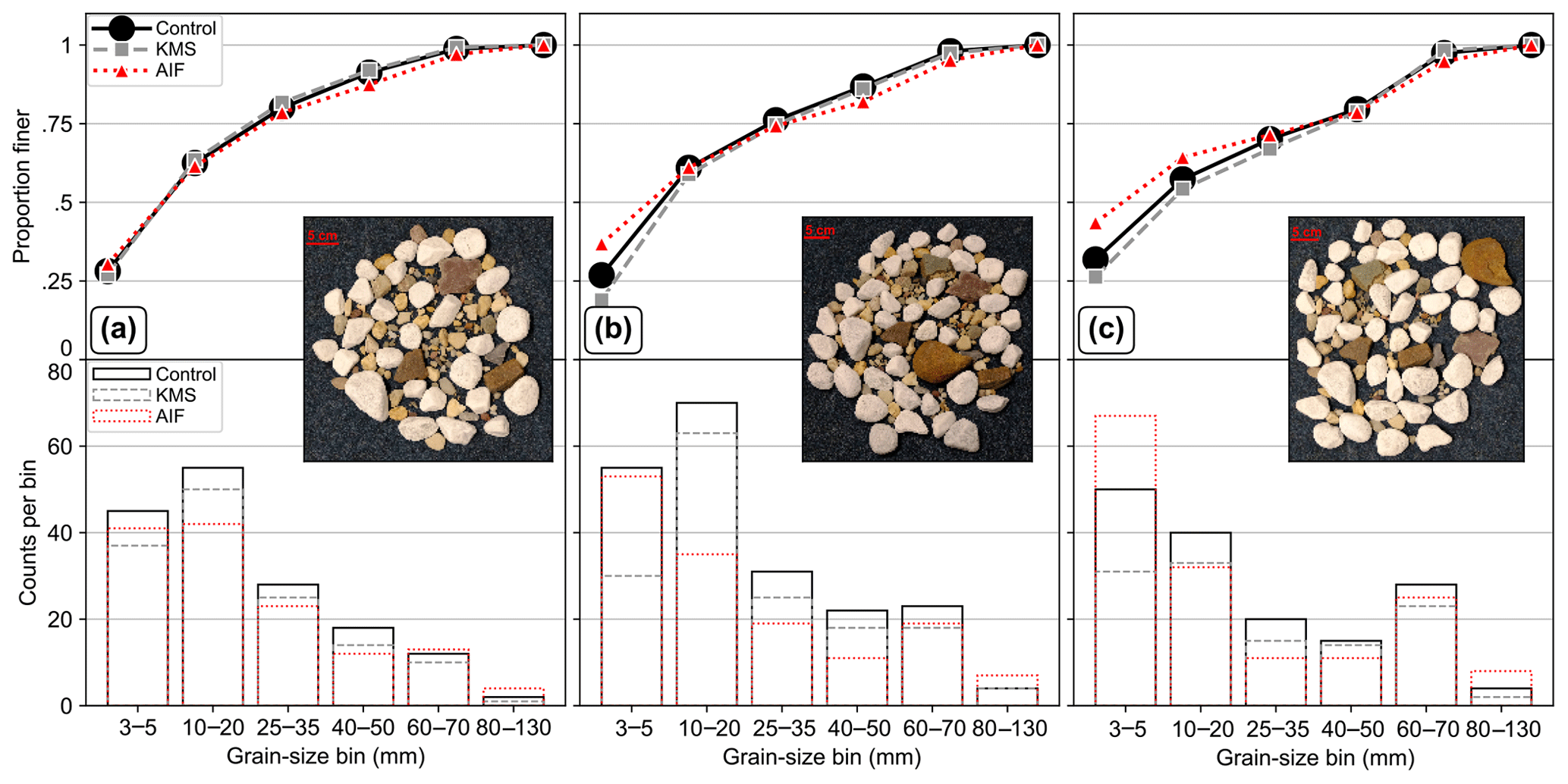
Figure 4Result of KMS (gray, dashed lines) and AIF (red, dotted lines) on the three experimental lab setups (a–c) with known grain inputs in six size classes (black line), measured as the grain a axis: (a) log normal, (b) log normal with increased number of all classes, including fines, and (c) skewed bimodal with increased number of coarser grains. Bottom row shows the counts per bin and the top row shows the resulting grain-size distribution. The images are 0.26 mm pixel−1 (24 megapixels).
3.2 Orthomosaic generation
We tested a Fujifilm X100F model camera with a fixed 23 mm focal length lens and a Sony α6000 model with a removable 35 mm fixed length lens. Both had the same advanced photo system type-C (APS-C) sensors (23.6 mm × 15.6 mm) and both output photos at 24 megapixels in a 4000 × 6000-pixel format. Following initial tests, it became clear that the image quality and grain-size results were practically identical for these two cameras, so the results presented are only those for the Fujifilm, as the photo quality was slightly sharper throughout and less distorted at the image corners. To simulate reduced quality, the 24-megapixel Fujifilm picture dimensions were reduced to 75 %, 50 %, and 25 %, resulting in 13.5-, 6-, and 1.5-megapixel images at pixel dimensions of 3000 × 4500, 2000 × 3000, and 1000 × 1500, respectively.
For each test setup, we collected ∼10 images from ∼20∘ off nadir (oblique) and at least four overhead near-nadir (tilts <10∘) pictures, for 12–16 photos in total. The collection of oblique images aided in removing doming effects from the resulting point clouds (e.g., James and Robson, 2014) and for capturing the pebble edges and sides (Fig. S1). As consumer-grade cameras have square pixels with negligible difference in horizontal and vertical resolution, the image scale can be calculated directly from the camera parameters and camera height with the resolution (R) in mm pixel−1 given by
where S is the sensor height or width in millimeters, f is the lens focal length in millimeters, h is the camera height in millimeters, and I is the image height or width in pixels. S and I should either both be the width or both be the height of the sensor and image, respectively. This assumes no major distortions within the field of view, which is not valid for oblique imagery but is negligible for near-nadir photography at close range using non-fisheye lenses. With h=1.55 m, the resulting image resolutions tested from the Fujifilm were 0.26, 0.35, 0.53, and 1.05 mm pixel−1 by Eq. (1).
We used the 12–16 photos to generate SfM-MVS orthoimages in Agisoft Photoscan v.1.4.2 (Agisoft, 2018) – renamed Agisoft Metashape in recent versions. This allows rapid output of additional information including point clouds, digital elevation models (DEMs), and the undistorted orthomosaics, with resolution recorded in the image metadata for direct input into PebbleCounts and PebbleCountsAuto. Detailed Agisoft processing steps are provided in Sect. S4.
3.3 Comparison metrics
For the simple controlled experiment, with relatively coarse grain-size bins, it is not appropriate to compare percentiles (e.g., D50) or to run Kolmogorov–Smirnov (KS) tests and measure the difference in distributions between the AIF or KMS and control grain-size distributions. Instead, we compared the counts in each bin between the control and algorithm and visually assessed the matching of the grain-size distributions. This provides a reasonable baseline for checking the performance of the algorithm in a highly controlled setting.
3.4 Results I: controlled experiment
For each of the three 150–200 clast arrangements, the KMS PebbleCounts runtime was ∼7 min on a laptop with 16 GB RAM and 2 cores (Intel i7-6650U 2.20 GHz) and no GPU, whereas the AIF PebbleCountsAuto runtime was ∼1 min. Both a single near-nadir image and the combined orthomosaic were used, but the results were entirely consistent aside from some inter-run variability in the KMS approach caused by the non-unique solution of k-means clustering. Given this consistency, we only present the results from the single near-nadir images. Furthermore, the use of only four overlapping near-nadir photos also generated the same results, albeit in about one-sixth the Agisoft orthomosaic processing time of using all 12–16 photos (∼10 min versus ∼1 h on the same laptop).
Across all three distributions, the KMS approach consistently undercounts the number of clasts in each a-axis bin (Fig. 4). However, and in agreement with previous research (Graham et al., 2010), this undercounting is uniformly distributed, and thus the grain-size distributions do not show notable differences between the algorithm and control. For the two arrangements with increased fine (3–5 mm) and coarse (60–130 mm) pebbles (Fig. 4b, c), the undercounting is stronger at the finer end of the distribution, leading to a slight underestimation of the grain-size distribution by the KMS approach in this region. This is caused partially by the user missing more of the smaller grains (of which there are exponentially more), some smaller grains being partially hidden by the larger, and also by the smallest grains being only a few pixels in area and thus eliminated during mask-cleaning steps or not captured at all. On the other hand, the AIF approach tends to overcount the fine pebbles, leading to overestimation of the grain-size distribution, because many small non-grain areas remaining in the masked image are automatically selected in the final result, rather than ignored as in the KMS approach.

Figure 5Results of reducing the image dimensions to (a) 75 % (13.5 megapixels), (b) 50 % (6 megapixels), and (c) 25 % (1.5 megapixels) and rerunning the KMS approach on the distribution in Fig. 4a. The control is shown as solid black (left y axis) and gray (right y axis) lines and KMS as the dashed lines.
As we reduced the resolution from 0.26 to 1.05 mm pixel−1, the reduction in the finest size class increased dramatically for the KMS approach (Fig. 5). At the lowest resolution tested (1.5 megapixels), this undercounting leads to severe discrepancies in the grain-size distribution curve. As the resolution degrades, it becomes more difficult to discern rocks in the smallest size class (3–5 mm), which correspond to a-axis grain sizes of 12–19, 9–14, 6–9, and 3–5 pixels for the 24-, 13.5-, 6-, and 1.5-megapixel resolutions, respectively, indicating the necessity of a limiting lower measurement factor (e.g., Graham et al., 2005a).
4.1 Field setting
Having established the algorithms on control data, we sought to evaluate the performance on complex, natural photos. Field data provide the real-world application and detailed uncertainty analysis most useful for researchers seeking to apply the methods to their own sites. For this, we turned to photo surveys carried out on gravel-bed river cross sections of the foreland and topographic transition zone of the northwestern Argentine Andes (Fig. 6). This is an area of strong precipitation, topographic, and environmental gradients, and the dynamic rivers surveyed are capable of transporting enormous quantities of sand, gravel, and boulders of various lithologies (Bookhagen and Strecker, 2012; Purinton and Bookhagen, 2018). Catchment-average erosion rates from the area, based on cosmogenic nuclide inventories, suggest rates on the order of 0.6–1 mm year−1 (Bookhagen and Strecker, 2012), with large variability during the Pleistocene and Holocene (Tofelde et al., 2017). The region is frequently affected by extreme hydrometeorological events that lead to flooding and drainage-pattern rearrangement (Castino et al., 2016, 2017).

Figure 6(a) Field cross-section survey sites (black triangles) in NW Argentina from three gravel-bed rivers (Toro, Vaqueros, and Grande) and their tributaries, draining from the sparsely vegetated mountains in the west towards the verdant foreland and city centers of Salta and Jujuy in the east. The Landsat 8 RGB composite satellite image (using bands 2, 3, and 4) from 12 June 2017 shows the climatic transition from wet foreland to dry mountains, demarcated by the green–brown transition zone, running approximately north–south, corresponding to vegetation changes. (b) Detailed view of the m2 orthomosaic clips from each of the field sites with average resolution of 1.16 mm pixel−1.
4.2 Orthomosaic generation
All cross-section surveys were collected using the Sony α6000 camera model at 24-megapixel resolution, and survey sizes ranged from ∼1000 to 5000 m2. In this case, the standard zoom lens delivered with the camera was used at the shortest focal length of 16 mm to maximize the field of view. Also, to help cover the large survey sites, the camera was affixed to the end of a pole with a remote control trigger, allowing overhead shots to be collected from a height of 4.5–5 m (Fig. 7), giving a ground resolution of approximately 1.1–1.2 mm pixel−1 by Eq. (1). UAV flights have proven difficult in the windy conditions experienced in these valleys, but flights at 20–30 m heights with the 12-megapixel camera provided on the DJI Mavic and Phantom models (focal lengths of 3.6–4.3 mm, sensor dimensions of 6.17 × 4.55 mm, and image dimensions of 4000 × 3000 pixels) would result in image resolutions of ∼7–13 mm pixel−1 and are thus inadequate for delineating centimeter-scale pebbles.

Figure 7Sony α6000 24-megapixel camera affixed to mast for photo collection at a height of 4.5–5 m (a) and differential GPS measurement of coded targets (b).
To generate georeferenced orthomosaics that could be tiled and passed directly to PebbleCounts and PebbleCountsAuto, survey sites on the dry riverbed were laid out with on average 18 coded targets (with a range of 10–24) and the position of each was measured with a differential GPS (Fig. 7). Kinematic post-processing with a permanent base station <100 km away at the Universidad Nacional de Salta (UNSA) in Salta, Argentina, led to centimeter accuracy of XYZ target locations. The site was traversed in a cross-hatched pattern with a photo captured every two to three paces, so that each location appeared in ∼9 near-nadir pictures from slightly different angles. We refer to the images as near nadir, rather than nadir, due to the fact that during mast photo collection some unintentional tilting of the camera (<10∘) occurred. These near-nadir photos aided in removing doming effects but did not allow us to capture the sides of pebbles as in the oblique images taken in the experimental setup (Fig. S1). Capturing oblique images of every patch in the field sites would require infeasible amounts of time and processing power.
Agisoft processing was similar to that described for the experiment, with some key differences (see Sect. S4). Given the volume of photos (600–1300 per site), the sites were processed automatically using the Python API for Agisoft, with processing times consistently over 10 h on an 80-core, 500 GB RAM server making use of 1 GPU NVIDIA Tesla K80 unit for some of the steps (e.g., dense matching).
From 10 of our full survey sites over three different river systems, we selected m2 patches to clip out of the full orthomosaics and evaluate using the KMS and AIF approaches. The final resolution of these 12 GeoTiff orthoimages matched the theoretical value from Eq. (1), with an average of 1.16 mm pixel−1 and range of 1.08–1.24 mm pixel−1 (standard deviation of 0.05 mm pixel−1). The patches (Fig. 6b) include variable amounts of sand and a large range of grain sizes, packing arrangements, and shadowing. From one site (S14A), there were handheld images available for the same selected patch from the same Sony α6000 camera zoomed to 20 mm focal length and taken from a height of ∼1.5 m, allowing for the generation of a complementary orthomosaic at 0.32 mm pixel−1 resolution.
4.3 Comparison metrics
For control data from the field, we return to b-axis measurements (rather than a axes as in the lab). In each patch, the b axes of all grains visible to the naked eye were manually digitized. This generated a 5490 pebble control dataset across all 12 mast-surveyed sites. For the lone handheld patch at 0.32 mm pixel−1, the control data were 1726 pebbles versus 621 from the same patch at the 1.12 mm pixel−1 mast resolution, as smaller grains could be manually measured on the image at a resolution that was 4 times greater.
The use of continuous control data, as opposed to discrete bins in the lab experiment, allows a more detailed investigation of the performance of both approaches, including biases and their correction. The b-axis measurements of overlapping control and KMS grains were compared to look for sizing bias. This was followed by a search for the lower truncation limit (the lower cutoff in b-axis length in pixels that grains are reliably measured at) of the algorithm, also using the KMS results. For parts of the analysis, the size data were converted to the typical ψ scale () of grain-size measurement of coarse river sediments. This allows direct comparison of statistical results with other studies (e.g., Graham et al., 2005b)
We compared the grain-size distributions from the KMS and AIF approaches with the control using a two-sample KS test to check the null hypothesis that the two samples are drawn from the same distribution. Because sample sizes were at times small, leading to erroneous KS-test results, we also devised a second metric of grain-size distribution comparison. Similar to the KS test, which uses the maximum distance between the cumulative distribution functions (grain-size distributions), our metric interpolates both distributions to the same lengths in 0.1 ψ steps and then sums the difference between the re-interpolated curve to give an approximate integral of the difference between the two grain-size distributions (AIF or KMS minus the control), which we term Adiff. Here, an Adiff value close to 0 indicates good matching, and positive or negative values indicate underestimation or overestimation, respectively.
We also examined the performance of some key percentiles (). The metrics for comparison of control (PC) and KMS or AIF (PP) percentiles are consistent with other studies (Sime and Ferguson, 2003; Graham et al., 2005b, 2010). These are the mean (), the mean squared (), and the irreducible random error (). The bias of PebbleCounts is quantified by m, and e measures the scatter or precision after bias correction (Sime and Ferguson, 2003).
4.4 Results II: field surveys
The KMS PebbleCounts approach took ∼10 min per 1 m2 orthomosaic clip at 1.16 mm pixel−1 resolution, depending on the number of grains, and particularly the number of finer grains, present. Runtime for the AIF PebbleCountsAuto approach was typically ∼2 min per site. All runtimes refer to the same laptop with 16 GB RAM and 2 cores (Intel i7-6650U 2.20 GHz) and no GPU. For the 0.32 mm pixel−1 image, the processing for KMS took ∼45 min, as there were more fine grains to be identified (given the log-normal distribution) and so the clicking took exponentially longer, and the AIF took ∼20 min given the longer time spent filtering the large number of grains. We note that the use of a GPU for the filtering steps will significantly improve processing time. Importantly, these runtimes refer to the use of no lower truncation value, which leads to much longer processing time.
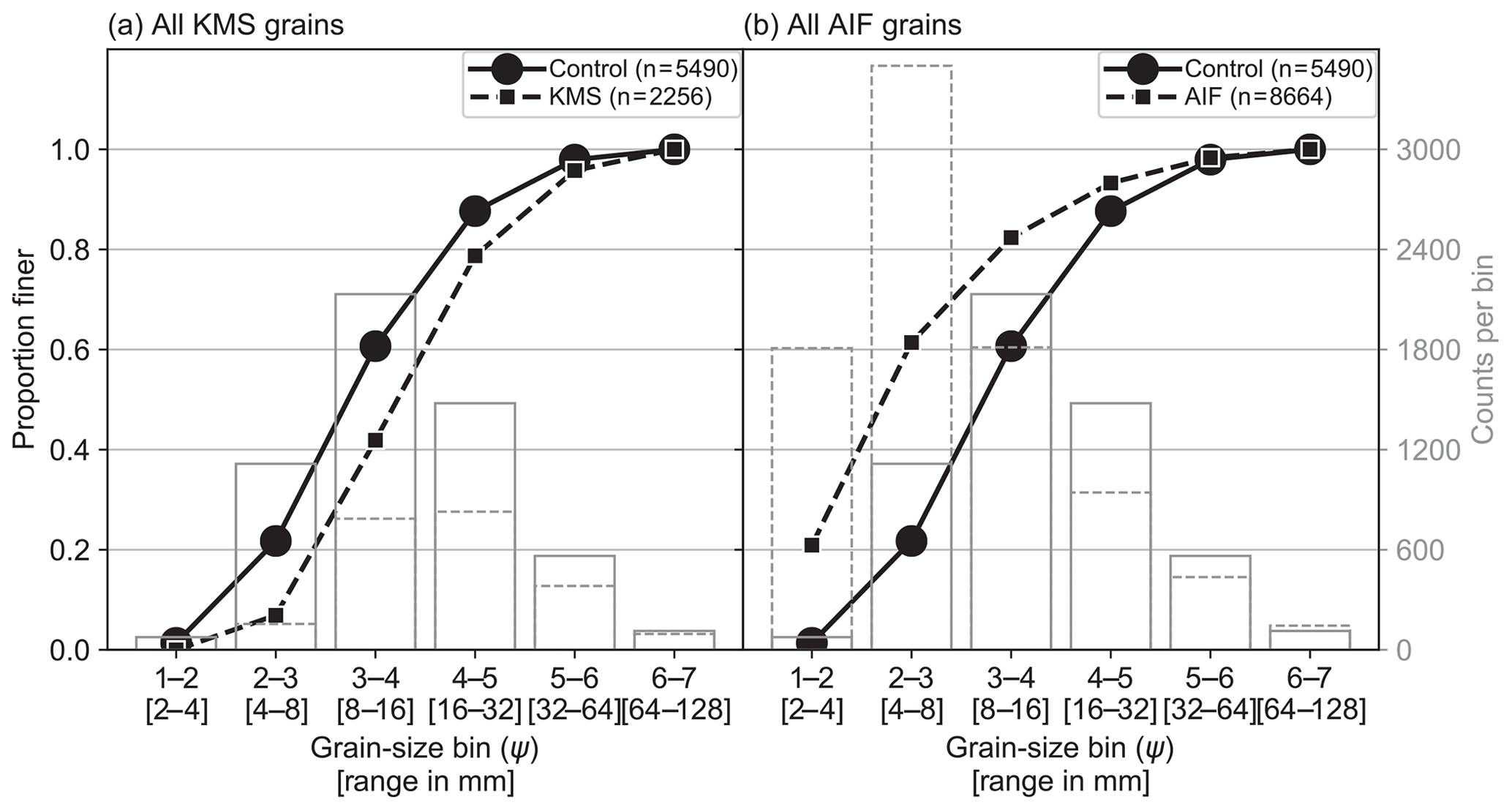
Figure 8Comparison of (a) KMS and (b) AIF at the 12 field sites all aggregated and coarsely binned. Control is shown as solid black (left y axis) and gray (right y axis) lines and KMS and AIF as the dashed lines.
An aggregation and coarse binning of all b axes in the control versus KMS and AIF data for the coarser imagery are presented in Fig. 8. There is obvious undercounting in these data from the KMS results, similar to the experimental setup, and here it causes a significant discrepancy in the grain-size distribution curves. Whereas the manual clicking found over 1000 grains in the smallest classes (1–2 and 2–3 ψ), the KMS approach found none in the smallest and only ∼100 in the second smallest. This skews the percentiles to the higher grain sizes and thus overestimates them significantly. In opposition to this, but again in agreement with the experimental setup, the AIF results display significant overcounting at the finer sizes as many non-grains are identified, particularly when the algorithm is run with no lower truncation.
The skewed results from both the KMS and AIF approaches warrant detailed analysis of the algorithms’ deficiencies and grain-size distribution corrections. To begin, we examined the performance of PebbleCounts on grains manually digitized and the same grains selected during clicking in the KMS approach on the coarser imagery (Fig. 9). There is only a slight negative bias across all grain sizes, indicating underestimation of individual grains by PebbleCounts; however, this median shift varies with no apparent pattern and is likely caused by uncertainties in the manual b-axis digitization of thousands of grains. For instance, digitization with b-axis vector lines can achieve subpixel accuracy compared to the raster processing of PebbleCounts. The AIF approach measures grains identically to the KMS method and thus has the same misfit errors on correctly identified grains. From this, we conclude that the algorithm is effective on a grain-by-grain basis and the skewing of the grain-size distributions is instead caused by sampling errors related to the image resolution and ability to find small grains (see Fig. 5).
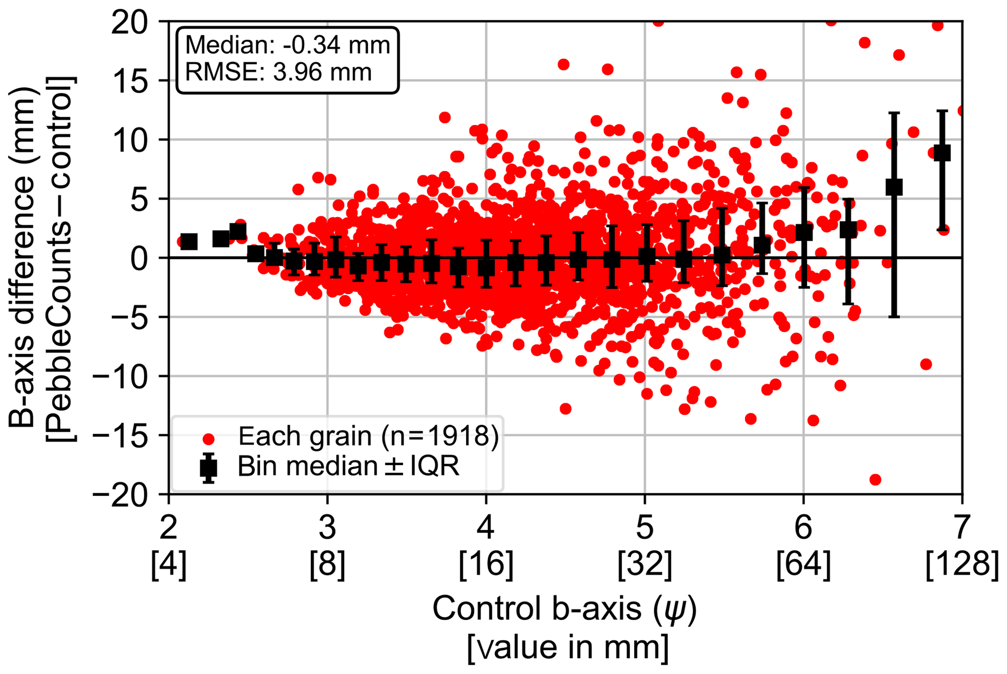
Figure 9Measurement error of PebbleCounts (here the KMS results) versus control on a grain-by-grain basis for overlapping grains in the coarser (1.16 mm pixel−1) imagery. There is an overall median shift, but the binned medians do not display a consistent pattern.
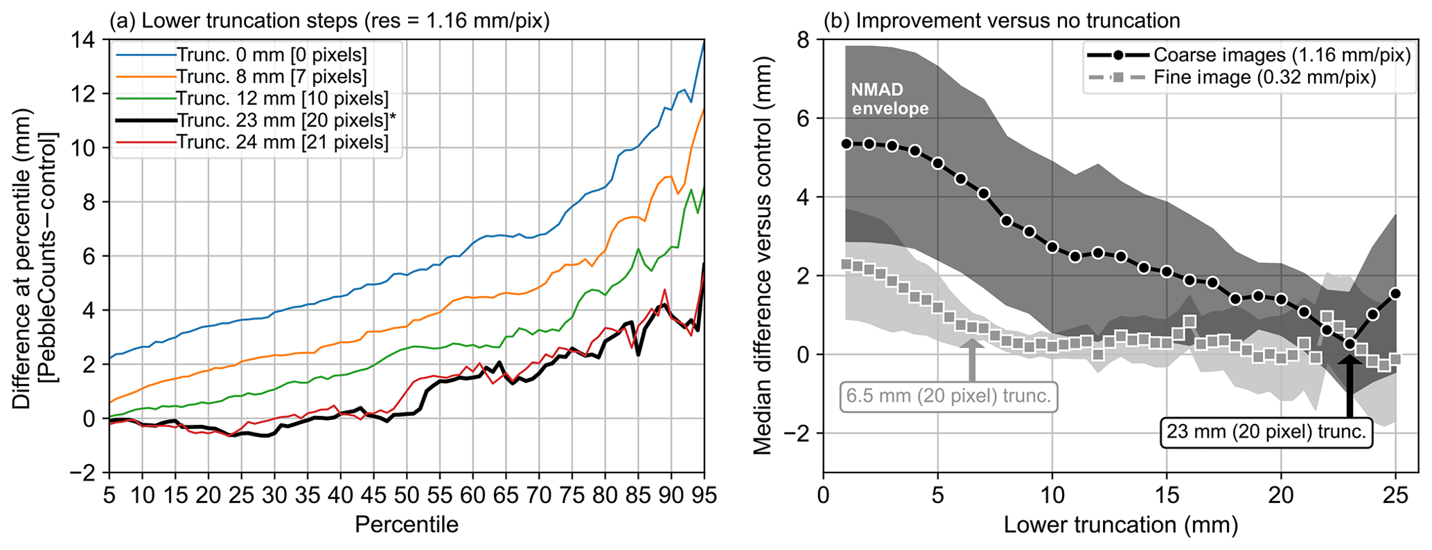
Figure 10(a) Error in each percentile (5th–95th) as lower truncation value is increased in 1 mm steps for the 1.16 mm pixel−1 imagery. Only a few steps are plotted for clarity. (b) The median difference in percentiles compared with the control versus the lower truncation value, with the normalized median absolute difference (NMAD) shown as the error envelope (Höhle and Höhle, 2009). From this analysis, we select a lower truncation of 20 pixels. The analysis in panel (a) was repeated for the finer image (with 0.5 mm truncation steps) to get the gray squares line in panel (b) and is not shown here.
The undercounting error can be explored on the full distribution of pebbles by gradually increasing the lower truncation value and assessing the error in percentiles versus the control data at each step (Fig. 10). As truncation is increased, the median percentile error decreases rapidly up to an inflecting value – manually chosen from the graph as a significant local minimum where the median difference is near 0 mm. Truncating the KMS distributions at a minimum b-axis length of 23 mm (rounded to 20 pixels) improves the results significantly for the 1.16 mm pixel−1 imagery taken from the mast. Beyond this truncation, there is limited improvement. Regarding the 0.32 mm pixel−1 image, the 20-pixel (6.5 mm) truncation also results in a median difference near 0 mm, with subsequent truncation values leading to only ∼0.5 mm improvements. Supplying these truncation values directly to the KMS PebbleCounts tool results in reduced processing time to ∼5 min for the coarser imagery and ∼15 min for the finer, as many small grains were then ignored and left out of the clicking mask.
The same analysis for the AIF approach is complicated by the large number of false grains found and the extreme overcounting of fine grains. Given this, we instead make the assumption that the similarity of the two methods, particularly in the edge detection and ellipse fitting steps, leads to similar errors in both. Therefore, we assume the same 20-pixel truncation. For the AIF PebbleCountsAuto tool, processing times with the 20-pixel truncation reduced to <1 min and ∼3 min for the coarse and fine images, respectively.
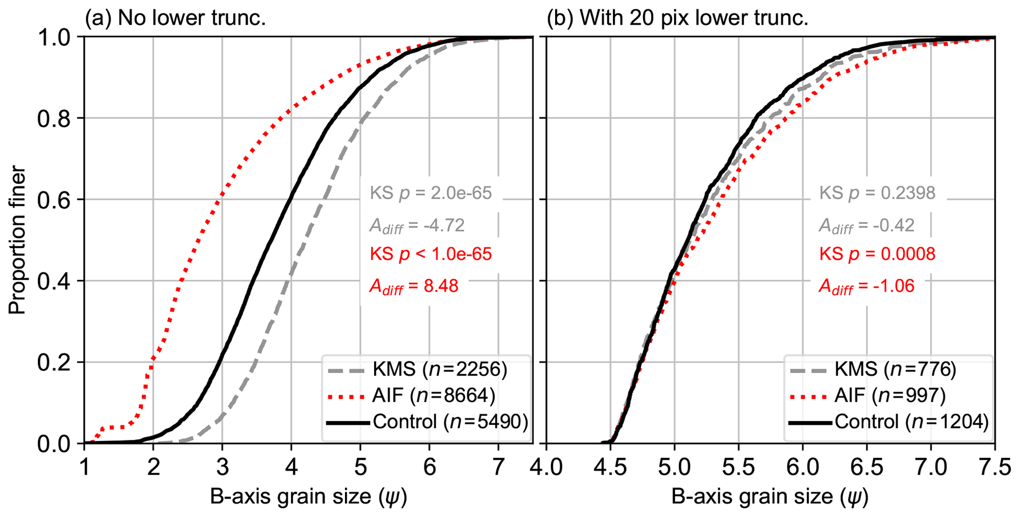
Figure 11Results from hand-clicked control (black line), KMS PebbleCounts (gray, dashed line), and AIF PebbleCountsAuto (red, dotted line) with the initial non-truncated run (a) and the 20-pixel truncated run (b). In corresponding colors are the p value results of a KS test and the Adiff approximate integral between the curves for each approach versus the control data. The legend indicates the number of grains (n) making up each curve. Note the reduction in x-axis scale between the columns, where the right truncated distributions are plotted on a narrower range to emphasize the remaining discrepancies. The curves separated by site (Fig. 6b) are shown in Sect. S5 and Fig. S7.
The combined results before and after lower truncation for the coarser (∼1.16 mm pixel−1) imagery taken from the mast surveys are shown in Fig. 11. Without any lower truncation, the AIF tool results in significant overcounting and grain-size distribution underestimation with a high Adiff>8. The KMS tool instead shows undercounting and grain-size distribution overestimation with a low . Both have KS-test p values <0.0001. When we apply a 20-pixel truncation, both the AIF and KMS approaches achieve Adiff values near or below −1, with the manual KMS approach performing best and achieving a high KS-test p value of 0.2398. The AIF approach retains a low p of 0.0008 with a ∼0.1–0.2 ψ bias towards coarser values in the upper portion of the grain-size distribution (>D50).
In Sect. S5 (Fig. S7), we show the 20-pixel truncated KMS and AIF results on a site-by-site basis. For the KMS approach, following truncation, 11 sites have p values >0.1 and one site (S16) has p=0.0971. Adiff values are also near 0, indicating close matching of the grain-size distributions, aside from S24 and S34, which both show large discrepancies. The AIF results in Fig. S7 follow a similar trend to the KMS results, but there is a bias towards coarser values, with many Adiff values , and generally poorer results compared with the KMS approach, with grain-size distributions being overestimated by ∼0.1–0.2 ψ. In the KMS results, despite a high p value, S24 demonstrates a stronger bias in the grain-size distribution towards coarser grains (up to 0.5 ψ discrepancy), as indicated by the high Adiff value of −1.36. Here, the KS-test pass is likely caused by the small sample size remaining after truncation (n=24), the least of any site. The poor performance of S24 was expected given the large size range with many sub-centimeter pebbles and a few large boulders, strong cast shadows from the large grains, and intragranular edges on angular boulders with quartz veins (see Fig. 6b). Importantly, S24 is the only site not from a major river stem but rather from a debris-flow fan draining a small tributary catchment in the Quebrada del Toro. S34 also had a high . In this case, poor performance is due to significant blurriness of this image and again a small sample size (n=47).

Figure 12Comparing the key b-axis percentiles across all 12 field sites and between the KMS and AIF approaches with the 20-pixel truncation applied. (a) All 12 sites from KMS, (b) KMS improvement when excluding S24 and S34, (c) all 12 sites from AIF, and (d) AIF improvement when excluding S10, S24, and S34. For the main plot, each data point is a percentile value from a single site and the 1 : 1 relationship is the gray diagonal. The mean (m), mean squared (ms), and irreducible (e) errors are shown for each plot, taken as the average of all seven percentile errors across the 9–12 sites plotted. The m and e are separately plotted for each percentile in the inset plot. The number of grains in the control (“control grains”) and KMS or AIF results (“grains found”) is also indicated. The individual site curves where these data points originate are shown in Sect. S5 and Fig. S7.
We also compared the individual percentiles of interest to assess the bias and accuracy of truncated results (Fig. 12). For the KMS approach, the bias (m) is 0.06 ψ with a precision (e) of 0.13 ψ. Excluding S24 and S34, m and e drop to 0.03 and 0.09 ψ, respectively. The AIF results have higher m and e values of 0.15 and 0.17 ψ, respectively, which are reduced to 0.13 and 0.15 ψ following exclusion of the same S24 and S34 sites, in addition to the S10 site, which was also somewhat blurry and with relatively few grains. For the AIF percentiles, we chose to include S16 despite a large overestimation at higher percentiles (Fig. S7), as this was a sharp image with a relatively large sample size. The high uncertainties from this scene likely require some adjustment of the edge-detection variables (see Sect. S3) for improved segmentation, but the results presented are realistic for fast processing using the AIF method, with the caveat of higher expected uncertainties.
The uncertainties in Fig. 12 are average values, and the inset plots also demonstrate the increasing uncertainty of larger percentiles. The maximum uncertainty for both at D95 is m=0.08ψ and e=0.07 ψ for the KMS result and m=0.35ψ and e=0.2ψ for the AIF result. Importantly, since the ψ scale is logarithmic, the larger errors at higher percentiles correspond to similar percentage misfits as lower errors at smaller percentiles (e.g., 0.2 ψ precision at a grain size of 6.5 ψ (91 mm) is a 13 %–15 % misfit, whereas a 0.01 ψ precision at 4.5 ψ (23 mm) is a 4 %–10 % misfit).
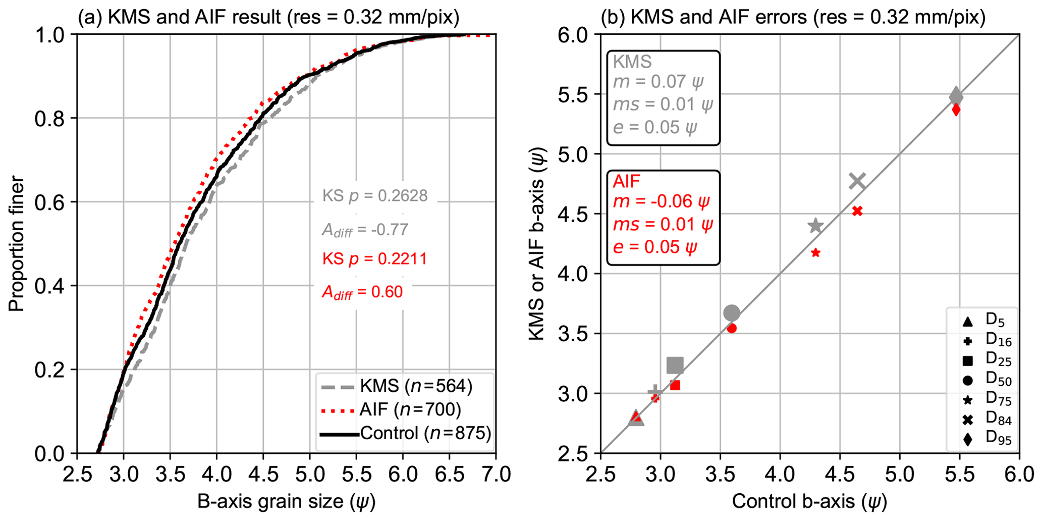
Figure 13(a) Results from hand-clicked control (black line), KMS PebbleCounts (gray, dashed line), and AIF PebbleCountsAuto (red, dotted line) from the 20-pixel truncated run on the 0.32 mm pixel−1 handheld imagery. In corresponding colors are the p-value results of a KS test and the Adiff approximate integral between the curves for each approach versus the control data. (b) Percentile comparison for both methods with KMS in gray and AIF in red, with inset box showing the uncertainties for each in the corresponding color.
As a final test for the KMS and AIF approaches, we turn towards our handheld imagery taken from S14A with a 4 times greater resolution of 0.32 mm pixel−1 (Fig. 13). We only show the 20-pixel truncated results, which displayed high KS-test p values >0.2 and Adiff close to 0 in both cases, with the AIF approach slightly underestimating (Adiff=0.6) and KMS slightly overestimating (). For the KMS approach, m and e are 0.07 and 0.05 ψ, respectively, and −0.06 and 0.05 ψ for AIF.
4.5 Caveat of PebbleCountsAuto AIF
The promising results of the AIF approach shown in Figs. 11–13 come with some consideration of the grain-by-grain accuracy. In Fig. 14, we analyze the percentage of grains found in the AIF approach that have a corresponding grain in either the hand-clicked control (based on a 6 mm buffer of the b-axis line) or the KMS results (based on a 6 mm centroid buffer). From this subset of grains, we consider the AIF grain to be a matching (or correct) result if the b-axis difference between it and the nearby “good” grain (from the control or KMS) is <1 cm. From this, we see that in the best-case scenario the percentage of correct grains identified by the AIF approach is only 70 %, from the handheld 0.32 mm pixel−1 image. A number of sites (S10, S16, S20B, S24, S34, and S35) have <50 % matched grains. The two poorly performing sites (S24 with grain complexity and S34 with image blur) both demonstrate the lowest accuracy with <40 % matches. Notably, despite a significant number of false positives in the results, when comparing the overall grain-size distributions (Fig. 11), and on a site-by-site basis (Fig. S7), the distribution of the AIF results matches the hand-clicked control well. The errors associated with the AIF method are demonstrated in Sect. S6.
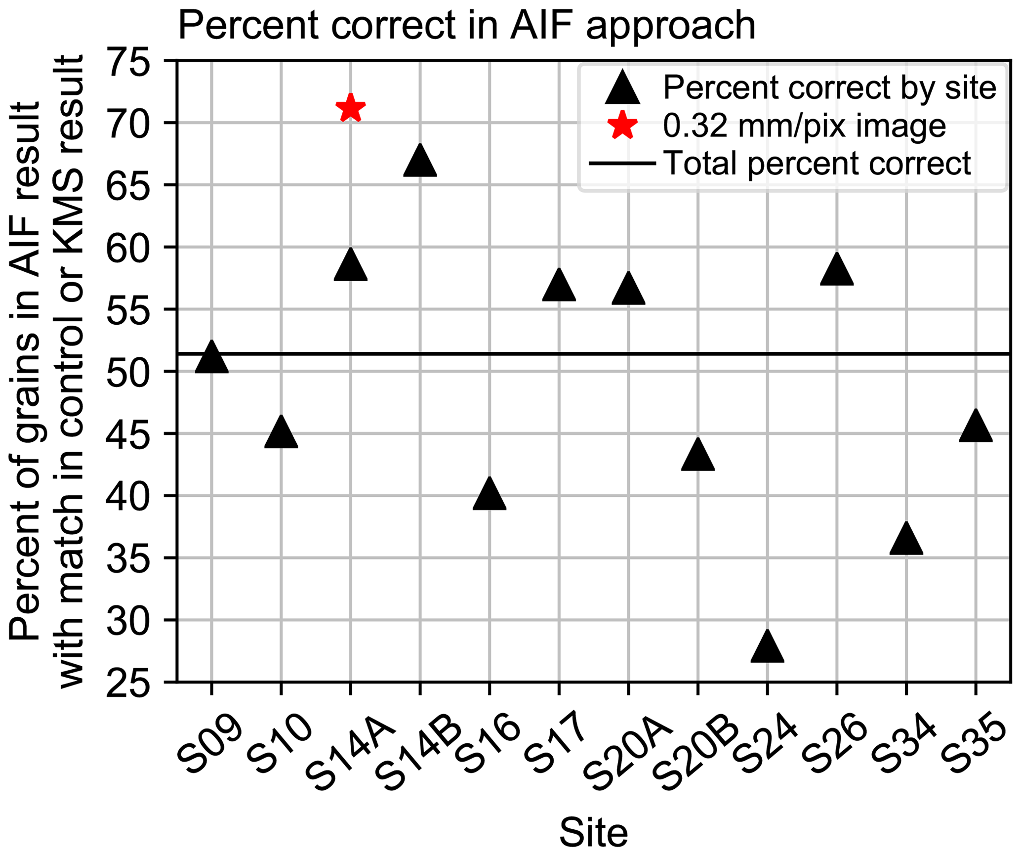
Figure 14Percentage of grains from AIF results with a matching grain in either the hand-clicked control or in the KMS result. A match is defined as a grain within 5 pixels of the hand-clicked line or the KMS grain centroid for the 1.16 mm pixel−1 imagery or within 20 pixels for the 0.32 mm pixel−1 image (corresponding in both cases to a distance of ∼6 mm), and with a 1 cm maximum b-axis difference between the AIF grain and the match. The total percent correct, taken across all black triangles, is 51 %.
In this study, we developed two new methods for grain-size measurement with low uncertainties and the potential to deliver full grain-size distributions from complex images of high-energy mountain rivers. Our open-source Python-based algorithms perform equally well to other image segmentation tools but can be applied more quickly over larger areas surveyed by the SfM-MVS workflow we present. Critical to success is the application of a strict lower cutoff, which limits the minimum measurable b-axis grain size to 20 times the pixel resolution. The automated version of the algorithm delivers less accurate measurements, but these can be limited by using low-blur, higher-resolution imagery. We focus our discussion on the comparison of our approach with similar work, the effect of the lower truncation on grain-size distribution estimates, and practical guidelines for acquiring imagery and applying PebbleCounts, including the application of UAV surveys.
5.1 Performance
For comparison of our algorithms to previous work, we do not consider errors reported in studies using texture-based measurements (e.g., Woodget et al., 2018), since these are based on correlative relationships rather than physical measurement of each grain. Texture methods work well for homogeneous pebble arrangements in lower-energy settings, but high-energy mountain rivers with heterogeneous pebble arrangements and large ranges in sizes require segmentation approaches. Similar to other image segmentation methods, the KMS PebbleCounts approach undercounts grain sizes in each respective size class (Graham et al., 2010). This undercounting does not undermine the resulting grain-size distributions and associated percentile estimates, so long as an appropriate lower truncation is defined. This cutoff was found to be 20 pixels (compare to 23 pixels found by Graham et al. (2005a)) in b-axis length (Fig. 10), which explains the degradation in 3–5 mm counting in the reduced-resolution lab images (Fig. 5), where the smallest pebbles were only a few pixels in size as resolution was decreased.
As shown in Fig. 12, when we apply this cutoff and exclude poorly performing images, we find an average m (bias) and e (precision) of 0.03 and 0.09 ψ, respectively, for the ∼1.16 mm pixel−1 imagery and 0.07 and 0.05 ψ for the 0.32 mm pixel−1 image. For the AIF approach, these values are 0.13 and 0.15 ψ for the ∼1.16 mm pixel−1 imagery and −0.06 and 0.05 ψ for the 0.32 mm pixel−1 image. These are averages, which actually increase at higher percentiles in agreement with other image segmentation methods (e.g., Sime and Ferguson, 2003). We thus suggest higher error budgets at higher percentiles.
As demonstrated in Figs. 14 and S8, there are significant inaccuracies associated with the AIF approach. The errors associated with the AIF approach can be limited when applied to high-quality (low-blur) ∼1 mm pixel−1 resolution imagery, with better results possible on <0.5 mm pixel−1 imagery. Ultimately, the uncertainties are highly dependent on the input image quality and complexity (range in grain size, angularity, intragranular variability) and providing blanket estimates is less useful than end users applying the KMS tool to a subset of images to validate the results of the AIF approach.
Butler et al. (2001)Sime and Ferguson (2003)Graham et al. (2005b)Westoby et al. (2015)(Detert and Weitbrecht, 2012)Table 1Comparison of PebbleCounts and PebbleCountsAuto results with other segmentation-based pebble counting studies.
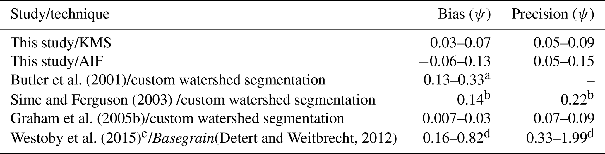
a Taken from only three percentiles (). b Corrected value presented by Graham et al. (2005b). c Comparison made in millimeters, converted to ψ units here. d Large spread caused by significant disagreement at higher percentiles.
In spite of this caveat, our bias and precision values of −0.06–0.15 ψ are on the low end of previously published errors from similar techniques (Table 1). To our knowledge, the only study to compare Basegrain results to control data by Westoby et al. (2015), makes comparisons in millimeters rather than ψ units. Since the ψ scale is logarithmic, in our study, the error in millimeter increases with ψ from ∼0.8 mm uncertainty at 4.5 ψ (23 mm) to ∼7 mm uncertainty at 6.5 ψ (91 mm) for the ∼1.16 mm pixel−1 imagery in the KMS case. Westoby et al. (2015) report even greater bias and lower precision from Basegrain, with errors also increasing in magnitude at higher percentiles. We emphasize that the previous image segmentation techniques discussed all rely on watershed segmentation, whereas neither of our algorithms use this step for the reasons demonstrated in Figs. 1 and 2.
5.2 Lower truncation
The issue of lower truncation on grain-size distributions and percentile estimates has received much attention in the literature (e.g., Fripp and Diplas, 1993; Rice and Church, 1996; Bunte and Abt, 2001; Graham et al., 2010). Previously, field geomorphologists were interested in all grains above 8–16 mm, simply because smaller grains were difficult to manually identify and thus underrepresented in the results (e.g., Fripp and Diplas, 1993; Rice and Church, 1998). Previous work suggests that truncation at the finer end of the distribution primarily increases the lower percentiles, while having less effect on the large (>D50) percentiles (Bunte and Abt, 2001). We find significant shifts in all percentiles of >0.5 ψ when applying a 20-pixel truncation. Graham et al. (2010) report truncation errors of <0.3 ψ for all percentiles in 1, 3, and 5 ψ truncated distributions. Their better results at lower percentiles are likely because the data were collected manually grid-by-number style in the field with the ability to include smaller grain sizes. The measurement resolution presents the ultimate control on how accurately grain-size percentiles can be measured. The purpose of the KMS and AIF approaches introduced here is in acquiring grain-size distributions from a subset of the full grain-size range present in the river, namely the subset with >20-pixel b-axis length in image resolution.
5.3 Image acquisition
Ideally, collecting more than nine near-nadir images m−2 (as in our field surveys) or collecting an approximately 1 : 2 (or greater) ratio of near-nadir to oblique imagery (as in our experiments with point-cloud data dimensions; see Sect. S1), leads to the highest quality point-cloud results in Agisoft. Higher-quality point clouds, in turn, lead to less distortion errors during orthorectification and higher-quality orthomosaics. Due to the textured nature of gravel images, we attained comparable results in reduced time using only four overlapping near-nadir images m−2 in the lab setting. In any case, high overlap of ∼80 % between images is recommended to ensure the best results. Where a user desires accurate and dense point-cloud data in addition to the 2-D orthomosaics, it is recommended that (many) more images closer to the surface be collected (e.g., Verma and Bourke, 2019) and from oblique viewing angles (e.g., James and Robson, 2014).
As we find the difference in calculated resolution and subsequent grain-size measurement to be negligible between orthorectified and raw near-nadir imagery at these scales, the use of orthoimagery is not strictly necessary when using image-segmentation software like PebbleCounts (e.g., Carbonneau et al., 2018). However, on very rough surfaces with cast shadows from large grains, generating orthoimagery will overcome distortions present in the raw photos. Furthermore, georeferenced orthomosaics may be preferable for capturing large sites at a constant resolution that can be fed into the algorithm.
In terms of camera and photographic height (and thus resolution) considerations, one first needs to assess the minimum grain size that is desired. Following this, the resolution of the image can be determined using Eq. (1) with some knowledge of the camera parameters (focal length, camera height, sensor size, and image size). The smallest grain b axis needed should be 20 times this resolution. For instance, using a similar camera to the Sony α6000 (24-megapixel, 15.6 × 23.5 mm sensor, 16 mm focal length), to measure all grains down to 1 cm one needs a resolution of 0.5 mm pixel−1 and thus a maximum camera height of ∼2 m. If finer grain sizes are desired, the user can use higher-resolution imagery but must be aware of the longer time needed for processing.
5.4 UAV surveying
The >20 m flight heights typical of UAV surveys lead to centimeter-scale imagery with currently available 12- to 24-megapixel cameras, which is less appropriate for PebbleCounts processing, unless large (>0.2 m) cobbles and boulders dominate the river site. Acquiring 0.5 mm pixel−1 imagery from a DJI Mavic drone with a 12-megapixel camera requires a very low flight height of ∼1.4 m, giving a field of view of only ∼ 1.5×2 m. This may be improved using better cameras like on the Mavic 2 Pro (20-megapixel camera), but gathering such imagery with the high overlap (∼80 %) required for SfM-MVS processing is still difficult, particularly given current ∼20 min flight length limitations from available batteries. Given continual technology improvements (e.g., greater battery life, more accurate geotags from onboard dGPS, higher megapixel cameras, and reduced motion blur), it is within reason to expect hectare to multi-hectare SfM-MVS UAV surveys at mm resolution in seamless orthomosaics along entire river reaches in the near future. But, for the time being, a single, non-overlapping orthoimage workflow proposed by Carbonneau et al. (2018) has high potential to achieve large-areal results. Their workflow, building on Carbonneau and Dietrich (2017), uses a number of high and oblique overlapping flights to orthorectify a lower non-overlapping flight with millimeter-scale acquisition, with resulting single, scaled images passed to Basegrain, or, alternatively, to PebbleCounts.
5.5 Coverage and processing limits
Using handheld imagery, a survey site of 1000–5000 m2 with ∼10 ground control points (GCPs) measured via dGPS can be covered in 2–6 h by one person (including GCP collection). Using a camera-on-mast setup, this time can be reduced by half, with even greater speed possible using more people and cameras (of the same sensor dimensions, focal length, and height). The potential to cover even larger sites up to or exceeding 100 × 100 m (1 ha) is feasible in a day of work by two people (with one measuring the targets and both sharing the photo-taking) using the proposed method with a 16–20 mm focal length lens and a 3–5 m mast.
One limit of the scalability of the PebbleCounts method is processing time. The KMS PebbleCounts tool is recommended to be applied to maximum 1–2 m2 patches, depending on the image resolution, as the manual clicking of good grains is time-consuming, requiring 5–20 min per patch depending on patch size, image resolution, and abundance of finer grains. On the other hand, the AIF PebbleCountsAuto tool can theoretically be applied at larger scales. However, it is also advisable to tile data and feed them to the algorithm in maximum 1–2 m2 patches for ∼1 mm pixel−1 imagery, since the non-local means de-noising can take minutes on very large images ( pixels). Again, the use of systems with GPUs or large memory will shorten processing times and allow for larger images to be run.
In practical terms, a workflow to cover a ∼2500 m2 survey site captured at 1 mm pixel−1 resolution and processed into a georeferenced orthomosaic would be (1) tiling into 2 m2 patches, (2) passing each patch to the AIF PebbleCountsAuto tool with quick manual steps of shadow-masking and sand-clicking (if sand is present), where each tile takes 1–2 min, (3) selecting a random subset of ∼20 tiles to pass to the KMS PebbleCounts tool as validation and uncertainty estimation for the AIF approach. Such a workflow could be accomplished in 1–2 d of work by an experienced user, providing tens to hundreds of thousands of measured grains from the survey site and a robust measurement of the full grain-size distribution. To increase processing speed, a gridded subset of tiles could also be extracted from the full survey site, with a 3–5 m step size between patches, to provide complete coverage across heterogeneous gravel-bar features, while avoiding unnecessary oversampling and processing of every patch in the survey site.
Using a k-means approach for pebble segmentation in the spectral and spatial domain combined with fast manual selection of good results, we developed a new semi-automated algorithm for grain sizing optimized for images taken over gravel-bed rivers (PebbleCounts). We also developed an automated algorithm that uses suspect grain filtering (PebbleCountsAuto), albeit with larger uncertainties in the results. The lower truncation of the methods (minimum b-axis length measurable) is limited to 20 pixels and above. These new methods were necessary to acquire grain-size distributions from dynamic high-mountain rivers with complexity from sources such as large ranges in grain size, intragranular heterogeneity, grain overlap, irregular shadowing, and sand patches. Similar to previous methods, PebbleCounts is best applied at the patch scale (∼1 m2); however, PebbleCounts provides more realistic results in complex images without any post-processing steps in ∼5–10 min per patch, assuming ∼1 mm pixel−1 resolution imagery. PebbleCountsAuto performs very well on high-quality (low-blur) imagery, though with remaining misidentification that must be approached with caution. Grain-sizing results can be upscaled to areas on the order of 102–104 m2 when PebbleCounts results are used as validation for the automated PebbleCountsAuto function.
PebbleCounts is a Python-based program with the code and documentation available on GitHub at https://github.com/UP-RS-ESP/PebbleCounts (last access: 12 September 2019) (Purinton and Bookhagen, 2019).
The supplement related to this article is available online at: https://doi.org/10.5194/esurf-7-859-2019-supplement.
BB and BP defined the project. BP developed the algorithms with support from BB. BP carried out the analysis, produced the figures, and wrote the manuscript. BB provided funding, guidance in data analysis, and manuscript edits.
The authors declare that they have no conflict of interest.
Anna Rosner is thanked for assistance with fieldwork for mast surveys, and Steffen Wellegehausen is thanked for aiding in the lab experiment setup. Constructive reviews from Patrice Carbonneau, Pascal Allemand, and Eric Lajeunesse improved the structure of the manuscript.
This research has been supported by the DFG (IRTG-StRATEGy (grant no. IGK2018)) and the MWFK Brandenburg (NEXUS). We acknowledge the support of the open-access publishing fund of the University of Potsdam.
This paper was edited by Eric Lajeunesse and reviewed by Patrice Carbonneau and Pascal Allemand.
Agisoft: AgiSoft PhotoScan Professional, available at: http://www.agisoft.com/downloads/installer/ (last access: 12 September 2019), 2018. a
Attal, M. and Lavé, J.: Changes of bedload characteristics along the Marsyandi River (central Nepal): Implications for understanding hillslope sediment supply, sediment load evolution along fluvial networks, and denudation in active orogenic belts, Geol. S. Am. S., 398, 143–171, https://doi.org/10.1130/2006.2398(09), 2006. a
Attal, M., Mudd, S. M., Hurst, M. D., Weinman, B., Yoo, K., and Naylor, M.: Impact of change in erosion rate and landscape steepness on hillslope and fluvial sediments grain size in the Feather River basin (Sierra Nevada, California), Earth Surf. Dynam., 3, 201–222, https://doi.org/10.5194/esurf-3-201-2015, 2015. a
Bertin, S. and Friedrich, H.: Field application of close-range digital photogrammetry (CRDP) for grain-scale fluvial morphology studies, Earth Surf. Proc. Land., 41, 1358–1369, https://doi.org/10.1002/esp.3906, 2016. a, b
Bertin, S., Groom, J., and Friedrich, H.: Isolating roughness scales of gravel-bed patches, Water Resour. Res., 53, 6841–6856, https://doi.org/10.1002/2016WR020205, 2017. a
Bookhagen, B. and Strecker, M. R.: Spatiotemporal trends in erosion rates across a pronounced rainfall gradient: Examples from the southern Central Andes, Earth Planet. Sc. Lett., 327–328, 97–110, https://doi.org/10.1016/j.epsl.2012.02.005, 2012. a, b
Brasington, J., Vericat, D., and Rychkov, I.: Modeling river bed morphology, roughness, and surface sedimentology using high resolution terrestrial laser scanning, Water Resour. Res., 48, W11519, https://doi.org/10.1029/2012WR012223, 2012. a
Buades, A., Coll, B., and Morel, J.-M.: Non-Local Means Denoising, Image Processing On Line, 1, 208–212, https://doi.org/10.5201/ipol.2011.bcm_nlm, 2011. a
Bunte, K. and Abt, S. T.: Sampling surface and subsurface particle-size distributions in wadable gravel- and cobble-bed streams for analyses in sediment transport, hydraulics and streambed monitoring, Tech. rep., US Forest Service, Rocky Mountain Research Station, Fort Collins, CO, https://doi.org/10.2737/RMRS-GTR-74, 2001. a, b, c, d
Buscombe, D.: Transferable wavelet method for grain-size distribution from images of sediment surfaces and thin sections, and other natural granular patterns, Sedimentology, 60, 1709–1732, https://doi.org/10.1111/sed.12049, 2013. a
Buscombe, D., Rubin, D. M., and Warrick, J. A.: A universal approximation of grain size from images of noncohesive sediment, J. Geophys. Res.-Earth, 115, F02015, https://doi.org/10.1029/2009JF001477, 2010. a
Butler, J. B., Lane, S. N., and Chandler, J. H.: Automated extraction of grain-size data from gravel surfaces using digital image processing, J. Hydraul. Res., 39, 519–529, https://doi.org/10.1080/00221686.2001.9628276, 2001. a, b
Carbonneau, P. E.: The threshold effect of image resolution on image-based automated grain size mapping in fluvial environments, Earth Surf. Proc. Land., 30, 1687–1693, https://doi.org/10.1002/esp.1288, 2005. a, b
Carbonneau, P. E. and Dietrich, J. T.: Cost-effective non-metric photogrammetry from consumer-grade sUAS: implications for direct georeferencing of structure from motion photogrammetry, Earth Surf. Proc. Land., 42, 473–486, https://doi.org/10.1002/esp.4012, 2017. a
Carbonneau, P. E., Lane, S. N., and Bergeron, N. E.: Cost-effective non-metric close-range digital photogrammetry and its application to a study of coarse gravel river beds, Int. J. Remote Sens., 24, 2837–2854, https://doi.org/10.1080/01431160110108364, 2003. a
Carbonneau, P. E., Lane, S. N., and Bergeron, N. E.: Catchment-scale mapping of surface grain size in gravel bed rivers using airborne digital imagery, Water Resour. Res., 40, W07202, https://doi.org/10.1029/2003WR002759, 2004. a, b
Carbonneau, P. E., Bizzi, S., and Marchetti, G.: Robotic photosieving from low-cost multirotor sUAS: a proof-of-concept, Earth Surf. Proc. Land., 43, 1160–1166, https://doi.org/10.1002/esp.4298, 2018. a, b, c, d
Castino, F., Bookhagen, B., and Strecker, M.: River-discharge dynamics in the Southern Central Andes and the 1976–77 global climate shift, Geophys. Res. Lett., 43, 11679–11687, https://doi.org/10.1002/2016GL070868, 2016. a
Castino, F., Bookhagen, B., and Strecker, M. R.: Oscillations and trends of river discharge in the southern Central Andes and linkages with climate variability, J. Hydrol., 555, 108–124, https://doi.org/10.1016/j.jhydrol.2017.10.001, 2017. a
Chatanantavet, P., Lajeunesse, E., Parker, G., Malverti, L., and Meunier, P.: Physically based model of downstream fining in bedrock streams with lateral input, Water Resour. Res., 46, W02518, https://doi.org/10.1029/2008WR007208, 2010. a
Church, M., Hassan, M. A., and Wolcott, J. F.: Stabilizing self-organized structures in gravel-bed stream channels: Field and experimental observations, Water Resour. Res., 34, 3169–3179, https://doi.org/10.1029/98WR00484, 1998. a
de Haas, T., Ventra, D., Carbonneau, P. E., and Kleinhans, M. G.: Debris-flow dominance of alluvial fans masked by runoff reworking and weathering, Geomorphology, 217, 165–181, https://doi.org/10.1016/j.geomorph.2014.04.028, 2014. a
Detert, M. and Weitbrecht, V.: Automatic object detection to analyze the geometry of gravel grains – a free stand-alone tool, in: River flow 2012: Proceedings of the international conference on fluvial hydraulics, San José, Costa Rica, 5–7 September 2012, 595–600, Taylor & Francis Group, London, UK, 2012. a, b, c, d
Dugdale, S. J., Carbonneau, P. E., and Campbell, D.: Aerial photosieving of exposed gravel bars for the rapid calibration of airborne grain size maps, Earth Surf. Proc. Land., 35, 627–639, https://doi.org/10.1002/esp.1936, 2010. a
Dunne, K. B. J. and Jerolmack, D. J.: Evidence of, and a proposed explanation for, bimodal transport states in alluvial rivers, Earth Surf. Dynam., 6, 583–594, https://doi.org/10.5194/esurf-6-583-2018, 2018. a
Eltner, A., Kaiser, A., Castillo, C., Rock, G., Neugirg, F., and Abellán, A.: Image-based surface reconstruction in geomorphometry – merits, limits and developments, Earth Surf. Dynam., 4, 359–389, https://doi.org/10.5194/esurf-4-359-2016, 2016. a
Ferguson, R., Hoey, T., Wathen, S., and Werritty, A.: Field evidence for rapid downstream fining of river gravels through selective transport, Geology, 24, 179–182, https://doi.org/10.1130/0091-7613(1996)024<0179:FEFRDF>2.3.CO;2, 1996. a
Fripp, J. B. and Diplas, P.: Surface Sampling in Gravel Streams, J. Hydraul. Eng., 119, 473–490, https://doi.org/10.1061/(ASCE)0733-9429(1993)119:4(473), 1993. a, b
Gomez, B., Rosser, B. J., Peacock, D. H., Hicks, D. M., and Palmer, J. A.: Downstream fining in a rapidly aggrading gravel bed river, Water Resour. Res., 37, 1813–1823, https://doi.org/10.1029/2001WR900007, 2001. a
Graham, D. J., Reid, I., and Rice, S. P.: Automated Sizing of Coarse-Grained Sediments: Image-Processing Procedures, Math. Geol., 37, 1–28, https://doi.org/10.1007/s11004-005-8745-x, 2005a. a, b, c, d, e, f
Graham, D. J., Rice, S. P., and Reid, I.: A transferable method for the automated grain sizing of river gravels, Water Resour. Res., 41, W07020, https://doi.org/10.1029/2004WR003868, 2005b. a, b, c, d, e, f
Graham, D. J., Rollet, A.-J., Piégay, H., and Rice, S. P.: Maximizing the accuracy of image-based surface sediment sampling techniques, Water Resour. Res., 46, W02508, https://doi.org/10.1029/2008WR006940, 2010. a, b, c, d, e
Grant, G. E.: The Geomorphic Response of Gravel-Bed Rivers to Dams: Perspectives and Prospects, chap. 15, 165–181, Wiley-Blackwell, https://doi.org/10.1002/9781119952497.ch15, 2012. a
Haralick, R. M., Shanmugam, K., and Dinstein, I.: Textural Features for Image Classification, IEEE T. Syst. Man Cyb., SMC-3, 610–621, https://doi.org/10.1109/TSMC.1973.4309314, 1973. a
Höhle, J. and Höhle, M.: Accuracy assessment of digital elevation models by means of robust statistical methods, ISPRS J. Photogramm., 64, 398–406, https://doi.org/10.1016/j.isprsjprs.2009.02.003, 2009. a
Ibbeken, H. and Schleyer, R.: Photo-sieving: A method for grain-size analysis of coarse-grained, unconsolidated bedding surfaces, Earth Surf. Proc. Land., 11, 59–77, https://doi.org/10.1002/esp.3290110108, 1986. a
James, M. R. and Robson, S.: Mitigating systematic error in topographic models derived from UAV and ground-based image networks, Earth Surf. Proc. Land., 39, 1413–1420, https://doi.org/10.1002/esp.3609, 2014. a, b
Kellerhals, R. and Bray, D. I.: Sampling procedures for coarse fluvial sediments, J. Hydr. Eng. Div.-ASCE, 97, 1165–1180, 1971. a
Kondolf, G. M.: PROFILE: hungry water: effects of dams and gravel mining on river channels, Environ. Manage., 21, 533–551, https://doi.org/10.1007/s002679900048, 1997. a
Kondolf, G. M. and Wolman, M. G.: The sizes of salmonid spawning gravels, Water Resour. Res., 29, 2275–2285, https://doi.org/10.1029/93WR00402, 1993. a
Lamb, M. P. and Venditti, J. G.: The grain size gap and abrupt gravel-sand transitions in rivers due to suspension fallout, Geophys. Res. Lett., 43, 3777–3785, https://doi.org/10.1002/2016GL068713, 2016. a
Langhammer, J., Lendzioch, T., Miřijovský, J., and Hartvich, F.: UAV-Based Optical Granulometry as Tool for Detecting Changes in Structure of Flood Depositions, Remote Sensing, 9, 240, https://doi.org/10.3390/rs9030240, 2017. a
Lloyd, S.: Least squares quantization in PCM, IEEE T. Inform. Theory, 28, 129–137, https://doi.org/10.1109/TIT.1982.1056489, 1982. a
Otsu, N.: A Threshold Selection Method from Gray-Level Histograms, IEEE T. Syst. Man Cyb., 9, 62–66, https://doi.org/10.1109/TSMC.1979.4310076, 1979. a
Paola, C., Parker, G., Seal, R., Sinha, S. K., Southard, J. B., and Wilcock, P. R.: Downstream Fining by Selective Deposition in a Laboratory Flume, Science, 258, 1757–1760, https://doi.org/10.1126/science.258.5089.1757, 1992. a
Parker, G., Klingeman, P. C., and McLean, D. G.: Bedload and size distribution in paved gravel-bed streams, J. Hydr. Eng. Div.-ASCE, 108, 544–571, 1982. a
Pearson, E., Smith, M., Klaar, M., and Brown, L.: Can high resolution 3D topographic surveys provide reliable grain size estimates in gravel bed rivers?, Geomorphology, 293, 143–155, https://doi.org/10.1016/j.geomorph.2017.05.015, 2017. a
Purinton, B. and Bookhagen, B.: Measuring decadal vertical land-level changes from SRTM-C (2000) and TanDEM-X (∼ 2015) in the south-central Andes, Earth Surf. Dynam., 6, 971–987, https://doi.org/10.5194/esurf-6-971-2018, 2018. a
Purinton, B. and Bookhagen, B.: PebbleCounts: a Python grain-sizing algorithm for gravel-bed river imagery, https://doi.org/10.5880/fidgeo.2019.007, 2019. a, b
Rice, S. and Church, M.: Sampling surficial fluvial gravels; the precision of size distribution percentile sediments, J. Sediment. Res., 66, 654, https://doi.org/10.2110/jsr.66.654, 1996. a
Rice, S. and Church, M.: Grain size along two gravel-bed rivers: statistical variation, spatial pattern and sedimentary links, Earth Surf. Proc. Land., 23, 345–363, https://doi.org/10.1002/(SICI)1096-9837(199804)23:4<345::AID-ESP850>3.0.CO;2-B, 1998. a, b, c
Rubin, D. M.: A Simple Autocorrelation Algorithm for Determining Grain Size from Digital Images of Sediment, J. Sediment. Res., 74, 160, https://doi.org/10.1306/052203740160, 2004. a
Russ, J. C.: The image processing handbook, fourth edition, CRC press, Boca Raton, Florida, USA, 2002. a, b
Rychkov, I., Brasington, J., and Vericat, D.: Computational and methodological aspects of terrestrial surface analysis based on point clouds, Comput. Geosci., 42, 64–70, https://doi.org/10.1016/j.cageo.2012.02.011, 2012. a
Sculley, D.: Web-scale K-means Clustering, in: Proceedings of the 19th International Conference on World Wide Web, 1177–1178, ACM, New York, NY, USA, https://doi.org/10.1145/1772690.1772862, 2010. a
Shields, A.: Anwendung der Aehnlichkeitsmechanik und der Turbulenzforschung auf die Geschiebebewegung, PhD thesis, Technical University Berlin, Berlin, Germany, 1936. a
Sime, L. and Ferguson, R.: Information on Grain Sizes in Gravel-Bed Rivers by Automated Image Analysis, J. Sediment. Res., 73, 630, https://doi.org/10.1306/112102730630, 2003. a, b, c, d
Sklar, L. S., Dietrich, W. E., Foufoula-Georgiou, E., Lashermes, B., and Bellugi, D.: Do gravel bed river size distributions record channel network structure?, Water Resour. Res., 42, W06D18, https://doi.org/10.1029/2006WR005035, 2006. a
Smith, M., Carrivick, J., and Quincey, D.: Structure from motion photogrammetry in physical geography, Prog. Phys. Geog., 40, 247–275, https://doi.org/10.1177/0309133315615805, 2015. a
Tofelde, S., Schildgen, T. F., Savi, S., Pingel, H., Wickert, A. D., Bookhagen, B., Wittmann, H., Alonso, R. N., Cottle, J., and Strecker, M. R.: 100 kyr fluvial cut-and-fill terrace cycles since the Middle Pleistocene in the southern Central Andes, NW Argentina, Earth Planet. Sc. Lett., 473, 141–153, https://doi.org/10.1016/j.epsl.2017.06.001, 2017. a
Tomasi, C. and Manduchi, R.: Bilateral filtering for gray and color images, in: Sixth International Conference on Computer Vision (IEEE Cat. No.98CH36271), 839–846, https://doi.org/10.1109/ICCV.1998.710815, Bombay, India, 1998. a
Verdú, J. M., Batalla, R. J., and Martínez-Casasnovas, J. A.: High-resolution grain-size characterisation of gravel bars using imagery analysis and geo-statistics, Geomorphology, 72, 73–93, https://doi.org/10.1016/j.geomorph.2005.04.015, 2005. a
Verma, A. K. and Bourke, M. C.: A method based on structure-from-motion photogrammetry to generate sub-millimetre-resolution digital elevation models for investigating rock breakdown features, Earth Surf. Dynam., 7, 45–66, https://doi.org/10.5194/esurf-7-45-2019, 2019. a
Ward, J. H.: Hierarchical Grouping to Optimize an Objective Function, J. Am. Stat. Assoc., 58, 236–244, https://doi.org/10.1080/01621459.1963.10500845, 1963. a
Warrick, J. A., Rubin, D. M., Ruggiero, P., Harney, J. N., Draut, A. E., and Buscombe, D.: Cobble cam: grain-size measurements of sand to boulder from digital photographs and autocorrelation analyses, Earth Surf. Proc. Land., 34, 1811–1821, https://doi.org/10.1002/esp.1877, 2009. a
Westoby, M. J., Dunning, S. A., Woodward, J., Hein, A. S., Marrero, S. M., Winter, K., and Sugden, D. E.: Sedimentological characterization of Antarctic moraines using UAVs and Structure-from-Motion photogrammetry, J. Glaciol., 61, 1088–1102, https://doi.org/10.3189/2015JoG15J086, 2015. a, b, c, d
Wohl, E. E., Anthony, D. J., Madsen, S. W., and Thompson, D. M.: A comparison of surface sampling methods for coarse fluvial sediments, Water Resour. Res., 32, 3219–3226, https://doi.org/10.1029/96WR01527, 1996. a
Wolcott, J. and Church, M.: Strategies for sampling spatially heterogeneous phenomena; the example of river gravels, J. Sediment. Res., 61, 534–543, https://doi.org/10.1306/D4267753-2B26-11D7-8648000102C1865D, 1991. a
Wolman, M. G.: A method of sampling coarse river-bed material, Eos, Transactions American Geophysical Union, 35, 951–956, https://doi.org/10.1029/TR035i006p00951, 1954. a
Woodget, A. S. and Austrums, R.: Subaerial gravel size measurement using topographic data derived from a UAV-SfM approach, Earth Surf. Proc. Land., 42, 1434–1443, https://doi.org/10.1002/esp.4139, 2017. a, b, c
Woodget, A. S., Fyffe, C., and Carbonneau, P. E.: From manned to unmanned aircraft: Adapting airborne particle size mapping methodologies to the characteristics of sUAS and SfM, Earth Surf. Proc. Land., 43, 857–870, https://doi.org/10.1002/esp.4285, 2018. a, b