Seismic location and tracking of snow avalanches and slush flows on Mt. Fuji, Japan

Avalanches are often released at the dormant stratovolcano Mt. Fuji, which is the highest mountain of Japan (3776 m a.s.l.). These avalanches exhibit different flow types from dry-snow avalanches in winter to slush flows triggered by heavy rainfall in late winter to early spring. Avalanches from different flanks represent a major natural hazard as they can reach large dimensions with run-out distances up to 4 km, destroy parts of the forest, and sometimes damage infrastructure. To monitor the volcanic activity of Mt. Fuji, a permanent and dense seismic network is installed around the volcano. The small distance between the seismic sensors and the volcano flank (<10 km) allowed us to detect numerous avalanche events from the seismic recordings and locate them in time and space. We present the detailed analysis of three avalanche or slush flow periods in the winters of 2014, 2016, and 2018. The largest events (size class 4–5) are detected by the seismic network at maximum distances of about 15 km, and medium-size events (size class 3–4) within a radius of 9 km. To localize the seismic events, we used the automated approach of amplitude source location (ASL) based on the decay of the seismic amplitudes with distance from the moving flow. The recorded amplitudes at each station have to be corrected by the site amplification factors, which are estimated by the coda method using data from local earthquakes. Our results show the feasibility of tracking the flow path of avalanches and slush flows with considerable precision (on the order of magnitude of 100 m) and thus estimating information such as the approximate run-out distance and the average front speed of the flows, which are usually poorly known. To estimate the precision of the seismic tracking, we analyzed aerial photos of the release area and determined the flow path and run-out distance, estimated the release volume from the meteorological records, and conducted numerical simulations with Titan2D to reconstruct the dynamics of the flow. The precision as a function of time is deduced from the comparison with the numerical simulations, showing mean location errors ranging between 85 and 271 m. The average front speeds estimated seismically, which ranged from 27 to 51 m s⁻¹, are consistent with the numerically predicted speeds. In addition, we deduced two scaling relationships based on seismic parameters to quantify the size of the mass flow events. Our results are indispensable for assessing avalanche risk in the Mt. Fuji region as seismic records are often the only available dataset for this natural hazard. The approach presented here could be applied in the development of an early-detection and location system for avalanches based on seismic sensors.

1 Introduction

Rapid gravity-driven flows such as snow avalanches and slush flows are major natural hazards in mountain areas worldwide. The fast socioeconomic development of these regions demands reliable early-detection systems of these flows. Remote seismic monitoring has proven to be a successful noninvasive technique for detecting avalanches (e.g., Suriñach et al., 2001) and other types of mass movements (e.g., Suriñach et al., 2005). These systems, being relatively inexpensive, enable the monitoring of mass movements in an extended area regardless of weather and visibility conditions. Avalanche monitoring systems based on seismic sensors were developed in the past decades (e.g., Leprettre et al., 1996; Nishimura and Izumi, 1997; Suriñach et al., 2001) and are at present installed at different sites (e.g., Pérez-Guillén et al., 2016; Heck et al., 2018a). However, these monitoring systems are not deployed as operational, real-time avalanche detection systems yet due to the challenges of both rapid detection and precise localization of events.

Avalanches reveal themselves as long-lasting (>10 s) high-frequency (>1 Hz) signals in seismic recordings, characterized by non-impulsive onsets, spindle-shaped seismograms, and triangular-shaped spectrograms. All these signatures have been commonly used to discriminate avalanches from other types of seismic sources in the continuous recordings (Biescas et al., 2003; Vilajosana et al., 2007a; Lacroix et al., 2012; van Herwijnen and Schweizer, 2011). Earlier work demonstrated the reproducibility of these features not only for snow avalanches recorded at different sites but also for other gravitational mass movements such as landslides (e.g., Suriñach et al., 2005; Favreau et al., 2010), debris flows (e.g., Arattano and Moia, 1999), rock-ice avalanches (e.g., Schneider et al., 2010), and lahars (e.g., Cole et al., 2009).

In recent years, seismic monitoring has been employed in different branches of avalanche research as an indirect method to study or detect events. Automatic detection of avalanches in the continuous seismic data has been a focus of study for several decades (e.g., Leprettre et al., 1996; Bessason et al., 2007; Hammer et al., 2017; Heck et al., 2018a, 2019). One goal has been to create a catalog of avalanche activity to validate forecasting models and another is to develop warning systems. In addition, seismic methods have been used to infer the front speed (Nishimura and Izumi, 1997; Vilajosana et al., 2007a; Lacroix et al., 2012), the energy dissipation into the ground (Vilajosana et al., 2007b), and the avalanche flow regimes and run-out distances (Pérez-Guillén et al., 2016), which are indispensable for assessing avalanche risk.

Apart from detecting and characterizing the source, seismic monitoring systems are a powerful tool for locating different types of natural hazards. So far, these systems have not been widely used to locate avalanches because of methodical limitations. Unlike earthquakes, avalanches are extended moving sources of seismic energy that generate a complex wave field. Different wave types and phases may arrive simultaneously, complicating their identification (Biescas et al., 2003; Vilajosana et al., 2007a). Consequently, traditional earthquake localization procedures based on phase-picking methods are not suitable for localizing this type of source. The usual method for locating moving seismic sources is based on beam-forming techniques that exploit the inter-trace correlation of signals from several seismic sensors deployed as a seismic array (Almendros et al., 1999). Using this methodology, Lacroix et al. (2012) successfully localized 80 snow avalanches in the French Alps. Recently, Heck et al. (2018b) compared two different array processing techniques to locate avalanches: the common beam-forming approach and the multiple signal classification (MUSIC) method; they were able to map 11 avalanches in Switzerland. Both techniques allow for computing the back-azimuth angles and the apparent velocities of the incident wave field. Avalanche paths can thus be reconstructed by intersecting these back-azimuths. However, ambiguities in the path assignment may arise in some directions (Lacroix et al., 2012).

An alternative approach for the location of moving sources is the amplitude source location (ASL) method that has been used previously to locate different types of mass movements such as rockfalls (Battaglia and Aki, 2003), lahars (Kumagai et al., 2009, 2010), and debris flows (Ogiso and Yomogida, 2015; Walter et al., 2017). ASL is based on the decay of the seismic amplitudes with distance from the moving flow. While array techniques require setting the sensors in a specific configuration (i.e., array geometry), where the intersensor distance is usually small (<100 m), ASL is able to locate seismic sources with an open distribution of sensors commonly configured as a seismic network. ASL provides the spatial location of the source automatically by fitting the site-corrected amplitudes at several sensors with the expected amplitudes derived from fundamental properties of wave propagation. Previous studies showed that the estimated flow paths using the ASL approach were consistent with the observed deposits (Kumagai et al., 2009; Ogiso and Yomogida, 2015; Walter et al., 2017) but the precision of the seismic localization as a function of time still remains unknown.

Besides providing the source location, ASL is also capable of estimating additional flow properties. For instance, Ogiso and Yomogida (2015) applied this technique to locate five debris flows released at Miharayama volcano, Izu Oshima island (Japan), obtaining estimates of the average speeds of the flows. They also compared the source amplitudes of the debris flows, which may be used to quantify the size of the events (Kumagai et al., 2013). Kumagai et al. (2015) proposed two parameters: the source amplitude and the cumulative source amplitude, deduced from ASL to quantify the sources of the tremors generated by lahars. However, a scaling relationship between them and the size of the mass movement has not been inferred yet.

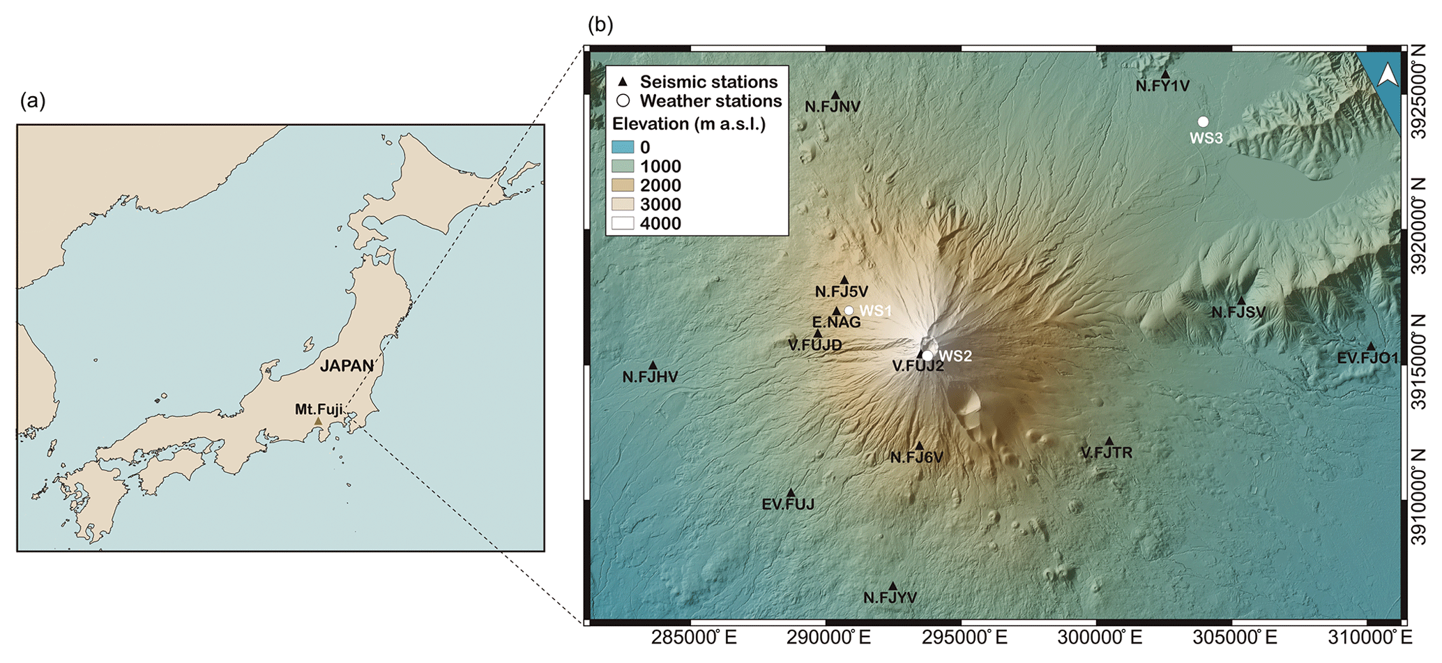
Figure 1 Overview map of Japan with the location of Mt. Fuji (a) and topographic map of the Mt. Fuji region (b) with the location of the 13 seismic stations and the 3 weather stations (WS1–WS3) used for this study. Seismic stations are labeled according to the institutions that operate them: N.F^* (NIED), EV.^* (ERI), V.^* (JMA), and E.NAG (NU and MFRI). Coordinates are given in UTM Zone 54N (JGD2000 datum) projection.

In this study, we applied the ASL method for the first time to locate snow avalanches and slush flows. Snow avalanches can adopt a variety of flow types from dry-snow avalanches, characterized by the typical powder cloud that usually hides a dense-flow region, to wet-snow avalanches that are characterized by a slower, plug-like flow. Slush flows are highly water-saturated avalanches that often entrain other types of debris. The ground motion generated is directly connected to the flow type of the avalanche (Pérez-Guillén et al., 2016). Our study area is the stratovolcano Mt. Fuji (Japan), where a dense, local seismic network is deployed for the study of the volcanic activity and the seismicity of the region (Fig. 1). Avalanches and slush flows, which appear to release almost yearly on all flanks of the volcano, are the dominant natural hazard at Mt. Fuji's present period since its last eruption in 1707. Large-size avalanches on the western and northern slopes have been reported since 1980 by the Yamanashi Road Corporation, whereas historical events have been determined by dendrochronology (Tanaka et al., 2008). Slush flows are often triggered by heavy rainfall events that destabilize the snowpack. Both types of flow attain run-out distances up to 4 km and destroy parts of the forest (Anma, 2007).

The next section characterizes the Mt. Fuji region and describes the instrumentation deployed around the volcano and the analysis of the avalanche or slush flow events by traditional methods. The ASL method for locating flows, the correction of the observed amplitudes by site amplification factors, and the seismic tracking of seven flow events are presented in Sect. 3. In Sect. 4, we use numerical simulations to reconstruct the avalanche trajectories and thus to assess the precision of the ASL method. We also estimate the average speeds of the flows from the seismic tracking and compare them with the numerically predicted speeds, and determine the limits of seismic detection with the local network (Sect. 5). We also examine possible correlations between source amplitude and seismic energy with the approximate run-out distance. Finally, a discussion of the main results and conclusions are presented in Sects. 6 and 7.

2 Observed avalanche and slush flow events at Mount Fuji

2.1 Study area

The stratovolcano Mt. Fuji is the highest mountain of Japan (3776 m a.s.l.) and located 100 km SW from the Tokyo metropolitan area (Fig. 1). The summit of the volcano towers almost 2000 m above all mountains within a range of 50 km. The mean annual temperature at the summit is −7 ^∘C, ranging from −20 ^∘C in February to +5 ^∘C in August (Anma et al., 1988). The annual precipitation at Mt. Fuji is about 2500 mm with frequent heavy-precipitation episodes that may exceed 200 mm in a few hours. As a typical stratovolcano, Mt. Fuji has gradual slopes that range from ∼10^∘ at low elevations (<1700 m a.s.l.) through ∼25^∘ at mid elevations to ∼35^∘ at high elevations (>2900 m a.s.l.). From winter to early spring, the slopes are usually covered by snow at elevations above 2000 m a.s.l. (Anma et al., 1988).

Figure 2 (a) Aerial photo of the snow avalanche #1 released on 13 March 2014 on the WNW flank (source: Asahi Shimbun Digital, https://www.asahi.com/, last access: 18 October 2019). The main flow impacted the road (path #1), and a secondary surge continued flowing downwards following path #2. (b) Photo of the deposits of avalanche #1 showing part of the forest damaged by the avalanche before the impact on the road (path #1). (c) Aerial photo of the large wet-snow avalanche #5 released on 14 February 2016 on the NE flank. The fracture of the slab was visually identified at a mean elevation of 3300 m a.s.l., and the flow split into two branches, #1 and #2. (d) Aerial photo of the wet-snow avalanche #6 released on 14 February 2016 on the WNW flank. The fracture of the slab was identified at a mean elevation of 3200 m a.s.l. The flow impacted the deflecting dam (#1), destroying some instruments. (e) Aerial picture of the deposits observed along the Osawa river at 1500 m a.s.l. from slush flow #7 that released on the W flank on 5 March 2018.

2.2 Instrumentation

A dense, permanent seismic network is installed around Mt. Fuji for monitoring its volcanic activity (Fig. 1). This local network consists of short-period (1 Hz) three-component seismometers with a sampling frequency of 100 Hz. These sensors are operated by the National Research Institute for Earth Science and Disaster Resilience (NIED); the Earthquake Research Institute, The University of Tokyo (ERI); and Japan Meteorological Agency (JMA). NIED stations are located at the bottom of boreholes at an approximate depth of 200 m from the surface, with the exception of station N.FY1V which is at a depth of ∼40 m; all other stations are positioned at the surface. In addition, a seismic station was temporarily installed by the Mount Fuji Research Institute (MFRI) and Nagoya University (NU) near an active avalanche path on the west flank at 2020 m a.s.l. (E.NAG in Fig. 1). This station was operative during the winters 2016 and 2017, recording data continuously with a sampling rate of 100 Hz. For this study, the raw seismic data from the different stations were first transformed to ground velocity (m s⁻¹) and all signals were filtered with a 4th-order Butterworth band-pass filter between 1 and 45 Hz (Pérez-Guillén et al., 2016).

Meteorological data were acquired by three automatic weather stations (WS1–WS3 of Fig. 1) located at different elevations of Mt. Fuji. WS1 and WS3 provide data of air temperature, precipitation, wind direction, and speed. WS2 at the summit of the volcano only measures air temperature. WS1 is operated by the Yamanashi Road Corporation and is set a few meters from E.NAG; WS2 and WS3 are operated by JMA.

2.3 Avalanche events

The small distance between the seismic sensors and the volcano flank (<10 km) allowed us to detect numerous avalanches and slush flows that released spontaneously in three high-precipitation episodes in 2014, 2016, and 2018 (Table 1). We used information about observed avalanche deposits, aerial photos, and weather data to constrain the time window within which to search manually for avalanche signals in the seismic data from the local network. Other seismic sources such as earthquakes could be discarded by comparing the candidate events with a regional seismic catalog provided by NIED.

Table 1 Information on the three avalanche episodes in 2014, 2016, and 2018: type (avalanche or slush flow) and number of the event, date, time of seismic detection, path, elevation of the release area, elevation of the deposition area, run-out distance, and flow duration recorded at V.FUJD. There is no visual data to verify the paths, release, or deposition areas of avalanches #2–#4 (not verified events).

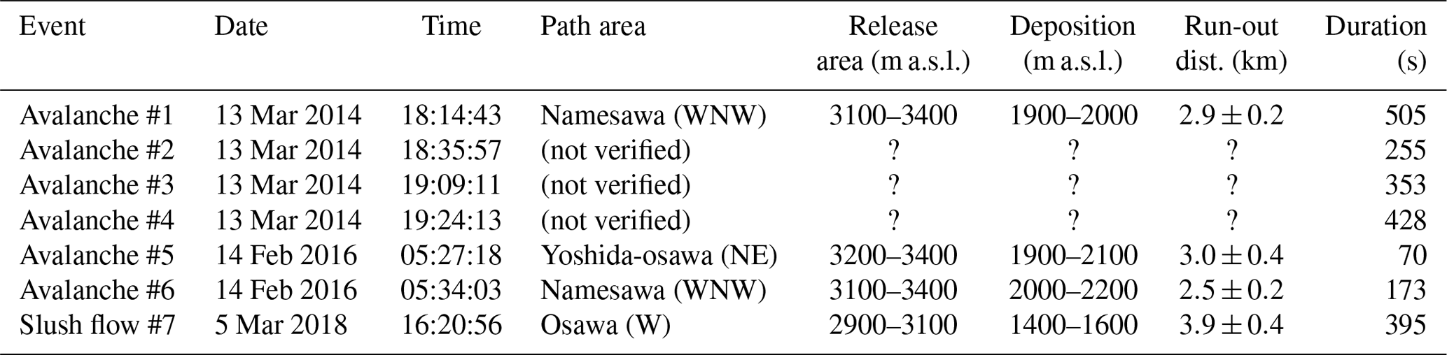
Figure 3 (a) Spectrogram (computed at V.FUJD station) and vertical seismograms generated by avalanche #1 released on 13 March 2014. Each trace is normalized by its maximum amplitude (peak ground velocity, PGV). (b) Spectrogram (V.FUJD station) and vertical seismograms generated by the consecutive avalanches #5 and #6 released on 14 February 2016. Each trace is normalized by the maximum amplitude generated by avalanche #5. Seismic data from N.FJ6V station were not available this day but there were data from the temporary E.NAG station. (c) Spectrogram (V.FUJD station) and time series recordings of the normalized vertical seismograms generated by slush flow #7.

2.3.1 The event of 13 March 2014

A spontaneous avalanche descended the Namesawa path, which is located at the west-northwest (WNW) flank of Mt. Fuji (avalanche #1 of Table 1), on 13 March 2014. An aerial photograph taken after the event shows the deposits of a large avalanche that impacted the road and destroyed part of the nearby forest (Fig. 2a and b). A run-out distance of 2.9±0.2 km (size 4–5 according to McClung and Schaerer, 2006) was estimated from aerial photos, the observed deposits, and damage. This avalanche was first seismically detected at 18:14:43 JST (Japan Standard Time) by the V.FUJ2 station (Fig. 3a), which is located at the summit of the volcano. At this time, the temperature recorded by WS2 at the summit of Mt. Fuji was −4 ^∘C. WS1 reported a temperature of +5 ^∘C and a cumulative precipitation of 140 mm in the 12 h before the avalanche; the wind speed ranged from 4 to 16 m s⁻¹ during the previous 24 h, blowing mainly from SE and S (Fig. 4).

Figure 4 Three-day time series of weather data measured by WS1 at 2020 m a.s.l. (Fig. 1) for the events of 2014 and 2016 (Table 1). The day #1 is 11 March 2014 for the 2014 events and 12 February 2016 for the 2016 events. (a) Time series of the mean air temperature (AT) and cumulative precipitation (CP). (b) Mean wind direction (WD) and wind speed (WS). Weather data from WS1 were not available on 5 March 2018.

The normalized vertical seismograms recorded at each location are shown in Fig. 3a, ordered according to increasing distance from the avalanche. V.FUJD was closest (∼1 km from the run-out area) and EV.FJO1 farthest at a distance of ∼20 km. In general, maximum amplitudes decrease as a function of distance to the source. However, some stations (V.^* and EV.^*) show great amplifications due to local site effects. This avalanche was detected by 11 seismic stations at a maximum distance of 15 km. The duration of the seismic signal is defined as the time interval in which the envelope of the signal exceeded a signal-to-noise ratio of 2, which is 505 s at the station V.FUJD (Table 1). The signals show the typical spindle shape of avalanche seismograms (Pérez-Guillén et al., 2016): a gradual increase in the amplitudes until the arrival of maximum amplitudes at 18:15:35 JST (Fig. 3a). The triangular increase in the spectrogram of V.FUJD (Fig. 3a) shows that the flow is approaching the sensor. The time interval of the maximum amplitudes is thus correlated with the arrival of the flow in the run-out area (path #1 of Fig. 2a), followed by a decrease in the amplitudes that is characteristic of avalanche deposition (from 18:15:45 to 18:16:10 JST). Another long wave packet, from 18:16:10 to 18:23:30 JST of Fig. 3a, is detected by the stations closest to the run-out area (V.FUJD and N.FJ5V). The spectrogram generated by this second surge is characterized by a temporal increase in the high-frequency energy content (up to 20 Hz; Fig. 3a), likely generated by a part of the avalanche that is slowly moving downwards, following a gully that approaches the location of V.FUJD (path #2 of Fig. 2a).

Three other candidate snow avalanches, #2–#4 of Table 1, were seismically detected in a time window of 2 h after the large avalanche. For these avalanches, no field observations or photos are available, hence the paths of these flows cannot be verified. The seismograms generated by these avalanches are shown in Fig. S1 in the Supplement.

2.3.2 The event of 14 February 2016

Two wet-snow avalanches descended almost simultaneously in the Yoshida-osawa path (northeastern flank; avalanche #5) and the Namesawa path (west-northwestern flank; avalanche #6) on 14 February 2016 (Table 1). Aerial photographs taken 2 d later show that the flow #5 split into two branches (#1 and #2 of Fig. 2c) and impacted the road on the NE flank. A large fracture line was identified at elevations of 3200–3400 m a.s.l., and the estimated maximum run-out distance was 3.0±0.4 km (size 5). This avalanche was seismically detected at 05:27:18 JST (Fig. 3.b). Avalanche #6 impacted the deflecting dam on the WNW path (#1 of Fig. 2d) and destroyed several instruments installed just beneath it so that the release time was known. A large seismic signal was first identified at 05:34:03 JST (Fig. 3b). The aerial photograph shows a fracture line at ∼3400 m a.s.l. (Fig. 2d). The observed deposits were a mixture of snow, ice, and rocks, the latter entrained at lower elevations where there was no snow. The estimated run-out distance is 2.5±0.2 km (size 4–5). An average temperature of +7.4 ^∘C and a cumulative precipitation of 134 mm were recorded by WS1 over the 12 h before the two releases (Fig. 4a). The wind speed ranged from 2 to 10 m s⁻¹ in the preceding 24 h, blowing from SSE and S (Fig. 4.b). The temperature recorded by WS2 at the summit of Mt. Fuji was −1.8 ^∘C.

The normalized vertical seismograms generated by these flows are shown in Fig. 3b. Avalanche #5 was detected by 11 seismic stations at a maximum source–receiver distance of 12 km, whereas avalanche #6 was detected by 8 stations at a maximum distance of 10 km. The seismograms of avalanche #5 show the usual spindle-shaped pattern of avalanche signals. However, the triangular shape of the spectrogram is not so well developed, with all the seismic energy concentrated below 10 Hz (Fig. 3b) due to the relatively large distance between V.FUJD and the moving flow (∼4–7 km). Despite the large dimension of avalanche #5, the duration of its signals (70 s at V.FUJD; Table 1) is shorter than for avalanche #6 (173 s at V.FUJD), mainly due to signal attenuation with distance. The longest signal duration for avalanche #5 (101 s) is recorded at N.FJ5V, the station that is closest to the flow path. The spectrogram of avalanche #6 shows an increase in the higher-frequency content up to 25 Hz when the flow approaches the dam in the run-out area (#1 of Fig. 2d) at ∼1.2 km from V.FUJD.

2.3.3 The event of 5 March 2018

A large slush flow in the Osawa valley on the western flank of Mt. Fuji was recorded by a camera installed at 1500 m a.s.l. (https://mobile.twitter.com/mlit_fujisabo/status/970587946934874112, last access: 18 October 2019) on 5 March 2018 at 16:23 JST (slush flow #7 of Table 1). The beginning of a large seismic signal was detected at 16:20:56 JST (V.FUJ2; Fig. 3c), lasting for 395 s. The deposits of the slush flow were detected along Osawa river at elevations of 1450–1600 m a.s.l. (Fig. 2e) during a survey on 11 March 2018. The estimated run-out distance was 3.9±0.4 km (size 5). Weather data from WS1 were not available on this day. The temperatures were −1 ^∘C at the summit (WS2) and +13.2 ^∘C at the foot of Mt. Fuji at 860 m a.s.l. (WS3). At this location, the cumulative precipitation during the 6 h preceding the slush flow was 26 mm.

The seismograms of slush flow #7 are characterized by several wave packets likely generated by different surges or internal parts of the flow (Fig. 3c). This flow was detected by eight seismic stations at a maximum source–receiver distance of 10 km (Fig. 3c). The high background noise recorded at V.FJTR, N.FJSV, and N.FJ1V is overlapping with the slush flow signal, hindering its identification. Maximum amplitudes and high-frequency content (up to 30 Hz) in the spectrogram, from 16:21:55 to 16:23:20 JST (Fig. 3c), correlate with the arrival of the flow in the run-out area and the video recording of the flow.

3 Avalanche location

3.1 Amplitude source location method

The ASL method exploits the progressive attenuation of seismic amplitudes with increasing distance. The method compares the recorded amplitudes at several sensor locations x_j with the expected amplitudes that are derived from fundamental properties of wave propagation, namely (i) attenuation due to geometrical spreading, (ii) attenuation due to absorption during propagation, and (iii) local site effects. The decay relationship of the seismic amplitude, u_j, at the jth station and instant t due to the attenuation of body waves with distance is expressed (Kumagai et al., 2010) as

$$\begin{array}{}\text{(1)}& u_j\left(t+{\displaystyle \frac{r_j\left(t\right)}{\mathit{\beta }}}\right)=A_{\mathrm{0}}\left(t\right){\displaystyle \frac{e^{-B{r}_j\left(t\right)}}{r_j\left(t\right)}},\end{array}$$

where $r_j\left(t\right)\equiv \left|x\right(t)-x_j|$ is the distance between the source and the jth station at time t, β is the seismic wave velocity, and A₀(t) the source amplitude. The factor 1∕r_j(t) accounts for purely geometric attenuation, while exp (−Br_j(t)) represents absorption with mean attenuation coefficient $B=\mathit{\pi }f/\left(Q\mathit{\beta }\right)$. B depends on the quality factor Q, the seismic velocity β in the medium, and the frequency f of the waves. The source amplitude is estimated from

$$\begin{array}{}\text{(2)}& A_{\mathrm{0}}\left(t\right)={\displaystyle \frac{\mathrm{1}}{N}}\sum _{j=\mathrm{1}}^N{u}_j^{\mathrm{o}}\left(t+{\displaystyle \frac{r_j\left(t\right)}{\mathit{\beta }}}\right)r_j\left(t\right)e^{B{r}_j\left(t\right)},\end{array}$$

where N is the total number of stations and $u_j^{\mathrm{o}}$ is the observed amplitude at station j. In order to use ASL to locate seismic events, the observed amplitudes should be corrected for local site effects that are caused by the variability in the terrain characteristics (e.g., different rock types, consolidated or unconsolidated sediments) at the locations of the seismic station. Therefore, we first estimated the site amplification factors using the coda method (Sect. 3.2) and then used these factors to correct the raw amplitudes at each station. Finally, the avalanche location x(t) is estimated by minimizing the residual

$$\begin{array}{}\text{(3)}& R\left(x\right(t\left)\right)={\displaystyle \frac{\sum _{j=\mathrm{1}}^N{\left[u_j^{\mathrm{o}}\left(t+r_j\left(t\right)/\mathit{\beta }\right)-u_j\left(t+r_j\left(t\right)/\mathit{\beta }\right)\right]}^{\mathrm{2}}}{\sum _{j=\mathrm{1}}^N{\left[u_j^{\mathrm{o}}\left(t+r_j\left(t\right)/\mathit{\beta }\right)\right]}^{\mathrm{2}}}}\end{array}$$

as a function of t. Equation (3) is minimized by sampling x at the nodes of a regular grid with a mesh spacing of 10 m. The source–sensor distances, r_j, were calculated using a digital elevation model (DEM) with 10 m resolution. The dimension of the grid was about 14 km (east) by 12.5 km (north), which includes all the potential avalanche paths of Mt. Fuji.

The ASL method uses the high-frequency seismograms generated by the recorded flows under the assumption of isotropic S-wave radiation. This assumption is valid in highly heterogeneous media, such as volcanoes, where multiple scattering of high-frequency S waves results in an isotropic radiation pattern (Kumagai et al., 2010; Morioka et al., 2017). Dominance of body waves over surface waves is highly plausible because surface waves are usually trapped in a shallow layer at the volcano surface (Yamamoto and Sato, 2010) and S waves are the dominant body waves in volcanic areas (Kumagai et al., 2010).

The observed vertical components were filtered using a band-pass filter between 4 and 8 Hz, which is the highest-frequency band with sufficient signal-to-noise ratio at the stations selected for source location. We estimated the mean amplitudes of the envelope using a 5 s wide sliding window, shifting it at 1 s increments. At each location, the amplitudes are corrected by the site amplification factors, and the emission-time window is shifted according to the S-wave travel times. We used a mean S-wave velocity of β=1400 m s⁻¹, typical of volcanic surface material (Ogiso and Yomogida, 2015; Kumagai et al., 2010). We tested the method for a range of S-wave velocities between 1300 and 2000 m s⁻¹. The results are not highly sensitive to the variation in the velocity. We obtained minimum residuals for a velocity of 1300 m s⁻¹. However, we localized the flows with a higher precision using a velocity of 1400 m s⁻¹. A quality factor Q=125 was adopted after testing a range of Q values. Ogiso and Yomogida (2015) used Q=100 to locate debris flows at Miharayama volcano on Izu Oshima island (Japan), which is located near Mt. Fuji, and they obtained the best flow locations for Q≥100.

3.2 Site amplification factors

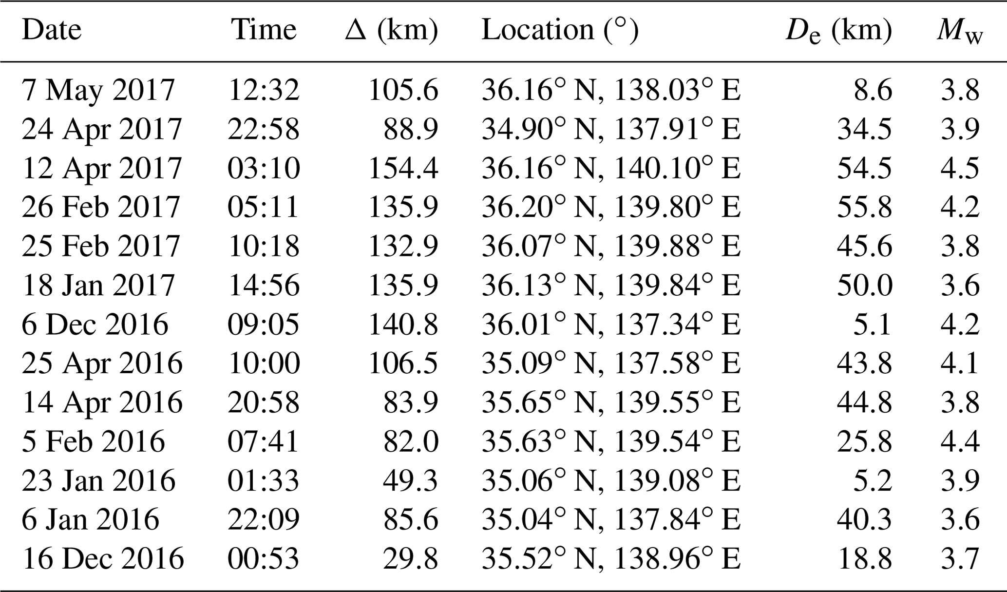
In the present study, the recorded seismic amplitudes at each station were corrected by site amplification factors that account for local site effects on seismic waves due to the topography and soil stratification. These factors are estimated by the coda method using earthquake records. Coda waves from local earthquakes are interpreted as backscattered waves generated by numerous heterogeneities in the crust. The ratio of coda-wave amplitudes from an earthquake is free of source and path effects and depends only on the local site amplifications for lapse times greater than twice the S-wave travel time (Aki and Chouet, 1975; Phillips and Aki, 1986). We selected 13 earthquakes with epicentral distances between 30 and 154 km (Table 2) from a seismic catalog provided by NIED. We determined the site factor of each station of the Mt. Fuji network relative to the reference station N.FJYV (Fig. 1) because the latter is located in a deep borehole and has low background noise.

Table 2 Date, time, epicentral distance (Δ), epicenter location (latitude, longitude), depth (D_e), and magnitude M_w of the local earthquakes whose coda waves were used to estimate the site amplification factors (source: JMA). Epicentral distances refer to the location of station E.NAG.

We calculated the envelopes of the vertical, band-pass-filtered signals in the four frequency bands 1–2, 2–4, 4–8, and 8–16 Hz. We selected five time windows of 10 s in length and 5 s of overlapping, starting at twice the travel time of the direct S wave. The amplitudes of the envelopes were averaged in each time window and the site amplification factors were estimated as the relative amplitudes between each station and the reference station (see Fig. 5a for the stations in boreholes and Fig. 5b for stations at the surface). Borehole stations are sheltered from surface ground noise and local site effects in the layers above them and therefore show low amplification factors that are mostly below 2. However, station N.FY1V, which is located in a more shallow borehole, shows higher amplifications with a maximum of 5.1 in the frequency band 2–4 Hz (Fig. 5a). Stations located at the surface show greater amplifications with values that range from 2 to a maximum of 7.5 in the highest-frequency band of V.FUJD (Fig. 5b).

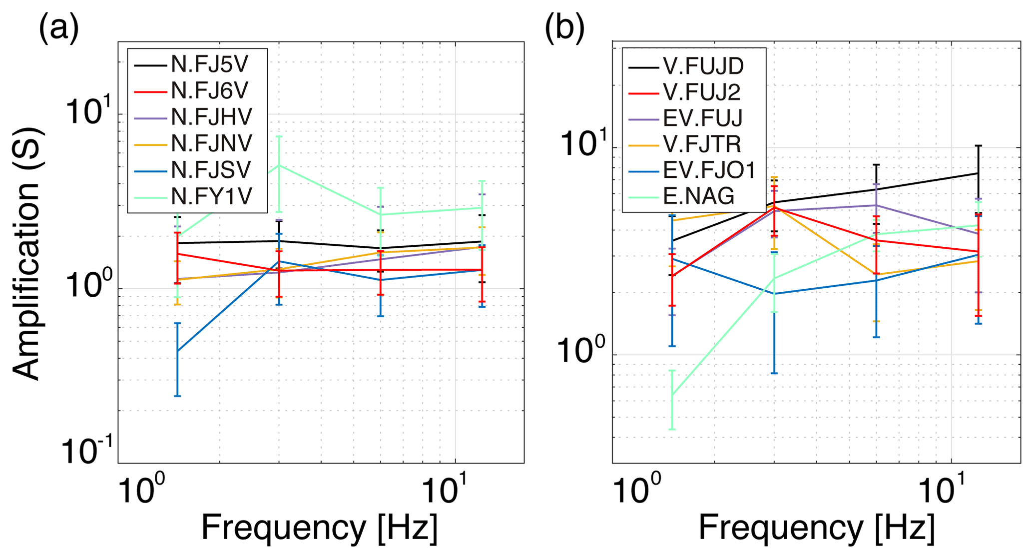
Figure 5 Site amplification factors (S) as a function of frequency estimated at the local network of Mt. Fuji, grouped by location: (a) borehole stations (NIED) and (b) surface stations (NU, ERI, and JMA).

Table 3 Event number, start (t₁) and end (t₂) times of source localization, spatial extent of the seismic locations (D_s), maximum source amplitude (A₀), and maximum radiated seismic energy (E_s).

3.3 Seismic tracking

For locating the recorded events, we use all stations that have a sufficient signal-to-noise ratio over a time interval from t₁ to t₂ (Table 3). We discard the initial and final parts of the signals generated by the flows because these are detected by too few sensors. The spatial distribution of the residuals is calculated for sliding time windows of 5 s length, shifted at 1 s increments. Figure 6 displays the residual distributions estimated for the observed events detected in two different time windows corresponding to the start time of the tracking (t₁) and a time interval of maximum seismic energy production by the flow. The location of the flow is estimated as the position of the minimum value of the residual distribution. The residual distributions show differences in the extent of the regions of small residuals and the location of their minimum values. Even though the regions of low residuals are quite large in the first time intervals of the tracking, the locations of the minima agree with field observations: avalanche #1 is estimated to be at 3180 m a.s.l. on the WNW side (Fig. 6a, upper panel), avalanche #5 at 2900 m a.s.l. on the NE side (Fig. 6b, upper panel), avalanche #6 at 3010 m a.s.l. on the WNW side (Fig. 6c, upper panel), and slush flow #7 at 2430 m a.s.l. on the W side (Fig. 6d, upper panel). The second set of residual distributions shows avalanche #1 at 2110 m a.s.l., which is 230 m from the NW road where it impacted (Fig. 6a, lower panel); avalanche #5 is estimated at 2270 m a.s.l., which is 140 m from the NE road where it impacted (Fig. 6b, lower panel); avalanche #6 is estimated to be at 2540 m a.s.l., which is in the middle of the flow path (Fig. 6c, lower panel); and finally slush flow #7 is estimated to be at 1500 m a.s.l., which is 90 m from the video camera that recorded the flow (Fig. 6d, lower panel).

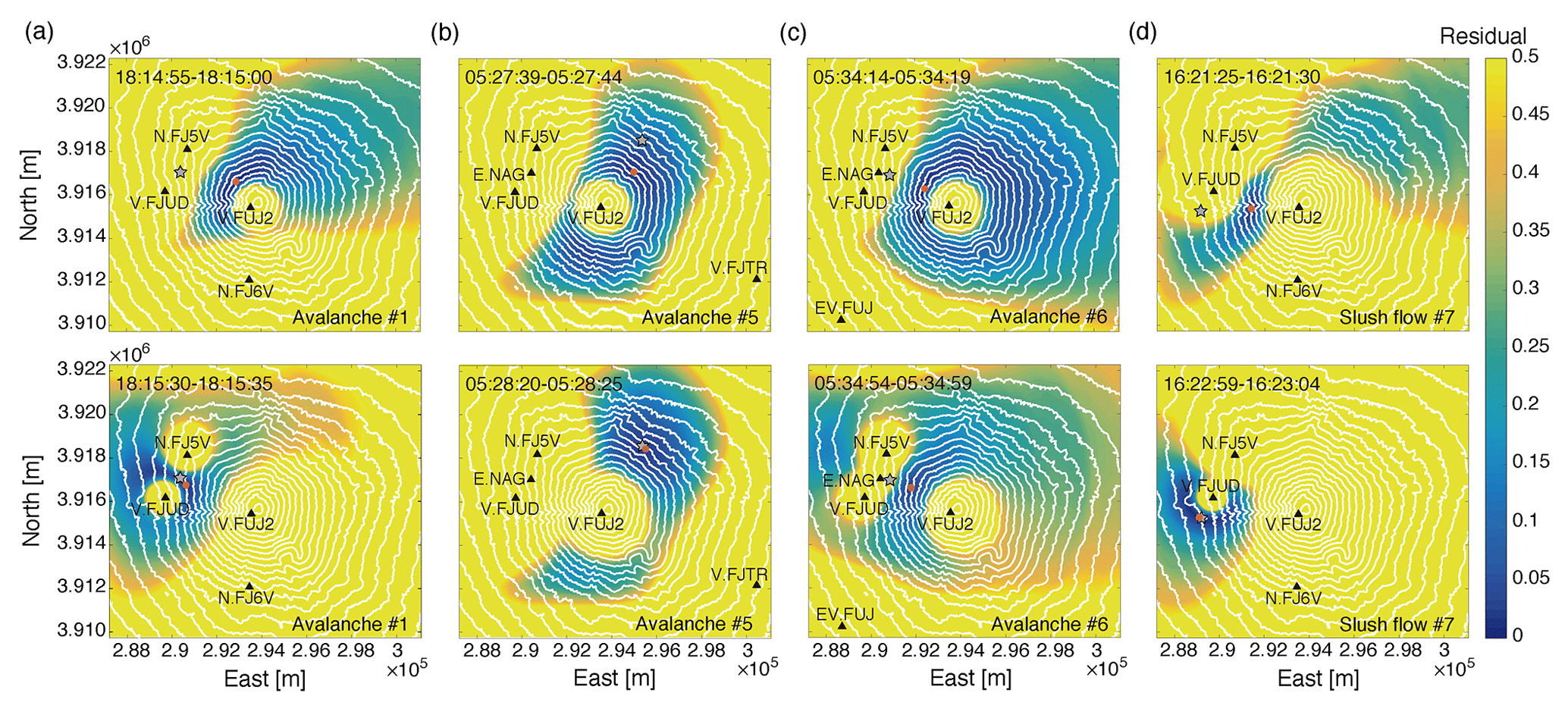
Figure 6 Maps of the spatial distributions of the residuals estimated for (a) avalanche #1, (b) avalanche #5, (c) avalanche #6, and (d) slush flow #7 at two different times: at the beginning of seismic tracking (t₁; upper panels) and at maximum source amplitude of the flows (lower panels). The asterisks mark specific locations of the run-out area of each flow: the road for avalanches #1 and #5, the dam for avalanche #6, and the video camera for slush flow #7. The red dots indicate the locations of minimum residual at the given instant.

A map of the locations of the minimum residuals estimated at each time interval for all the detected events (Table 1) is plotted in Fig. 7. The estimated locations of the visually identified flows are consistent with the field observations. For instance, the minimum residuals of avalanches #1 and #6 are confined to the Namesawa path on the WNW flank, avalanche #5 to the Yoshida-osawa path on the NE flank, and slush flow #7 to the Osawa valley on the W flank. In general, the locations move downwards in the flow direction. The estimated locations of the avalanches #2–#4 are on the W flank of Mt. Fuji (Fig. 7). Even though there is no direct observation to corroborate or reject this result, we scanned the historical Google Earth aerial pictures to verify if there are indeed three avalanches to be seen beyond avalanche #1. An aerial picture taken on 7 April 2014, approximately 3 weeks after event #1, shows deposits of avalanches that flowed through Osawa valley and a northern parallel path at the W flank of Mt. Fuji (Fig. S2). These paths correlate with the seismic locations estimated for the avalanches #2–#4.

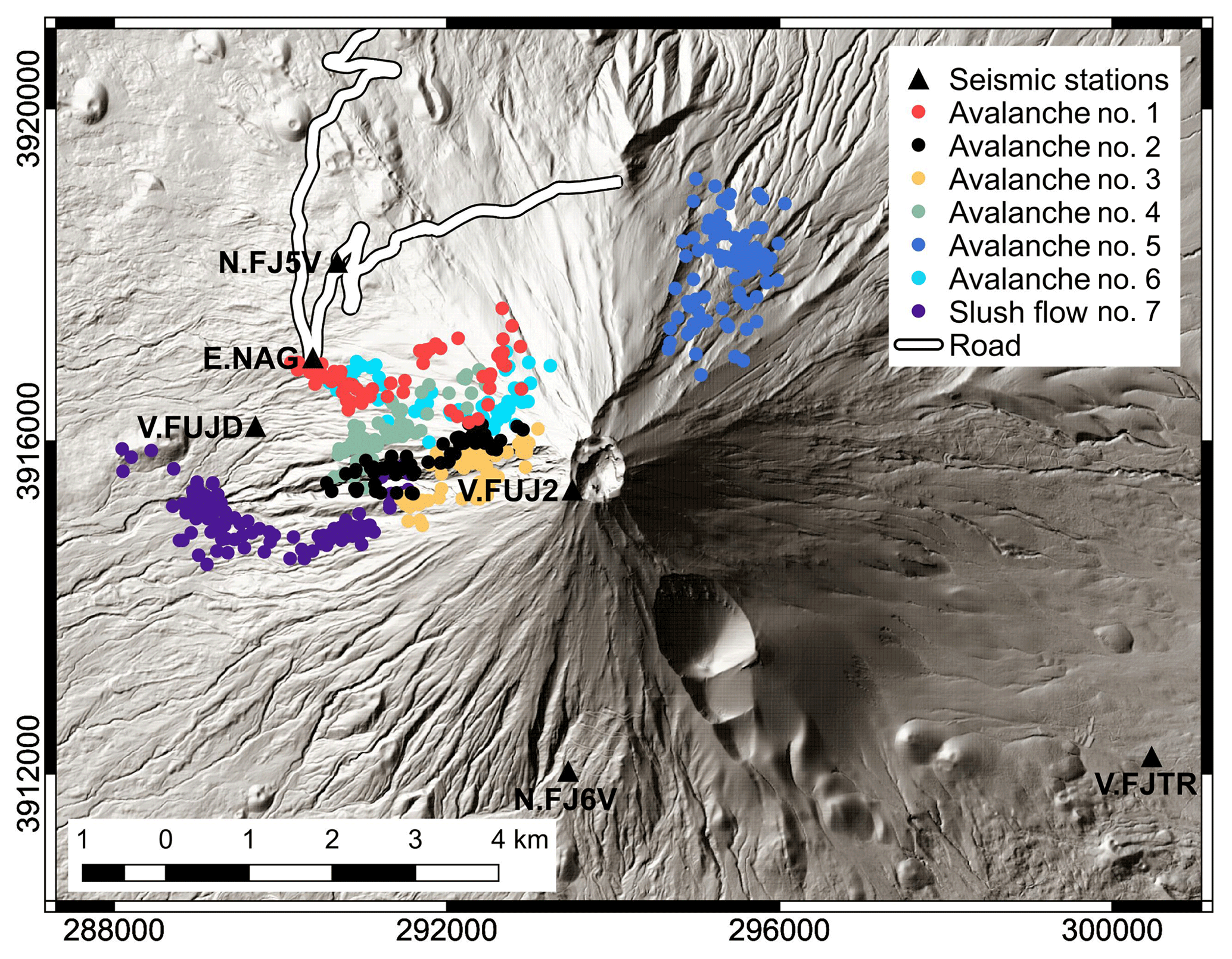
Figure 7 Map showing the seismic locations of the seven detected events as estimated by ASL (Table 1). Each flow is represented by a different color.

The seismic locations extend over a range of distances from 1.5 km (avalanche #4) up to 3.0 km (slush flow #7 of Table 3). Since only a part of the seismic signal is used to locate the flows, these distances (D_s of Table 3) are shorter than the maximum run-out distances estimated from field observations (Table 1).

3.4 Source intensity

The source amplitudes, A₀(t), computed according to Eq. (2), can be used as a quantitative measure of the size of the mass movement (Kumagai et al., 2013). We also estimated the seismic energy radiated by the mass flow, assuming a point source radiating over a hemispherical surface in an isotropic homogeneous medium in the frequency band of 4–8 Hz (Vilajosana et al., 2007b; Hibert et al., 2011):

$$\begin{array}{}\text{(4)}& E_{\mathrm{s}}\left(t\right)=\underset{t_{\mathrm{1}}}{\overset{t}{\int }}\mathrm{2}\mathit{\pi }\mathit{\rho }\mathit{\beta }{A}_{\mathrm{0}}^{\mathrm{2}}\left(t^{\prime }\right)\mathrm{d}{t}^{\prime },\end{array}$$

where E_s(t) is the radiated energy and ρ=2300 kg m⁻³ is the ground density (Kumagai et al., 2009). This energy represents a small fraction of the total radiated energy as it only considers a narrow frequency band of the vertical seismograms. Earlier studies showed that the main sources of the seismic waves generated by avalanches are (i) basal friction; (ii) the impacts of the flow on the snow cover, the terrain and the obstacles in the avalanche path; and (iii) erosion and dissipation processes (Biescas et al., 2003; Vilajosana et al., 2007b; Pérez-Guillén et al., 2016).

Figure 8 shows the source amplitude and seismic energy functions of all the avalanche events. Maximum values of these functions are shown in Table 3. Source functions are characterized by increasing amplitudes at the beginning of the motion, multiple local maxima, and decreasing seismic energy generation at the end of the motion. Accordingly, the seismic energy functions increase monotonously throughout the whole time interval, with larger rates during intervals of more intense generation of seismic energy (Fig. 8). The largest source amplitudes and seismic energies are generated by slush flow #7, which is the flow of largest size (size class 5). The source amplitude function of this flow displays three main local maxima at lapse times of 34, 61, and 95 s. At t=95 s, the location of the flow is estimated at 1500 m a.s.l., i.e., near the video camera (Fig. 6d, lower panel). Three different gullies converge there and the slope decreases to ∼10^∘. This topographic obstacle and the change in the slope are most likely responsible for this high seismic energy generation rate.

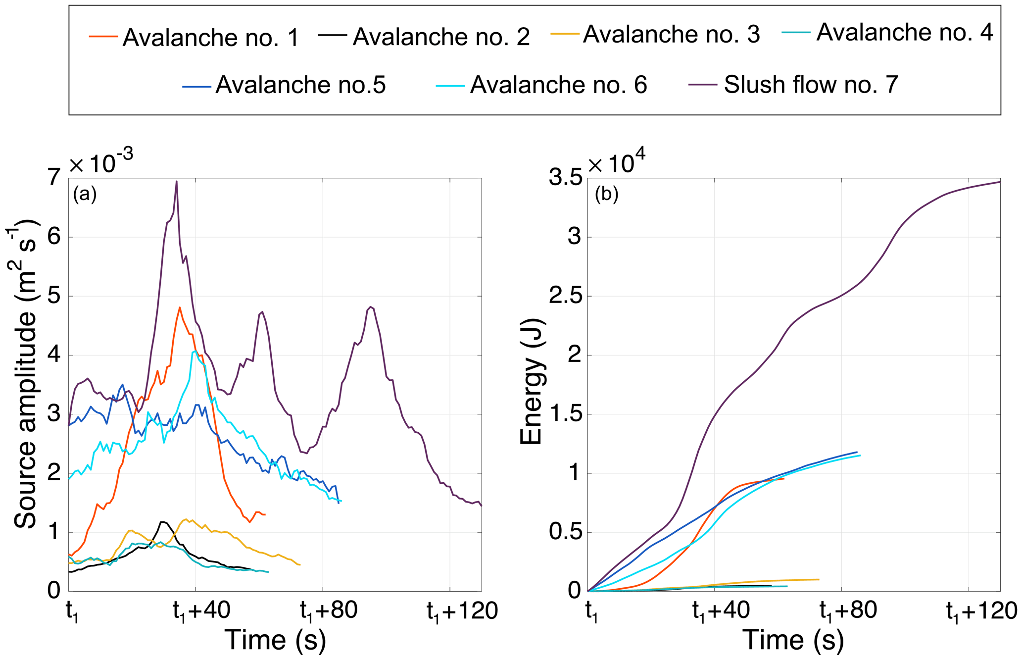
Figure 8 (a) Variation in the source amplitude estimated for the seven events as a function of time from the start time of the tracking window (t₁ of Table 3). (b) Temporal variation in the radiated seismic energies.

The second largest flow is avalanche #5, which shows a maximum seismic energy of 1.2×10⁴ J, which is slightly larger than the seismic energy generated by the consecutive flow #6 of smaller size (Table 3). For lapse times between 33 and 63 s, the source amplitudes of avalanche #6 are larger than the amplitudes of avalanche #5. This increase in the source amplitudes may be attributed to (i) lower attenuation of seismic energy radiated by flow #6 at lower elevations of its path due to the lack of snow cover on the west side of Mt. Fuji (Fig. 2d), (ii) higher basal friction due to the flow directly sliding on the ground, and (iii) entrainment of rocks and other debris observed in the deposits of this flow. Avalanche #1 is characterized by an emergent increase in the source amplitude up to the largest peak generated at t=35 s. At this time, the avalanche is close to the road (Fig. 6a, lower panel). For lapse times from 21 to 45 s, the source amplitude of this avalanche is larger than the source amplitudes generated by avalanches #5 and #6, showing that the impact of this flow with the forest and the road generated much seismic energy. The smaller avalanches #2–#4 show similar seismic energy generation rates, with maximum source amplitudes and energies up to 2 orders of magnitude smaller than the rest of the detected events (Table 3). The correlation between the flow size and the parameters presented here is investigated in Sect. 5.3.

4 Precision of source localization

4.1 Numerical flow simulations

We conducted numerical simulations of the avalanche flows with the numerical model Titan2D, an open-source code designed for simulating geophysical mass flows over complex topography (Patra et al., 2005). Titan2D solves the depth-averaged equations of mass and momentum for an incompressible continuum obeying a Mohr–Coulomb-type friction law in the shallow-water approximation. For Titan2D simulations, we have used a digital elevation model (DEM) of 5 m resolution provided by the Yamanashi Prefecture and Mt. Fuji's Sabo Office of the Ministry of Land, Infrastructure, Transport and Tourism (Japanese government). The model parameters are the internal friction angle of the flowing mass, ϕ, and the bed friction angle, δ, both of which may vary spatially. We used ϕ=40^∘ for all simulations since Takeuchi et al. (2018) confirmed that the internal friction coefficient does not significantly influence the results of simulations with Titan2D. The release volume is specified as h_ij(t₀)=h₀ if the grid point x_ij is inside a user-defined elliptically shaped domain on the surface, and 0 otherwise. The avalanche starts from rest, i.e., $u_{ij}\left(t_{\mathrm{0}}\right)=v_{ij}\left(t_{\mathrm{0}}\right)=\mathrm{0}$ for the slope-parallel velocity components u and v.

For adjusting the simulations of the visually identified flows, we determined the most likely bounds of the run-out distance from the aerial photos and the recorded damage (Fig. 2). A range of flow scenarios were simulated to find the best-fit model parameters and initial conditions for each avalanche or slush flow (Table 4). The flow depths simulated for events #1, #5, #6, and #7 are shown in Fig. 9. The release area of avalanche #1 is centered at 3250 m a.s.l. in the Namesawa path of the WNW flank (Fig. 9a). The simulation reproduces the deposition pattern satisfactorily if the bed friction angle is set to 20^∘ above 2500 m a.s.l. and to 25^∘ below 2500 m a.s.l. We increased the basal friction angle for the remainder of the avalanche path to account for the effect of the forest (Takeuchi et al., 2018) in addition to higher snow temperature. The maximum flow depth predicted for this avalanche is 5.25 m. The simulation recreates the impact of the flow on the road in the run-out area (Fig. 9a), where station E.NAG is located, in accordance with field observations (path #1 of Fig. 2a). Part of the simulated flow continues moving downhill through gully #2 (Fig. 2a) towards V.FUJD (Fig. 9a).

Figure 9 Flow depths simulated with Titan2D and estimated flow locations (blue points) from the seismic analysis of (a) avalanche #1, (b) avalanche #5, (c) avalanche #6, and (d) slush flow #7.

Table 4 Model parameters used for Titan2D simulations of events #1, #5, #6, and #7: event number, initial volume (V_i), fracture depth (h₀), elevation of the center of the release area (E), internal friction angle (ϕ), and bed friction angle (δ). Avalanches #1 and #6 are simulated with different values of δ above and below 2500 m a.s.l.

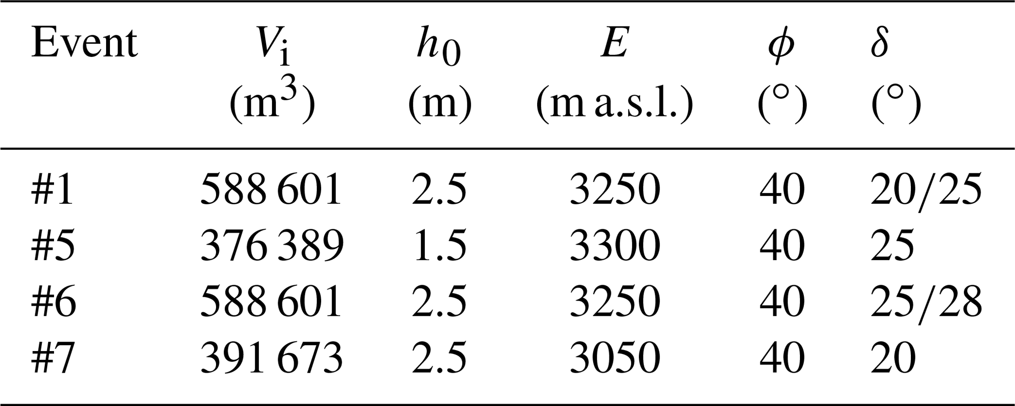
The release area of the simulation of avalanche #5 is centered at 3300 m a.s.l. in the Yoshida-osawa path of the NE flank (Fig. 9b). The bed friction angle is set to 25^∘ (Table 4). The simulation recreates the flow path adequately, showing that the flow splits into two branches and impacts the NE road in the run-out area at 2220 m a.s.l. (Fig. 9b), which is consistent with the observed deposits (Fig. 2c). The predicted maximum flow depth of this flow is 5.2 m. Avalanche #6 is simulated using the same release area and volume as avalanche #1 since both flows were triggered at the same site and followed similar paths. However, the run-out areas are different, with avalanche #6 impacting the deflection dam and depositing its mass above the road. With a variable bed friction angle ranging from 25^∘ above 2500 m a.s.l. to 28^∘ below 2500 m a.s.l., the simulation reconstructs the run-out area in agreement with these field observations (Fig. 9c). Owing to the lack of snow cover at mid-elevations on the western flank (Fig. 2d), we assigned a larger bed friction as the basal surface was directly the ground. The simulated maximum flow depth is 6.5 m. Slush flow #7 is simulated with an initial volume centered at 3050 m a.s.l. in the Osawa valley on the W flank (Fig. 9d). We used a bed friction coefficient of μ_b1=tan 20^∘ to fit the simulated slush flow with the observed run-out area (Fig. 2e). The simulated maximum flow depth is 7 m.

4.2 Precision of seismic localization

The numerical simulations were used as a reference for assessing the precision of the ASL method. We compared the seismic location at each time interval with the evolution of the simulated avalanche flow. Seismic locations could first be determined several seconds after the avalanche signal emerges from the noise at station V.FUJ2 at the summit of the volcano (Fig. 1), which is closest to the avalanche or slush flow release areas (Fig. 9). We also assumed an additional delay of a few seconds because the first movements of the avalanche are unlikely to generate enough seismic energy to be detected at a distance of >1 km. This second time delay was estimated by minimizing the mean error in the locations.

We defined the location precision as the minimum distance between the instantaneous area of the avalanche flow and the seismic location. We set this value to zero if the seismic location is within the avalanche flow. Figure 10 shows the location precisions and the residuals as a function of the lapse time from the start of the four simulations. The mean precisions are 154 m for avalanche #1, 115 m for avalanche #5, 85 m for avalanche #6, and 271 m for slush flow #7. Altogether, 25 % of the locations of avalanche #1, 37 % of the locations of avalanche #5, 34 % of the locations of avalanche #6, and 14 % of the locations of slush flow #7 are within the respective simulated flow areas (Fig. 9).

An interval of erroneous migrations of the seismic locations in northwestern direction is observed in the two flow events that descended the Namesawa path (Fig. 9a and c). The spurious migrations of avalanche #1 occur at 28–36 s (Fig. 9a) with location precisions over 400 m (Fig. 10a); avalanche #6 shows wrong migrations at 38–42 s (Fig. 9c) with location precisions over 300 m (Fig. 10c). Ogiso and Yomogida (2015) also observed migrations of the locations in a wrong direction, probably caused by an inadequate distribution of stations in that phase. The lack of stations close to the release area may explain the observed migrations in our case (Fig. 3a). The residual distributions in the first part of both signals also show that the region of small residuals extended in a NW direction (Fig. 6a and c, upper panel). Figure 9d also shows erroneous migration of the locations of slush flow #7 towards the southwest at 54–99 s, with location precisions over 400 m (Fig. 10d), and to the northwest at 100–104 s with location precisions over 900 m (Fig. 10d). The area of low residuals in the first part of the slush flow #7 signal extends in the SW direction (Fig. 6d, upper panel) and in the WNW direction at the end of the signal (Fig. 6d, lower panel). In general, the location precisions estimated for all the flows are under 500 m with peak values up to 900 m for avalanche #1, 640 m for avalanche #5, 630 m for avalanche #6, and 1260 m for slush flow #7.

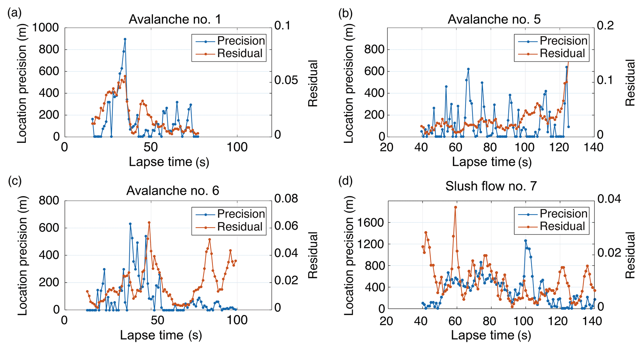
Figure 10 Location precisions and residuals estimated as a function of lapse time from the simulation start time of avalanche #1 (a), avalanche #5 (b), avalanche #6 (c), and slush flow #7 (d).

We also examined whether there is a correlation between the location precisions and the residuals. Avalanche #1 shows a moderate correlation with a Pearson correlation coefficient of r=0.64 and a p value of $p=\mathrm{1.9}\times {\mathrm{10}}^{-\mathrm{8}}$, which reflects strong certainty in the result. However, events #5–#7 show very weak correlations with coefficients below r=0.2.

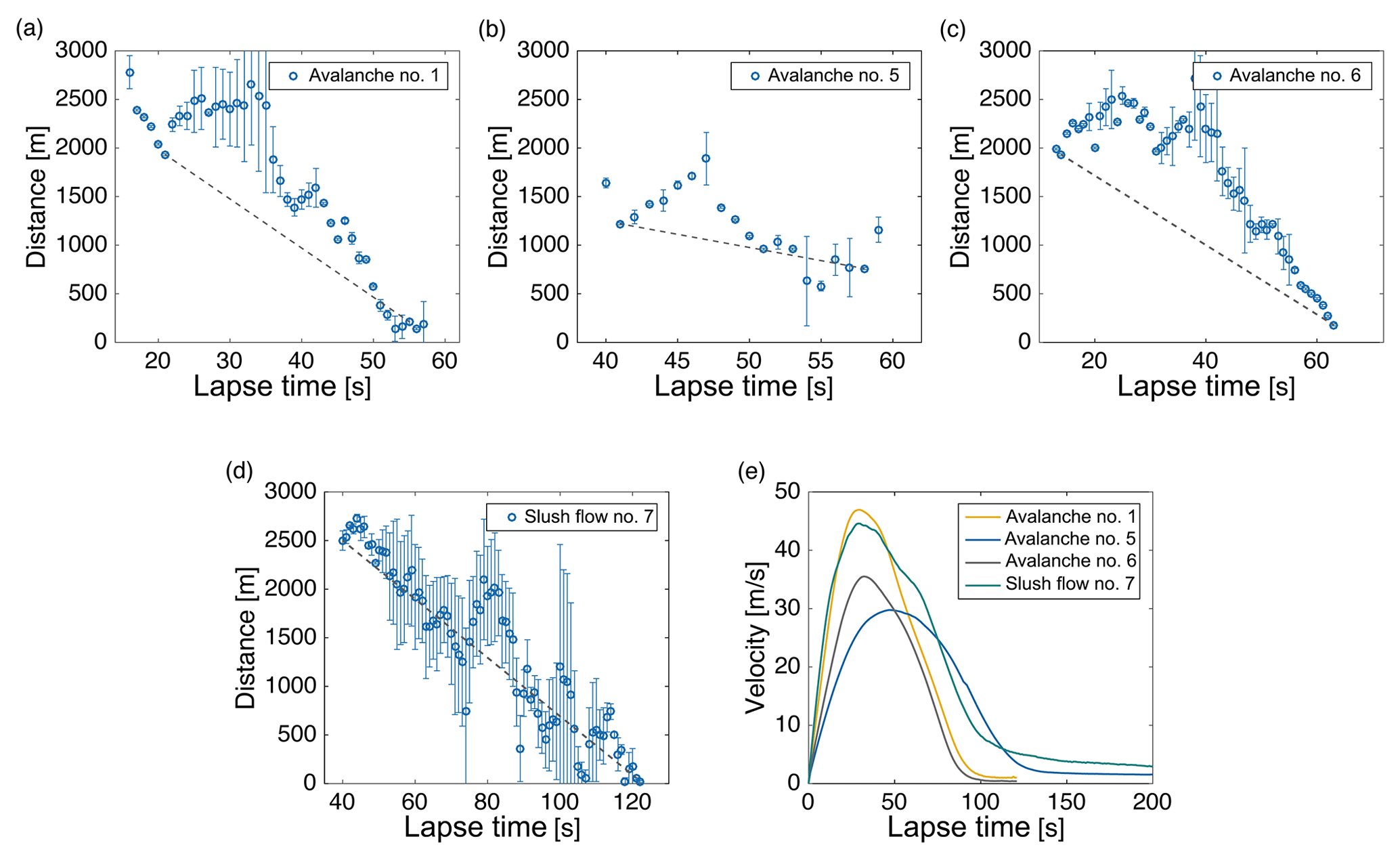
Figure 11 (a) Distance of ASL locations of avalanche #1 from seismometer E.NAG as a function of lapse time. (b) Distance of ASL locations of avalanche #5 from the NE road as a function of lapse time. (c) Distance of the ASL locations of avalanche #6 from the dam as a function of lapse time. (d) Distance of ASL locations of slush flow #7 from a run-out area location as a function of lapse time. The dashed gray lines connect the two points selected for estimating the mean speeds of each flow. (e) Simulated speed functions of avalanches #1, #5, #6, and slush flow #7.

5 Flow parameters

5.1 Average flow speed

The average speed of the flow can be deduced from the seismic tracking conducted in Sect. 3.3. We selected reference sites placed in the run-out area of each flow to compute the distance as a function of time between the seismic location and this site: E.NAG for avalanche #1, a location on the NE road for avalanche #5, the dam for avalanche #6, and for slush flow #7 a location on Osawa river close to the video camera that recorded the event. To estimate an average speed of each flow, we selected two seismic locations in the release area and the run-out area that are near the avalanche front and we computed the ratio of the distance traveled versus time. We discarded estimating the average speed from the linear regression of distance versus time because they also count times when the observed locations are far behind the front. We estimated the average speed of avalanche #1 at 51 m s⁻¹ (Fig. 11a), avalanche #5 at 27 m s⁻¹ (Fig. 11b), avalanche #6 at 36 m s⁻¹ (Fig. 11c), and slush flow #7 at 30 m s⁻¹ (Fig. 11d). Since avalanche #5 split into two well-separated branches before reaching the NE road (Fig. 9b), we estimated the mean speed in the time interval over which the flow is approaching the NE road. Figure 11e shows the speed functions of each flow simulated with Titan2D. The maximum flow speeds predicted by the numerical simulations are (Fig. 11e): 47 m s⁻¹ for avalanche #1, 30 m s⁻¹ for avalanche #5, 35 m s⁻¹ for avalanche #6, and 45 m s⁻¹ for slush flow #7. In addition, we compared the mean speeds estimated seismically with the ones predicted numerically. During the same time intervals, the mean speed estimated by Titan2D is 44 m s⁻¹ for avalanche #1, 29 m s⁻¹ for avalanche #5, 30 m s⁻¹ for avalanche #6, and 22 m s⁻¹ for slush flow #7. Hence, the average speeds estimated by the seismic locations of the avalanches #1, #5, and #6 are similar to the maximum values predicted by Titan2D, differing from the simulated average velocities by 0–6 m s⁻¹. The average speed estimated seismically of slush flow #7 exceeds the mean speed predicted by Titan2D by about 8 m s⁻¹.

5.2 Detection range

The detection range of the seismic network at Mt. Fuji is different for each recorded event. Figure 12 shows the source–receiver distances versus the run-out distances. For each event, the source–receiver distance varies during the flow motion and therefore we plot the maximum source–receiver distance for the seismic stations that detected the event and the minimum source–receiver distance for the seismic stations that did not detect the event. We estimated the detection range using the vertical component of the seismic signal and assuming for a detected event a minimum duration of the recorded signal of 10 s at each seismic location. The same assumption was adopted in previous studies of avalanches detected seismically (Lacroix et al., 2012; Hammer et al., 2017). The maximum detection distance is 15 km for avalanche #1. For the events #5–#7 the maximum detection radius is between 10 and 12 km, lower than the for avalanche #1 due to a higher background noise recorded on these days (Fig. 3). The detection radius of the three nonvisually identified avalanches released on 13 March 2014 is between 9 and 9.5 km from their seismically detected paths (avalanches #2–#4 of Fig. 7).

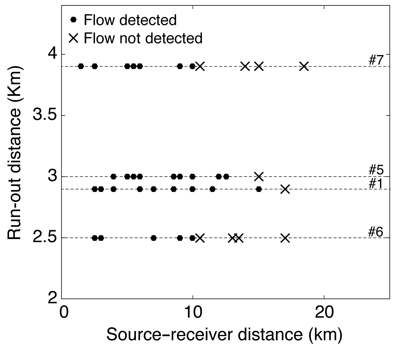
Figure 12 Run-out distances of the visually identified events versus the source–receiver distances estimated for each seismic location.

5.3 Flow size

We classified the size of each avalanche or slush flow event according to their maximum run-out distances. The events #5 and #7 are classified as extremely large events of size 5 according to the Canadian classification system for avalanche size (McClung and Schaerer, 2006), whereas avalanches #1 and #6 count as size 4–5. The nonvisually identified events, avalanches #2–#4, are classified as size 3–4 according to the length of their paths estimated by the ASL localizations. These extents of the seismic locations, here referred to as D_s (Table 3), are several hundreds of meters less than the run-out distances, i.e., between 75 % (avalanche #5) and 90 % (avalanche #6) of the maximum run-out distance. In order to correlate the size of each event and the seismic parameters of maximum source amplitude and energy, we used the known parameter D_s for all the events as a representative measure of the flow size. Figure 13 shows the fitting models between the maximum source amplitude (A₀ of Table 3) and energy (E_s of Table 3) versus the path length estimated seismically, D_s (m). The fits are (i) $A_{\mathrm{0}}=(\mathrm{4}\pm \mathrm{1})\times {\mathrm{10}}^{-\mathrm{6}}$ m s⁻¹ × $D_{\mathrm{s}}-(\mathrm{6}\pm \mathrm{2})\times {\mathrm{10}}^{-\mathrm{3}}$ m² s⁻¹ for the maximum source amplitude and (ii) $E_{\mathrm{s}}=(\mathrm{0.06}\pm \mathrm{1})\times {\mathrm{10}}^{-\mathrm{13}}$ J × $D_{\mathrm{s}}^{(\mathrm{4.8}\pm \mathrm{2.2})}$ for the energy. There is a high linear correlation (R²=0.95 in Fig. 13) between the source amplitude and the length of the avalanche path estimated by ASL, which is proportional to the maximum run-out distance. The best-fit model between the energy and the avalanche path is a power function (R²=0.92). We expect a power-law correlation to describe the physical size dependence of the radiated seismic energy better than an exponential function. The snow cover, which plays a decisive role in the generation and transmission of seismic energy (Pérez-Guillén et al., 2016), was different between events. The signals from the smallest events were probably also subjected to the strongest absorption in the snow cover, whereas slush flow #7 flowed largely over bare ground. Under comparable conditions, we expect the exponent of D_s to be less than in the obtained best fit.

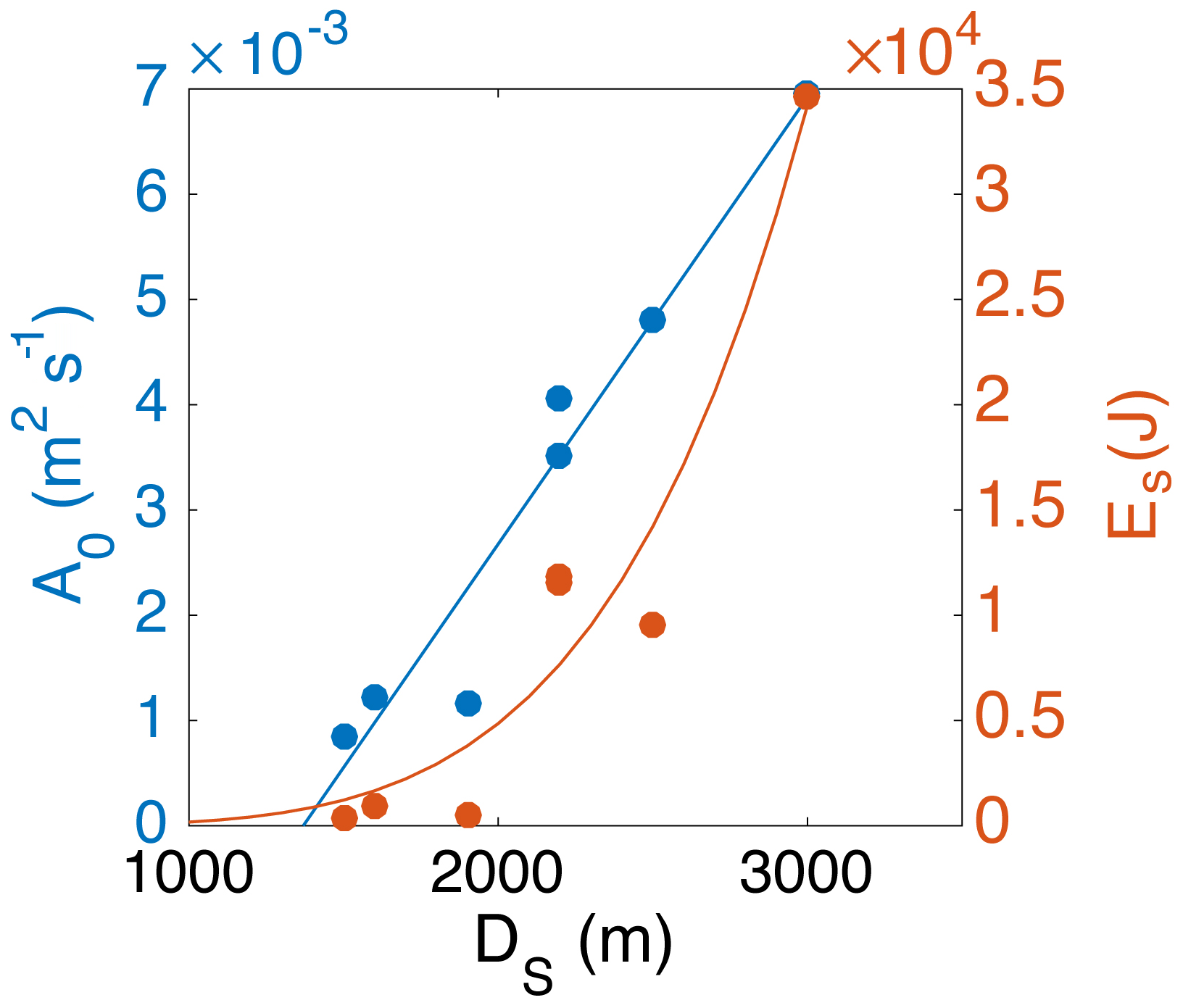
Figure 13 Maximum source amplitudes, A₀ (left in blue) and radiated energies, E_s (right in orange) versus spatial extensions of the seismic locations, D_s. The lines show the least-squares linear fitting of the source amplitude vs. distance (blue; R²=0.95) and the power-law fit of seismic energy vs. distance (orange; R²=0.92).

6 Discussion

6.1 Type of flows and correlation with weather patterns

We analyzed seven mass flow events that were spontaneously triggered at different flanks of Mt. Fuji during the winters of 2014, 2016, and 2018. These flows were detected using the local seismic network installed around the volcano. The signals were visually identified according to the typical features that snow avalanches display in the seismic recordings (e.g., Suriñach et al., 2001). The slush flow is characterized by similar signatures in the time and frequency domains, such as a long, spindle-like seismogram and a characteristic triangular shape of the spectrogram (Fig. 3c), which is mainly due to the variation in the source–receiver distance during the flow motion (Vilajosana et al., 2007a; Pérez-Guillén et al., 2016).

Knowing the release times of the flows accurately allowed us to identify the weather patterns that triggered them. In the first period of 13 March 2014, four snow avalanches were seismically identified in a time window of 2 h during a storm. The combination of heavy precipitation; strong winds, which accumulated drifted snow at higher elevations of Mt. Fuji; and an air temperature rise of several degrees (Fig. 4) was the main meteorological factor that led to the release of these avalanches. The temperature difference between the release area (<0 ^∘C) and the run-out area (>0 ^∘C) suggests that these avalanches started flowing as dry-snow avalanches and transformed into wet flows at lower elevations. Such flow-regime transitions are common in large avalanches due to variations in the snow cover properties, such as temperature and liquid water content, along the avalanche path (Köhler et al., 2018b, a). The heavy precipitation and warming episode of 14 February 2016 triggered two practically simultaneous wet-snow avalanches. They likely started moving as wet flows in the release area, where temperatures were around 0 ^∘C, and they may have transformed into slush flows – mixtures of snow and free water – due to the heavy rainfall in the lower part of their paths. The rapid melting of snow by heavy rain and warm temperatures on 5 March 2018 released a slush flow at high elevations of Mt. Fuji, which entrained water and sediments along its path. The video recorded at the deposition area (∼1500 m a.s.l.) shows a highly water-saturated debris flow (https://mobile.twitter.com/mlit_fujisabo/status/970587946934874112, last access: 18 October 2019).

Seismic waves are rapidly attenuated with distance, giving rise to a natural limit of detection of the signals generated by avalanches and slush flows. The range of detection of a seismic network varies depending on the type and size of flow, the characteristics of the terrain, and the background noise level. Hammer et al. (2017) used a seismic station of the Swiss seismological network to detect large wet-snow avalanches up to source–receiver distances of 8 times the avalanche run-out distances. At Mt. Fuji, the maximum distance of detection is 15 km for avalanche #1 with a run-out distance of 2.9 km (Fig. 12), yielding a source–receiver distance of about 5 times the avalanche run-out distance. The likely reason for the avalanche detection limit in this study being lower than in Switzerland is the strong scattering and attenuation beneath volcanoes (Kumagai et al., 2018), which are one of the most heterogeneous media of the Earth's crust (Yamamoto and Sato, 2010). The range of detection of wet flows is somewhat lower, with maximum source–receiver distances up to 4 times their run-out distances (events #5 and #6 of Fig. 12). The higher background noise caused by the severe weather conditions during the wet flow events is likely to be the principal reason for the reduced detection limit of these flows, considering that their source amplitudes are similar or even higher than for dry avalanches (Fig. 8 and Table 3). In addition, the higher water content in the interface between the flow and the terrain (particularly in slush flow #7) reduces the effective bed friction, which is one of the main sources of the seismic waves (Vilajosana et al., 2007b).

6.2 Mass flows localized by seismic methods

The localization of snow avalanches through their seismic signals is a challenging task because avalanche signals have no clear phase arrival, thus conventional methods for hypocenter determination are not applicable. Given the nature of these sources and the large intersensor distances of more than 1 km in Mt. Fuji's seismic network (Fig. 1), ASL is the most suitable method for locating the sources of the signals generated by these flows. ASL is based on the spatial distribution of the seismic amplitudes under the assumption of isotropic radiation of S waves (Kumagai et al., 2010). To obtain the spatial distribution of the amplitudes, it is imperative to correct for site amplification because this strongly affects the accuracy of the source locations (Kumagai et al., 2013). These amplification factors are frequency dependent and are much larger at stations located at the volcano surface due to unconsolidated deposits in the upper layers of the volcano. In the seismic network of Mt. Fuji, site amplification at the station V.FUJD is 6.3 times stronger than at the station N.FJYV (Fig. 5) in the frequency band of 4–8 Hz that is used for localizing the seismic sources. After correcting for the local amplification effects, we applied ASL for the first time to locate the snow avalanches and slush flows and demonstrated that the estimated locations (Fig. 7) are in good agreement with the observed flow paths (Fig. 2).

The precision of ASL is an important question in view of practical applications of the method to avalanches. Earlier applications of ASL to locate lahars (Kumagai et al., 2009) and debris flows (Ogiso and Yomogida, 2015; Walter et al., 2017) demonstrated that the flow paths were correctly identified by this method and the estimated locations were well constrained in the area of the observed deposits (Ogiso and Yomogida, 2015). Walter et al. (2017) measured the distance between the confined channel where a debris flow descended and the seismic locations estimated by ASL, giving an order of magnitude of the accuracy of the ASL locations between 100 to 900 m, but these accuracies were not estimated with regard to the temporal evolution of the flow. Kumagai et al. (2009) performed numerical tests using synthetic waveforms generated by a vertical single source at a given location of the volcano and then applied ASL to determine its location, finding that both locations differed slightly. They also tested the method with two simultaneous and spatially well-separated sources at the volcano. The minimum residual was located between the two sources, with a broad area of small residuals between them. This result may explain why some of the ASL locations of avalanche #5 are between its two branches for lapse times of t>60 (Fig. 9b) and why the region of small residuals then is fairly large (Fig. 6b, lower panel). How to analyze situations with multiple simultaneous sources with ASL is an important issue to address because avalanches and slush flows are extended sources of seismic energy on the scale of the source–receiver distance.

Ideally, the precision of ASL should be studied at an avalanche test site, where video recordings and radar measurements provide comprehensive information about the location and extent of the avalanche through time. At Mt. Fuji, only limited information about the location of the fracture line and the run-out area is available for four events (Fig. 2). Numerical flow simulations can fill this gap to some degree: the initial conditions as well as one to several model parameters can be varied independently until the deposit location and any other available constraints are satisfactorily reproduced. The time evolution of the best-fit Titan2D simulation can then be compared to the time series of seismic localizations. Using this approach, the mean location precisions are between 85 m (avalanche #6) and 271 m (slush flow #7) with point-wise maximum location precisions up to ∼1 km (Fig. 10). This precision is similar to that of previous applications of ASL (Walter et al., 2017).

The only two previous studies of avalanches localized by seismic methods were based on array techniques (Lacroix et al., 2012; Heck et al., 2018b), which are not applicable with Mt. Fuji's network due to the configuration of the seismic stations. Array techniques allow for computing the back-azimuth of the incoming wave field, which is then compared to known avalanche paths. Lacroix et al. (2012) tracked the location of 80 snow avalanches in the French Alps, estimating the precision of azimuth determination to about 15^∘ based on a correlation criterion. The corresponding location errors amount to several hundred meters – similar to the ASL location precisions estimated in this study (Fig. 10).

6.3 Inferring flow properties from seismic data

Kumagai et al. (2013) found a scaling relationship between the magnitude and the source amplitudes of different seismic signals from volcanoes (explosions, volcano-tectonic earthquakes, and long-period events), showing the feasibility of using them to quantify their size. In addition, Kumagai et al. (2015) showed that the source amplitudes of lahars increase linearly with the cumulative source amplitudes, but a scaling relationship between them and the size of the lahar was not deduced. They estimated the source amplitudes of the lahars on the order of $\sim {\mathrm{10}}^{-\mathrm{2}}$ m² s⁻¹, which is 1 order of magnitude larger than the source amplitudes estimated in this study (Fig. 13). Ogiso and Yomogida (2015) also estimated the source amplitudes generated by five large-size debris flows using ASL. The maximum source amplitudes of these flows in the frequency band of 5–10 Hz were in the range of $(\mathrm{1}-\mathrm{4})\times {\mathrm{10}}^{-\mathrm{3}}$ m² s⁻¹. Even though our amplitudes are estimated in a slightly different frequency band of 4–8 Hz, these values are on the same order of magnitude as the source amplitudes estimated for our events (Fig. 8), suggesting that the size of those debris flows is similar to the size of the avalanches and slush flow released at Mt. Fuji.

The two parameters deduced by the ASL method, D_s and A₀ (Table 3), can be used as quantitative measures of the event size as D_s is proportional to the maximum run-out distance and A₀ is linearly correlated with D_s (Fig. 13). In addition, another size-scaling relationship between D_s and the radiated energy was found. Previous studies found different scaling relationships between the radiated seismic energy and, for example, the duration of rockfalls (Hibert et al., 2011; Levy et al., 2015) or the kinetic energy of debris flows (Coviello et al., 2019). We estimated the radiated seismic energy of the flow following the simplified approach used by Vilajosana et al. (2007b) and Hibert et al. (2011). At volcanic areas, however, the diffusion model is more appropriate for modeling seismic energy transport as it reflects multiple scattering of the seismic energy due to the heterogeneities of the volcano (Yamamoto and Sato, 2010). The maximum energy values estimated are on the order of 10⁴ J (Table 3). These values are low compared to the estimated seismic energies (∼10⁶ J) of two avalanches of size 4 in Norway (Vilajosana et al., 2007b) or other types of mass movements such as lahars (Walsh et al., 2016), debris flows (Coviello et al., 2019), and rockfalls (Hibert et al., 2011; Vilajosana et al., 2008; Levy et al., 2015; Guinau et al., 2019), which range between 10³ and 10⁹ J depending on the type of flow and its size. In this study, we consider only a narrow frequency band of the spectra so that our values represent only a small fraction of the total generated seismic energy. Moreover, none of the previous studies corrected the seismic amplification for site effects before estimating the seismic energy.

Using ASL localizations at different times, we can estimate the average front speed of a flow (Sect. 5.1). We obtained a maximum speed of 51 m s⁻¹ for the dry-snow avalanche #1. The typical speeds measured in large dry-snow avalanches of size 4–5 range widely from 40 up to 70 m s⁻¹ (Gauer et al., 2007a, b; Köhler et al., 2016). The estimated speeds of wet flows detected in this study (Fig. 11) are on the order of 30 m s⁻¹, similar to the front speeds measured for large wet-snow avalanches (Gauer et al., 2007a).

7 Conclusions

Large avalanches and slush flows are often released at different flanks of Mt. Fuji and can be detected by the local seismic network at distances up to 10–15 km. Using the analysis from several sensors of this local network, we successfully applied the ASL method to localize the seismic signals generated by the avalanches and slush flows at Mt. Fuji. The ASL method has proven to be a useful technique for locating the position of these flows in an extended area where a seismic network with a large intersensor distance of more than 1 km is available. Our results show that it is feasible to determine in which path an avalanche descended, to track the avalanche flow with reasonable precision (on the order of magnitude of 100 m), and to infer additional flow properties such as the approximate run-out distance and the average speed of the flow. This is the first time dynamical properties characterizing avalanches and slush flows at Mt. Fuji have been measured. These parameters are necessary for calibrating dynamical models for applications at Mt. Fuji, such as for the design of structural protection measures against these hazardous mass movements. In addition, the size-scaling relationships obtained here will be useful when establishing an empirical seismic method for quantifying the size of the detected mass flows, independently of the type of flow (avalanches and slush flows), path location and orientation. All this information is of great value for assessing avalanche hazard on Mt. Fuji, given that in most cases seismic records are the only available information on snow avalanche and slush flow events.

An important task in the near future will be to develop highly effective methods for automatically detecting and tracking avalanche events in the seismic data in near-real-time. A first challenge to achieve this aim will be developing reliable algorithms to discriminate between avalanches and other seismic sources (e.g., Heck et al., 2018a, 2019) or in training a system based on machine learning. Once the avalanche has been successfully identified in the seismic records, ASL can be easily automated in several data processing steps, providing the path location and tracking of the mass flow event. Such a tool can be applied in avalanche-prone areas of many regions and will be an economical tool supporting the authorities in the management of avalanche risk. Specifically, many volcanic areas are equipped with dense seismic networks and could benefit from this inexpensive method for locating mass movements and inferring their dynamical properties.