the Creative Commons Attribution 4.0 License.
the Creative Commons Attribution 4.0 License.
Drainage divide networks – Part 2: Response to perturbations
Wolfgang Schwanghart
Drainage divides are organized into tree-like networks that may record information about drainage divide mobility. However, views diverge about how to best assess divide mobility. Here, we apply a new approach of automatically extracting and ordering drainage divide networks from digital elevation models to results from landscape evolution model experiments. We compared landscapes perturbed by strike-slip faulting and spatiotemporal variations in erodibility to a reference model to assess which topographic metrics (hillslope relief, flow distance, and χ) are diagnostic of divide mobility. Results show that divide segments that are a minimum distance of ∼5 km from river confluences strive to attain constant values of hillslope relief and flow distance to the nearest stream. Disruptions of such patterns can be related to mobile divides that are lower than stable divides, closer to streams, and often asymmetric in shape. In general, we observe that drainage divides high up in the network, i.e., at great distances from river confluences, are more susceptible to disruptions than divides closer to these confluences and are thus more likely to record disturbance for a longer time period. We found that across-divide differences in hillslope relief proved more useful for assessing divide migration than other tested metrics. However, even stable drainage divide networks exhibit across-divide differences in any of the studied topographic metrics. Finally, we propose a new metric to quantify the connectivity of divide junctions.
- Article
(8229 KB) - Full-text XML
- Companion paper
- BibTeX
- EndNote
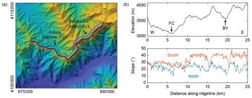
Figure 1Example of a mobile drainage divide in the Hindu Kush, Afghanistan. (a) Digital elevation model draped over a hillshade image. Colors denote elevations that range from ∼2000 m (blue) to ∼4000 m (yellow). The black line traces the drainage divide with clear signs of mobility. The center of the map lies at approximately 37.10∘ N and 71.06∘ E. North is up and the UTM zone is 43. (b) Profiles of the elevation (upper panel) and mean slope (lower panel) along the drainage divide shown in panel (a). Mean slope angles were computed along swath profiles that extend 500 m to the north (blue) and south (red) of the drainage divide.
Divide migration is a time-dependent process that is difficult to quantify. While the effects of regional-scale drainage captures may be preserved within sedimentary archives (e.g., Clift et al., 2006), this is unlikely for smaller-scale drainage captures or gradual divide migration. In such cases, most studies rely on topographic indicators. Mobile divides are typically inferred from post-drainage-capture evidence: distorted drainage structures, low divides (wind gaps), or high tributary junction angles (e.g., Clark et al., 2004) (Fig. 1). However, divide mobility may also be expressed in the topography without major drainage captures or flow reversals but as a result of the more gradual migration of divides. Willett et al. (2014) inferred drainage divide mobility from across-divide differences in χ values, a proxy for steady-state river channel elevation (Perron and Royden, 2013). They argued that changes in drainage area within mountain ranges, e.g., due to tectonic strain of the crust (Yang et al., 2015), may commonly lead to relative differences in incision rate and the formation of low-relief landscapes that are bordered by migrating divides. Whipple et al. (2017a, b), however, argued that the timescale of such changes is too short to profoundly affect mountainous landscapes. Instead, they argued that transient low-relief landscapes, such as those in southeastern Tibet, are more likely to be formed by regional changes in rock uplift rate and upstream propagation of knickpoints between the adjusted and unadjusted parts of landscapes. They also cast doubt on the ease of comparing across-divide differences in drainage network geometry (i.e., χ values) where the common base level is far and opposing rivers may incise into areas of different rock types, different rock uplift rates, or different climates. Whipple et al. (2017a, b) instead proposed that the shape of drainage divides themselves holds clues about their mobility (Fig. 1). Amongst the topographic parameters that they tested are across-divide differences in channel elevation at a reference drainage area, mean headwater hillslope gradient, and mean headwater local relief.
In summary, several different metrics have been proposed that may allow for the quantification of divide mobility in both natural and modeled landscapes. Forte and Whipple (2018) compared the performance of these metrics with a landscape evolution model in which they induced divide mobility and concluded that across-divide differences in relief or gradient better depict divide motion than χ. In their analysis, however, they focused on divide motion that is perpendicular to the regional drainage direction and averaged divide migration rates as well as topographic metrics across the entire width of the model domain so that each time step is associated with single values for divide migration rate, erosion rate difference, and the tested topographic metrics. In part 1 of this study (Scherler and Schwanghart, 2020a), we presented a new approach for the automatic identification and ordering of drainage divide networks in a digital elevation model (DEM), which removes the necessity of manually selecting drainage divides for comparison. Here, we present experiments with a numerical landscape evolution model that we conducted to investigate how drainage divide networks respond to different perturbations, including fault activity and differences in erodibility. In contrast to previous studies that examined the response of drainage divides to perturbations, we studied the entire drainage divide network in an objective manner and examined how different portions of the divide network respond to perturbations. In addition, we tested the utility of a new metric that quantifies the connectivity of drainage divide junctions.

Figure 2Graphical representation of the model setups in the landscape evolution experiments. The starting condition of each model is shown at the top of each rock column. During the experiments, the entire rock column is eroded and deeper-lying regions are exhumed. (a) “Initialize” started from a nearly flat surface and reached steady-state topography; the end of Initialize provided the starting point for all other models. (b) “Reference” included no changes. (c) “Rotating” included a circular left-lateral strike-slip fault active throughout the experiment. (d) “Inclined” included 1 km thick and 5 km spaced layers of 50 % reduced erodibility, dipping 30∘ towards northwest. (e) “Spheres” included 30 randomly assembled spheres of 3 km diameter with 75 % reduced erodibility.
2.1 Landscape evolution model
We studied the response of divide networks to stream captures and divide migration using the TopoToolbox Landscape Evolution Model (TTLEM; Campforts et al., 2017). In our experiments, we modeled the topographic evolution of a 20 km × 20 km square block (50 m node spacing) subject to uniform rock uplift, stream-power-based fluvial incision (e.g., Howard and Kerby, 1983; Whipple and Tucker, 1999), and hillslope diffusion (e.g., Culling, 1963):
where z is elevation (L), t is time (T), U is rock uplift rate (L T−1), A is upstream area (L2), S is local channel slope (L L−1), Kr is a parameter of the efficiency of river incision (T−1) ( yr−1), and m and n are dimensionless constants with values of 0.5 and 1, respectively. The last term on the right-hand side depicts elevation change due to the divergence in diffusive hillslope transport qs (L3 L−1 T−1), which we consider to be a linear function of hillslope gradient: , where D is the diffusivity (L2 T−1) of soil creep ( m2 yr−1). All four edges of the block were fixed in elevation (z=0 m), which forced rivers to flow outwards. The uplift rate (U=1 mm yr−1) was constant in all models. Our choice of parameter values was guided by the study of Whipple et al. (2017b), who tested a wide range of rock uplift and erosional efficiency parameters and found almost no difference of divide mobility in models with and without hillslope diffusion and for n values of 1 and 2.
We started from a flat surface with imposed random noise and ran the experiment for 30 Myr until the topography reached a steady state. The result of this model, which we termed “Initialize”, provided the starting point for four other models that we ran for 10 Myr (Fig. 2). The model “Reference” included no further changes. In the model “Rotating”, we included a circular (10 km diameter) left-lateral strike-slip fault that was active throughout the experiment. Strike-slip faults are well known for enforcing drainage captures and thus divide mobility (e.g., Castelltort et al., 2012; Duval and Tucker, 2015). Although the rotating block has, to our knowledge, no real-world equivalent, this model setup represents a convenient way of simulating extended periods of strike-slip faulting, as the fault does not intersect the model boundary (Braun and Sambridge, 1997). The fault slip rate was fixed at 4 mm yr−1, which corresponds to an angular velocity of rad yr−1, resulting in ∼460∘ of total rotation during the model run. We note that the rotating movement requires interpolation and thus leads to numerical diffusion of elevations within the rotating disk. However, the resulting change in total volume by interpolation is <0.03 % of the volume uplifted during the same time and therefore small. The model “Inclined” included 1 km thick and 5 km spaced layers of 50 % reduced erosional efficiency of rivers (Kr), dipping 30∘ towards northwest. The Inclined model is representative of a landscape in which rivers incise into tilted sedimentary rocks of nonuniform rock strength, similar to what has been studied by Forte and Whipple (2018). During the experiment, the combination of surface lowering and inclination resulted in the resistant layers regularly sweeping from southeast to northwest across the simulated landscape. The model “Spheres” included 30 randomly assembled spheres of 3 km diameter with 75 % reduced erosional efficiency of rivers (Kr). This experiment may represent incision of a region that is characterized by country rocks with more resistant magmatic intrusions. The expected behavior of this model is similar to the landscape response to localized perturbations studied by O'Hara et al. (2018).
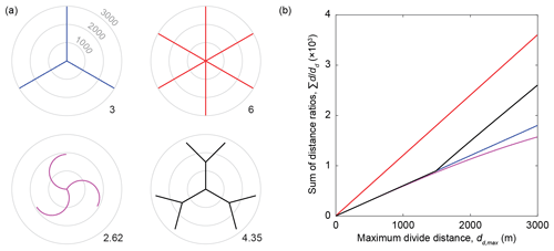
Figure 3Illustration of the junction connectivity (CJ) of different drainage divide junctions. (a) Map view of four hypothetical divide junctions. Gray circles indicate Euclidean distance from the junction. Numbers to the southeast in each map give the CJ value based on a dd,max of 3000 m. (b) Sum of distance ratios (; cf. Eq. 3) as a function of the maximum divide distance for each case in panel (a).
2.2 Topographic analysis
We analyzed the modeled topography and the associated drainage divide network. For each modeled topography and at each time step (dt=40 000 years), we first computed flow directions and flow accumulation, and we subsequently identified the stream network using a drainage area threshold of 0.2 km2. We next derived the drainage divide network on the basis of the stream network and using the algorithm proposed in Scherler and Schwanghart (2020a). We calculated divide distances and divide orders based on the Topo ordering scheme (Scherler and Schwanghart, 2020a). As topographic metrics, we included elevation (z), hillslope relief (HR), and horizontal flow distance to the stream network (FD). HR was measured as the elevation difference between a point on the divide and the nearest river location as measured by the distance along local flow directions. We also computed χ values on either side of a divide using a reference area A0 of 1 m2, a reference concavity θref of 0.45, and setting the base level xb to 0 at the edge of the model domain (e.g., Perron and Royden, 2013):
For each divide edge, we computed these topographic metrics and the erosion rate (Eq. 1) for the two neighboring pixels that belong to adjacent drainage basins and denoted the across-divide minimum, maximum, sum, difference, and average in any one metric X as Xmin, Xmax, ∑X, ΔX, and , respectively. Erosion rates were based on the erosion rate of the first downslope stream pixel to reduce the impact of local noise along hillslopes. Topographic metrics of entire divide segments are based on those of the divide edges that it is composed of. For quantifying across-divide differences in topographic metrics and erosion rates, irrespective of the actual values, we used normalized indices of the form . One such index that we frequently used in our study is the divide asymmetry index (, which is the absolute value of the normalized hillslope relief difference and which ranges between 0 (symmetric) and 1 (most asymmetric).
The above-described across-divide differences in topographic metrics essentially aim to quantify divide mobility. In contrast, Spotila (2012) studied the stability of divides and argued that divide junctions and pyramidal peaks are more stable than solitary linear divides and might therefore act as anchor points for drainage divide networks. He proposed that divide junctions are more difficult to erode than linear divides due to their greater volume of topography per unit area, their greater mechanical stability, and their reduction of confluent flows (Spotila, 2012). He also suggested that the stability of divide junctions is related to the number of joining drainage divides. Because the divide junctions obtained from our algorithm cannot connect more than four divide segments (Scherler and Schwanghart, 2020a) – and most often connect three segments – we introduce a new metric to quantify divide junction connectivity, CJ:
We define CJ to correspond to the sum of the ratios of the Euclidean distance, d, and the divide distance, dd, of all divide edges, n, within a specified maximum divide distance, dd,max, times the ratio of the cell size, dx, and dd,max. The dimensionless quantity CJ is sensitive to the number of divides within a given divide distance from a junction weighted by their orientation towards the junction (Fig. 3). The value dd,max reflects the divide distance over which differences in junction connectivity are measured. For junctions that connect a constant number of straight and infinitely long divide segments, CJ is not sensitive to the value of dd,max. However, for actual junctions, CJ is typically sensitive to the value of dd,max because as dd,max grows, increasingly more junctions are at a distance of a specific junction, and thus the number of divide segments grows with dd (Fig. 3a). In general, CJ will be sensitive to the position of a junction within the drainage divide network if the junction's maximum divide distance from an endpoint is smaller than dd,max. In other cases, CJ will provide a measure of how connected a junction is within a network or, in other words, how prominent the junction is compared to other junctions in the network. In this study, we used a dd,max value of 5 km.
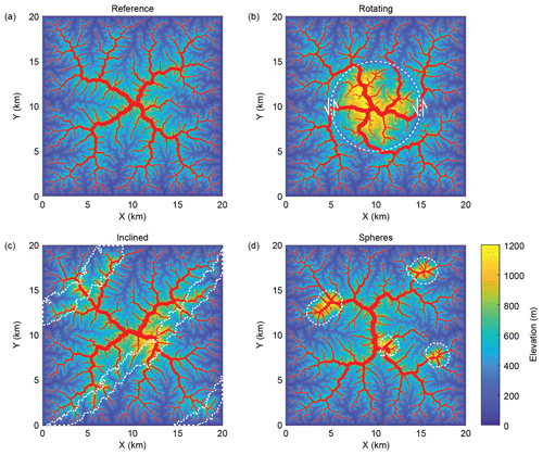
Figure 4Modeled topography and drainage divide network (red solid lines) at the end of the landscape evolution experiments: (a) Reference, (b) Rotating, (c) Inclined, and (d) Spheres. White stippled lines show strike-slip fault in panel (b) and regions with reduced erodibility in panels (c) and (d).
3.1 General behavior
The simulated landscapes, along with their drainage divide networks at the end of the numerical experiments, are shown in Figs. 4 and 5, and in the “Video supplement” (Scherler and Schwanghart, 2020b) we provide movies of all simulations. To provide a measure of the mobility of drainage divides, we computed the percentages of drainage area that were exchanged during the simulations between individual catchments that drain to the margin of the model domain (Fig. 6). Except for the Reference model, all models are characterized by notable changes in drainage area and mobile drainage divides. Area changes in the Initialize model are large in the beginning but level off rapidly during the first 1 Myr. Although area changes are small after 1 Myr, they continue for another 20 Myr, during which they are mostly decreasing. In the Rotating model, large area changes appear as discrete pulses induced by drainage captures of major streams (Fig. 5b), whereas the background area changes during rotation and faulting are relatively small (<0.1 % per 40 kyr). Area changes in the Inclined model are moderate (∼0.25 % per 40 kyr) throughout the simulation and oscillate in conjunction with the passage of more resistant layers through the landscape (Fig. 5c). Area changes in the Spheres model are generally more pronounced if the resistant spheres appear in the course of rivers, which forces them to steepen and to induce surface uplift upstream as opposed to their appearance at drainage divides, which increases the height of the divide but does not induce drainage divide migration at a larger scale (Fig. 5d).
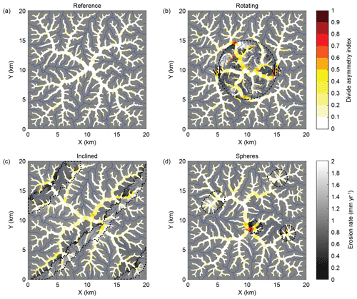
Figure 5Erosion rates and divide asymmetry index (DAI) at the end of the landscape evolution experiments: (a) Reference, (b) Rotating, (c) Inclined, and (d) Spheres. Black stippled lines show strike-slip fault in panel (b) and regions with reduced erodibility in panels (c) and (d).

Figure 6Changes in drainage area during the landscape evolution experiments. Y-axis unit is in percent per time step, which was 40 kyr.
3.2 Network topology
We first analyzed the response of the entire drainage network topology to the perturbations by quantifying the aggregated length of divide segments as a function of their order (Fig. 7). The first few million years of the Initialize model are characterized by large changes in divide lengths and orders. Initially, the divide network extends to orders as high as 100 but rapidly contracts as the drainage network becomes dendritic. After about 5 Myr, the highest orders are down to 60. Subsequent changes result in some scatter of the divide lengths but not in the range of divide orders. Compared to the Reference model, in which the divide network structure no longer changes, the Rotating, Inclined, and Spheres models exhibit changes in the divide network, mostly at divide orders greater than ∼20. This observation is related to the fact that low-order divides are distributed across the entire model domain and their number is accordingly high. Any of the perturbations we imposed only affect some of these divides, and thus the impact on their average length is rather small. In contrast, high-order divides are constrained to the highest parts of the modeled land surface and their numbers are much lower. The imposed perturbations typically affect a greater portion of them and hence the scatter in divide lengths is wider. In the Rotating and Spheres models, we also observed that maximum divide orders occasionally extend to higher values, but these changes are rather small. We note that the above observations also prevail when considering divide distance instead of divide order because the two are linearly related (Scherler and Schwanghart, 2020a), with divide distance ∼430 m × divide order. The 430 m corresponds to the mean length of the divide segments.
3.3 Topographic metrics
We next studied how the above-described disturbances affect drainage divide metrics during the simulations (Fig. 8). For all models, we computed the averages of the topographic parameters measured at drainage divides of specific divide distance intervals (Fig. 8a–d). As in the analysis of divide-segment lengths by order, it should be kept in mind that the numbers of divide segments, or their aggregated lengths (Fig. 7), are much higher for low orders and distances compared to higher ones. For reference, a divide order of 20 corresponds to a divide distance of approximately 9 km. In the Initialize model, all of the studied metrics attain a constant value that remains unchanged in the Reference model (Fig. 8) and that may or may not depend on the divide distance. For example, the mean elevation and junction connectivity (CJ) clearly increase with divide distance, whereas the flow distance exhibits only minor dependence on divide distance, and hillslope relief appears unrelated to divide distance. The dependency of some metrics on divide distance is partly explained by the model setup. Although divides with low distances also occur at higher elevation, the bulk of them are near the model edge, close to zero elevation. In contrast, divides at high distances are exclusively found near the center of the model, where elevations are also high. Similarly, the junction connectivity (CJ) is high in the model center, where the divides are far from most of the endpoints, which are more abundant near the edges of the model.
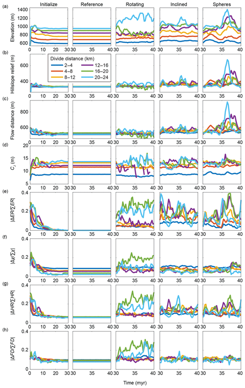
Figure 8Temporal evolution of the drainage divide network during the landscape evolution experiments. Colored curves show mean values for divide segments at different divide distances. (a) Elevation. (b) Hillslope relief (HR). (c) Flow distance (FD). (d) Junction connectivity (CJ). (e) Across-divide difference in erosion rate (). (f) Across-divide difference in chi (). (g) Across-divide difference in hillslope relief (), which is equal to the divide asymmetry index (DAI). (h) Across-divide difference in flow distance ().
It is also worth noting that none of the normalized across-divide differences in the topographic metrics attain zero values in the Reference model. This means that even at topographic steady state, there are residual across-divide differences in hillslope relief, flow distance, and χ. In the case of χ, these also depend on the divide distance and are greater closer to the model edge, where divide distances are low. In the perturbed models, we observed fluctuations in all topographic metrics, although of different magnitudes. For example, a comparison of across-divide differences in erosion rate with differences in hillslope relief, flow distance, and χ (Fig. 8e–h) shows that the normalized difference in hillslope relief (i.e., the divide asymmetry index) is sensitive to drainage divide mobility in all perturbed models, whereas across-divide differences in χ and flow distance are sensitive to divide mobility in the Rotating model but less so in the Inclined and Spheres models. The junction connectivity (CJ) metric attains temporally averaged values in the perturbed models that are quite similar to the constant values in the Reference model. In many cases, the deviations from the Reference model are greater the higher up in the divide network, i.e., for higher divide distances. This pattern is particularly visible in the Inclined model, wherein the amplitudes of the oscillations in all of the parameters increase with divide distance.
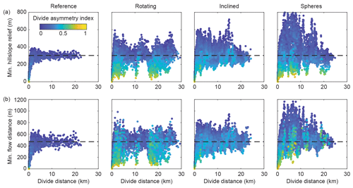
Figure 9Minimum hillslope relief (a) and minimum flow distance (b) of all divide segments along the drainage divide network from the last 1 Myr of the landscape evolution experiments Reference, Rotating, Inclined, and Spheres. Colors denote the divide asymmetry index (DAI). The black stippled line indicates the average values of minimum hillslope relief and minimum flow distance from the model Reference, measured between a divide distance of 10 and 20 km.
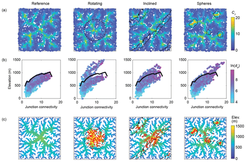
Figure 10Divide junction connectivity (CJ) from the final stage of the landscape evolution experiments Reference, Rotating, Inclined, and Spheres. CJ was calculated with a dd,max value of 5000 m. (a) Map view of divide junction CJ values. Black dashed lines indicate perturbation elements in the models. (b) Scatter plot of CJ by elevation, colored by the natural logarithm of the divide distance (dd). The thick black line follows the upper boundary of the divide junctions in the Reference model. (c) Drainage divide network colored by elevation. Red dots correspond to junctions in the perturbed models that lie higher than the junctions in the Reference models.
3.4 Minimum hillslope relief and flow distance
Motivated by the observation of constant values in hillslope relief and flow distance in the Reference model, as well as in actual landscapes (Scherler and Schwanghart, 2020a), and by our expectation that small values in either one would be found where one catchment loses area to another (Fig. 1), we next compared how minimum hillslope relief (HRmin), minimum flow distance (FDmin), and the divide asymmetry index (DAI) vary with divide distance in the Reference model and the three models with landscape perturbances (Fig. 9). In contrast to the average values in Fig. 8, we provide these metrics for all divide edges during the last 1 Myr of the model runs. Note also that we plotted data points in an order that brings high DAI values to the front to better assess where asymmetric divides are located, but in all four models, relatively high DAI points may plot on top of low DAI points. In the Reference model, both minimum hillslope relief and minimum flow distance reach relatively steady values (HRmin ∼250–350 m; FD–600 m) at a divide distance of ∼5 km. At lower divide distances, both HRmin and FDmin approach zero – simply because divides are defined to start at the stream network – and these divides can become increasingly more asymmetric. It is notable, however, that some of the highest HRmin and FDmin values are also observed at low divide distances of approximately 1–2 km. In the three other models, the transition between quite variable divides at short distances and more steady “background” values at higher distances appears to be preserved, but we observe generally more variability. For example, in the Rotating model, we observe divides with significantly lower HRmin and FDmin values at higher distances. These divides are particularly prominent at a distance of ∼10 and ∼15–22 km and correspond to the position of the strike-slip fault. Where HRmin and FDmin are low, DAI values are relatively high (divides are highly asymmetric), although there are also divides that have high DAI but regular HRmin and FDmin values. In the Inclined and Spheres models, the HRmin and FDmin values are never as low as in the Rotating model at divide distances >5 km, which reflects the lack of drainage captures. Instead, we observe frequent excursions to both higher and lower HRmin and FDmin values, either across all divide distances (Inclined) or at specific locations (Spheres). Deviations from the average values in the Reference model are greatest in the Spheres model compared to all other perturbed models and always correspond to peaks that grow where strong spheres are exhumed. In the three disturbance models, DAI values are generally higher than in the Reference model – although divides with high HRmin and FDmin values and at great divide distances mostly appear to have somewhat lower DAI values.
3.5 Junction connectivity
The spatial pattern of divide junction connectivity (CJ) values at the end of the landscape evolution experiments (Fig. 10) partly follows the pattern of divide distances (Fig. 4). Junctions with higher CJ values tend to occur at higher elevation and at greater divide distance (dd). In the Reference model, the highest CJ values occupy the center of the model domain and the centers of the four quadrants of the model domain, resembling the five on six-sided dice. In the Rotating model, these clusters of high CJ values are maintained, but their connection is disrupted by the strike-slip fault, which induces low CJ values. The centrally located divide junctions occupy a similar range in CJ values but are all shifted to higher elevations (Fig. 4). Similar, although lower, offsets to higher elevations occur in the Inclined and Spheres models, where junctions coincide with rocks of reduced erodibility. In the Spheres model, the basic structure of CJ values is similar to that of the Reference model, but the highest CJ values are steered towards the less erodible spheres, whereby they also attain CJ values that are distinctly higher than in any of the other models (Fig. 10b). In general, divide junctions with combinations of elevation and CJ values that are outside the range of values observed in the Reference model are found in the most disturbed parts of the landscape (Fig. 10c). In summary, the perturbed models appear to induce mostly changes in junction elevation, whereas changes in junction connectivity (CJ) are seemingly constrained to the Spheres model.
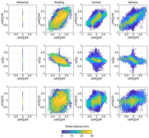
Figure 11Relationship between across-divide differences in the topographic metrics hillslope relief (HR), chi (χ), and flow distance (FD), with across-divide differences in erosion rates (ERs) for all divide edges in the last 1 Myr of the landscape evolution experiments Reference, Rotating, Inclined, and Spheres. Marker color denotes the divide distance (dd). Note that the markers are sorted by their divide distance to show the highest divide distance above data points with lower divide distance, and data points with lower divide distance occur beneath those with higher divide distance.
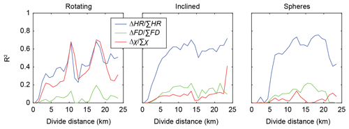
Figure 12Coefficient of determination for linear regressions between normalized across-divide differences in different topographic metrics (HR: hillslope relief; FD: flow distance; χ: chi) and normalized across-divide differences in erosion rates as a function of drainage divide distance in the three perturbation models.
4.1 Quantifying drainage divide mobility
The analysis of stream networks has become a standard tool for inferring tectonic forcing and landscape history (e.g., Wobus et al., 2006; Kirby and Whipple, 2012; Demoulin, 2012; Schwanghart and Scherler, 2014). The divide network holds the potential to record similar tectonic forcing, but also other aspects of landscape history (e.g., Willett et al., 2014). The question is which divide metrics are useful to analyze, and what do they tell us about landscape history? Our Rotating model induced relatively sudden drainage captures (Fig. 6). Because such events are associated with the dissection of drainage divides, reliable indicators are values of hillslope relief (HR) and flow distance (FD) that are much lower compared to the values that divides ( km divide distance) strive for (Fig. 9). More gradual divide migration, however, likely lacks such simple diagnostic criteria, and in those cases, across-divide differences in topographic metrics may be more suitable indicators of divide mobility. The most commonly used metric to infer drainage divide mobility is the across-divide difference in χ (Willett et al., 2014). Although the utility of this metric has recently received some critique (Whipple et al., 2017b; Forte and Whipple, 2018), it has become a popular tool for studying drainage divides. Whipple et al. (2017b) and Forte and Whipple (2018) instead advocated the use of other topographic metrics, including mean gradient, mean local relief, and channel bed elevation, measured at or upstream of a reference drainage area. We note that these latter metrics are typically highly correlated and very similar to the hillslope relief and DAI metrics that we included in this study.
Figure 11 shows how normalized across-divide differences in χ, hillslope relief (HR), and flow distance (FD) compare to normalized across-divide differences in erosion rate (ER), evaluated for each divide edge from the last 1 Myr of the landscape evolution experiments Reference, Rotating, Inclined, and Spheres. We find that across-divide differences in hillslope relief (HR; Fig. 11a) are most sensitive to the disturbances included in the models, whereas across-divide differences in χ are similarly sensitive to disturbances in the Rotating model but less so in the Inclined and Spheres models (Figs. 11b, 8). Across-divide differences in flow distance (FD) are the least sensitive to disturbances in the models and show the largest scatter when compared with erosion rates (Fig. 11c). However, there is also substantial scatter in the relationship between across-divide differences in hillslope relief and erosion rate, which partly depends on the divide distance. In general, we observe that the scatter is higher for divide distances km (dark blue in Fig. 11), which corresponds to the value below which we observe large variability in divide morphology, even in the Reference model (Fig. 9). To quantify the correlation of the normalized across-divide differences in topographic metrics with normalized across-divide differences in erosion rate, we fitted a linear model to all drainage divide edges from the entire model runs, categorized into 1 km divide distance bins, and show the resulting coefficients of determination (R2) in Fig. 12. As already suspected from Figs. 8 and 11, the R2 values differ between models and metrics and also depend on divide distance. In general, we observe that all metrics perform poorly at divide distances km and that across-divide differences in flow distance perform poorly even at higher distances. The highest R2 values are linked to across-divide differences in hillslope relief, whereas across-divide differences in χ attain similar R2 values in the Rotating model but some of the lowest R2 values of all metrics in the Inclined and Spheres model. This difference may be explained by the fact that in the latter two models, we introduced spatial variability in the erosional efficiency of rivers (Kr) that we did not account for in our across-divide comparison of χ, as would be required (Willett et al., 2014). In natural landscapes, however, these values and their variability are rarely well known.
We speculate that the influence of divide distance on topographic metric–erosion rate relationships may also account for the differences in scatter observed by Sassolas-Serrayet et al. (2019) in landscape evolution experiments similar to our Initialize model between larger and smaller basin areas. But even when excluding divides of low order or low divide distance, we still observe considerable scatter in the topographic metric–erosion rate relationships, which, at the very least, demands caution when interpreting divide morphology in terms of mobility. In this regard, studying Fig. 5 and the videos of the landscape evolution experiments (see the “Video supplement”; Scherler and Schwanghart, 2020b) is insightful: where drainage divides are migrating, one typically observes a range of across-divide topographic metric values that vary considerably during the migration. In other words, despite a continuous divide migration at a large scale, there is often small-scale variability in divide morphology that may in part be related to across-divide differences in topographic metrics lagging behind across-divide differences in erosion rate.
As a final note, we emphasize that the above observations are from our numerical experiments, which depict an idealized world. It is clear that the complexities present in nature, such as anisotropic and variable rock properties, hydroclimatic gradients, mass-wasting events, and biological influences on erosion processes and rates, can lead to landscape patterns that bias any of the above topographic metrics and need to be taken into account when inferring divide dynamics from divide metrics in natural landscapes.
4.2 Divide network dynamics
Stream networks tend to attain configurations that are in equilibrium with the geological and climatic environment, given an initial condition (e.g., Rinaldo et al., 2014). Because drainage divides are defined by adjacent drainage basins, the geometry of divide networks should attain a similar equilibrium, which expresses itself in both the geometry of divides and the topology of divide networks. Our numerical experiments have shown that during the initial establishment of a stream network, on a relatively flat surface, both stream and divide networks are far from their steady-state configuration and characterized by networks that extend to high orders (Fig. 7) and long divide distances. During the subsequent extension and shrinkage of individual streams towards their steady-state configuration, the divide network contracts and primarily high-order divide segments shorten and become fewer, whereas divides of low orders maintain their frequencies (Fig. 7).
In general, divide segments of high order, i.e., at great distance from endpoints, appear to be the most responsive to landscape disturbances (Fig. 8). In the case of the Rotating model, this is in part expected because the inner rotating part of the landscape contains the highest-order divide segments (Fig. 4b). In the cases of the Inclined and Spheres models, it may be related to the increased probability of recording a disturbance because the adjoining basins cover a larger area compared to lower-order divides. In other words, if drainage captures happen somewhere within a drainage basin, this will most likely influence divides further upstream. Over a distance of less than ∼5 km from divide network endpoints, the divide segments transition from low interfluves at river junctions to high topographic ridges, as seen in the Reference model (Fig. 9). In the other models, most of the investigated morphometric parameters are quite variable over the same distance and can be seen to rapidly adjust to disturbances such as drainage captures or migrating divides. Such behavior is consistent with the observation that the timescale of a river's response to changes in drainage area increases with the distance from the divide to the outlet of a river (Whipple et al., 2017b). To reliably distinguish the morphologic effects of real disturbances from “noise” close to the river, a minimum divide distance of perhaps ∼5 km, as in our analysis of the Big Tujunga divide network (Scherler and Schwanghart, 2020a), appears appropriate. This minimum divide distance could be lower or higher, depending on factors like drainage density and average hillslope relief, for example.
Our new junction connectivity index (CJ) complements existing topographic metrics in assessing divide network dynamics. For example, the junction connectivity in our Rotating model is low along the fault (Fig. 10), consistent with the absence of stable divides. In the Spheres model, however, the appearance of more resistant rocks at the surface often resulted in the migration of divides towards the spheres (Fig. 5c, “Video supplement”; Scherler and Schwanghart, 2020b). In this case, parts of the drainage divide network were mobile, not stable, but they moved towards particularly stable portions in the landscape. Therefore, the junction connectivity index (CJ) may also be interpreted as an attractor or centrality index (Phillips et al., 2015) that quantifies how strong a drainage divide network has been pulled towards and anchored at a certain junction (Spotila, 2012).
Based on landscape evolution model experiments in which we forced divides to migrate, we found that stable drainage divides strive to attain a constant hillslope relief and flow distance from the nearest stream, provided a sufficiently large divide distance to avoid confounding influences near the edges of the divide network. In our experiments this distance is ∼5 km from endpoints. Simple indicators of mobile divides are anomalously low hillslope relief or flow distance values, which could signal beheaded valleys or future capture events. Overall, drainage divides located high up in the network, i.e., at great distance from endpoints, are more vulnerable than divides closer to endpoints of the network and are more likely to record disturbance for a longer time period. In our comparison of different topographic metrics to assess drainage divide mobility, we found that across-divide differences in hillslope relief proved more useful for assessing divide migration than other tested metrics.
The divide algorithm developed in Scherler and Schwanghart (2020a) has been implemented in the TopoToolbox v2 (Schwanghart and Scherler, 2014). The codes will be made available with the next TopoToolbox release and shall be accessible at https://github.com/wschwanghart/topotoolbox (last access: 17 April 2020).
The “Video supplement” related to this article is available online at https://doi.org/10.5880/GFZ.3.3.2019.005 (Scherler and Schwanghart, 2020b).
DS conducted the modeling and led the writing of the paper. Both authors contributed to discussions, editing, and revising the paper.
The authors declare that they have no conflict of interest.
We thank two anonymous reviewers for constructive comments that helped improve the paper.
This research has been supported by the Deutsche Forschungsgemeinschaft (DFG; grant no. SCHE 1676/4-1).
The article processing charges for this open-access
publication were covered by a Research
Centre of the Helmholtz Association.
This paper was edited by Sebastien Castelltort and reviewed by two anonymous referees.
Braun, J. and Sambridge, M.: Modelling landscape evolution on geological time scales: a new method based on irregular spatial discretization, Basin Res., 9, 27–52, https://doi.org/10.1046/j.1365-2117.1997.00030.x, 1997.
Campforts, B., Schwanghart, W., and Govers, G.: Accurate simulation of transient landscape evolution by eliminating numerical diffusion: the TTLEM 1.0 model, Earth Surf. Dynam., 5, 47–66, https://doi.org/10.5194/esurf-5-47-2017, 2017.
Castelltort, S., Goren, L., Willett, S. D., Champagnac, J. D., Herman, F., and Braun, J.: River drainage patterns in the New Zealand Alps primarily controlled by plate tectonic strain, Nat. Geosci., 5, 744–748, https://doi.org/10.1038/ngeo1582, 2012.
Clark, M. K., Schoenbohm, L., Royden, L. H., Whipple, K. X., Burchfiel, B. C., Zhang, X., Tang, W., Wang, E., and Chen, L.: Surface uplift, tectonics, and erosion of eastern Tibet as inferred from large-scale drainage patterns, Tectonics, 23, TC1006, https://doi.org/10.1029/2002TC001402, 2004.
Clift, P. D., Blusztajn, J., and Duc, N. A.: Large-scale drainage capture and surface uplift in eastern Tibet–SW China before 24 Ma inferred from sediments of the Hanoi Basin, Vietnam, Geophys. Res. Lett., 33, L19403, https://doi.org/10.1029/2006GL027772, 2006.
Culling, W. E. H.: Soil Creep and the Development of Hillside Slopes, J. Geol., 71, 127–161, https://doi.org/10.1086/626891, 1963.
Demoulin, A.: Morphometric dating of the fluvial landscape response to a tectonic perturbation, Geophys. Res. Lett., 39, L15402, https://doi.org/10.1029/2012GL052201, 2012.
Duvall, A. R. and Tucker, G. E.: Dynamic Ridges and Valleys in a Strike-Slip Environment, J. Geophys. Res.-Earth, 120, 2016–2026, https://doi.org/10.1002/2015JF003618, 2015.
Forte, A. M. and Whipple, K. X.: Criteria and tools for determining drainage divide stability, Earth Planet. Sc. Lett., 493, 102–117, https://doi.org/10.1016/j.epsl.2018.04.026., 2018.
Howard, A. D. and Kerby, G.: Channel changes in badlands, Geol. Soc. Am. Bull., 94, 739–752, https://doi.org/10.1130/0016-7606(1983)94<739:CCIB>2.0.CO;2, 1983.
Kirby, E. and Whipple, K. X.: Expression of active tectonics in erosional landscapes, J. Struct. Geol., 44, 54–75, 2012.
O'Hara, D., Karlstrom, L., and Roering, J. J.: Distributed landscape response to localized uplift and the fragility of steady state, Earth Planet. Sc. Lett., 506, 243–254, https://doi.org/10.1016/j.epsl.2018.11.006, 2018.
Perron, J. T. and Royden, L. H.: An integral approach to bedrock river profile analysis, Earth Surf. Proc. Land., 38, 570–576, https://doi.org/10.1002/esp.3302, 2013.
Phillips, J. D., Schwanghart, W., and Heckmann, T.: Graph theory in the geosciences, Earth-Sci. Rev., 143, 147–160, https://doi.org/10.1016/j.earscirev.2015.02.002, 2015.
Rinaldo, A. Rigon, R., Banavar, J. R., Maritan, A., and Rodriguez-Iturbe, I.: Evolution and selection of river networks: Statics, dynamics, and complexity, P. Natl. Acad. Sci. USA, 111, 2417–2424, https://doi.org/10.1073/pnas.1322700111, 2014.
Sassolas-Serrayet, T., Cattin, R., Ferry, M., Godard, V., and Simoes, M.: Estimating the disequilibrium in denudation rates due to divide migration at the scale of river basins, Earth Surf. Dynam., 7, 1041–1057, https://doi.org/10.5194/esurf-7-1041-2019, 2019.
Scherler, D. and Schwanghart, W.: Drainage divide networks – Part 1: Identification and ordering in digital elevation models, Earth Surf. Dynam., 8, 245–259, https://doi.org/10.5194/esurf-8-245-2020, 2020a.
Scherler, D. and Schwanghart, W.: Drainage divide networks, Part 2: Response to perturbations – Supplementary movie files. https://doi.org/10.5880/GFZ.3.3.2019.005, 2020b.
Schwanghart, W. and Scherler, D.: Short Communication: TopoToolbox 2 – MATLAB-based software for topographic analysis and modeling in Earth surface sciences, Earth Surf. Dynam., 2, 1–7, https://doi.org/10.5194/esurf-2-1-2014, 2014.
Spotila, J. A.: Influence of drainage divide structure on the distribution of mountain peaks, Geology, 40, 855–858, 2012.
Whipple, K. X. and Tucker, G. E.: Dynamics of the stream-power river incision model: Implications for height limits of mountain ranges, landscape response timescales, and research needs, J. Geophys. Res.-Sol. Ea., 104, 17661–17674, https://doi.org/10.1029/1999JB900120, 1999.
Whipple, K. X., DiBiase, R. A., Ouimet, W. B., and Forte, A. M.: Preservation or piracy: diagnosing low-relief, high-elevation surface formation mechanisms, Geology, 45, 91–94, https://doi.org/10.1130/G38490.1, 2017a.
Whipple, K. X., Forte, A. M., DiBiase, R. A., Gasparini, N. M., and Ouimet, W. B.: Timescales of landscape response to divide migration and drainage capture: implications for the role of divide mobility in landscape evolution. J. Geophys. Res.-Earth, 122, 248–273, https://doi.org/10.1002/2016JF003973, 2017b.
Willett, S. D., McCoy, S. W., Perron, J. T., Goren, L., and Chen, C. Y.: Dynamic reorganization of river basins, Science, 343, 1248765, https://doi.org/10.1126/science.1248765, 2014.
Wobus, C. W., Whipple, K. X., Kirby, E., Snyder, N. P., Johnson, J., Spyropolou, K., Crosby, B. T., and Sheehan, D.: Tectonics from topography: Procedures, promise, and pitfalls, in: Tectonics, climate, and landscape evolution, edited by: Willett, S. D., Hovius, N., Brandon, M. T., and Fisher, D., 398, 55–74, The Geological Society of America, Boulder, CO, USA, 2006.
Yang, R., Willett, S. D., and Goren, L.: In situ low-relief landscape formation as a result of river network disruption, Nature, 520, 526–529, https://doi.org/10.1038/nature14354, 2015.


