the Creative Commons Attribution 4.0 License.
the Creative Commons Attribution 4.0 License.
 | 10 Sep 2021
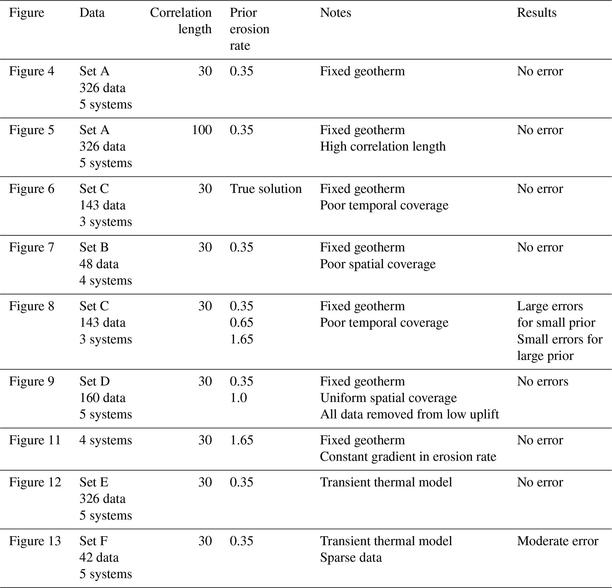
Bias and error in modelling thermochronometric data: resolving a potential increase in Plio-Pleistocene erosion rate
Sean D. Willett
Frédéric Herman
Matthew Fox
Nadja Stalder
Todd A. Ehlers
Ruohong Jiao
Rong Yang
Thermochronometry provides one of few methods to quantify rock exhumation rate and history, including potential changes in exhumation rate. Thermochronometric ages can resolve rates, accelerations, and complex histories by exploiting different closure temperatures and path lengths using data distributed in elevation. We investigate how the resolution of an exhumation history is determined by the distribution of ages and their closure temperatures through an error analysis of the exhumation history problem. We define the sources of error, defined in terms of resolution, model error and methodological bias in the inverse method used by Herman et al. (2013) which combines data with different closure temperatures and elevations. The error analysis provides a series of tests addressing the various types of bias, including addressing criticism that there is a tendency of thermochronometric data to produce a false inference of faster erosion rates towards the present day because of a spatial correlation bias. Tests based on synthetic data demonstrate that the inverse method used by Herman et al. (2013) has no methodological or model bias towards increasing erosion rates. We do find significant resolution errors with sparse data, but these errors are not systematic, tending rather to leave inferred erosion rates at or near a Bayesian prior. To explain the difference in conclusions between our analysis and that of other work, we examine other approaches and find that previously published model tests contained an error in the geotherm calculation, resulting in an incorrect age prediction. Our reanalysis and interpretation show that the original results of Herman et al. (2013) are correctly calculated and presented, with no evidence for a systematic bias.
- Article
(93088 KB) - Full-text XML
- BibTeX
- EndNote


Thermochronometry provides one of few methods to quantify rock exhumation histories. Over the last 30 years, it has been extensively applied to understand tectonics and landscape evolution. Part of its success stems from the large number of thermochronometer systems available (Reiners and Brandon, 2006; Reiners et al., 2005) as well as the development of numerical models able to convert thermochronometric data into constraints on cooling associated with exhumation by surface or tectonic processes (e.g. Braun, 2003; Ehlers and Farley, 2003; Ketcham, 2005; Gallagher, 2012; Braun et al., 2012; Willett and Brandon, 2013; Fox et al., 2014). Where exhumation occurs by surface processes, the exhumation rate is equivalent to a surface erosion rate, and we will use these two terms interchangeably in this paper. Models are an integral part of thermochronometric data interpretation as they are needed for computing cooling histories from parent–daughter loss relationships with a complex thermal history as well as for converting cooling histories into exhumation histories. Cooling or exhumation histories provide direct constraints on kinematics or tectonic processes and rates of surface erosional processes (e.g. Grasemann and Mancktelow, 1993; Seward and Mancktelow, 1994; Brandon et al., 1998; Batt et al., 2000; Moore and England, 2001; Willett and Brandon, 2002; Ehlers et al., 2003; Lock and Willett, 2008; Campani et al., 2010; Herman et al., 2010; Barnes et al., 2012; McQuarrie and Ehlers, 2015).
Surface erosional processes are closely linked to climate through parameters and processes such as temperature, precipitation and biological activity (e.g. Antonelli et al., 2018; Starke et al., 2017). Temperature determines the dominant surface processes, for example glacial, fluvial or hillslope, and precipitation often determines efficiency as well as its spatial distribution. Thermochronometry holds the potential to provide a measure of past erosional conditions and therefore how these conditions may be related to past climate and how the coupled system has evolved (e.g. Shuster et al., 2005, 2011; Burbank et al., 2003; Reiners et al., 2003; Wobus et al., 2003; Vernon et al., 2008; Thomson et al., 2010a; Thiede and Ehlers, 2013; Fox et al., 2015, 2016; Herman and Brandon, 2015).
One of the fundamental questions of paleoclimate and its links to Earth processes is how the onset of Quaternary glaciations affected solid Earth processes including surface erosional efficiency. Glaciers can be very efficient agents of surface erosion, and regions of heavy continental or Alpine glaciation have clearly been morphologically modified. Whether geomorphic change has a corresponding change in net erosion rates is a more difficult question, although support for a Quaternary increase in global erosion rate comes from sedimentological evidence (Molnar and England, 1990; Zhang et al., 2001; Molnar, 2004). A second open question is whether regions that have experienced Quaternary climate change but have remained too warm for active glaciation have also experienced an increase in average erosion rate, for example through increases in precipitation or climate variability (Zhang et al., 2001; Molnar, 2004). Controversy surrounds this question in part because many orogens experienced a decrease in precipitation in the Quaternary due to cooler air temperatures holding less moisture during glacial periods (e.g. Mutz et al., 2018; Mutz and Ehlers, 2019).
Although numerous single-site thermochronometry studies have shown increases in Pliocene or Quaternary erosion rates (e.g. Zeitler et al., 1982; Tippett and Kamp, 1993; Farley et al., 2001; Shuster et al., 2005, 2011; Berger and Spotila, 2008; Berger et al., 2008a, b; Vernon et al., 2008; Glotzbach et al., 2011; Valla et al., 2011, 2012; Sutherland et al., 2009; Thomson et al., 2010a, b; Avdeev and Niemi, 2011; Thiede and Ehlers, 2013; Fox et al., 2015, 2016; Michel et al., 2018), the first attempt to conduct a global-scale analysis was carried out by Herman et al. (2013). Herman et al. (2013) compiled about 17 000 thermochronometric ages from around the world primarily from four low-temperature thermochronometric systems, apatite and zircon (AHe and ZHe), and apatite and zircon fission track dating (AFT and ZFT). In some cases, they augmented these systems with higher closure temperature thermochronometers. These data were interpreted to quantify the exhumation rate history of select regions distributed globally. A key objective of that study was to apply a uniform treatment of the data using a transient thermal model embedded in a Bayesian inverse model (Fox et al., 2014). Using this approach, Herman et al. (2013) found that of sites that had enough thermochronometric data to resolve a recent change in erosion rate, over 80 % were dominated by an increase in erosion rate over the past 4 Myr. These sites included both tectonically active and inactive settings, glaciated and unglaciated regions and locations in the Northern Hemisphere and Southern Hemisphere. Although Herman et al. (2013) did not attempt to attribute cause to any single locality, they argued that the strong skew towards an increase in erosion rate at such varied localities supported a common global phenomenon most likely related to climate change (Zhang et al., 2001). The spatial extent of regions directly sampled by thermochronometry with sufficient resolution to establish a change in erosion rate was very small (Herman et al., 2013, Fig. 3). Furthermore, these sites are biased to areas with high erosion rates given that resolution of rate changes over the last 5 Ma requires that thermochronometers exhibit ages under 5 Ma. Herman et al. (2013) were explicit in their conclusions that their results do not provide an estimate of either modern global erosion rate or past global rates, but rather they provided a measure of how rates have changed over the last ca. 5 Ma in these local high erosion rate regions. The fact that sites included a large number of mid-latitude mountain regions with evidence for Quaternary glaciations is circumstantial support that glacial erosion has contributed to this result, but this was not claimed to be proven by Herman et al. (2013).
However, a recent paper by Schildgen et al. (2018) challenged these conclusions, arguing that the Bayesian inversion method employed by Herman et al. (2013) incorrectly interpreted spatial variability as temporal variability, resulting in a systematic bias towards an apparent temporal acceleration in exhumation. This contention not only suggests that the conclusions of Herman et al. (2013) are incorrect, but also calls into question the results of numerous other studies using the same method.
The objective of this paper is to test the hypothesis of recent work suggesting the interpretations of Herman et al. (2013) contain a bias. We test this hypothesis by conducting a complete error analysis of the method of Herman et al. (2013). The current paper is structured into three main parts. First, we provide a review of concepts associated with bias and resolution inherent to thermochronometry as well as to methods of data treatment, including the method proposed by Herman et al. (2013) and Fox et al. (2014) (Sects. 2 and 3). This is necessary to explain potential sources of error and how to test for them. Second, we conduct a series of tests based on synthetic data and a specified and therefore known erosion rate history in order to isolate and identify the sources and magnitudes of errors (Sect. 4). Third, we conduct an interpretation and assessment of selected examples from the original Herman et al. (2013) results in order to explain which data were responsible for resolving the various erosion rate histories and how these were averaged in space and time (Sect. 5). Finally, we review the analysis of Schildgen et al. (2018) to identify the source of discrepancies between their results and the findings of this paper. We determine that Schildgen et al. (2018) made a series of self-reinforcing errors that combined to create the appearance of a widespread bias in the original analysis of Herman et al. (2013) that does not exist.
2.1 Resolution of erosion rate from thermochronometric ages
The problem of determining an exhumation history from thermochronometric ages is relatively simple. Expressed in terms of a closure temperature, Tc, which is an approximation to temperature-dependent diffusional loss of a daughter product, and knowing the geotherm, T(z), the rate of exhumation, or erosion rate, e, can be expressed as
where τ is the measured age and zc is the depth to the closure temperature below a sample in one dimension. Complications to this approach arise from transient geotherms and the cooling rate dependence of the closure temperature (e.g. Graseman and Mancktelow, 1993; Mancktelow and Grasemann, 1997; Batt and Braun, 1997; Harrison et al., 1997; Moore and England, 2001; Braun et al., 2006; Reiners and Brandon, 2006; Willett and Brandon, 2013), but the principle holds for most cases of monotonic cooling. A single age can resolve only a single rate of cooling between its time of closure and sampling at the surface. Resolving more complex (e.g. transient) exhumation histories requires more information.
Several methods have been proposed for calculation of either cooling rates or exhumation rates from thermochronometric data. The simplest method is by using the relationship between age and elevation (Fig. 2a) (Wagner and Reimer, 1972; Wagner et al., 1979; Parrish, 1983; Fitzgerald and Gleadow, 1988; Fitzgerald et al., 1995). This relationship exploits the fact that path length from the depth of closure to the surface increases with elevation. Provided that the closure isotherm is horizontal and the exhumation rate is spatially constant over the sampling domain, the relationship is monotonic, with the slope giving the exhumation rate. Sampling across elevation also requires sampling horizontally, so an important assumption is that sample points are closely located in space, typically within a few kilometres of each other, so that exhumation rates and the depth to the closure isotherm do not differ between points. Application of this method also requires that surface relief has not significantly perturbed the depth to the closure isotherm (e.g. Lees, 1910; Stüwe et al., 1994; Mancktelow and Graseman, 1997; Braun, 2002a, b; Ehlers, 2005).
The second method for estimating exhumation rate is by calculation of a cooling rate using more than one thermochronometric system (e.g. Harrison et al., 1979; Dodson and McClelland-Brown, 1985; Hurford, 1986). This method has a long history of use for metamorphic cooling histories in orogenic belts, where it is referred to as the two-mineral or mineral-pair method and has identical application to low-temperature systems and erosional cooling to the surface. By using two thermochronometric systems and taking the difference between closure temperatures and ages, one can calculate a cooling rate (Fig. 2b). To convert the cooling rate to an exhumation rate requires a thermal model or knowledge of the geotherm, and if the geotherm is not linear, variations in cooling rate may not have corresponding changes in exhumation rate. For example, if the geotherm is convex upward due to upward advection of heat, a constant rate of exhumation may manifest itself as an increase in cooling rate as rock nears the surface. Cooling rates should thus never be directly converted to exhumation rates without considering variations in the thermal gradient with depth (Moore and England, 2001). Different closure temperatures are used to resolve the time taken to pass from one closure depth to another or from the shallowest closure depth to the surface (Reiners and Brandon, 2006) (Fig. 2b).
Resolution of an exhumation rate history from thermochronometric ages is thus determined by the range of ages, the number and range of the closure temperature and the distribution of elevation of samples (Fig. 1). This description of resolution differs from other problems in parameter estimation in that the resolution is determined by the value measured, i.e. the age, in addition to the location of a measurement. The estimation problem is to determine an exhumation rate in both space and time. However, the ages measured at a particular point in space determine how much time can be resolved and the number of thermochronometers combined with the elevation distribution determine how many time intervals can be resolved.
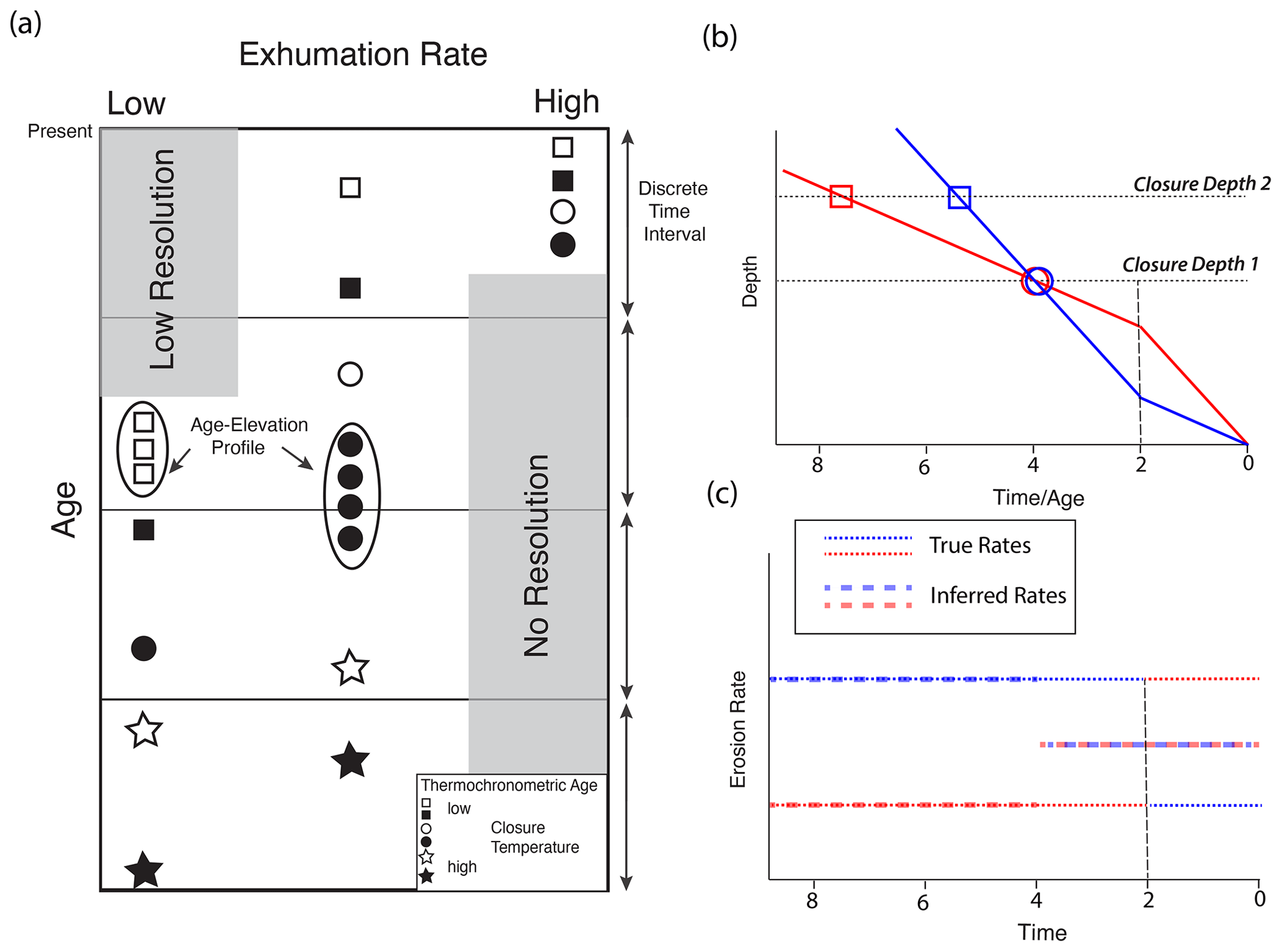
Figure 1(a) Illustration of how the distribution of thermochronometric ages constrains exhumation rate in time and for different exhumation rates. Discrete time intervals as used in an inverse model are indicated. Hypothetical ages are shown for six thermochronometer systems with different closure temperatures. Age–elevation relationships extend the age range for a single thermochronometer as shown by ellipses enclosing samples with the same symbol. Note that there is no resolution for times greater than the oldest age at a site. For time intervals younger than the youngest age, only a single (low-resolution) time interval can be resolved. (b) Example of how erosion rate is estimated over an unsampled time interval through the use of older ages. Assumed change in rate at 2 Ma with the youngest age being 4 Ma. Red curve is for an increase in rate; blue curve is for a decrease. (c) Inferred erosion rates using the two-mineral method. Note that the change in each case is underestimated but still detected.
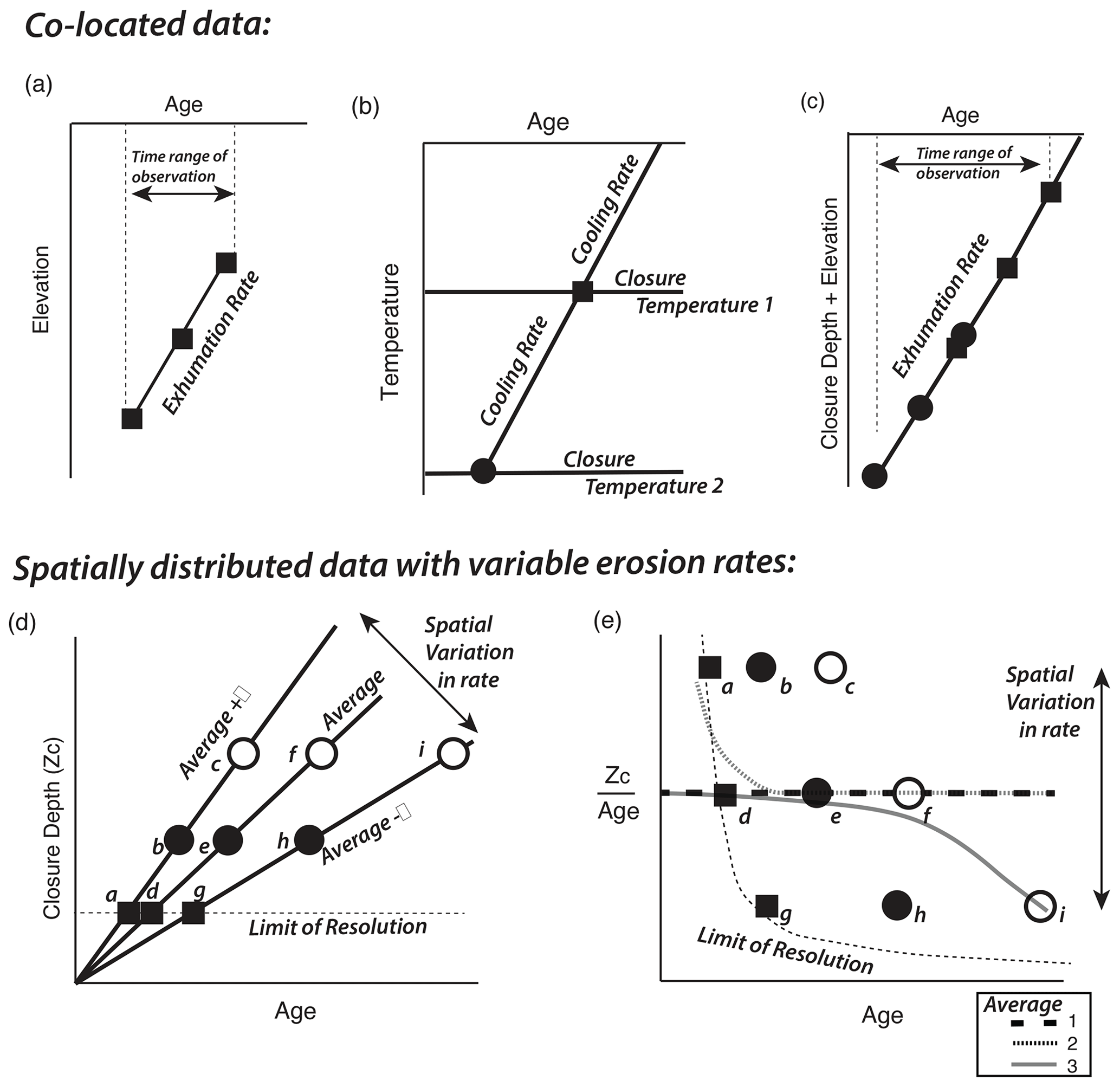
Figure 2Methods for combining thermochronometric ages with variability due to spatial variations in exhumation rate or elevation. Squares and circles represent thermochronometers from independent systems as in Fig. 1. (a) Plot of age against elevation for three, effectively co-located data. Slope is an estimate of exhumation rate. (b) Multi-thermochronometer method for determining exhumation rate over two intervals by measuring cooling rate between time of passage of closure temperature. (c) Combining elevation and multi-thermochronometer methods, using a thermal model to calculate closure depths. (d) Hypothetical age distribution for three thermochronometers across a region including three spatial domains with different exhumation rates. Exhumation rates are at the regional average and at plus or minus some deviation, σ, from the average. Limit of resolution shows the age below which no change in exhumation rate can be resolved. (e) Several proposed methods for averaging the ages of (d) to produce an exhumation rate. “Average 1” represents the average rate of all nine ages and is an unbiased estimate of the regional median rate. Average 1 is also obtained by taking the median age for each closure temperature and converting this to a rate. “Average 2” is obtained by averaging only the ages that fall within a specific time window. “Average 3” is obtained by averaging the rates from all ages older than a specific time. Methods in (a)–(c) and “Average 1” in (e) are unbiased estimates of local or regional median exhumation rate, although the resolved time span varies. Averaging methods 2 and 3 in (e) are biased, although over different time spans.
The integral nature of thermochronometric data (Eq. 1) implies that even time intervals without ages are sampled, if not fully resolved. For example, the “low-resolution” region of Fig. 1a contains no young ages within the interval, but the older ages at that location constrain the erosion rate over the last time interval. To illustrate this, Fig. 1b and c show an example of how a change in erosion rate at 2 Ma would still be resolved by a 4 Ma age combined with older ages and using the two-mineral method. Without ages falling directly on the time of a change in rate, the change is not precisely resolved, but it is still detected. In this example, a 4 Ma age would detect an increase or a decrease in erosion rate but with half (ignoring the non-linear relationship between age and erosion rate) the magnitude and spread over time.
A third method for determining a cooling or exhumation rate uses a thermal model that calculates the thermal history of exhumed rocks by solving the advection–diffusion equation for prescribed parameters (e.g. rate of exhumation, thermophysical properties, and boundary and initial conditions). Application of a thermal model permits estimation of the geotherm including depths to closure temperatures, and with this information, single ages (Willett and Brandon, 2013) or multiple ages with elevations can be combined into a single equivalent of an age–elevation relationship, greatly increasing the time span and details of the exhumation history resolved by data (Fig. 2c) (Reiners and Brandon, 2006).
2.2 Spatial correlation bias
In order to increase the applicability of thermochronometers, it is necessary to amalgamate data spatially. Even an age–elevation profile is a collection of data across some spatial region. Important questions in these methods are over what distance is this valid, and are there unintended consequences to spatial averaging? In particular, it has been suggested that spatial variations in age can be mistakenly combined to produce an inference of temporal change. For example, if elevation and erosion rate covary over some region, amalgamating ages might produce a linear elevation trend but not one that reflects the average erosion rate. With spatial variation in erosion rates, it is possible to combine the ages in a way that would mimic an increase in erosion rate with time (Willenbring and Jerolmack, 2016; Schildgen et al., 2018). However, there are many ways in which thermochronometric ages can be averaged or combined to construct an erosion rate history, so it is important to evaluate methods to establish potential bias from specific assumptions.
To frame this problem, we show a thought experiment in Fig. 2d and e, similar to the one set up by Willenbring and Jerolmack (2016). Figure 2d shows ages from three thermochronometers exhumed at a constant rate and set at three different closure depths. We define three sets of ages, each of which experienced exhumation at a different rate: at the average rate and varying from the average by a value of σ but in opposite directions. These data can be regarded as coming from three regions, each exhuming at a different but steady rate. For simplification, we will keep the closure depth constant and assume no elevation differences for the ages, although a range in elevation is equivalent to independent closure temperatures. The ages define three lines; the slope of each gives the local exhumation rate (Fig. 2e). Willenbring and Jerolmack (2016) (their Fig. 3) defined a deviation in age rather than exhumation rate, but their example is otherwise equivalent.
There are many ways in which these data can be analysed and erosion rates derived, mostly depending on how much variability in the exhumation history one attempts to resolve and with what spatial resolution. If one recognizes that these data come from three independent areas, data from each area, i.e. a–c, d–f, or g–i, define an exhumation history that is steady in time, and any regression of age and depth to the closure isotherm gives the correct erosion rate value, with temporal resolution determined by how many data are available at each location. If one fails to recognize that these data have independent exhumation rates, they will be averaged, but there are many ways that this can be done. The simplest way is to average the rates from all nine points shown as “Average 1” in Fig. 2b. This gives an unbiased, i.e. correct, measure of the regional median erosion rate but with no time resolution. To resolve time variation requires averaging subsets of the data, for example by taking a regression of the data in Fig. 2d with a moving window or with a piecewise constant slope. Willenbring and Jerolmack (2016) argued that there is a limit to resolution at short times (shown as a fine dashed line in Fig. 2d and e), so that the region below this limit is unsampled. They calculated an average exhumation rate as the expected value of the measured rates, integrated at a fixed time but excluding the region below this limit; their average is shown as “Average 2” in Fig. 2e.
However, using a constant time window to average rates (Fig. 2d) or to regress closure depth against time (Fig. 2d) presents some statistical problems. Time is not the independent variable in this problem. The time information is entirely from measured thermochronometric ages, which makes time a dependent variable, so one should not regress depth against age. In fact, if one regresses age against depth (Fig. 2d) with a moving depth window, one obtains the correct, unbiased regional mean erosion rate (Fig. 2e, Average 1). Any change in the average erosion rate will be detected with resolution determined by the number of sampled closure depths.
A second aspect of this problem reflects the fact that thermochronometric data represent an integral quantity, namely the integral of the exhumation rate (Eq. 1) from the time of closure to the present day. As such, a moving window in time that includes only ages that fall into that window (Average 2) does not include the constraint provided by the older ages. For this reason, Average 2 in Fig. 2 has, to our knowledge, never been used in thermochronometry studies, and methods such as that of Herman et al. (2013) that are based on the integral as shown in Eq. (1) do not default to this condition.
Recognizing the integral nature of a thermochronometric age, all data older than a time of interest should be included in the determination of the rate across that interval. Applying this method gives Average 3 in Fig. 2e. This average is unbiased at younger times. If there is an upper limit to the closure temperatures or elevation, the average is biased for early times that are undersampled at high erosion rates. The bias is downward with respect to the regional average but only at times early in the exhumation history. For example, in Fig. 2d and e the average is biased for times prior to the age of point C, the oldest age in the region of high uplift rate.
However, the main problem with the regional averages as shown in Fig. 2 is that spatial averaging invariably leads to cases where it is impossible to fit the data. If data with a common closure temperature and elevation but variable ages are combined, a physical model, based on exhumation down a temperature gradient, cannot fit all the data. If an old age is fit well, the younger age cannot be fit simply by increasing the cooling rate. A sample at this location has already closed with respect to that thermochronometer and, as an integral quantity, it cannot go back and close again. This is evident in Fig. 2d, which as a plot of age against depth to the closure isotherm should exhibit a monotonic function of age against depth if there is a common exhumation history. There is no monotonic functional fit to these nine ages. Variations in either elevation or closure temperature will result in ages distributed along one of the three lines in Fig. 2d but do not produce a monotonic function, except in the special case where age perfectly covaries with elevation, even across zones of differing exhumation rates.
What should be clear from this exercise is that bias is not inherent to thermochronometric data, nor is it an inevitable consequence of spatial averaging. Bias is inherent to the method used to analyse the data. It should also be clear that the problems with bias often arise from trying to derive too much information from too few data. If an analysis attempts to derive a multistep cooling history from ages using a single thermochronometric dating method and ages have no path length differences due to variations in elevation, it will fail. If an analysis is used to derive a regional exhumation rate, constant over space and time, any number and value of ages can be used and most analyses will yield an unbiased estimate of the average rate. This is a classic trade-off problem in estimation theory. The number of data and their distribution across space and time must be matched to the complexity of the exhumation history that is to be inferred. In other words, the distribution of the data determines the complexity of the solution that can be resolved as well as any potential bias. Analysis of bias cannot be separated from the question of resolution. In the following sections, we present a full bias and resolution analysis of the method of Herman et al. (2013) to assess method behaviour under conditions of spatial gradients in exhumation rate.
The method of Fox et al. (2014), which we present in the following sections, was designed to combine the principles of Fig. 2a–c and was used in Herman et al. (2013). This approach is described in brief in this section, along with an analysis of the sources and propagation of error in the method. Finally, we examine the potential sources of error in post-processing treatment of the parameter estimates.
3.1 Inversion of spatially distributed data
Fox et al. (2014) introduced a method to invert spatially distributed thermochronometric data into maps of exhumation rate histories. The method includes a thermal model to predict temperature, closure depths and thermochronometric ages, an inversion scheme based on a Bayesian parameter model in which model parameters are assumed to have Gaussian distributions about a prior value. Parameter estimates are found as the maximum likelihood solution based on this prior model and assumed Gaussian errors in the observed data (e.g. Franklin, 1970; Jackson, 1979; Tarantola and Valette, 1982; Tarantola, 2005; Menke, 2012). This method was implemented in the program called GLIDE (Fox et al., 2014).
The method is based on a forward model to predict temperature, thermochronometric ages and closure depths. This includes a numerical solution to the transient advection–diffusion equation, including the upward advection due to erosion. The solution is based on a Crank–Nicolson finite-difference method to solve the advection–diffusion equation assuming a fixed temperature condition on the Earth's surface and a fixed heat flux applied at the base of the thermal lithosphere (Fox et al., 2014). The numerical solution is 1D but includes the 3D lateral heat flow induced by surface topography (Lees, 1910; Birch, 1950; Stüwe et al., 1994; Mancktelow and Grasemann, 1997; Braun, 2002a, b), which is applied through a spectral method to solve for an equivalent flat surface with variable temperature. The second part of the forward model consists of deriving closure temperatures, which are then related to corresponding closure depths using the thermal model. Closure temperatures are estimated using the approach proposed by Dodson (1973), kinetic parameters for the Dodson equation from the literature (e.g. Reiners and Brandon, 2006) and a cooling rate predicted from the internal thermal model.
To simplify the estimation problem, Fox et al. (2014) cast the forward problem in a linear form, which is possible if the data are defined in terms of depth rather than time. As a linear problem, it lends itself well to least-squares optimization methods (Legendre, 1805). This technique has been often used and significantly developed in geophysics, and it has been applied to complex problems (e.g. Franklin, 1970; Lawson and Hanson, 1974; Jackson, 1976, 1979; Menke, 2012; Tarantola and Valette, 1982; Tarantola, 2005). In the simple, linear form, one equation is defined for each age but with the full time span resolved by the age broken into multiple time intervals. The exhumation rates for these time intervals are the unknown parameters. This results in an underdetermined problem in that there are multiple time intervals but only a single age at each point. For a single age, the forward model is expressed as
where A is simply a vector containing multiple entries of the time interval length, with enough of them to sum to the age, including a partial time interval (e.g. Fig. 1), e is a vector of unknown exhumation rate values over those intervals and zc is a vector for the depth of the closure temperature as determined from the thermal model. The inclusion of the thermal solution makes the problem non-linear, as the advection term of the temperature equation includes the erosion rate inferred from the data. However, because the geotherm is always monotonic, this non-linearity is weak, and convergence occurs rapidly with a direct iteration, particularly if erosion rates do not vary much from the prior estimate which is used as the starting condition.
The measured age appears in the problem only as the sum of the vector components of A. To address the argument made above that a single age can only resolve a single time interval, we include a probability constraint on each parameter in the form of Bayesian prior information included as a Gaussian prior model, comprising an expected mean value and variance for each exhumation rate on each time interval. For the simple, single-age problem, this has the effect of providing equal weighting to each time interval, so that the value of e for each time interval is equal and the multiple time intervals act as a single time interval. For a multiple-age problem, each age provides one row vector that is combined into a matrix A, where we link all the individual solutions by assuming a spatial correlation structure that links the exhumation rate for a specific time interval but retains no correlation across time. With the Bayesian prior constraints, the linear optimized solution is defined as
where A is a matrix that includes a row for each age, C is the prior covariance matrix, or model covariance, that encapsulates the spatial correlation structure, Cϵ is the data covariance (which is a diagonal matrix that represents errors in the measured ages, converted to an equivalent uncertainty in closure depth), zc is a vector of the sample closure depths, eprior is a vector that represents the mean prior exhumation rate, and epost is the inferred, i.e. posterior, exhumation rate, which is a vector of estimated exhumation rates at each data location for each time interval in A. The exhumation rates are shown as maps of epost during each time interval.
From Eq. (3), one can define the “inverse operator” H as
and each element of C is given by
where σ2, L and dij are the prior variance, the correlation length scale and the separation distance between samples, respectively. These parameters, together with the mean erosion rate for each parameter, constitute the prior model that must be specified as part of the inverse model construction.
This inverse model formulation thus treats each age as an independent estimate of the closure depth at a single point. If two or more ages from different thermochronometers are collocated, they independently constrain their corresponding closure depth (Fig. 2b). Elevation is taken into account as data through its effect on the distance between the closure depth and the sample location (Fig. 2c). Because there is an underlying thermal model, the relationship between erosion rate, exhumation path and predicted age obeys the physical constraint that a rock can only pass through its closure temperature once. The imposed spatial correlation on erosion rates links the temperature solutions in space, thereby allowing nearby data to be combined either as multiple realizations of the same closure depth or, if from different thermochronometers, as estimates of different closure depths, thereby resolving a variable-rate cooling history.
3.2 Error analysis
There are a number of standard methods to assess the quality of a solution. The two metrics used by Fox et al. (2014) are the posterior variance and the resolution. The posterior covariance matrix is given by
and provides a measure of how the uncertainty in a parameter is reduced from its prior value. The prior is regarded as an estimate of the parameter, so following the addition of data, the uncertainty, expressed through this variance, must be lower. The diagonal terms of Cpost are the variance of a given parameter, with off-diagonals giving the covariances. As a quality measure, we will show the normalized posterior variance, which is the posterior variance normalized by the prior variance, so that the mapped quantity for the ith parameter is
The other quality metric, resolution, needs more explanation. If we take the true solution, the forward model (Eq. 2), and assume that there is uncorrelated measurement noise associated with each datum, the depth to the closure temperature can be expressed as
where ε is a vector of noise values and etrue are the true values of the parameters.
With the inverse operator, H (Eq. 4), the posterior estimate of the parameters from Eq. (3) in terms of the true parameters is given as
or, subtracting the true parameters from each side, we obtain the error in the estimate as
where I is the identity matrix. There are two components to the error. The second term, Hε, represents the propagation of noise into the estimate. The first term is what is referred to as the “resolution error” or “resolution bias” in the parameter estimate (Jackson, 1979). The closeness of HA to the identity matrix determines the quality of the estimate. If HA is equal to I and the noise is negligible, the estimate is equal to the true parameters. If HA is null or at least has all terms much less than 1, the resolution goes to 0 and epost=eprior, meaning the new, posterior estimate, is the same as the prior value; we have not added information by including the data.
The matrix quantity, HA, is thus fundamental to assessing resolution errors, and this is referred to as the resolution matrix:
The resolution matrix represents how effectively the model can be inverted to recover the true parameters. Failure to recover the true solution is bias, which, if we neglect the error due to noise in the data, can be written as
As with the error expression above, if R is the identity matrix, every parameter is perfectly resolved. However, this will never be the case, nor is it even ideal. There remains the second term in Eq. (9) for the propagation of noise, Hε. To minimize this term, H should be as small as possible, and it is not possible to satisfy both HA=I and H=0. Furthermore, as posed, the thermochronometry problem is massively underconstrained, and the only way to get a meaningful solution is to add additional information inherent to age–elevation relationships and multiple thermochronometers by spatial averaging of nearby data.
The resolution matrix has dimensions of (m×m), where m is the number of parameters in the problem, i.e. the number of time intervals sampled by data times the number of data. With reference to Eq. (11), there is one row corresponding to each parameter estimate. This row has m entries, each entry corresponding to one of the erosion rates at some other location and/or another time interval. Again, if that row has only the diagonal value equal to 1 and the remainder of the row were equal to 0, the estimate would be exactly correct. The other entries in a row corresponding to erosion rates within the same time interval but at other spatial points comprise a set of weighting factors that define the spatial averaging for that parameter. This corresponds to a spatial resolution kernel (Backus and Gilbert, 1968). The remaining row entries give the contributions from other time intervals, either at the same data location or at other locations. These values give a type of leakage of information across time intervals, or what Ory and Pratt (1995) referred to as contamination kernels. Both space averaging and time averaging are unavoidable and not necessarily bad, but both kernels should be tracked. The spatial resolution kernel is relatively simple as it is dominated by local data but supplemented by data within the spatial correlation structure. Resolution kernels typically resemble the correlation function, which falls off exponentially. The contamination kernels are much more complex as they reflect the number of data and the ages and thus the time intervals sampled. To simplify portrayal of these large matrices, Fox et al. (2014) suggested integrating over the spatial dimension. This collapses the resolution kernel onto the parameter point while keeping the area of the kernel as the value of what we called the temporal resolution. The quantity mapped by Fox et al. (2014), Herman et al. (2013) and in this paper is thus not the diagonal of the resolution matrix, R, but this integrated value. As such, it does not give a measure of the spatial resolution, only a sense of the temporal resolution, that is, how well the time interval is resolved in the neighbourhood of the point of interest and how much contamination enters from the other time intervals.
Another important point regarding models with poor resolution is the nature of the bias. Again, this depends on the resolution matrix. The parameter estimate is given by Eq. (3) as
which implies that the prior information is being treated as data. Expanding, it can be expressed in terms of the resolution matrix as
This shows that the parameter estimate is a weighted average of the data and the prior model, with the weights dependent on the resolution. At high resolution, R is close to I and the prior plays no role. At low resolution, R is close to 0, H is close to 0, and the estimate will go to the prior.
Perhaps the simplest illustration of how resolution in time reflects parameterization is the effect of time interval length. With reference to Fig. 1, consider the case of inversion of a single age with no neighbours. If the age falls within the youngest time interval, the resolution of that time interval will be equal to 1.0. For example, with time intervals of 10 Ma and an observed age of 8 Ma, the time interval of 10 to 0 Ma at that location will be well resolved and equal to 1. If, however, the same age is inverted with a parameterization including a time interval length of 5 Ma, there are now two relevant time intervals (0 to 5 Ma and 5 to 10 Ma), and the resolution of exhumation in each time interval will be 0.5. The estimated exhumation rate with each parameterization will be identical; only the resolution value will change. A similar result is obtained with larger inversions involving spatial correlation. A larger correlation length will always increase the numerical values of resolution, whereas the time interval number will always decrease the resolution. This does not imply that the solution is “better” as the correlation length increases, nor is it because more data are averaged. It simply reflects the fact that the parameter is no longer a local exhumation rate but is a regional average and is therefore easier to resolve, much as the standard error on the slope of a linear regression is always smaller than the standard deviation of the data about the regressed line.
In addition to the resolution errors and the noise propagation errors, there is a third type of error in inverse models, model error. This refers to errors in the model parameterization and its lack of ability to represent the physical processes giving rise to the data. Model error is perhaps the most difficult error to estimate as it emerges as the result of complexities in the real world that are intentionally simplified or ignored to make the problem tractable. Often these complexities are unknown, so the model error cannot easily be treated through error analysis. For example, if we build a thermokinematic model with a structural block that is uplifting with a constant rate but in reality the region of the model has three independent blocks with different uplift rates, our model has error. We might obtain the correct average uplift rate with our single-block model, but it is impossible to find three independent uplift rates with one parameter, so our model is biased. Thermokinematic models constructed so as to have a small number of parameters, e.g. a few tectonic blocks, with fault orientations specified, tend to have large model errors because they cannot express the generality of the behaviour needed to fit to data. Underdetermined models, such as implemented in GLIDE, where there are more parameters than data (each data point has several time intervals contributing to its value), tend to have little or no model error from the kinematic parameterization.
There are a number of other potential model errors in the thermochronometry inversion problem as used here. First is the thermal physics underlying the geotherm calculation. Boundary conditions and initial conditions for the geotherm are important unknowns but are specified, not parameterized, so if specified wrongly they can introduce model error. The effect of advection on a geotherm is included, but this is also unknown for the parts of the space and time domain where the upward velocity is not resolved by age data. A second model error comes through the kinetics of thermochronometric closure to daughter product loss. We have used a closure temperature formulation, which is an approximation. Closure temperature has implicit assumptions of monotonic cooling and first-order Arrhenius kinetics. Fission track annealing can be approximated by first-order kinetics, but not particularly well, and this introduces error. In addition, the kinetic parameters and model for each thermochronometric system are assumed and fixed for each model, so complexities such as compositional effects or uranium damage effects on diffusion or track annealing might not be correctly implemented. The third potential model error is the statistical spatial correlation model implicit to GLIDE. Spatial correlation imposes a smoothness in space on the erosion rate, and this could fail to capture all the variability in nature and thus introduce bias into the solution. This correlation bias is, however, not a simple model error, as it is a “soft” constraint. Smoothness is only through a correlation, not a parameterization, so it must be balanced against fitting the data. Depending on the number and quality of the data, where quality is relative to the strength of the spatial correlation, specified by the prior parameter variance, smoothness may or may not be forced on the solution. This is a much weaker constraint than for example in thermokinematic models with rigid blocks, where the parameterization imposes equivalence instead of correlation within each block. The model bias is thus linked to the resolution bias, and they must be analysed together.
To summarize for the purposes of our analysis in the following section, the complete error has three components, model errors, resolution errors, and random noise errors:
The first two, model and resolution errors, constitute bias, and the third is the stochastic noise propagation. The latter two are defined in Eq. (9). The first two will be analysed in Sect. 4 of this paper. Stochastic noise propagation will not be investigated in this study.
3.3 Errors in post-estimation parameter analysis
Results of the inversion method described above are typically presented as maps of erosion rate across particular time intervals along with the corresponding normalized posterior variance in the exhumation rate and the diagonal value of the resolution matrix, integrated over the spatial dimension as described above. In many cases, these model results are subjected to additional analysis to increase their utility, and it can be important to document the propagation of error through any post-inversion analysis.
For example, the study of Herman et al. (2013) was directed towards the question of erosion rate change during the Quaternary, so results were summarized by taking the ratio of values across two time intervals, 6 to 4 Ma and 2 to 0 Ma. Herman et al. (2013) intended this to be only an illustrative presentation of the results. However, this analysis was generalized by Schildgen et al. (2018) into a metric that they called “normalized erosion rate difference”, denoted NR in this paper, such that
where e2 is the erosion rate in the 2–0 Ma time interval and e1 is the erosion rate in the 6–4 Ma time interval. For this to serve as an interpretation tool, it is important that the error and resolution analysis are propagated through this operation, otherwise this information is lost, in particular given that the ratio of two variables is a biased operation (Marsaglia, 1965). Bias in a ratio follows from the fact that a function is non-linear, going to infinity as y goes to 0. A perturbation towards a positive value thus has a smaller effect than a perturbation towards a smaller, i.e. closer to 0, number. The effect becomes larger as the mean y becomes smaller. The overall ratio is thus biased towards high numbers, with an effect most pronounced where y is small.
In the context of the changing erosion rate problem this means that the normalized erosion rate difference is introducing a bias towards an erosion rate increase, which is not a good characteristic for a metric when the point of the exercise is to search for bias towards erosion rate increases in the inversion methodology. Nonetheless, we will calculate this quantity, NR, throughout this paper. However, we will provide a corresponding quality measure by propagating the posterior parameter variance into this metric. This is difficult to do for a general posterior distribution, but we can derive an expression if we assume that the erosion rates have variances that are Gaussian and correlated, so that correlated variables, E1 and E2, with expected values, e1 and e2, variances, , , and covariance, σ1,2, one can find an approximation of the variance and covariance of a function of the variables from the Taylor series expanded about the expected value of the function. Provided that the expected value of the function is the function evaluated at the expected value, the variance is approximated by
Note that we drop the maximum value evaluation for simplicity, assuming that E2 is the larger value. The alternative case where E1 is larger is easily reproduced following the same analysis. This gives the function
with the first-order Taylor expansion for f about the mean and partial derivatives
We obtain the variance of the function (Eq. 14) as
As is the case with the bias in the expected value of the ratio, the variance of the normalized erosion rate difference scales with the mean erosion rates raised to some negative power. Thus, it is very sensitive to the estimated exhumation rates, and will grow rapidly in regions where the function values are small. The variance goes to infinity as the erosion rate goes to 0. This analysis does not provide an estimate of the bias, but at least the variance estimate will give a sense as to where the NR has introduced the largest bias.
One of the fundamental tools for analysis of an inverse model is to generate synthetic data using a forward model and then to invert those data to investigate how effectively the original parameters can be recovered. A careful model construction with a suite of experiments is capable of evaluating sources as well as magnitudes of error. In this section, we present a comprehensive set of tests designed to isolate and identify sources of error in the GLIDE method for erosion history estimation.
4.1 Synthetic data tests and sources of error
We demonstrated above (Eq. 13) that errors can be classified as one of three types: (1) model bias, (2) resolution bias or (3) propagated noise from observed data. In this paper, we will ignore (3), although these errors can be important for estimation problems, especially for low-quality data. Model bias (1) is difficult to identify in natural cases, but in a synthetic test, it can be identified by eliminating resolution errors and noise errors, for example by using many, accurate, data. The most important error is likely to be resolution bias (2). Resolution bias is a function of the data distribution in space and time and so can be assessed by constructing and comparing multiple data sets as well as by examining the resolution matrix structure.
Synthetic data models have been used in two studies to analyse errors in the GLIDE inversion method. Fox et al. (2014) showed one model with two contrasting zones of uplift and showed very good recovery of the original parameters. In contrast, Schildgen et al. (2018) presented three forward-inverse tests (their Figs. ED 2, 4 and 5) in which they found very large errors identified as a difference between the input and inferred parameters. It is important to determine whether the errors identified by Schildgen et al. (2018), and referred to as spatial correlation bias, are model errors or resolution errors, because the tests for each type of error are different. Model errors should not be dependent on the quantity or quality of the data. A model error cannot be eliminated by adding more or higher-quality data. It represents a failure of the model to represent reality, not a failure of the data to recover that reality, so no amount of data will eliminate the error. On the other hand, if errors are resolution errors, one must analyse the characteristics of the data distribution in space and time to assess under what conditions these errors arise. The presence of large resolution errors in one model or one data set cannot be generalized to other models or other natural data sets, because resolution errors are unique to the distribution of the data in space, elevation and, foremost in the thermochronometry problem, the values of the ages. Resolution errors can be recognized by high sensitivity to data; if the addition or removal of data changes the result, it suggests that there are significant resolution errors so that additional data will improve the estimate. In the following sections, we conduct a complete error analysis, separate model bias from resolution bias, and establish the importance of each.
4.2 Synthetic data tests for model errors in correlation structure
Model errors are any errors arising from the construction of the forward model and its inability to correctly predict the data. For example, the correlation structure implicit to GLIDE could produce an overly smooth erosion rate function that does not fit the age data; this would constitute a model error. Errors in the thermal model would be another type of model error, and we will investigate this in Sect. 4.5. For brevity, we will not investigate systematics in the closure age calculations or other potential model errors.
Testing model errors in GLIDE is complicated by the fact that GLIDE is not strictly linear (Sect. 3.1). The geotherm calculated in GLIDE depends on the erosion rate for the advective component to heat transfer. Its inclusion requires an iteration in order to solve simultaneously for the temperature, the advection and the erosion rate. The non-linearity is not strong because the geotherm is always monotonic and at low erosion rates advection is negligible. However, in a synthetic data test, it creates a complex response to errors from other causes, complicating interpretation and isolation of errors, particularly because the main test of our analysis includes an extreme erosion condition with 36 Myr of erosion at 1 mm yr−1. To simplify the problem, we start our analysis with a suite of models that removes this non-linearity by fixing the geotherm for the full model simulation. Later in this paper, we will restore the transient geotherm calculation to show how the non-linearity affects the error. By breaking the models into these two sets of experiments, we can more accurately isolate the source of errors.
To evaluate errors, we construct the same test presented in Fig. ED2 of Schildgen et al. (2018), referred to as the western Alps case. This model has two regions, each with different but constant and steady exhumation rates and separated by a vertical fault crossing the domain diagonally. The true solution is shown by the colour of the inset boxes in Fig. 4a and d and is 1.0 mm yr−1 in the north-west and 0.25 mm yr−1 in the south-east. Six synthetic data sets were constructed using up to five thermochronometric systems and either the fixed geothermal gradient model (Fig. 3a–d) or the full transient thermal model (Fig. 3e and f). The model topography is taken from a region of the western Alps and the sample age distribution roughly corresponds in pattern to the Alpine data set.
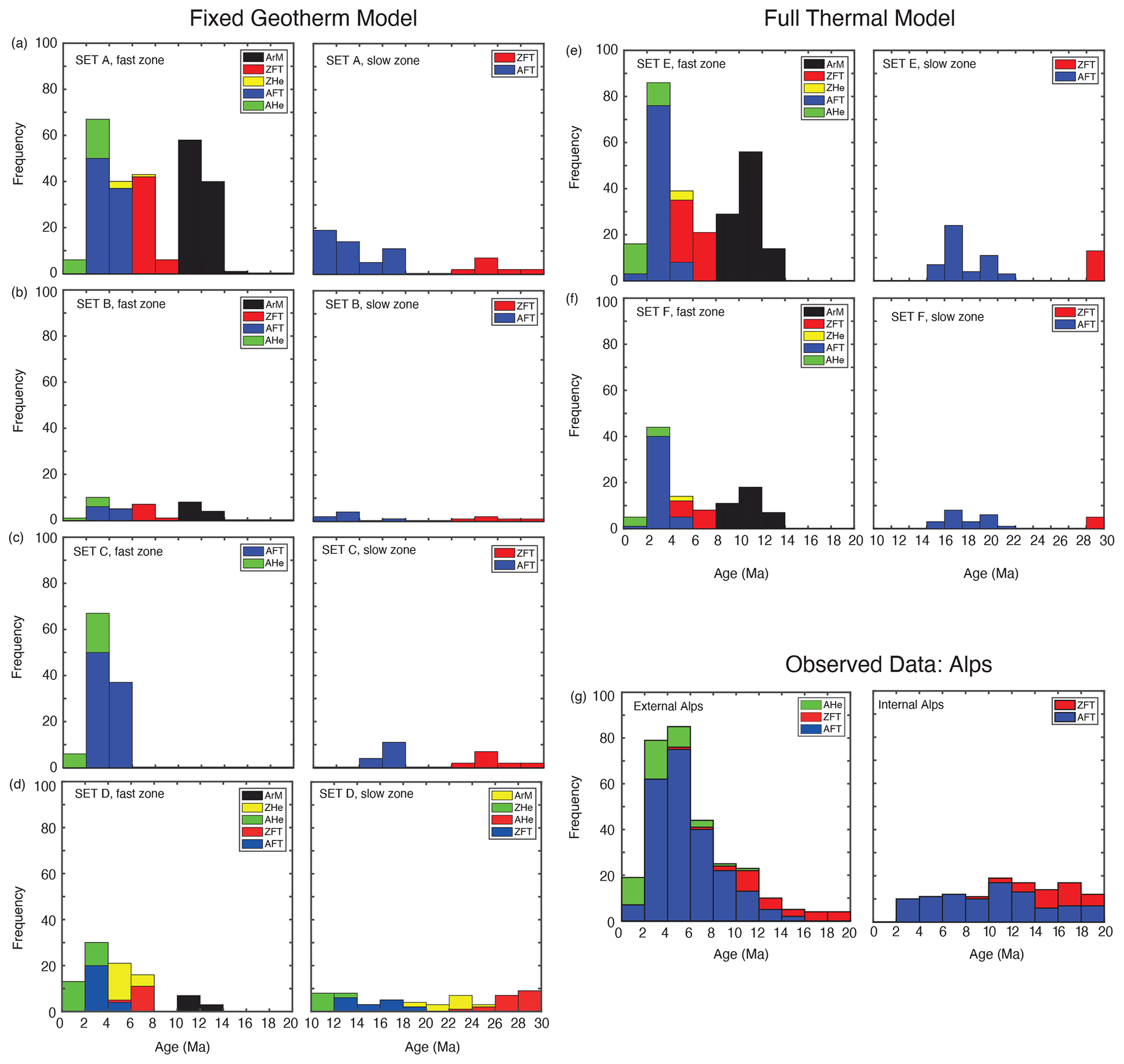
Figure 3Synthetic age data sets for model bias and resolution tests, comprising two zones with differing erosion rates. Colours represent ages from different thermochronometer systems corresponding in closure temperature to green: AHe, blue: AFT, yellow: ZHe, red: ZFT and black: muscovite . Data sets A–D (a–d) were generated using a constant geothermal gradient. Data sets E and F (e, f) were generated using the GLIDE transient thermal model with a flux boundary condition. (g) Observed ages from the Alps to show that the number of data and age ranges are similar to all synthetic data models.
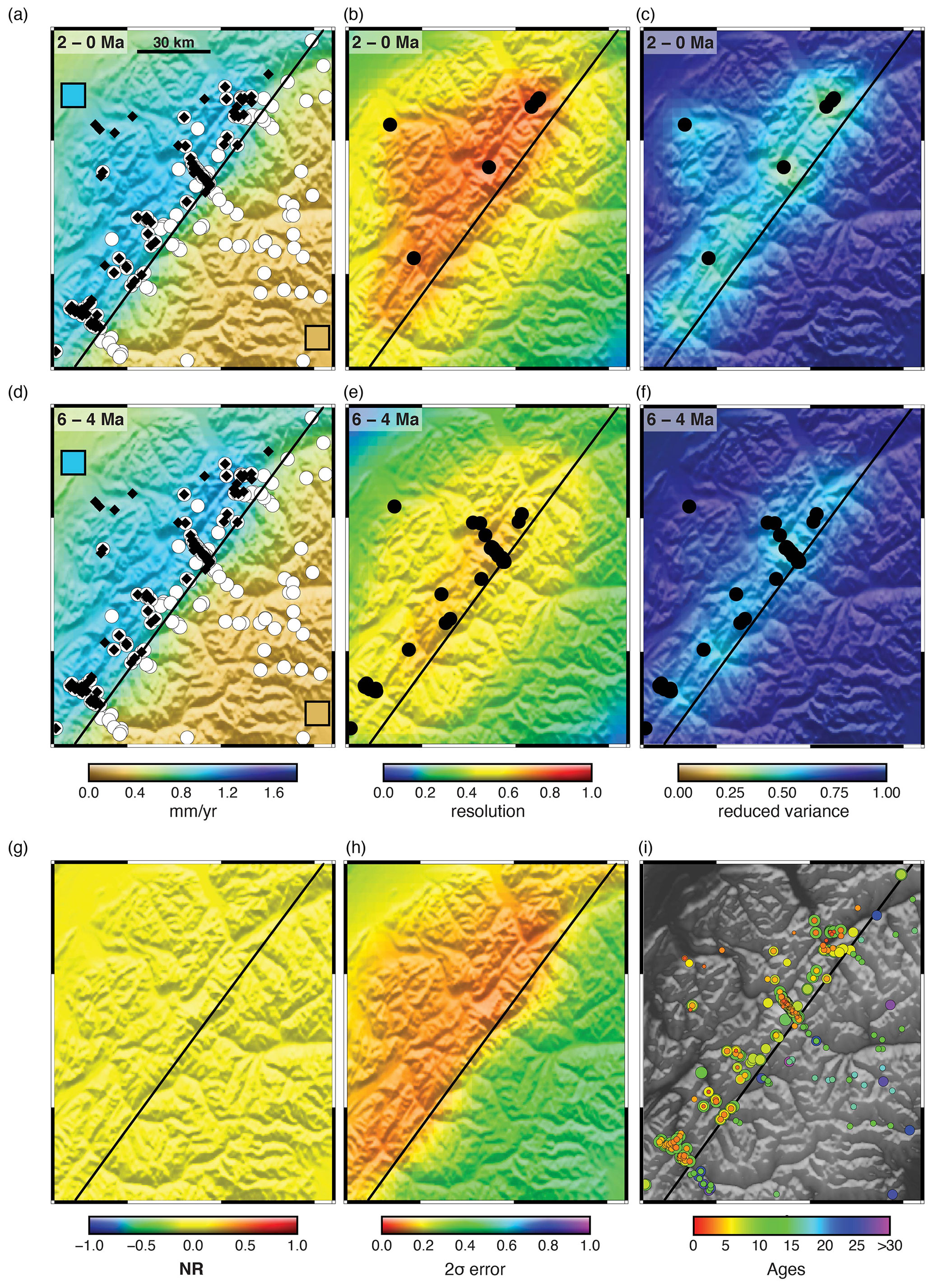
Figure 4Synthetic data test for model errors. The true solution is constant exhumation rate through time, with a high exhumation rate (1 mm yr−1) in the upper-left corner and low exhumation rate (0.25 mm yr−1) in the lower-right corner, identical to the test proposed by Schildgen et al. (2018). Inset boxes in (a) and (d) show the true solution. The thermal model is replaced with a constant geothermal gradient to remove potential errors associated with the geotherm calculation. The correlation length scale (30 km) is given by the black bar in (a). Other parameters are given in Table 1. Synthetic ages are shown in Fig. 3a and (i), where the size of the point corresponds to one of four closure systems, AHe, AFT, ZHe, or ZFT; these are calculated with a constant geothermal gradient in both the forward thermal and inverse models. Data points in (a) and (d) show age locations with ages less than 6 Ma as black diamonds and ages greater than 6 Ma as white circles. Black data points in (b), (c), (e) and (f) show the locations of ages that fall inside the respective time interval. Estimated exhumation rate is shown with the temporal resolution and posterior variance for the time intervals indicated. (g) and (h) show the normalized exhumation rate difference (NR) and its posterior 2σ error. The true solution is recovered very well in the centre region, where data density is high. No spurious acceleration is visible.
To isolate model errors, it is necessary to remove resolution errors. With reference to Eq. (9), resolution errors can be eliminated by one of two ways, either by obtaining a model with R=I or by setting eprior=etrue. Either of these will result in nullifying the entire contribution of the resolution errors. Because we have no data errors (measurement noise), the only remaining errors will be the model errors (Eq. 13).
As a first test (Fig. 4), we attempt to produce a model with R=I. In principle, this requires an infinite number of data, but it will be adequate to simply use a large data set, with ages distributed across the time span of interest (Fig. 3a). The first model results are shown in Fig. 4. These show that the parameters are recovered very well with this data set. The largest errors are in the peripheral regions that have no data, suggesting that these errors are due to inadequate data coverage and so constitute resolution errors. For a perfect test for model errors, we should add more data to these regions. Similarly, some smoothing of the solution is visible across the fault boundary, but this occurs primarily where there are no ages near the boundary on one side or the other of the fault. This smoothing extends less than one correlation length into the adjacent domain and occurs in all time intervals nearly equally; i.e. both the 2–0 and 6–4 Ma time intervals have a small amount of smoothing, so that the net result with respect to inferred acceleration (Fig. 4g) is 0. In fact, there is no trace of spurious acceleration in either the high uplift or low uplift region throughout the model. We calculated the NR (Eq. 14); values are all very close to 0 throughout the domain (Fig. 4g). Interestingly, the variance on the NR is very large in the lower-right half of the domain. This is due to a combination of the lower resolution of this region and the low erosion rate given the dependence of the variance on the erosion rate (Eq. 16). Also interesting is the lack of any acceleration in the low erosion rate domain. There are no ages younger than 6 Ma in this domain, so it does not have ideal resolution, similar to the left-hand side of Fig. 1 with poor resolution for the last 6 Myr. Although we are mainly addressing model errors, this example indirectly addresses the resolution question. According to the spatial correlation hypothesis, the well-resolved, high erosion rates of the upper-left region should be averaged into the late time intervals to the lower-right region. This has not happened in spite of the low resolution. This is an illustration of the importance of the integral nature of thermochronometric ages (Fig. 1). Older ages constrain the integrated erosion rate at their location, so any inappropriate averaging of the high erosion rates to the north-west into the solution in the south-east would result in a misfit to these ages.
For this first test, the smoothing errors that do occur are a function of the spatial correlation, but only weakly. In Fig. 5, we show another version of the model of Fig. 4, using the same data set (Fig. 3a) but with a longer correlation length of 100 km, compared to 30 km in Fig. 4. The results are only slightly different. In fact, the solution in the peripheral regions is improved with the larger correlation length. There is likely more smoothing around the diagonal fault, but the difference is so small that it is not readily visible in Fig. 5. Resolution is higher, but this is because of the definition of the parameters as regional averages, not as local erosion rates. Even with a strong spatial correlation, there is no inappropriate averaging of the high erosion rates into the region of low erosion rate. Therefore, there is no spatial correlation bias, no inappropriate spatial averaging, and no spurious acceleration.
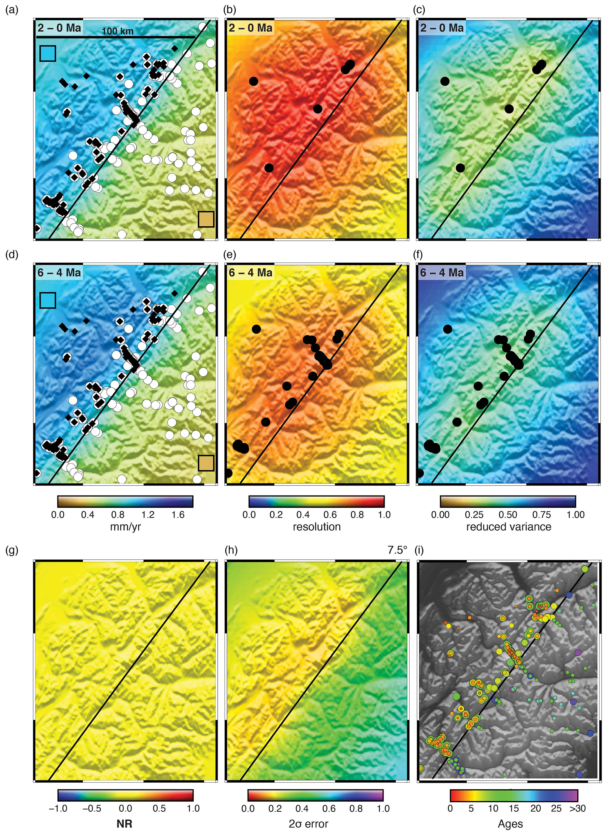
Figure 5Synthetic data test for model error with a correlation length scale of 100 km. The true solution is the constant exhumation rate through time, with a high exhumation rate (1 mm yr−1) in the upper-left corner and a low exhumation rate (0.25 mm yr−1) in the lower-right corner identical to the test proposed by Schildgen et al. (2018). Inset boxes in (a) and (d) show the true solution. The thermal model is replaced with a constant geothermal gradient to remove potential error in the geothermal calculation. The correlation length scale is given by the black bar in (a). Other parameters are given in Table 1. Synthetic ages are shown in (i), where the size of the point corresponds to one of four closure systems, AHe, AFT, ZHe, or ZFT; these are calculated with a forward thermal model identical to the inverse model. See the caption to Fig. 6 for additional details. The correlation length scale is more than 3 times that used in Fig. 4.
As a second test for model error, we eliminate the resolution error by the second method, i.e. setting the prior model equal to the known, true solution. From Eq. (9), this ensures that the resolution errors are 0, and we are left with only model errors. The previous model used a data set with very high density in order to force the resolution matrix to be close to I. In this second test, high resolution is not needed, so we use a sparser data set, shown in Fig. 3c. This is not a trivial test. There is no reason why a model with the correct prior will obtain a posterior solution that is exactly the same. In fact, this is one of the best tests for model bias, because if the test shows errors, these errors indicate a failure in the model, not errors or inadequacies in the data. For example, if the correlation structure is forcing excessive smoothness onto the solution, this will emerge as error in this test. Results are shown in Fig. 6 and are conclusive; there is essentially zero error in this model. Even the peripheral regions with no data, which were not well fit in Fig. 6, show no error. The model shows that there is no model bias associated with the spatial correlation structure. If there are errors in the inversion methodology, they are linked to the resolution of the data and thus to the data distribution. This result establishes that the real issue in these and, likely, most thermochronometric models, is in determining how many data, and in what configuration, are required to constrain a solution and how to recognize and bound resolution errors. This is the subject of the next section.
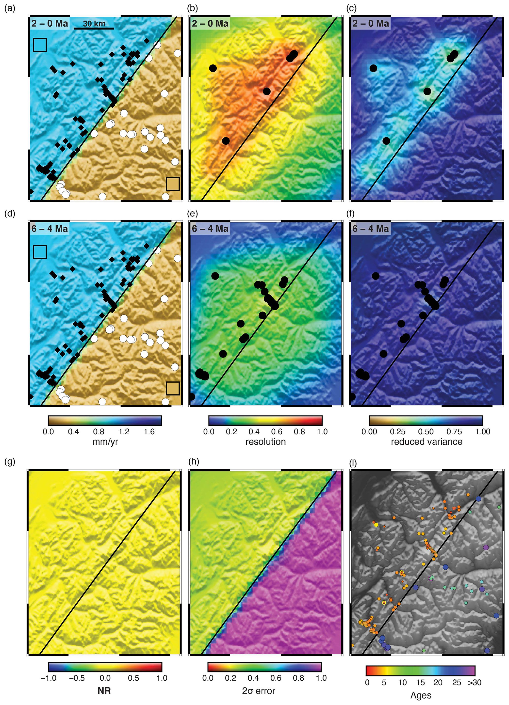
Figure 6Synthetic data inversion test using reduced data density Set C (Fig. 5) and a prior erosion rate of 1.0 mm yr−1 in the north-western corner and 0.25 mm yr−1 in the south-eastern corner. This is equivalent to the true erosion rate used to generate the synthetic ages. Other inversion parameters in Table 1. See the Fig. 4 caption for other formatting details.
4.3 Synthetic data tests for resolution errors
The tests in Sect. 4.3 showed conclusively that there is no model bias in the method of Herman et al. (2013). However, an estimation problem with sparse data such as most thermochronometry problems will be dominated by resolution errors, and model behaviour with sparse data is a much more interesting and important question. In this section, we conduct a suite of tests to determine any potential systematics in resolution errors in the GLIDE inversions.
Resolution errors are easy to calculate but difficult to generalize, because each natural or model data set has a unique distribution in space, elevation and time and therefore unique resolution errors that must be evaluated individually. In the current problem, we are trying to estimate a field quantity (erosion rate) over two spatial dimensions and time, so this is a 3D estimation problem. It is further complicated by the fact that time resolution is controlled entirely by the value of the thermochronometric ages, so we have no experimental control on time resolution, other than by application of different thermochronometers with different closure temperatures. Age variations with elevation increase the time range and are equivalent to having multiple thermochronometer samples with different closure temperatures in this regard, but we will not extensively investigate this aspect of the problem. Given the complexity of possible data characteristics (number, spatial distribution, elevation distribution, closure temperatures, a proper analysis of any specific erosion rate function requires tens to hundreds of experiments. However, by conducting models with a variety of data sets reflecting a range of data sparsity, we can establish the general behaviour of the system and should detect any sort of systematic errors such as a common tendency towards false acceleration.
There is a second purpose to these models. Now that we have established that errors will be errors of resolution, we should assess how well our posterior metrics of resolution and variance characterize this error. Knowing where we have error is in some ways more important than the error itself, as this determines the utility of the analysis in the real world, where we do not know the “correct” answer. We would like to know how well we are able to bound our estimates and where they are unreliable.
The results in Figs. 4 and 5 have already told us something of the importance of resolution. They provide evidence that with good data coverage, we will recover the proper solution with little bias. In fact, the models in Figs. 4 and 5 are not particularly of high data density. The south-eastern corner has no ages under 6 Ma, which implies poor resolution for the 6 to 0 Ma time interval. The high uplift region is well resolved because we generated ages for five independent thermochronometers with different closure kinetics. The synthetic data are well distributed across time to resolve the temperature history over the last 10 Ma (Fig. 3a). There is also an increase in age range for each thermochronometer due to the elevation spread, and this provides additional resolution through the age–elevation relationship. However, prior to the oldest age in the high uplift area, there is no information, so local resolution goes to 0, and there will be a transition from poor to good resolution through time.
We illustrate the importance of age range by conducting inverse model experiments with a second, sparser data set to test the impact on parameter recovery, error, and posterior statistics. Figure 7 shows an inversion experiment using Data Set B (Fig. 3b and Table 1), which has a good age distribution but very few data distributed across space. In spite of the sparsity of data, the solution recovery is very good, with the central region around the data accurately estimated. Peripheral regions are again poorly resolved, but there is no false acceleration emergent from these errors.
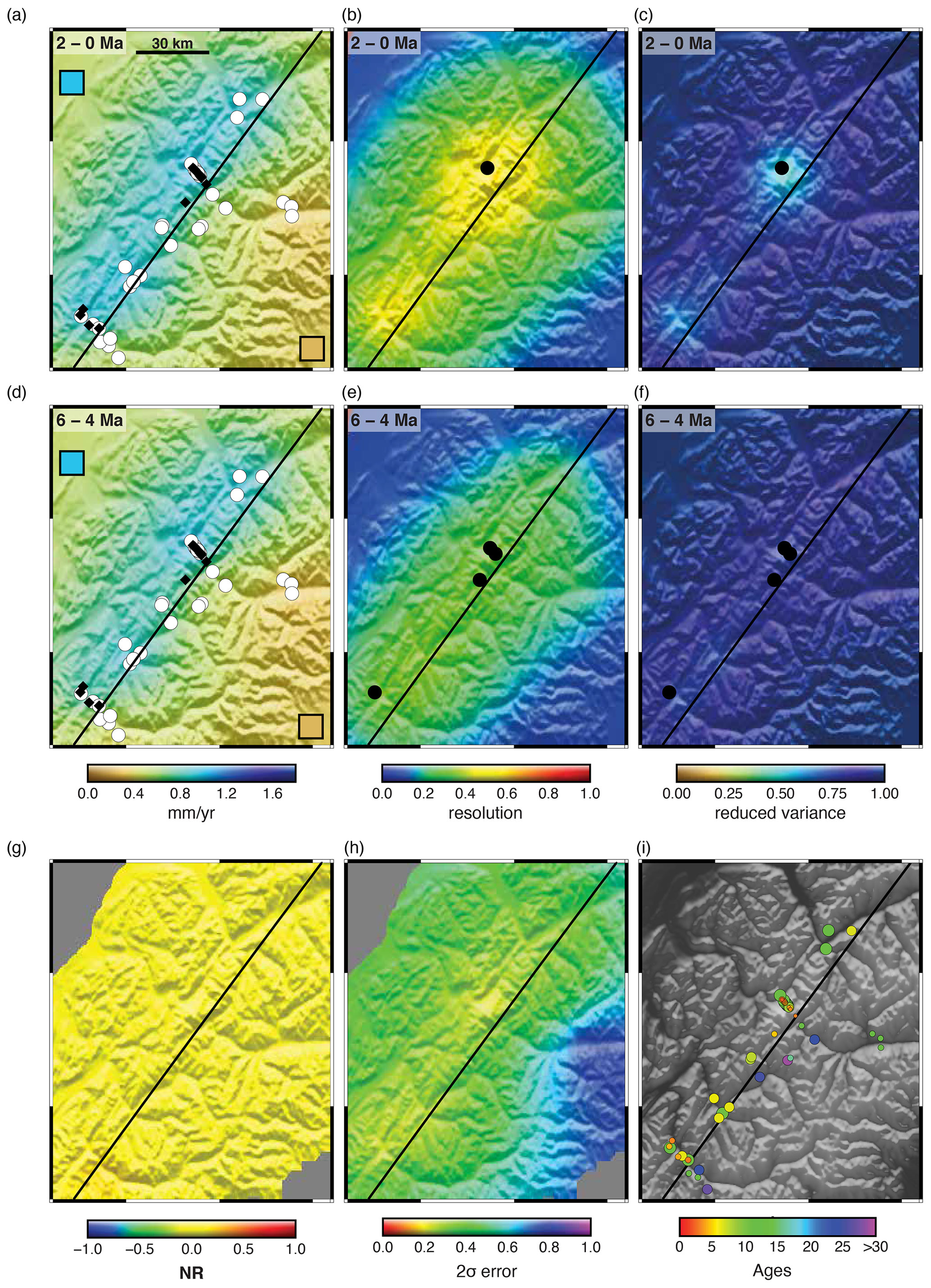
Figure 7Synthetic data inversion test using reduced data density Set B (Fig. 3b). Data have good coverage in time but poor coverage in space. Prior erosion rate is 0.35 mm yr−1. Other inversion parameters in Table 1. See the Fig. 4 caption for other formatting details.
The importance of the posterior statistics becomes apparent with this model. The region of a well-resolved erosion rate in the 2 to 0 Ma time interval is small, and the high values of the resolution statistic surround the data well (Fig. 7b). The maximum resolution is about 0.6, but values of about 0.4 define the accurate solution. The reduced variance plot (Fig. 7c) is more conservative and indicates only a few points where the variance has been reduced to below 0.5. The erosion rate in the 6 to 4 Ma time interval is poorly resolved, with almost the entire model under a value of 0.4.
We constructed another data set (Set C) with better spatial coverage but poor temporal coverage (Fig. 5c) to demonstrate how resolution is dominated by the values of the ages (Fig. 8a). Data Set C has no high-temperature thermochronometers, so all ages in the high uplift zone are less than 6 Ma. Losing the high-temperature systems seriously degrades the quality of the solution. Time intervals older than 6 Ma are almost fully unresolved. The solution accuracy matches the resolution, with a reasonably good solution in the 2 to 0 Ma time interval and a poor solution in the other time intervals. In the slow-uplifting region, the solution is uniformly poorly resolved but not highly inaccurate.
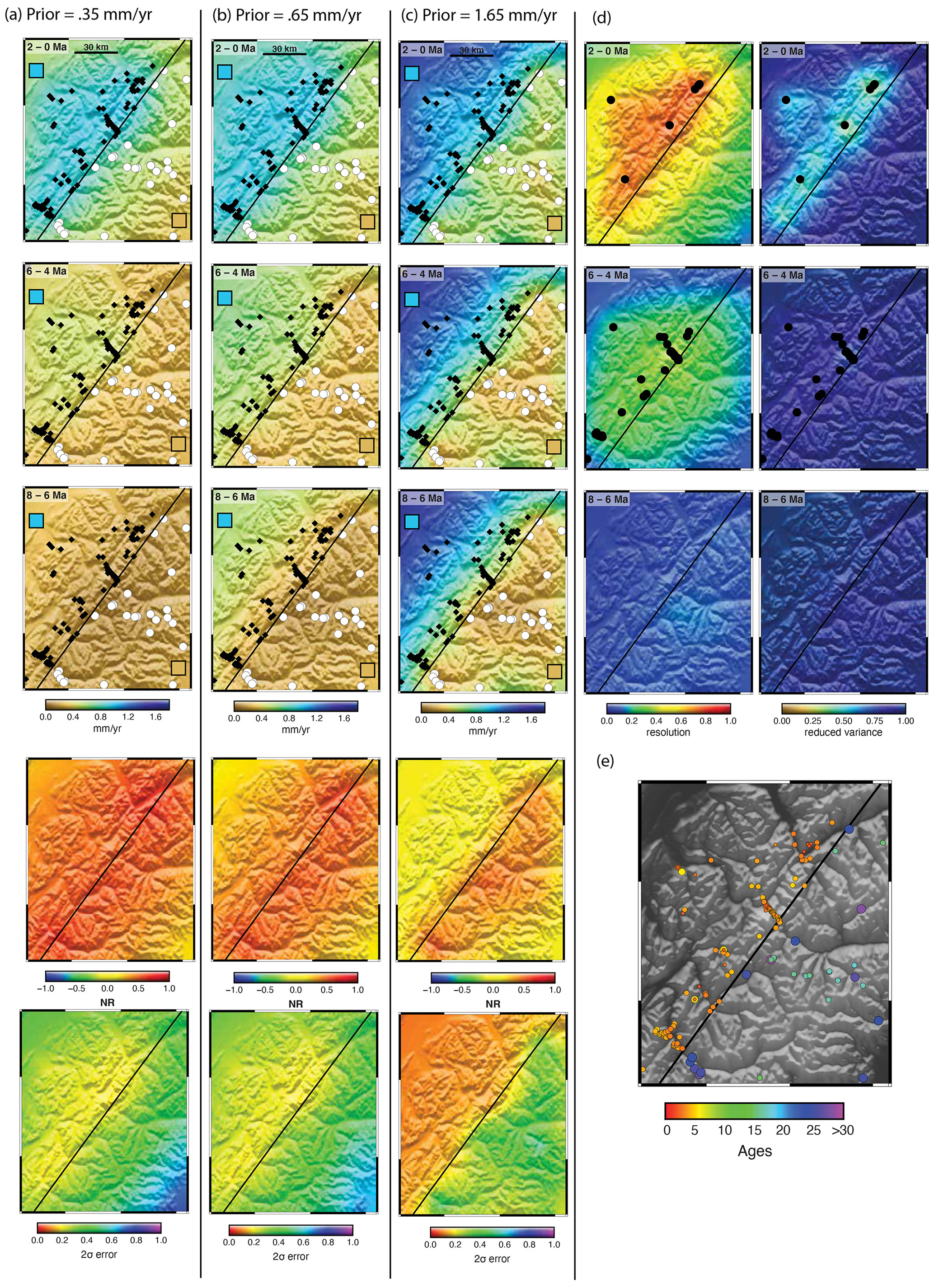
Figure 8Synthetic data inversion test using reduced data density Set C (Fig. 3c). Data have moderately good coverage in space but poor coverage in time. Prior erosion rate is (a) 0.35 mm yr−1, (b) 0.65 mm yr−1, and (c) 1.65 mm yr−1. (d) Temporal resolution and reduced variance applicable to all three models. (e) Age data. Other inversion parameters in Table 1. See the Fig. 4 caption for other formatting details.
The poor resolution of this model is useful for demonstrating another important characteristic of Bayesian models such as GLIDE. As shown in Eq. (12), as the resolution goes to 0, so does the inverse operator, and the solution will revert to the prior solution. This is what we observe in Fig. 8a, where the prior model has a uniform value of 0.35 mm yr−1. Everywhere in the model where the resolution is low, the erosion rate reverts to a value of 0.35 mm yr−1. This is particularly apparent in the earlier time intervals where there are no ages controlling the rate; the erosion rate here has nearly uniformly taken the prior value. The corresponding resolution is near 0 and the variance is not reduced below its prior value, so it is clear that this is not a resolved parameter. We confirm this finding by running the same inversion, with different values of the prior erosion rate. Figure 8b and c show models with Data Set C and all other parameters as in Fig. 8a, except that the prior erosion rate is set to 0.65 and 1.65 mm yr−1, respectively. The differences between these models demonstrate the influence of the prior on the estimate. The regions of the model with low resolution are sensitive to the prior, but the bias depends on why the resolution is low. If there are no older ages constraining a time interval, as in Fig. 1a, right column, the solution takes a value at or near the prior. If, however, resolution is low but there are still older ages constraining the average erosion rate, as in Fig. 1a, left column, the solution takes an average erosion rate consistent with the older ages. If there is a dependence on the prior model, it is weak. Regions with good resolution, for example the central part of the high uplift region from 2 to 0 Ma, have little to no dependence on the prior. The solution in these areas is robust in that time interval. However, in the high uplift region the earlier time intervals are poorly resolved; even the 6 to 4 Ma interval has no point with resolution higher than 0.4, and at this level of resolution, it still shows sensitivity to the prior model. The low erosion rate region is less sensitive to the prior because the ages, which are all over 10 Ma, constrain the average erosion rate over these time intervals. However, individual time intervals are not resolved. Given the sensitivity to the prior and the low values of resolution and variance, the low-erosion rate region in these models should be regarded as unresolved, whereas parts of the high erosion rate region could be regarded as marginally acceptable.
The model of Fig. 6 can be included with the models of Fig. 8 to define a suite of four examples where the only inversion parameter that has changed is the prior value of the erosion rate. Note that the resolution and posterior variance do not change between these four models, because these metrics depend on the data and the prior variances but not the prior erosion rate. The same is not true for the variance of the NR because of its dependence on the value of the erosion rates. Surveying the solutions of all four of these models, we see that the range of outcomes for the NR is very wide, from no acceleration (Fig. 8) to acceleration everywhere (Fig. 8a and b) to neutral or deceleration in the high uplift zone with acceleration in the low uplift zone (Fig. 8c). This range of behaviour is the result of combining the poorly resolved 6 to 4 Ma interval with the well-resolved 2 to 0 Ma time interval. The former depends on the prior model and the latter is reasonably robust and accurate. Although interpretation of the NR with this variability would be problematic, this problem is largely avoidable by noting the error in the NR. The variance in the NR is almost always large, indicating that the values entering the ratio have large uncertainty, and so the NR itself is highly uncertain. The low uplift rate region never has a standard deviation under 0.5, indicating that the NR is never resolved in this region. The high uplift rate region has a lower standard deviation on the NR and could be considered to be on the edge of resolved, and in fact it is these regions that appear resolved by the other metrics as well. The solution is moderately accurate here, although there are still dependencies on the prior, so we would interpret this solution as marginally reliable.
As a final test of resolution errors, we directly test the influence of the ages from the low uplift rate region on the high uplift rate region by removing all ages from the low uplift rate region and inverting the remaining ages. This should remove any spatial correlation bias, leaving only resolution bias. For this test, we constructed an additional synthetic data set that had a more uniform spatial distribution to illustrate spatial smoothing effects without a superimposed data density effect (Set D) (Fig. 3d). Figure 9 shows three models using this data set. There are two models in the leftmost columns using the full Data Set D but different values of the prior erosion rate of 0.35 and 1.0 mm yr−1. Resolution and reduced variance do not depend on the prior erosion rate and so are applicable to both models. On the right is a model with all data removed from the low uplift rate region. This model has a prior erosion rate of 0.35 mm yr−1. We do not show the corresponding model with the half data set and a prior of 1.0 mm yr−1 because it returns exactly and uniformly the correct erosion rate of 1.0 mm yr−1. To provide a more complete temporal view, we show seven time intervals reaching 14 Ma, where the first ages appear in the high uplift zone. The full data model evolves much as the other models above. The fast uplift rate region has no resolution in the early history because there are few or no ages that sample this part of space–time parameter space. Solutions depend strongly on the prior value and resolution and variance reduction characteristics are low. As time progresses and ages begin to appear in the fast-uplift area (12 to 6 Ma), the resolution increases and the accuracy of the inferred erosion rate increases. By 6 Ma, there are sufficient ages on each side of the fault, so that the erosion rate is correctly inferred. There is smoothing across the fault, but this error diminishes as resolution increases at younger times.
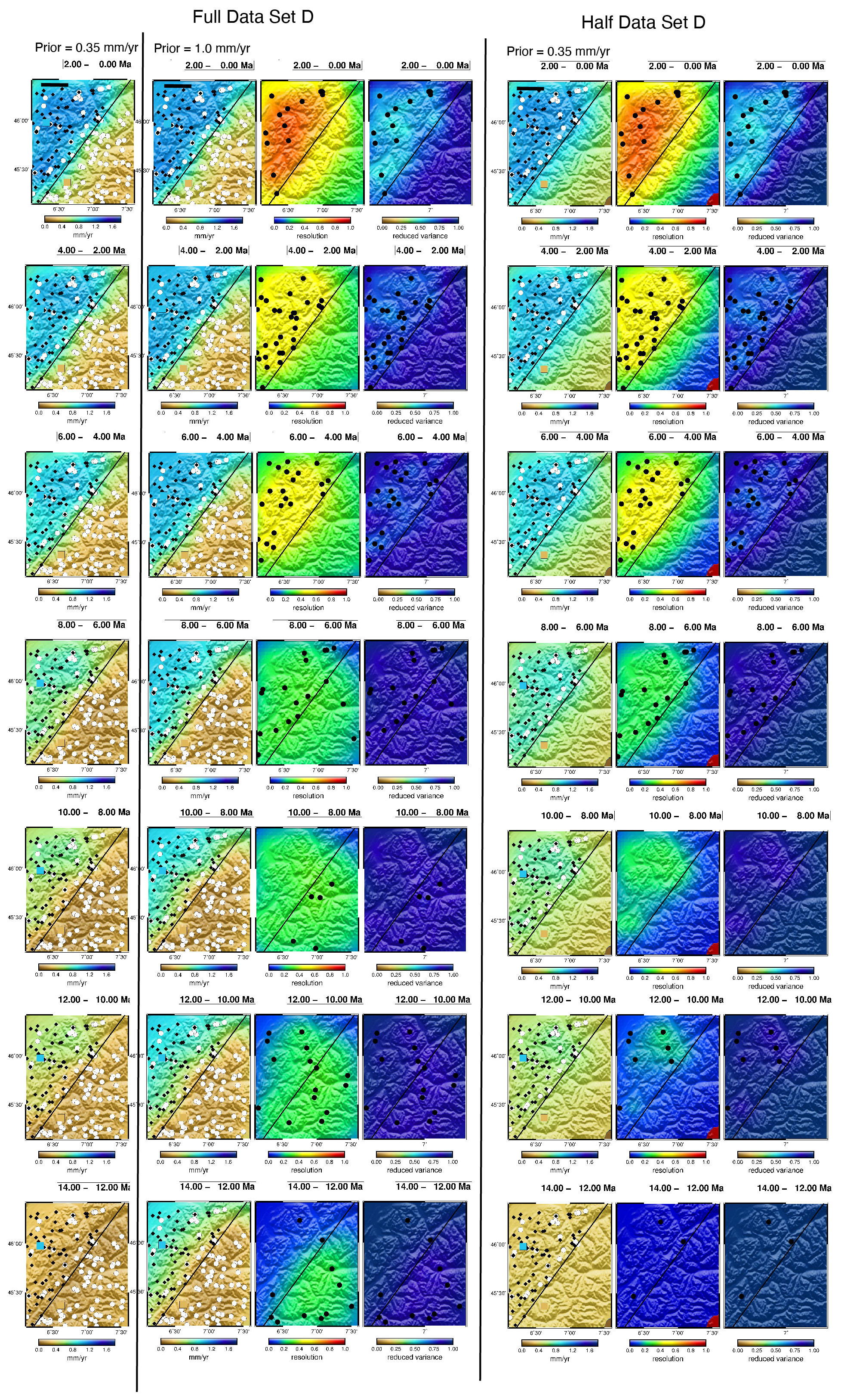
Figure 9Synthetic data inversion test using reduced data density Set D (Fig. 3d). Prior erosion rate is 0.35 and 1.0 mm yr−1. In the right column, all age data from the low uplift region (south-east) are removed. Other inversion parameters in Table 1. See the Fig. 4 caption for other formatting details. The similarity in the NW region of the two models shows that there was no spatial averaging of older ages into the high uplift region.
The right three columns of Fig. 9 show the estimated erosion rates for inversion of only the data in the north-western (high erosion rate) region. The result is almost identical to the model with the full data set and low prior (compare columns 1 and 5). Both solutions still have large errors in the early time steps where there are few data constraints, but their similarity indicates that these are resolution errors, not spatial averaging errors. There are differences in predicted erosion rates, but these are limited to the immediate proximity of the fault (less than one correlation length). As in other models of our paper, the spatial correlation errors are largest where there are no data near the fault, indicating that the spatial correlation is not averaging age data so much as interpolating empty space between the data. Spatial smoothing is also visible in the high prior, full data set model, again limited to the immediate vicinity of the fault. There are much larger errors in the low erosion rate region, but these are resolution errors in the half data set model introduced by the removal of all data from this region.
4.4 Trade-offs and age misfit
Estimated erosion rates in the GLIDE model represent a balance between three factors: (1) fit to the age data, (2) consistency with the prior probability model, and (3) averaging with nearby data in space. A parameter estimate is a weighted average of these three types of data where the weights are a function of the correlation length parameter, the data variance (assumed errors in the ages) and the prior erosion rate variance. In particular, the averaging between the prior model and the data is controlled by the ratio of the data variance to the parameter variance, which serves as a regularization or damping parameter for the problem. We saw above that in the absence of data constraints, the parameters revert to the prior model. Similarly, if the data number or quality goes to infinity, the ratio between the data variance and the prior variance is small and the solution will be required to fit the data. This suggests an additional test that can be conducted to estimate the relative importance of spatial smoothing or low-resolution reversion to the prior model. Data residuals, that is, the difference between predicted ages and observed ages, provide a metric for relative weighting between data fit and the other two factors, spatial smoothing and fit to the prior.
We demonstrate this characteristic with the age residuals from the full data model of Fig. 9; residuals are shown in Fig. 10a. As we discussed with reference to Fig. 2, it is not possible to fit different ages with a common temperature history if they have the same elevation above the closure isotherm, so where spatial averaging is occurring, it appears as a difference between predicted and observed ages. This is also true for errors resulting from excessive weight on the prior. Where the prior model is pulling the parameter estimate towards a false value, the age will no longer be fit. Figure 10a shows two groups of large residuals in age. These correspond to the youngest ages in the low erosion rate zone and the oldest ages in the high erosion rate zone. The residuals are opposite in sign. The misfit of the low erosion rate ages is a spatial correlation effect. The predicted ages are too young because of smoothing of the high erosion rates into the low erosion rate zone during the late time steps when resolution to the south-east is low. The large residuals all come from data close to the boundary fault, where one can see the erosion rate errors as edge smoothing in Fig. 9; ages in this region are misfit. The residuals in the high uplift region are different. They include the spatial correlation errors but also a bias to the prior given that the prior erosion rate is low. We can try to separate these by changing the prior model. However, rather than changing the prior erosion rate, which has a large effect on the estimated parameters, we ran a new model where we increased the prior variance on the erosion rate. By increasing the variance, the influence of the prior is reduced and the relative weight of the age data is increased. The residuals for this model are shown in Fig. 10b. The misfit to the ages in the low erosion rate region is unchanged, but the residuals in the high uplift region are now close to 0. This indicates that we have obtained a more accurate solution with decreased weight on the prior, identifying that the errors in the high erosion rate region were dominated by resolution errors and bias to the prior. The prior variance in all the models so far has been small (standard deviation of 0.1), which implies a strong influence of the prior on low-resolution time steps.
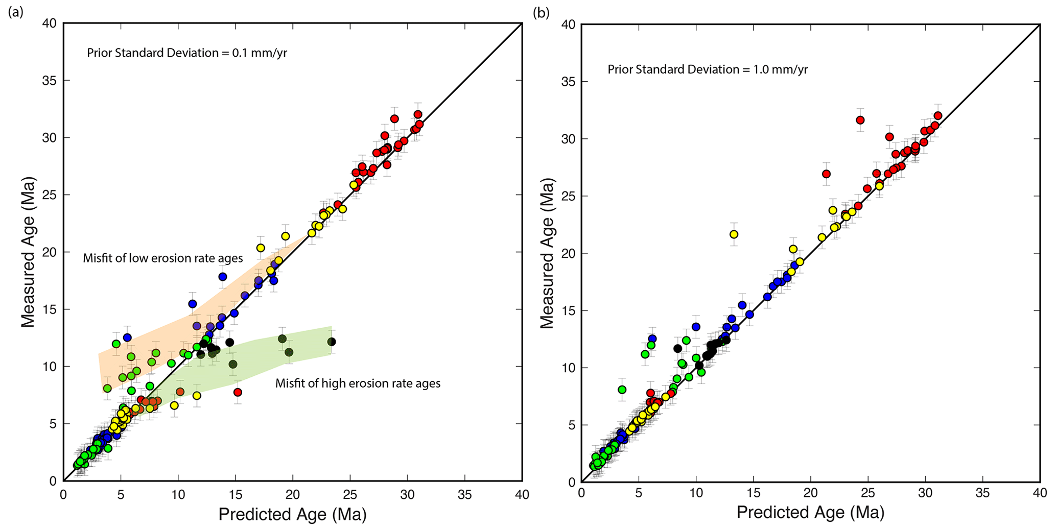
Figure 10(a) Data misfit for the left model in Fig. 9. Prior erosion rate is 0.35 mm yr−1; prior standard deviation of the erosion rate is 0.1 mm yr−1. (b) Inverse model of the same data but with a prior standard deviation of the erosion rate of 1.0 mm yr−1. Reduced residuals in (b) show that the errors were due to bias in the prior, not spatial averaging.
The large residuals reflect the transition from poorly resolved time steps to well-resolved time steps. The model of Fig. 9 as well as several of the models using Data Set A have inaccurate parameter recovery for the high uplift rate zone in the 6 to 10 Ma range. This is surprising given that the model included a relatively large number of ages across this interval. An explanation is provided by the data residual analysis. The ages that are misfit in Fig. 10a are in this 6 to 10 Ma range. It is apparent that the estimated solution has a strong tendency to stay at the prior value rather than fit these ages. During the early history, there are no ages to constrain the high uplift rates, so the solution stays at the low value of the prior. During progressively younger time steps, the high uplift zone ages begin to appear and pull the solution towards the correct, high value. However, during this transition (approx. 10–6 Ma in this model) the number of ages is insufficient to counter the weight of the prior. Only as more young ages come into the problem (approx. 8–4 Ma) can the ages pull the solution fully from the prior to the correct value. The number of ages required to obtain an accurate solution is large compared to most natural examples, but this is a consequence of the extreme conditions of this synthetic model. In the high uplift zone, the true erosion rate is 7 SD (standard deviations) away from the prior erosion rate for the full 30 Ma of the model run. These conditions place a strong demand on the data in order to balance the effect of the prior model which is far from the true solution. Even the tens of data present in Data Set A or D over the 6 to 10 Ma window were not sufficient. By increasing the prior variance (Fig. 10b), we have reduced the weight of the prior; the ages are again fit, and the erosion rates are estimated accurately. Most natural cases, without such an extreme erosion rate history, would require fewer data to counterweight the prior and obtain the correct solution. Normally in a model study with such a large variation in erosion rates, we would have increased the prior variance so that fewer data were needed to achieve an accurate solution, but we thought it important to keep the inversion conditions of Herman et al. (2013), even for these extreme models. As is always the case, an artificial model cannot be directly translated into a prediction of behaviour in a natural case. What can be taken from these models is that there will always be a transition between a poorly resolved time interval, where an estimate is influenced by the prior model and a well-resolved interval where age data are sufficient to constrain the solution to the correct solution. Where that transition is depends on the number and precision of data and the relationship between the true solution and the assumed prior model and must be estimated on a case-by-case basis from characteristics such as resolution metrics and data residuals.
An important caveat to all the models in this section is that the analysis applies only to the case where data are accurate and consistent with the forward model. In nature, this will not be the case, as there will always be differences in cooling processes or diffusion kinetics that are not accounted for in the model. In this case, estimated parameters may be pulled in directions other than to the prior or to the true solution. For this reason, some regularization of the model and misfit to the data is always desirable.
4.5 Synthetic data models for an erosion rate gradient
The models thus far have all considered the case of a sharp discontinuity in erosion rate. The other common case, hypothesized to be important in creating false inferences of erosion rate increase, is a gradient in erosion rate and thus age. We reconstructed a simple example of a gradient model by generating ages using a constant gradient of erosion rate from 0.1 to 1.0 mm yr−1 across a 90 km domain (Fig. 11b). We generated ages using four thermochronometers but no variations in elevation. Data were generated on a regular grid to avoid non-generalizable effects arising from randomized positions and elevations. This model is effectively 1D, but we portray results in map form to be consistent with the other models. A fixed geotherm was used to avoid model errors. Results are shown in Fig. 11, with additional models in Appendix A. The true solution is recovered nearly perfectly over the last 6 Ma. As with the other models, as resolution deteriorates back in time, the solution reverts to the prior parameters (Fig. A2). We constructed a suite of models using subsets of the data and changing the prior model and correlation length (Figs. A3–A6). In all cases, in the absence of data constraints, the solution reverts to the prior, but there is no evidence for spatial correlation errors. Larger correlation lengths actually improve the model predictions, which is not surprising given that a constant gradient in a function corresponds to perfect spatial correlation. Interesting in these models is that it is the older, zircon ages that provide the best constraints on the erosion rate history. The absence of young ages does not lead to large errors in the case where the exhumation rate is steady. Provided that there are older ages to constrain the long-term average exhumation rate, there is no tendency to a false acceleration (Fig. A4).
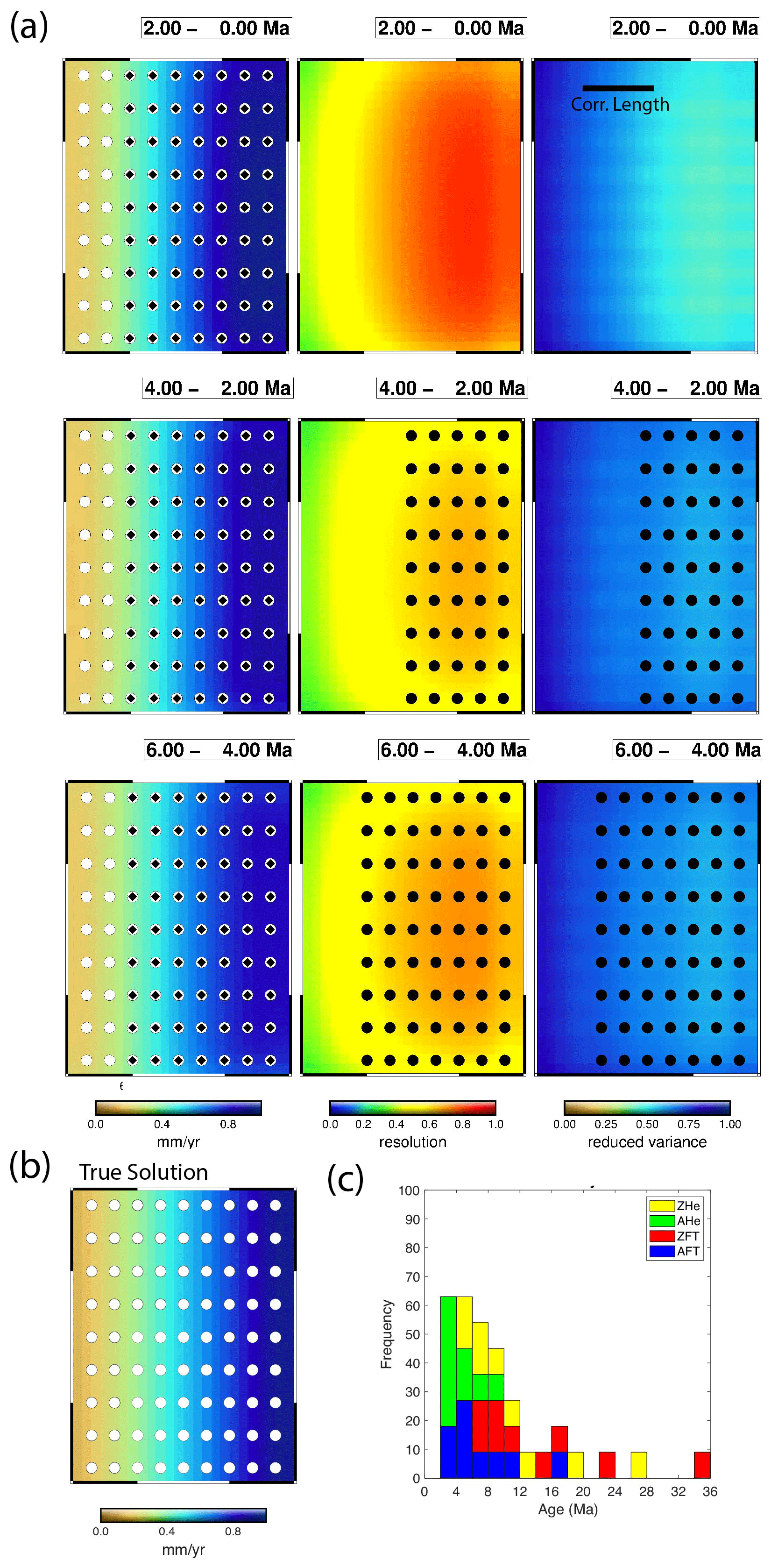
Figure 11Synthetic data model for a gradient in erosion rate varying from 0.1 mm yr−1 on the left edge to 1.0 mm yr−1 on the right edge. True solution and data locations are shown in (b). Ages are shown in (c). All four thermochronometers are given at each data location. There are no variations in elevation. Inverse solutions for the last three time intervals shown in (a). Other models including for subsets of data shown in Appendix A.
These models are consistent in their result. There is no visible effect of spatial averaging and no false inference of an increase in erosion rate due to spatial averaging along the age gradient. There are resolution errors for early time intervals that are poorly sampled by ages, where the solutions revert to the prior model, but for young time steps that are poorly resolved but have older, high closure-temperature ages, the solution remains accurate because it is constrained by the older ages that provide an integral constraint on the erosion rate. This result reflects the two principles we expressed above. First, correlation is not equivalence, and a linear variation in erosion rate implies perfect correlation of erosion rates without requiring that they be equal or averaged. Second, erosion rates cannot vary to fit neighbouring ages without a large misfit to local ages. For a steady erosion rate with a spatial gradient, any temporal variations in erosion rate that do not satisfy the integral constraint will result in age misfit, so there is no statistical advantage in creating an erosion rate history with a false increase in rate.
4.6 Synthetic data models for errors in the thermal model
All models above use a thermal model that has been simplified from the normal, transient model incorporated into GLIDE. This was done to remove the coupling between the thermal model and erosion rates that can lead to complex error propagation. At low erosion rates, heat advection is small and the effect on the geotherm is small, but the test model we are using includes a region with an erosion rate of 1 mm yr−1 for 36 Myr, so the advective component of the heat flux is large and the geothermal gradient increases by a factor of nearly 4 (Fig. 3). This is extreme compared to the real world, where such large erosion rates are rarely sustained for long, but as a test case, extreme conditions are acceptable. However, unless the high uplift area has thermochronometers with very high closure temperatures, ages are unlikely to exceed 15 Ma (Fig. 3), which leaves the first 20 Ma of the thermal history unconstrained. In the absence of data constraints, the erosion rate reverts to the prior value. For any synthetic test with a low prior erosion rate, the geothermal gradient will be badly in error, leading to errors in the erosion rate. Geotherm errors are primarily a non-linear, and often negative, multiplier to errors in the erosion rate. For example, if erosion rates early in a thermal history are too low because of a low prior, the geothermal gradient will be too low and the late history erosion rates will be too high to compensate and fit the data ages.
To demonstrate some of these effects, we generated two synthetic data sets using the full transient model internal to GLIDE (Sets E and F, Fig. 3e and f). Set E has good temporal coverage in the high uplift region but poor coverage of the low uplift region. Set F has poor spatial coverage for the entire domain. To demonstrate that the thermal model does not introduce any model errors, we first invert Data Set E with the prior model set equal to the true solution. As above, and following Eq. (12), this eliminates the resolution errors, leaving only model error; results are shown in Fig. A6. As in all other models with the prior solution set equal to the true model, the true solution is recovered nearly perfectly, so there are no model errors or method bias. By setting the prior model to the true model, the thermal model is now correct, meaning that it is equivalent to the model used to generate the ages, so there are no model errors arising from spatial correlation, data smoothing, the geotherm calculation or other sources related to the model. Any errors in subsequent models are due to data inadequacy, i.e. resolution, and resolution errors amplified by subsequent errors in the thermal model.
As a second experiment, we inverted Data Set E using a prior erosion rate of 0.35 mm yr−1 (Fig. 12). The data distribution and number in this model are close to those of Data Set A, so we expect the resolution errors to be small (see Fig. 6), but errors are considerably larger. The difference is the amplification due to model error in the geotherm. Errors are largest on the high uplift side of the fault but are present on both sides. Estimated erosion rates are significantly larger than the true values. This is a consequence of an estimated geothermal gradient that is too low. Although the errors are large, they produce a false deceleration, not an acceleration. This indicates that not only is the average gradient in the geotherm incorrect, but also that the curvature is incorrect. Because of the error in the geothermal gradient and curvature, a low prior (as used in Herman et al., 2013) is likely to produce a false deceleration in regions of sustained high uplift, although we would not over-generalize this result.
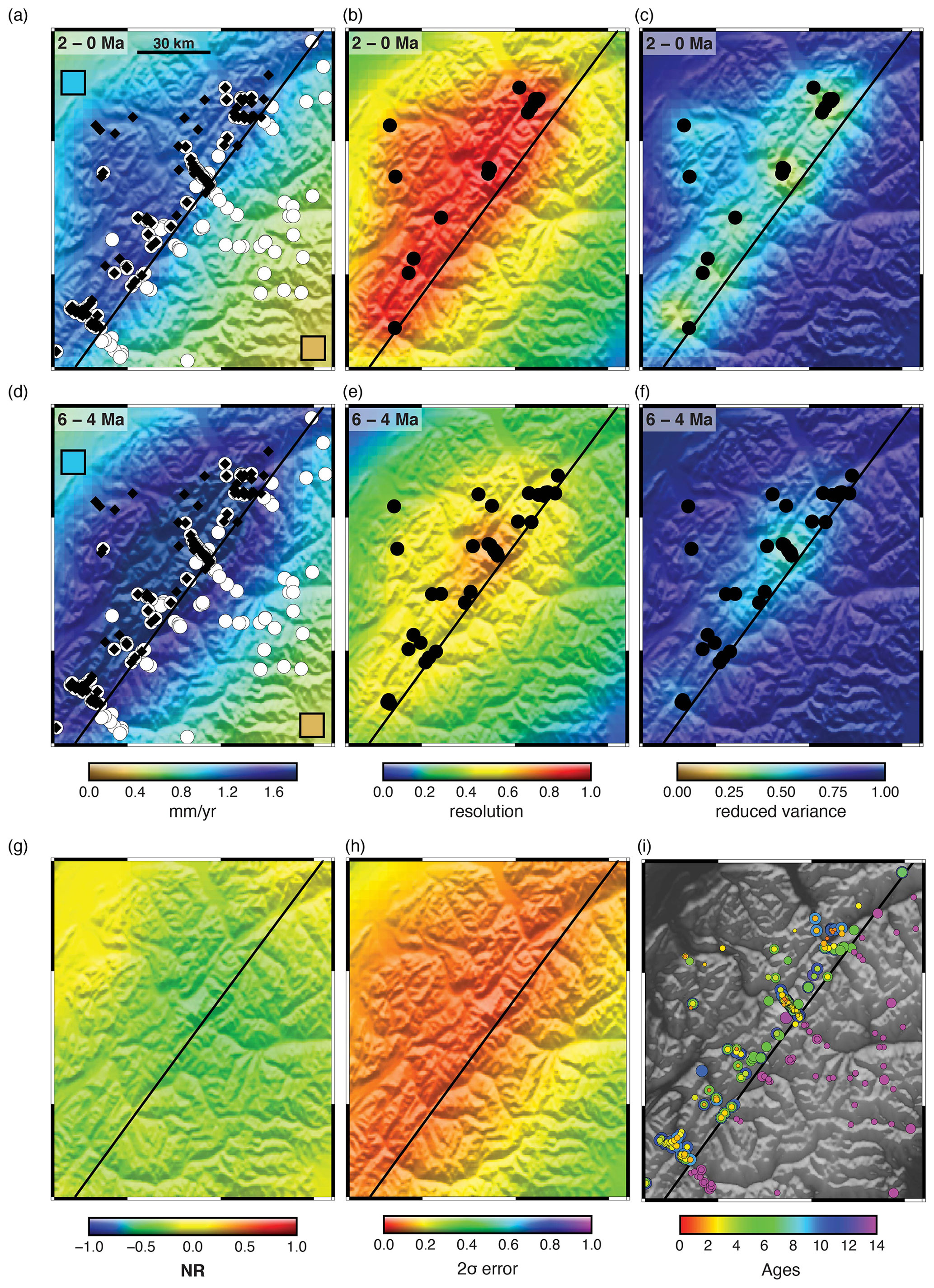
Figure 12Synthetic data inversion test using synthetic Data Set E calculated using the full, transient thermal model internal to GLIDE (Fig. 3). The prior erosion rate is 0.35 mm yr−1. Other inversion parameters in Table 1. See the Fig. 4 caption for other formatting details.
As an additional test of mixing resolution errors with model errors, we decimated the test data set to make a sparse data set, although we kept the temporal range appropriate for the time range of interest (Fig. 3f). Inverting with the low prior value (Fig. 13) gave a result similar to Fig. 12, although the spatial domain was much noisier, with highs and lows depending on the data locations and values. Where Fig. 12 shows a uniform deceleration, Fig. 13 shows a mix of acceleration and steady regions, with the best resolution indicated for the steady regions. Resolution metrics show that the 6 to 4 Ma time interval is only marginally resolved, whereas the 2 to 0 Ma time interval is well resolved.
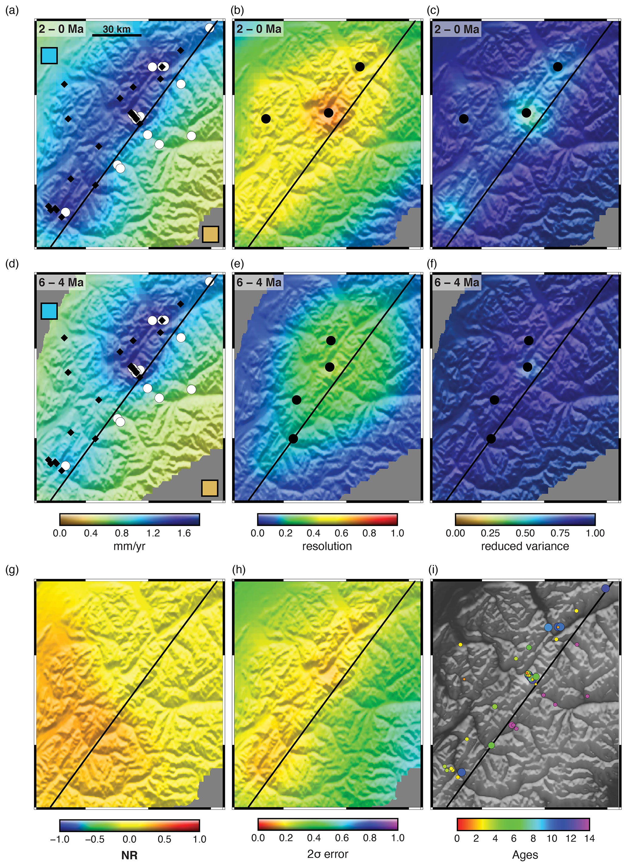
Figure 13Synthetic data inversion test using synthetic Data Set F calculated using the full, transient thermal model internal to GLIDE but sparse data (Fig. 3). The prior erosion rate is 0.35 mm yr−1. Other inversion parameters in Table 1. See the Fig. 4 caption for other formatting details.
Thermal model errors are difficult to identify in the posterior statistics. A systematic geotherm error does not appear in either resolution or posterior variance metrics, and regions that these metrics indicate as well resolved can have very large errors. This is different from the resolution errors, which were well characterized. The best solution to this problem in natural problems is to minimize model errors by calibrating the final geothermal gradient against modern heat flow measurements (Willett and Brandon, 2013). In some cases, pressure–temperature–time constraints from metamorphic assemblages might serve the same purpose, but the time component is necessary if the geotherm is transient. In the synthetic data models of this paper, we could have calibrated each model to the final gradient used to generate the ages and we would have obtained much more accurate models, but following the methodological principle of isolating error and variables, we chose rather to hold the initial condition constant for all models. Again, we would like to emphasize the point that the synthetic data models presented here are not intended to simulate actual applications, nor do they represent the way in which the inverse model would be applied to a natural example; they are numerical experiments intended to give insight into the performance of the methodology and sources of errors.
In this section, we turn our attention from error analysis to discuss spatial variability in thermochronometer ages in tectonic settings as characterized by both thermokinematic models and natural data studies. The synthetic data experiments (Sect. 4) showed that spatial gradients, or spatial discontinuities, introduce no significant errors, systematic or otherwise, to the GLIDE model inversion, provided data coverage is adequate. We also showed that data adequacy is defined more by the temporal coverage provided by multiple thermochronometers and the elevation distribution rather than the spatial coverage of samples, so it is somewhat of a misdirection to stress spatial variability. Nonetheless, having extensive regions of spatially uniform exhumation rates increases the probability that one can obtain good age–elevation profiles or can combine age data from independent thermochronometers that are not perfectly co-located and still achieve good resolution. The resolving capability of data is determined by the complexity of the erosion rate field being sampled, so resolution should be evaluated in the context of tectonic variability. The following sections discuss spatial variability and age patterns from the modelling literature, make an evaluation of age variability and resolution in a set of natural examples, taken from the original study of Herman et al. (2013), and, finally, provide a discussion of how one can, or cannot, differentiate between tectonic and climatic variability impacts on erosion rate.
5.1 Tectonic settings and age gradients
There has been considerable work done with thermokinematic and thermodynamic models to provide prediction of the relationship between erosion rate and thermochronometric ages (e.g. Mancktelow and Grasemann, 1997; Stüwe and Hintermüller, 2000; Ehlers and Farley, 2003; Braun, 2002b; Braun et al., 2012; Nettesheim et al., 2018; Koptev et al., 2019). Many of these studies have demonstrated that, even in complex tectonic settings, there are broad regions characterized by constant rates of exhumation and thus constant thermochronometric age. It should be noted that when we speak of gradients in age in kinematic models, we refer only to gradients in cooling age, where the cooling is related to the last phase of orogeny and exhumation. In any tectonic setting, there is a contrast between active areas exhibiting young cooling ages and the surrounding regions unaffected or weakly affected by current tectonics (e.g. the pre-orogenic ages of Willett and Brandon, 2002). Pre-orogenic ages are typically tens if not hundreds of millions of years old, and such ages are either removed from the analysis if they are older than the model runtime or, if left in, have minimal effect, given that an age whose exhumation spans multiple time intervals, devoid of other ages, has little influence on the young history, e.g. Fig. 11. In addition, the fundamental concepts of the thermal model, including the definition of a closure temperature, are predicated on monotonic cooling, so multiple heating episodes cannot be resolved.
Some examples of tectonic settings and the predicted distribution of cooling ages are illustrated in Fig. 14, taken directly from the literature cited in the caption. In extensional settings (Fig. 14a), most exhumation occurs by erosion on uplifted footwall blocks of normal faults. Footwalls are often tilted or flexed in response to unloading during fault slip, so one would expect a gradient in exhumation rate with the highest rates found near the fault. One of the most studied normal-fault systems is the Wasatch Fault in Utah, which has extensive thermochronometry data, including both AFT and AHe data (Armstrong et al., 2003) and a complete suite of thermokinematic models (Ehlers et al., 2001, 2003). These studies demonstrated footwall tilt and a gradient of exhumation rate but also showed that at high rates of exhumation, the gradients in age were reduced to the point that they could barely be resolved. This was supported by the observations. Within 20 km of the fault, AFT ages were constant within error (Armstrong et al., 2003). AHe ages showed a small gradient, which, after correction for elevation effects, resulted in a difference of about 3 Ma over a 20 km transect. The low spatial gradients are a consequence of the high rate of exhumation, which compresses the age–exhumation rate relationship. The Wasatch studies are most notable for their extensive sampling with two thermochronometers (AFT and AHe), and it is the age difference between AFT and AHe that resolves a temporal change in erosion rate (Ehlers et al., 2003). Ehlers et al. (2003) found a small decrease in exhumation rate in the last 5 Ma, whereas Herman et al. (2013) found a small increase; this difference is due to the difference in the closure kinetics assumed by each of these studies.
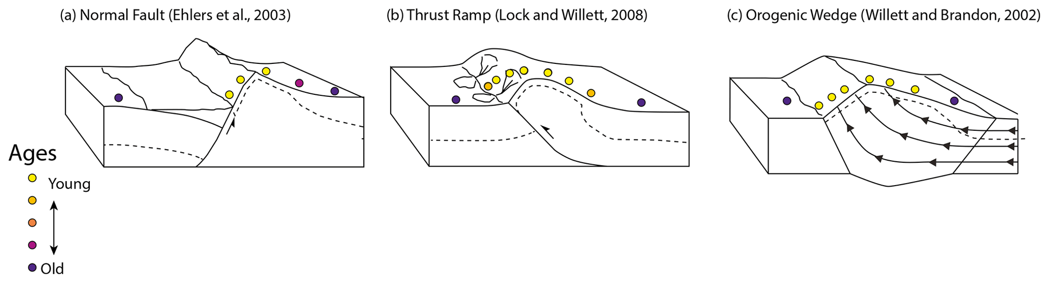
Figure 14Tectonic settings in which thermokinematic modelling has established extensive regions of nearly constant exhumation rates. Dashed line shows an isochron (line of constant age). (a) Normal-fault footwall block (Ehlers et al., 2003). (b) Thrust ramp (Lock and Willett, 2008; McQuarrie and Ehlers, 2015, 2017). (c) Orogenic wedge (Batt and Braun, 1997; Willett and Brandon, 2002; Fuller et al., 2006).
Thrust ramps (Fig. 14b) have also seen considerable attention due to the high exhumation rates and common occurrence of young ages. A number of thermokinematic models have been published based on ramp-flat, fold-fault kinematics (Whipp et al., 2007; Lock and Willett, 2008; Herman et al., 2010; Coutand et al., 2014; McQuarrie and Ehlers, 2015, 2017). These models consistently show that a constant-dip ramp produces a broad zone of constant uplift rate and thus, with a steady surface elevation, a region of constant age. The hanging wall at the lower end of the ramp is typically bounded by a fault-bend fold whose geometry controls the wavelength of a transition from the ramp zone of constant age to the hinterland where there is no exhumation and thus inherited ages. If the up-dip limit of the ramp feeds into a flat, there is a fault-bend fold whose geometry controls the transition from the ramp zone of constant age to the foreland zone of inherited ages. If the ramp reaches the surface and all remnants of the fault-propagation fold are eroded, there can be a narrow zone of older ages in the hanging wall exposed to cooling into the footwall, but otherwise, there is a sharp transition between the cooling zone and inherited ages in the foreland. Gradients in cooling age associated with fault motion are young to old from the centre of the ramp to the thrust but are steep, short and rarely observed in the field.
Orogenic or accretionary wedges have also been much studied, although the complexity of their internal deformation makes it difficult to generalize. One must also differentiate between models that assume a surface erosion rate and allow this to drive kinematics (Dahlen and Barr, 1989; Batt et al., 2001) and those that allow the surface erosion rate to be freely determined with the deformation (Willett, 1999; Batt and Braun, 1997; Fuller et al., 2006; Michel et al., 2018, 2019). Summarizing some of the latter, Willett and Brandon (2002) made the explicit point that within the deforming wedge, rock uplift rates will be constant to maintain self-similar growth and that exhumation rates and ages will also be constant unless some surface process acts independently of the rock uplift associated with wedge growth. Their summary figure included nested reset zones of constant age (Willett and Brandon, 2002) (Fig. 14c). The prowedge of an orogenic belt (right-hand side of Fig. 14c) is characterized by an unreset frontal zone where particle paths are too shallow to permit heating above closure temperatures. The transition to the reset zone can be in either prowedge or retrowedge and can be either discrete, associated with a single structure, or diffuse, often exhibiting partially reset ages, but it is rarely defined by a spatially extensive gradient of reset ages.
The point of these examples is to demonstrate that tectonic activity is not, in and of itself, evidence for spatial variability of thermochronometric ages. All tectonic settings contain extensive domains with constant or near-constant ages. Furthermore, there is a well-known effect of age compression at high rates of exhumation whereby thermochronometric ages become less sensitive to changes in exhumation rate as the rates increase (Ehlers et al., 2001). At high exhumation rates, even large changes in exhumation cannot be resolved by ages with typical measurement uncertainty, whereas temporal differences, i.e. due to changes in elevation or closure temperature, do not suffer from this compression effect. The consequence is that regions with the young ages needed to resolve Plio-Pleistocene cooling have little sensitivity to spatial variations in age and require good temporal coverage, as we will illustrate in the sections below.
5.2 Spatial patterns of exhumation and acceleration: example from the western Alps
Given the insights into potential sources of error in the inverse models (Sect. 4) and tectonic causes of age gradients, or the lack thereof (Sect. 5.1), we turn next to the natural examples to assess where there is potential systematic error. The synthetic models of Sect. 4 were conclusive in showing that there is no model bias but that resolution errors and their amplification through thermal model errors could lead to specific errors. We conduct an analysis of the resolution errors for a number of the original sites, which are specific to each site and data set. In addition, we use these examples to demonstrate problems that arise through the use of the proposed NR metric as an interpretation tool.
The Alps have served as an important example for the application of GLIDE (Fox et al., 2015, 2016; Schildgen et al., 2018), so we will continue this focus here. Figure 15 shows the GLIDE inversion estimate of exhumation rate, together with resolution metrics and the normalized erosion rate difference. The ages used in the inversion are shown in Fig. 15l. They are also shown in Fig. 15a–i, plotted within the time interval into which they fall, to give a better sense as to which time intervals are constrained. Exhumation rates are well constrained throughout the external Alps, which lie north-west of the Penninic line fault (PLF in Fig. 15). There are numerous ages that fall within the 6 to 0 Ma range as well as older ages in both the external and internal Alps, south-east of the PLF.
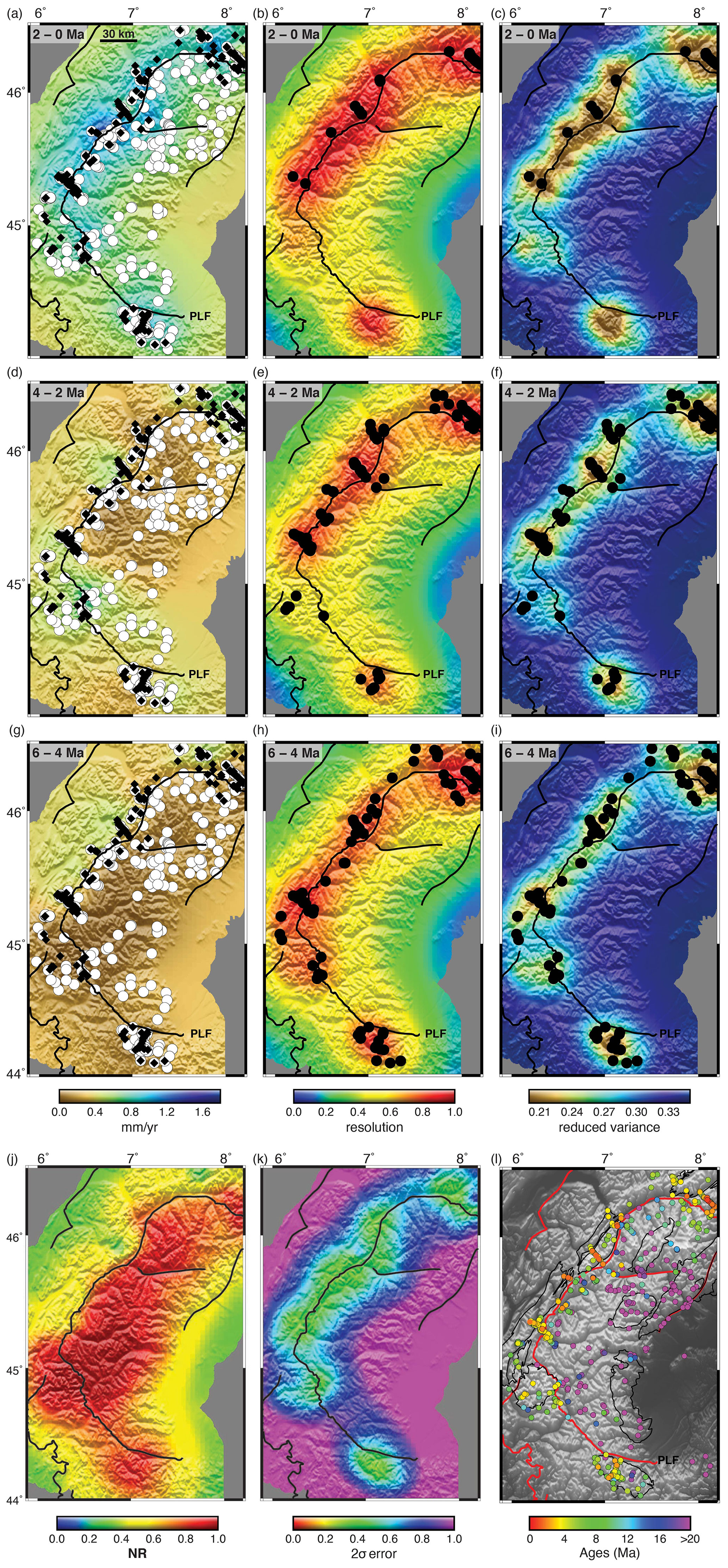
Figure 15Erosion rate history in the western Alps based on analysis from Herman et al. (2013) and Fox et al. (2015, 2016). (a–c) Inferred erosion rate between 2 and 0 Ma, with temporal resolution and posterior variance. (d–f) Inferred erosion rate between 4 and 2 Ma, with temporal resolution and posterior variance. (g–i) Inferred erosion rate between 6 and 4 Ma, with temporal resolution and posterior variance. (j) Normalized erosion rate difference (Eq. 14) and (k) 2σ error in the normalized erosion rate difference (Eq. 16). Inversion parameters are similar to Herman et al. (2013). A prior erosion rate of 0.35 mm yr−1 and a correlation length scale of 30 km have been used. In (a), (d) and (g) the black diamonds indicate ages less than 6 Ma; white dots indicate ages older than 6 Ma. In resolution and variance plots the ages that fall within that time interval are shown as black circles. PLF is the Penninic line fault.
There is a clear increase in erosion rate in the external Alps, closely associated with the young ages. North-west of the Penninic line, exhumation rates are notably higher in the 2 to 0 Ma time interval (Fig. 15a), defining an acceleration with respect to the previous time intervals. The high erosion rates are centred on the high external Alps, where the youngest ages are clustered. This zone of high erosion rate has numerous ages in the 6 to 4 Ma time interval, which is a typical age for the AFT samples from the region. The ZFT ages are older (8 to 16 Ma), and AHe ages are younger than 6 Ma. Erosion rates in this region are thus well resolved across all time intervals.
The good resolution of the Alpine ages can be confirmed by comparison to the model results shown in Figs. 4–9, 12 and 13. To properly make a comparison between the models and the natural example, one must estimate the data density in both space and time and select the model with synthetic data distribution most similar to the natural example. With the data density of the Alps, the closest models are those using Data Set A or E (Fig. 3). Even here, the true age distribution for the Alps is likely better than any age distribution of the models, because the extremely high and sustained erosion rate in half of the synthetic model domain compresses the model ages into a narrow time range. Nonetheless, the models all show that with the data coverage of the natural Alps, we expect only small resolution errors with a very well-resolved history in the external Alps to the north-west, a resolved average erosion rate with no resolution of late change in erosion rate in the internal Alps to the south-east and a smoothed transition between the two.
The region of accelerated erosion south-east of the Penninic line in Fig. 15 is larger than the counterpart in the synthetic models (e.g. Fig. 12). There are several reasons for this. First, the data resolution of the synthetic models and the natural data are not identical, so there are resolution errors throughout the natural example and direct comparison with the model will never be perfect. Second, the uplift functions are very different, and this affects the temporal resolution. The vertical fault with 13 km of relative offset in the synthetic data example makes a good synthetic test, but it should not be mistaken for the actual uplift pattern in the Neogene Alps, which has no major active structures (Egli and Mancktelow, 2013). Finally, and most importantly, the synthetic model and actual Alps differ in that the external Alps do have an acceleration in exhumation, whereas the synthetic model does not. The increase in erosion rate in the external Alps is robust and well resolved by its local ages. Smoothing of this signal from the external Alps during each independent time interval into the surrounding regions, i.e. south-east of the PLF, give the appearance of an acceleration in these regions. The synthetic model had no acceleration in the high uplift region, so any smoothing of the high uplift area into the low uplift area was equal over each time interval.
It should also be noted that even if there were a sharp boundary between young and old ages from the external to internal Alps, it would not be at the Penninic line as portrayed in this paper and Schildgen et al. (2018). There are a number of ages younger than 4 Ma south-east of the Penninic line faults (most clearly seen in Fig. 17e and h), and these extend the high uplift zone to the south. The high uplift zone in Fig. 15a continues south-east into the internal Alps for a distance of less than one correlation length beyond the southernmost young ages. This is the same smoothing effect we observed in the synthetic data models (e.g. Fig. 4 or Fig. 12).
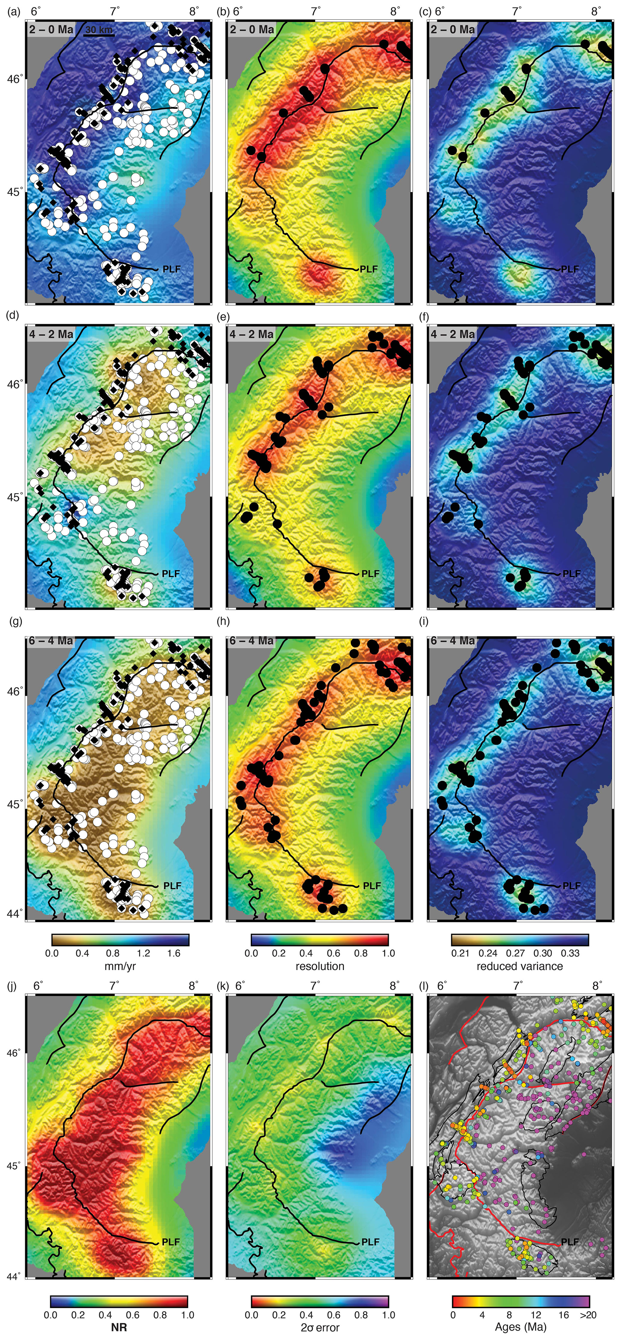
Figure 16Erosion rate history in the western Alps based on analysis from Herman et al. (2013). The model is identical to that of Fig. 15 except that the prior erosion rate is taken to be uniform at a value of 1.35 mm yr−1.
The NR map (Fig. 15j) gives a very different story. The maximum acceleration is shown in the middle of the study area centred on a region with almost no age data younger than 6 Ma. Furthermore, the high acceleration region is large, covering the entire internal Alps at a value larger than the external Alps, where most of the young ages are found. It is this relationship that was the basis of the conjecture of Schildgen et al. (2018) for inappropriate spatial averaging, as there is no intuitive basis for this large acceleration zone centred on a data gap rather than on the data. However, it is here that the shortcomings of a plot based on the NR ratio emerge. Comparison between the erosion rate maps and the normalized erosion rate difference map show that the two have very little in common. The offset in maximum values is the most obvious, but the extent of the large values of NR far to the south and east is peculiar given the data distribution and the lack of deviation in erosion rates from the prior value of 0.35 mm yr−1 through most of the south-east of the study area. The problem is not in the erosion rate maps; it is apparent only in the normalized erosion rate difference maps. The problem is further clarified by looking at the error associated with the NR (Fig. 15k). It shows that the lowest variance in the NR is centred on the external Alps, where the data density is highest and the erosion rates are best resolved. The variance in NR increases rapidly to the south-east, with high values encompassing most of the internal Alps. The shift of the locus of NR relative to its error and its underlying parameters is a feature of a ratio expression where the quantity in the denominator has a wide range of values. Regions where the denominator is small, i.e. the internal Alps, have a large ratio but also increasing sensitivity to error in the denominator. This effect creates a bias, a bias that is manifested as a false acceleration in regions of low erosion rates.
As with the synthetic data models, a test of the resolution can be provided by checking for sensitivity to the prior model. We reran the Alpine data inversion using a prior erosion of 1.35 mm yr−1 (Fig. 16). As expected, the peripheral regions all have a high erosion rate reflecting the higher prior. However, the central external Alps are almost unchanged, reflecting the high resolution. The high-resolution contours (above 0.5 to 0.6) mark the region that is robust against changes in the prior. The internal Alps to the south-east hold their lower erosion rate because of the older ages. There are also somewhat higher erosion rates at all time intervals in the external Alps. This is a model effect due to a difference in the geothermal gradient between the two models, in response to the increased advection of the early history in the high prior model.
As an even more direct test of the hypothesis that the inferred acceleration is an artefact of mixing regions, we produced another inverse model for the Alps, but in this case, we omitted all the data from the internal Alps in the south-east, thus inverting only the data from the external Alps, similarly to the synthetic data model in Fig. 11. Results are shown in Fig. 17. Comparing the inverse model of all the data (Fig. 17a–c) to the model of just the external Alpine data (Fig. 17d–f), one can see that the solutions in the external Alps are essentially identical, proving that there is no influence of the old ages to the south-east on the erosion rate estimates in the north-west. This result is consistent with what we found in the comparable synthetic data example (Fig. 11).
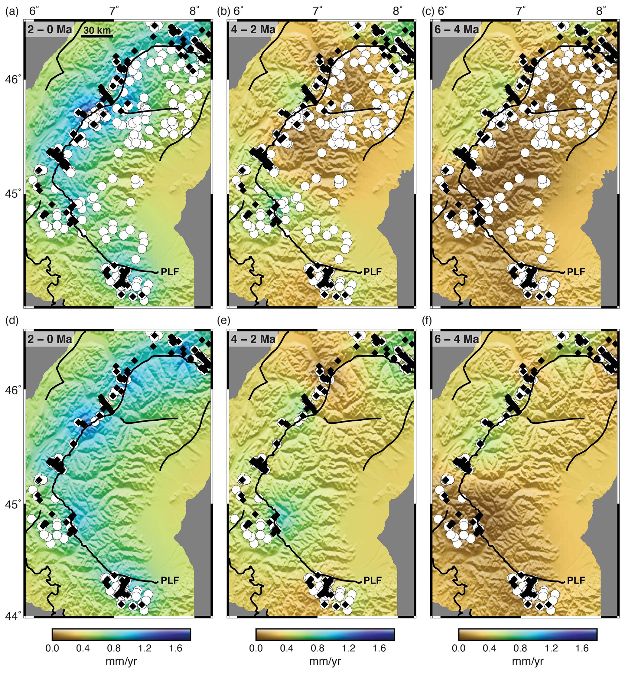
Figure 17Erosion rate history in the western Alps excluding all data south-east of the Penninic line fault (PLF) (d–f) compared to history including all data (a–c) (identical to Fig. 15). All inversion parameters are identical. The erosion rates and observed increase in erosion rates in the external Alps are virtually indistinguishable between the two models, confirming that the solution in the north-western external Alps and the observed acceleration is determined by the local data.
These three models are conclusive; the acceleration found in the Alps is not the product of inappropriate spatial averaging. In the external Alps it is well resolved by the local data which span the time span of interest. In the internal Alps, the erosion rates over this time span are poorly resolved, and so the solution from the north-west is smoothed into this area but not sufficiently that the older ages of this region are misfit.
5.3 Analysis of other natural examples for an increase in exhumation rates
According to the reanalysis of Schildgen et al. (2018), of the 32 sites identified in the Herman et al. (2013) study as showing sufficient thermochronometric data to resolve an erosion rate history over the past 6 Ma, 23 of them were what they called “spurious”. Furthermore, for those cases that were not spurious and many sites that were argued to be spurious, they interpreted the cause as either “tectonic” or “glacial”, where glacial refers to Quaternary changes in erosion rate associated with the onset of glaciation. This second point will be discussed later (Sect. 6.2). The first issue, whether or not results are justified or spurious, will be assessed here. Although Schildgen et al. (2018) applied a variety of criteria as to what constitutes a spurious result, we will focus here only on the question of potential spatial correlation bias, where this is defined as inappropriate spatial averaging of data resulting in a false acceleration.
To clarify how to address spatial averaging and its impact on the conclusions of erosion rate change, we suggest that this should be posed as a set of questions. Are the local data sufficient to resolve an increase or are unrelated data from large distances being used, and is an inferred increase robust with respect to the method of analysis? A spurious result should be limited to an artefact that arises only because of the inappropriate combination of data, model bias, or resolution errors. For the case of a spurious acceleration, a better analysis or knowledge of the “true solution” would reverse the conclusion. This definition does not include smoothing errors if that smoothing includes an area that exhibits a true acceleration based on its local data. Smoothing errors are easily recognized and, if removed, either by a better analysis or simply masking parts of the domain, the conclusions would be unchanged; an acceleration would be inferred in any case. In this sense, results are not regarded as being area dependent; the definition of an artefact must apply to the best-resolved parts of the study area, not just peripheral regions. Thus, the errors in Fig. 10a and b would constitute a spurious acceleration, but the acceleration inferred for the transition between the external and internal Alps in Figs. 15–17 would not be regarded as spurious because it would not arise without the existence of a neighbouring region with a resolved and true increase in erosion rate.
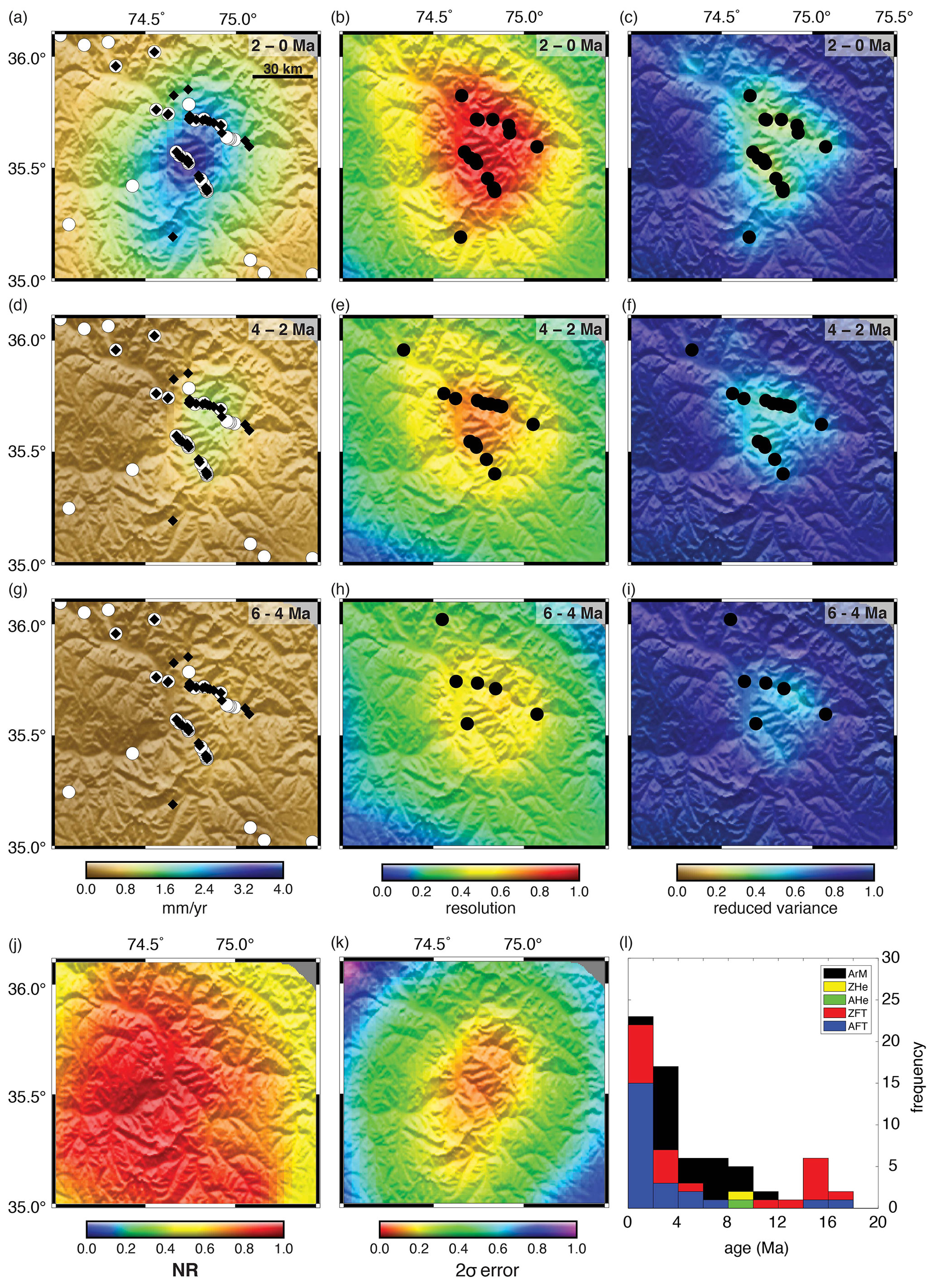
Figure 18Erosion rate history for the western Himalayan syntaxis in the region of Nanga Parbat. Estimate based on analysis from Herman et al. (2013). Inferred erosion rates (a, d, g) for three time intervals, from 6 Ma to present, shown along with the temporal resolution (b, e, h) and reduced variance (c, f, i). (j) NR and its associated error (k) are also shown. (l) Histogram shows age distribution broken out by the thermochronometric system. Inversion parameters are similar to Herman et al. (2013). Erosion rate plots include ages less than 6 Ma as black diamonds and ages greater than 6 Ma as white dots. Resolution and variance plots include the ages that fall within the respective time interval. An inverse model with all data from outside the massif omitted is shown as Fig. A7. There is no appreciable difference in the result.
The previous section presented the Alps as an example of this reanalysis. As a second example of site interpretation, the Nanga Parbat region of the western Himalayan syntaxis is analysed, with results shown in Fig. 18. In order to understand how resolution arises, we have plotted the age data in different ways. First, the full age distribution is shown as a histogram (Fig. 18l). This shows that there are five thermochronometers with ages bracketing the time span of interest. It is important to show how many ages bracket each time interval, so these are shown in the resolution and variance plots. All ages greater than 6 Ma are shown in white on the erosion rate maps, values less than 6 Ma as black diamonds. Taken together, these maps give a good sense as to which data are constraining which erosion rates. The fact that the resolution and variance plots mirror the data reflects local support of resolution. These figures miss the additional resolution provided by elevation range, but this information can be visualized indirectly from dispersion in the age histogram. Figure 18 shows that the core region of the Nanga Parbat syntaxis is well resolved by the local data. With five thermochronometers yielding ages under 10 Ma, the resolution of the exhumation history is excellent. There are older ages outside the massif, so to confirm that these are not inappropriately influencing the solution, we removed all ages from outside the syntaxis core and reran the inversion. Results are shown in Fig. A7 and are essentially unchanged. We could also change the prior model or the correlation length and the conclusions would be unchanged. The acceleration is the result of effectively co-located data from five thermochronometric systems and is not an artefact of the method or of inappropriate averaging, and so by our definition it is not spurious. This result is consistent with the model of Fig. 11, which shows that with data coverage of this density, old ages from other regions have no influence on the solution in well-resolved regions. The region with resolution above a value of 0.4 or perhaps 0.5 includes all the ages less than 6 Ma and none of the region with no ages under 6 Ma and would be regarded as well resolved. In contrast, the map of NR has lost all the information regarding resolution (Fig. 18j). It shows simply a broad, long spatial wavelength increase. However, the error on NR shows that the resolved part of this map is also restricted to the Nanga Parbat core region (Fig. 18k). This region also shows a clear increase in erosion rate with time. We also note that previous studies using different approaches found the same result, including this increase in rate (Zeitler, 1985; Thiede and Ehlers, 2013).
A third example with good spatial and temporal coverage is the Olympic Mountains of north-western Washington State (Fig. 19). Here there are three thermochronometers providing coverage of the 10 Ma to present-day time span and a fourth providing a longer timescale average rate. These data are dominantly from the central core of the mountain belt with older, largely unreset, ages found in the western region where it has been argued that the combination of lower erosion rates and shallow particle trajectories through the orogenic wedge result in a frontal unreset zone (Brandon et al., 1998; Pazzaglia and Brandon, 2001). The GLIDE inversion delineates a well-resolved circular region in the core of the mountain belt centred on the data, with ages falling into all three time intervals. The region is resolved by local data and, as the synthetic models show, with resolution at this level, old ages far removed from the resolved region have no influence on the erosion rate history (Fig. 11). The Olympics provide a particularly good example of the distortion that occurs through application of the NR operator. The NR field (Fig. 19j) shows maximum values offset to the north-west relative to the data. This is an artefact of the division operator, as shown by the error on the NR which remains centred on the data. Consideration of the NR map in isolation could lead to the interpretation that the acceleration is a consequence of spatial averaging, but this would be incorrect.
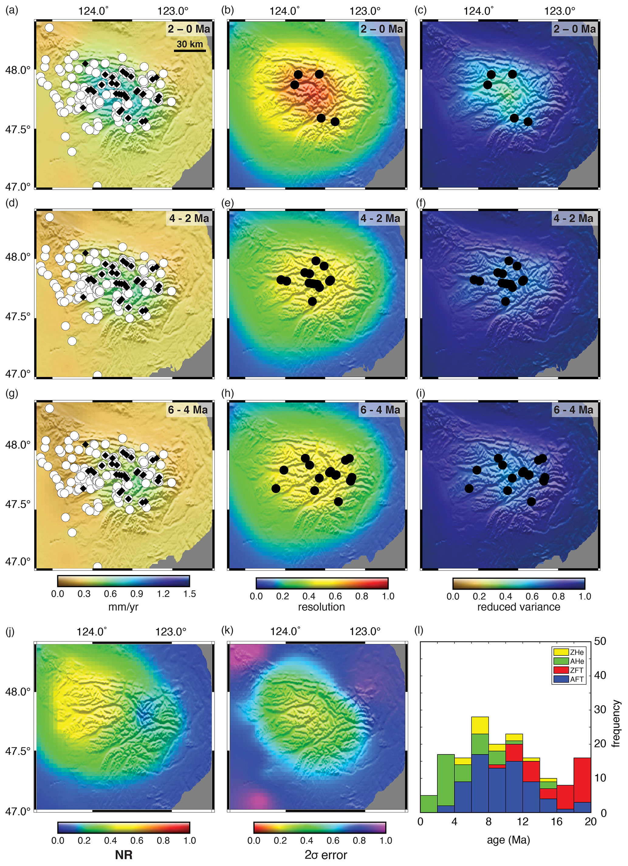
Figure 19Erosion rate history for the Olympic Mountains of north-western Washington State, USA. Estimate based on analysis from Herman et al. (2013). Inferred erosion rates (a, d, g) for three time intervals, from 6 Ma to present, shown along with the temporal resolution (b, e, h) and reduced variance (c, f, i). (j) NR and its associated error (k) are also shown. (l) Histogram shows age distribution broken out by thermochronometric system. Inversion parameters are similar to Herman et al. (2013). Erosion rate plots include ages less than 6 Ma as black diamonds and ages greater than 6 Ma as white dots. Resolution and variance plots include the ages that fall within the respective time interval.
As a fourth example, the Marlborough region of New Zealand (NZ) is one of the most complex tectonic settings considered in these studies. This complexity leaves much latitude for interpretation. In addition, the data are sparse, with only two thermochronometers applied in the region (Fig. 20). The tectonic complexity includes changing rates of fault slip on a system of oblique but dominantly strike-slip faults, which could result in local changes in erosion rate that are not characteristic of the region as a whole. The youngest AFT ages are all found south of the Wairau and Alpine faults and north of the Hope or even Clarence faults (see Schildgen et al., 2018, Fig. S16). These are supplemented by a handful of ZFT ages in the 2 to 10 Ma range. In fact, there are three distinct local areas where there are nearly co-located ZFT and AFT of the correct age to constrain the erosion rate history from 6 Ma to the present; these are visible as the three nearly co-linear points in the 6 to 4 Ma resolution or variance plots of Fig. 20. Not coincidentally, the best resolution and variance reduction occurs along an axis connecting these three points (e.g. Fig. 20k). The two southern points sit on a common tectonic block and the northern point on a second block. However, the data on each of these blocks are sufficient to resolve an erosion rate history with no contribution from data points outside these blocks. This case is thus analogous to the models of Fig. 4 or Fig. 12, where there are two adjacent blocks, one with a good distribution of ages from multiple thermochronometers and one with only old ages. Just as there was no averaging across the fault in those models, we see little evidence for averaging across the fault in this natural case. An appropriate threshold for the resolution and reduced variance would both be about 0.5 to capture these three regions and only these regions with no major inclusion of the other tectonic blocks. Again, the NR is diffuse, broad and offset from its error, so it does not reflect the important characteristics of the inverse model result. In contrast, the correct threshold value of the resolution (0.5) or, even better, a similar value of the reduced variance would nearly follow the block-limiting faults.
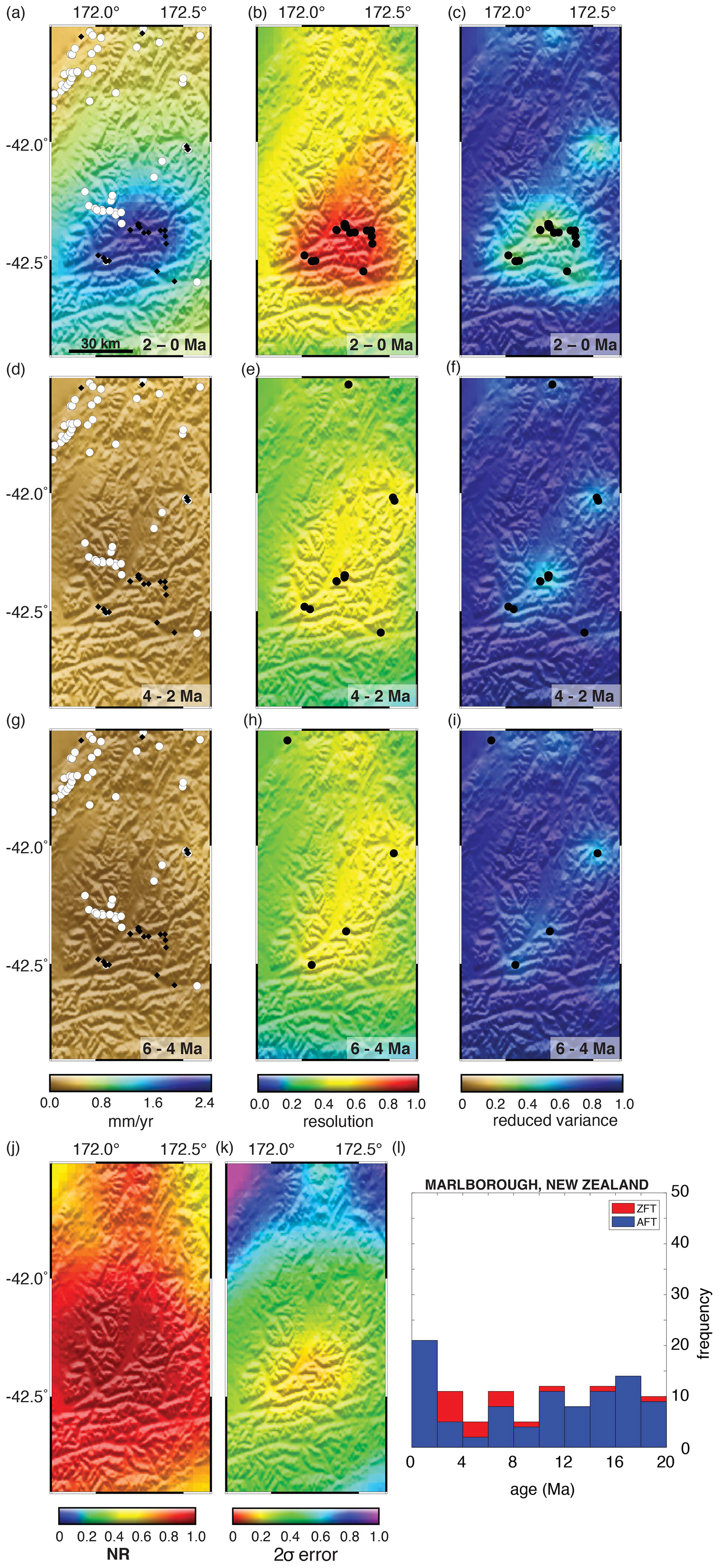
Figure 20Erosion rate history for the Marlborough region, New Zealand. Estimate based on analysis from Herman et al. (2013). Inferred erosion rates (a, d, g) for three time intervals, from 6 Ma to present, shown along with the temporal resolution (b, e, h) and reduced variance (c, f, i). (j) NR and its associated error (k) are also shown. (l) The histogram shows age distribution broken out by thermochronometric system. Inversion parameters are similar to Herman et al. (2013). Erosion rate plots include ages less than 6 Ma as black diamonds and ages greater than 6 Ma as white dots. Resolution and variance plots include the ages that fall within the respective time interval.
The important point illustrated by this NZ example is that it is the existence of collocated ages from different thermochronometers that increases the resolution to the point that we would interpret them as a well-constrained erosion rate history. There are several regions to the north and south of the resolved region that also have a number of ages under 6 Ma, but these regions have exclusively AFT ages, and ages from a single thermochronometric system are insufficient to bring resolution into an acceptable range. It is the sampling of different closure temperatures at different times that determines the resolution and the erosion rate history. It is not a combination of ages from a single thermochronometer sampling different erosion rate histories from across the entire region. Instead, we see most of the region at or near the prior value, with the exception of the tectonic block between the Wairu and Hope faults, which shows rapid uplift in the last 2 Ma. Again, we conclude that there is no spurious acceleration as an artefact of the method. The predicted model is consistent with all the ages, the predicted accelerated uplift is limited to one or at most two tectonic blocks, and the data constraining that history are identifiable and have a common history.

Figure 21Erosion rate history for the Fiordland region of New Zealand. Estimate based on analysis from Herman et al. (2013). Inferred erosion rates (a, d, g) for three time intervals, from 6 Ma to present, shown along with the temporal resolution (b, e, h) and reduced variance (c, f, i). (j) NR and its associated error (k) are also shown. (l) Histogram shows age distribution broken out by the thermochronometric system. Inversion parameters are similar to Herman et al. (2013). Erosion rate plots include ages less than 6 Ma as black diamonds and ages greater than 6 Ma as white dots. Resolution and variance plots include the ages that fall within the respective time interval.
As a fifth and final example, we consider the data from the Fiordland region of New Zealand (Fig. 21). In contrast to the Marlborough region, the data coverage here is excellent, with widely distributed AFT and AHe ages, most of which are younger than 10 Ma, as well as some older ZFT and ZHe ages. The ages fall nearly uniformly across the centre of the region within all three time intervals of interest (Fig. 21), resulting in resolution values approaching 1.0 in many places within all three time intervals. A threshold resolution value of 0.5 would enclose the region with data; a slightly smaller number would include more of the surrounding areas but would not change the interpretation. The NR is again offset from the data, with the locus of its largest values shifted to the south-east, so any direct interpretation of its spatial distribution would be misleading. There is some structure to the erosion rate pattern, for example higher rates in the north across the full 6 Ma interval, but in general the erosion rates are regionally consistent and show an acceleration in the last 2 Ma. This result is based on local ages, is resolved by the temporal distribution of ages from four thermochronometers and cannot be considered spurious.
6.1 Bias, errors and resolution in GLIDE
The central question investigated in this paper is whether there is a systematic error in the methodology of Fox et al. (2014) and Herman et al. (2013) that resulted in an apparent acceleration in inferred erosion rates. As we argue above, this question can only be addressed if one identifies the source of errors within the analysis. We have dissected the possible source of errors and shown that, neglecting measurement errors, which should not be systematic, there are three potential sources of error: (1) model errors due to the parameterization including spatial correlation smoothing; (2) model errors due to incorrect prediction of the near-surface geotherm; and (3) resolution errors that result from inadequate data coverage of space and time. The synthetic data forward-inverse models presented above show that (1) do not exist in any important form, although they are evident in smoothing of sharp boundaries, that (2) are a potentially serious source of error in erosion rates but do not predict a systematic tendency towards acceleration, and that (3) can be large but depend on the individual data distribution as well as the prior model parameters and also have no generalizable tendency towards acceleration.
Resolution errors are the result of data inadequacies, primarily in time, where multiple thermochronometric systems or elevation dispersion are needed in order to give a range of ages adequate to resolve a temperature history. Although every data set has a unique distribution and therefore unique resolution errors, we were able to make some generalizations through analysis of a range of data examples. First, we found that with a large number of data, distributed appropriately in age, all errors, including resolution errors, go to 0. In fact, it did not require a particularly large number of data to obtain excellent estimates in our tests, provided the age coverage is appropriate (Fig. 9). Nor was there any evidence for inappropriate spatial averaging in high-density models. There was smoothing of sharp boundaries, but even here, this occurred primarily where data were insufficient to resolve the boundary. As data density decreases, resolution errors become larger. If data are too few, there are large resolution errors, not surprising as data are required to resolve complexity in either space or time. The distribution of data in time is much more important than the distribution in space, at least with relatively simple patterns of erosion rate (compare Figs. 7 and 8). Errors in the analysis with sparse data followed a specific pattern. Areas with poor resolution and no older ages revert to the erosion rate values of the Bayesian prior model. Regions with poor resolution but older ages take a solution steady in time and consistent with the integral constraint provided by the older ages. As data are added to the inversion, the solution is always a balance between the prior model and the erosion rates needed to fit the data. The resolution matrix and its integrated value reflects the weights given to the data relative to the prior. If the prior is equal to the true rate, there is no error (Figs. 6 and A6). Distal data play a minimal role in this averaging process. The weighting between fitting the data and remaining near the prior is set by the parameter variance. Overfitting to the prior model is evident in data residuals.
The idea that spatial differences in age, i.e. a combination of old and young ages from distinct regions, will always, or even frequently, combine to produce an apparent increase in erosion rate is false. Models in this paper were consistent in demonstrating this point. The reason why this argument fails is that there is no temperature history that can fit multiple data that have different ages but the same distance to the closure isotherm (a combination of closure temperature and sample elevation). An inverse method based on optimization of age prediction and including variable exhumation in both space and time will therefore favour spatial variability over temporal variability. With reference to Fig. 2d and e, a model with spatially variable erosion rates can fit all ages perfectly, but there is no common exhumation history that can fit all ages by including excessive and false changes in time. An exhumation history forced to combine disparate ages but optimizing fit to the ages might tend towards lower rates in the early history and higher rates in the later history, dependent on the fitting criterion, but it will never fit the ages well. This points to the importance of using data residuals to test for model bias as shown in the example of Fig. 10. If there is significant spatial averaging or excessive weighting of the prior model, the ages are badly fit. A model that fits all ages well can only do so by accurately resolving spatial variations in erosion rate. The GLIDE method, based on the soft constraint of spatial correlation but designed to optimize age fit, has a strong statistical tendency towards spatial variation rather than temporal variation.
Given that resolution errors are the primary concern with thermochronometric data modelling, it is important to quantify resolutions for specific data sets and estimate resolution errors. For this reason, much of the study of Herman et al. (2013) and related papers (e.g. Fox et al., 2015, 2016; Jiao et al., 2017) has estimated resolution errors, investigated sensitivity to the prior model parameters (see the Supplement to Herman et al., 2013) and developed new statistics such as the temporal resolution matrix as an integral of the resolution kernel (Fox et al., 2014). The synthetic models in this paper show that the resolution metrics do a good job in delineating relative resolution. Resolution remains a relative measure, and determining a precise confidence level a priori is not possible but can be estimated based on spatial patterns, the relationship with sample locations, fit to the age data and sensitivity to the prior. As a relative measure, resolution scales with other parameters, including correlation length and assumed prior variances.
Although resolution errors do not tend to produce a false acceleration, there are combinations of data and prior model that can lead to a false acceleration. For example, in the case of isolated young ages, less than 2 Ma, with a low prior, the young ages give a high rate of erosion in the last time interval, and if there are no higher closure temperature data nearby, the earlier time intervals will take a value near the prior, leading to an apparent acceleration. However, the early time intervals will not be well resolved, so this should be recognized for what it is, a mix of resolved and unresolved time intervals. The danger is that the resolution does not have an absolute level, so there is a chance that early time intervals will be at the margin of acceptable, even though the constraining data are either too old or too far away to constrain the erosion rate well. For this to occur it requires an unfortunate combination of ages in both space and time. Ages must have a very specific distribution in order to raise the resolution value but not pull the erosion rate away from the prior value. The danger of this combination was recognized by Herman et al. (2013), which is in part why Herman et al. (2013) made a comparison of the 6–4 Ma time interval and the 2–0 Ma time interval rather than the 4–2 Ma time interval and the 2–0 Ma time interval. Comparing the last two time intervals is easier and would still make the point that Quaternary climate change might have impacted erosion rates. However, it is much more difficult to resolve two time intervals with a gap between them, so the 6–4 Ma time interval was used in order to make a more conservative estimate of potential accelerations by imposing a stricter condition on the resolution.
One case that we did not present in the modelling study was the extreme poor resolution that results when all data come from a single thermochronometric system. We have conducted simulations to evaluate this, but the results were as one would expect. It is impossible to find a resolved temperature history with a single thermochronometer, with the exception of a fortuitous elevation distribution, in which case the estimate is both resolved and accurate. This is not surprising. When a thermal model is used as the basis of the analysis and all ages have a common closure temperature, there is no means of resolving more than one point in time, as can easily be recognized by the principles shown in Figs. 1 and 2 and shown in Herman et al.'s (2013) Fig. ED3. This is why most sites identified by Herman et al. (2013) as having sufficient resolution have ages from more than one thermochronometer, and those that do not have an advantageous elevation distribution.
The other major source of error in forward and inverse modelling of thermochronometric data is in the determination of the crustal geotherm. Erosion rates derived from thermochronometric data depend on the geothermal gradient just as strongly as they depend on the measured age (Moore and England, 2001; Ehlers, 2005; Reiners and Brandon, 2006; Willett and Brandon, 2013), so it is essential that thermal models are accurate. By linking the thermal advection in GLIDE to the erosion rates derived from the ages, geotherm errors become part of the model errors in the tests of this paper. Geotherm errors were occasionally large in the synthetic data models, although this was in part a consequence of the extreme erosion rate scenario used in these tests and the fact that the true model was often far from the prior. This leads to a large error in the geotherm if old ages do not exist to constrain advective heating. An acceleration or deceleration as determined by multiple thermochronometers depends, not on the gradient, but on the curvature of the geotherm. A false acceleration would be obtained if the predicted geotherm has less curvature than reality (England and Molnar, 1990), but a systematic error in the gradient affects all rates equally and therefore does not lead to a false acceleration. This effect was demonstrated in Fig. 12, where the gradient was too low, so the estimated erosion rates were too high, but there was no false acceleration. In fact, the error produced a false deceleration.
Transience in lithospheric geotherms is a consequence of many geodynamic and surface processes. Crustal thickening or thinning lead to downward and upward advection, respectively, as well as changes in the distribution of heat production within the lithospheric column. Erosion leads to upward advection of heat. These transient states of the thermal lithosphere persist for tens to hundreds of millions of years, reflecting the timescale of equilibration of the thermal lithosphere (Sclater and Francheteau, 1970; McKenzie, 1978; England and Thompson, 1984; Furlong and Chapman, 2013). Modelling methods sometimes approximate lithospheric transience with a thermal boundary condition at a shallower depth in the lithosphere, often because of computational limitations, but this should always be recognized as an approximation. A basal boundary condition can be either a constant temperature or constant gradient (also referred to as a constant flux condition based on Fourier's law) and can be applied at a material point, e.g. at the base of the crust, which moves up or down with time, or at a spatial point, e.g. at a constant depth. A constant gradient has the advantages that the time to a new steady state is longer than the fixed temperature approximations and is therefore closer to that of the full physical problem. The constant gradient and material point boundaries have the advantage that advective heating or cooling through the boundary is approximated, by changing temperature in the former, and changing position in the latter, making these appropriate conditions to be applied in the shallow lithosphere. The worst approximation is a constant temperature applied at a constant depth. A fixed temperature suppresses advective heat flux across the boundary, so that if applied at a shallow depth in the lithosphere, energy is not conserved within the lithosphere, the geothermal gradient is suppressed and the timescale of transience is greatly reduced.
The 1D thermal model of GLIDE will fully account for the transience due to vertical advection in response to surface erosion. With erosion rate as a general function of space, it is also capable of resolving lateral variations in exhumation in response to spatial variations in tectonic displacements. The model misses lateral conduction of heat, but given that this becomes important only very close to faults with high and sustained rates of displacement, this is a small restriction on solution validity.
In practice, avoiding geotherm errors in thermochronometric studies is best done by estimating and incorporating the modern geothermal gradient obtained by heat flow studies and (if available) other geologic evidence for pressure–temperature conditions at depth. If the final geotherm from the inverse model is calibrated to the observed final geotherm, errors at the time of age closure will be small, even with a simplistic thermal model.
6.2 Summary of problems in Schildgen et al. (2018)
The primary hypothesis of Schildgen et al. (2018) is that there exists a “spatial correlation bias” in all the results of Herman et al. (2013). The analysis above found no evidence for systematic bias, so it is important to evaluate why Schildgen et al. (2018) came to such different conclusions.
Schildgen et al. (2018) presented a series of forward-inverse model experiments similar to those presented in Sect. 4 of this paper. However, those models all showed large errors throughout the spatial domain that were not evident in the results of our experiments. The data sets were not identical in terms of data locations and the values of the ages, so resolution varied between models but not sufficiently to account for the large differences, particularly as we presented a range of models with varying resolutions. The source of the discrepancy lies in the way in which Schildgen et al. (2018) calculated the thermal histories and ages used for the experiment. Schildgen et al. (2018) used an independent model to generate the synthetic data (Pecube, Braun et al., 2012) and a second model to invert those data in their model tests (internal GLIDE thermal model, Fox et al., 2014). Both codes include advection, conductive heat transport and a 3D representation of surface topography and so are capable of reproducing identical results. However, Schildgen et al. (2018) applied different boundary conditions in the forward and inverse models. In the forward model using PECUBE, they applied a constant temperature boundary condition at 30 km, whereas GLIDE uses a constant flux boundary condition. These are fundamentally different conditions and result in different geotherms. By using one geotherm to generate synthetic age data and a second geotherm to invert those data, it becomes impossible to recover the original exhumation rates.
To demonstrate the importance of constant temperature vs. flux boundary conditions, we calculate geotherms using the parameters Schildgen et al. (2018) used for their first example, the western Alps, although the conclusions apply to all tests. The differences in a 1D version of these two models are shown in Fig. 22, which includes the same initial geothermal gradient and exhumation rate of 1 mm yr−1, appropriate for the high erosion rate region of the model. With such a high exhumation rate, the geotherm in the Pecube model has reached steady state by 20 Ma but at a low average gradient suppressed by the fixed temperature boundary condition which restricts the advective heat transport from the mantle. In contrast, the flux boundary condition predicts a higher average geothermal gradient and remains in a transient state as the temperature in the lower lithosphere has not yet reached its final value. The difference in the depth to the closure temperature for all low-temperature systems is up to several kilometres.
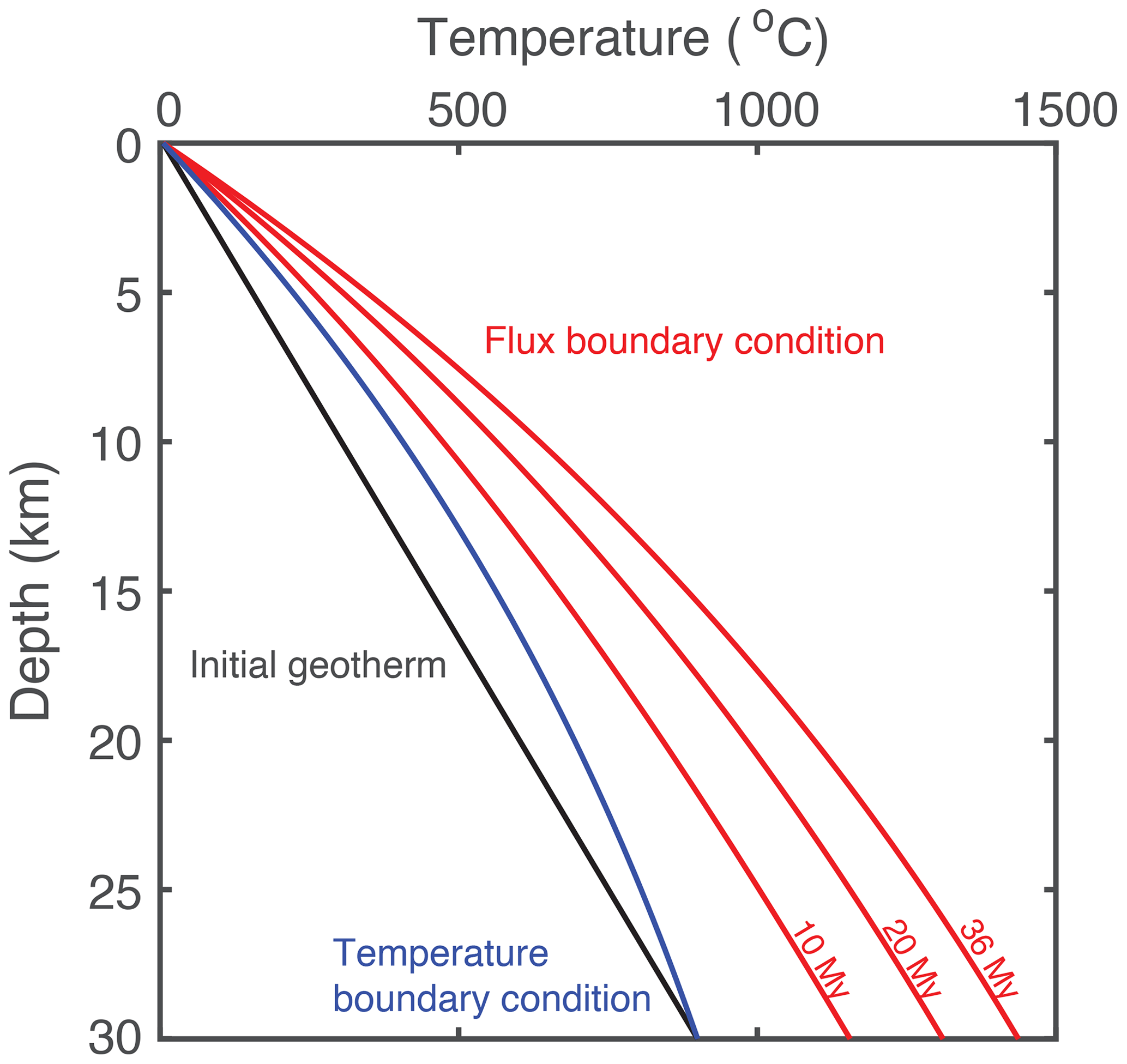
Figure 22Influence of the basal boundary condition on the geothermal gradient. (a) Two models are shown. Both initiate at a constant gradient (black) and with identical thermophysical properties. The blue line is the geotherm after 20 Myr assuming an exhumation rate of 1 mm yr−1 and using a fixed temperature at a depth of 30 km. By 20 Ma, the geotherm has reached a steady state. The red lines are the transient geotherms for an exhumation rate of 1 mm yr−1 and using a flux boundary condition applied at 30 km. Steady state will not be reached for another ca. 50 Ma. In GLIDE, ages are predicted on one of the red curves through the course of the model run. Schildgen et al. (2018) used synthetic ages calculated using the blue geotherm, inverted them using temperatures predicted from the red geotherms, and concluded that the failure to recover the correct exhumation rate demonstrated a problem with spatial correlation in the GLIDE inversion method.
To illustrate the age disparities that result from such different basal boundary conditions, we regenerated the ages using the exhumation rates of the Alps synthetic model but using the thermal model assumptions made in GLIDE, assuming a flux boundary condition and a total length of time of 36 Myr. We calculated the ages for both high and low uplift rate regions. The predicted ages are significantly different (Fig. 23), with the Schildgen et al. (2018) ages systematically older by up to a factor of 2. This difference is due to the lower thermal gradient and deeper closure temperature depths predicted from a constant temperature boundary condition (compare blue and red curves in Fig. 22). In addition, the systems with higher closure temperatures are affected more strongly, and the magnitude of the error increases.
Figure 23Comparison between ages predicted with Pecube using a constant temperature boundary condition at 30 km (Braun et al., 2012) and GLIDE (Fox et al., 2014) using a flux boundary condition at 30 km. The ages were generated assuming the same exhumation rates (i.e. 1 mm yr−1 north-west of the Penninic line fault and 0.25 mm yr−1 south-east of the Penninic line fault). Green points are AHe ages, blue points are AFT ages and red points are ZFT ages. The two exhumation rate zones are represented by circles (1 mm yr−1) and diamonds (0.25 mm yr−1), respectively. Outliers in the lower-right corner were likely placed on the wrong side of the fault in one of the models and were removed from the inverse analysis.
The use of different thermal models for the forward and inverse models invalidates this exercise as conducted by Schildgen et al. (2018). The inverse model will do a good job in fitting the ages, but it can only do so by producing the “wrong” erosion rate. Furthermore, because the errors in the synthetic ages have increased bias, that is, they get systematically larger with increasing closure temperature, the inversion is likely to infer an increase in erosion rate with time in order to fit these ages. The impact on GLIDE-inferred erosion rates from these age errors cannot be assessed exactly because of the coupling between erosion rate and advection. The error in the ages results in an error in the advective heat transport, so the resultant geotherm will differ from that of Fig. 22, but it is clear that the errors will be large, and it is no surprise that the results presented in Schildgen et al. (2018) ED Figs. 3, 5 and 6 show large errors. However, rather than being an artefact of the inversion methodology or an effect of spatial averaging of erosion rates, this is an inevitable consequence of introducing a large methodological error into the experiment design by calculating ages incorrectly. This is confirmed by the fact that the experiments conducted above (e.g. Figs. 4, 7, 9, 11 and 12) show nothing comparable to the errors in Schildgen et al. (2018).
The second part of the Schildgen et al. (2018) critique was a reinterpretation of the age data and the Herman et al. (2013) results through their proposed NR maps. This analysis is also problematic because of the problem discussed above with the use of a ratio in evaluating two values with errors. The division of two random variables is a biased operation, and this bias is towards larger numbers as the denominator becomes small. The methodology used by Schildgen et al. (2018) was thus to take the results of Herman et al. (2013), reprocess them using a biased operator (NR), identify that the resultant map contains bias and conclude that the original analysis was flawed. Furthermore, because they did not propagate uncertainty through their NR operator, they lost all relative and absolute uncertainty. The NR bias has a tendency to shift the locus of the largest values of acceleration towards regions with low average erosion rates because of the effect of division by small numbers. The result is a systematic shift and amplification of the signal found by Herman et al. (2013) (e.g. Figs. 15 to 21), so that the locus of high values always sits offset from the data locations and the best-resolved part of the signal. Some of these regions were likely, incorrectly, included in the Herman et al. (2013) analysis, and the ratio error does skew the final results in Herman et al. (2013) but not enough to change the sign of the signal, as we demonstrate below. The ratio error was much more important to the Schildgen et al. (2018) analysis because their major conclusion, that there exists a spatial correlation bias, was based on an interpretation of the spatial pattern of the NR, a pattern that is badly distorted with respect to the original findings of Herman et al. (2013).
The danger in interpretation of the NR map was illustrated by the example of the Alps (Figs. 15 and 16). The distortion of the NR with respect to the data and the inversion predictions was clear, with the highest values of the NR offset from the data by tens of kilometres. By interpreting the spatial pattern directly, Schildgen et al. (2018) hypothesized that the inversion method was averaging data from the internal and external Alps with their differing exhumation histories. We tested this hypothesis and found it to be false (Fig. 17).
This was not an isolated example. In case after case, Schildgen et al. (2018) interpreted the spatial pattern of the NR in terms of spatial averaging of age data. For the Nanga Parbat region, they wrote that “the linear inversion performed by ref. 6 [Herman et al., 2013] suggests a broad zone of late Cenozoic erosion-rate increases both within and outside the massif. This result is a consequence of combining data from inside and outside the NPHM [Nanga Parbat-Haramosh Massif], across the active bounding fault zones”. We tested this hypothesis (Fig. A7) and again found that it is false. The data local to the Haramosh Massif are sufficient to resolve the full history, including the acceleration, with no need to include data from outside the massif (Fig. A7).
The Olympic Mountains of north-western Washington State provided an example of an increase in exhumation rate resolved by four thermochronometers, co-located in the core of the mountain belt (Fig. 19). However, the NR map shows the largest increases in exhumation rate offset from the data, and Schildgen et al. (2018) directly interpreted the spatial pattern of the NR field, stating that “the global inversion found normalized increases in exhumation rates … with the largest increases in the region with the steepest spatial gradient in ages (Fig. S11c). This difference likely arises because the vertical exhumation paths assumed in the linear inversion model used by ref. 6 [Herman et al., 2018] are inappropriate for this setting, and because data that experienced disparate exhumation histories were combined.” We see the same error made as in the Alps and Nanga Parbat; the largest, well-resolved, erosion rate increase occurs on top of the co-located ages from three thermochronometers, not where the steepest spatial gradients occur. The hypothesized combination of disparate exhumation histories is conjecture based on interpretation of distal, often statistically insignificant, parts of the NR map. The spatial gradient in age is not expected to have any effect on the result as shown by the model in Fig. 11 and in any case is located away from the well-resolved regions. More recent and independent work modelling the Olympic thermochronometric data (Michel et al., 2018, 2019) investigated the effects of 3D thermokinematics and found that results did not differ significantly from 1D models. They found the same acceleration as Herman et al. (2013). The acceleration is real, based on local data, not an artefact, and there is no basis for referring to this result as spurious.
Fiordland, New Zealand, is very similar to a high-density data set sampled across the high-relief mountain range. The data, the inversion result, the resolution indices, and the uncertainty in the NR ratio all indicate a signal centred on the data (Fig. 21a–i and k). Only the NR breaks this pattern with an offset to the south-east (Fig. 21j). In this case, there are not even other data to the south-east to call on for inappropriate spatial averaging. However, Schildgen et al. (2018) still assess this acceleration as spurious, stating that “the broad zone of increased exhumation rates is probably at least partly linked to correlating samples across active (or recently active) faults.”, with “peak values frequently occurring in areas of relatively low relief”, so it is evident that they are putting weight on the large values of the NR rather than focusing on the resolved values, which are directly over the high topography and young ages. Although there may be some effect of faults at short wavelengths (Sutherland et al., 2009), there is no evidence that these would create some fictitious artefact in acceleration rather than simply being averaged as in Fig. 2. Short-wavelength variations provide no explanation for either the observed acceleration or for the offset of the maximum values of the NR with respect to the data. We find no justification for the assignment of “spurious” to the original finding of Herman et al. (2013).
We could continue to discuss each example covered by Schildgen et al. (2018) in their Table 1 and data supplement, but we have reviewed all the sites, and the results are the same as the examples above. In each case, the only evidence presented for a spatial correlation bias is the spatial pattern within the NR map and its relationship with the data distribution.
Although the main concern of this paper is the hypothesized existence of a spatial correlation bias, Schildgen et al. (2018) also discussed other potential issues in the analysis of Herman et al. (2013). Their assessment and attribution of “spurious” to a specific site result in Herman et al. (2013) were based on a mixture of criteria, so the meaning varies from site to site. The classification from their assessment includes the following: (1) data errors through inclusion of inappropriate data; (2) model errors, for example interpreting settings that have 2D kinematics with GLIDE's spatially variable, 1D exhumation model; (3) localized valley incision, rather than regionally constant erosion; and (4) inappropriate spatial averaging. The last is the main topic of this paper. The first, data errors, are certainly present in the Herman et al. (2013) study. With nearly 18 000 data, some are undoubtedly not simple cooling ages. The issue is how many, how to identify them and, most importantly, what impact their removal would have on the Herman et al. (2013) result. The first two issues are challenging, often subjective; the last is a straightforward test, requiring the removal of questionable data and rerunning the inversion. However, Schildgen et al. (2018) did no testing for the importance of data errors. They hypothesized many potential problems but tested none of them, so even if data errors are real, we have no sense of how they impacted the inversion results. Lacking any evidence that they are significant to the GLIDE results, we will not address these in this paper. Model errors due to complex kinematics, exhumation or cooling paths are also suggested to be a source of error, but as with the data errors, no tests of this hypothesis were constructed by Schildgen et al. (2018). To test this would require comparing 2D or 3D thermokinematic models to the spatially variable 1D model of GLIDE for individual sites. Results from such tests are difficult to intuit given that the thermal model in GLIDE is not simply 1D but includes 3D topography effects through an analytical formulation and 2D variation in vertical velocity, advection and diffusion. Missing are only horizontal components of advection and diffusion, and these are typically small compared to the former. Until these tests have been completed, the importance of model errors remains speculative. The models presented above suggest that there is no important impact of spatial gradients (Fig. 11) or age offsets (Figs. 4 to 10) on GLIDE results, at least not independent of the question of data resolution.
Localized valley incision is particularly problematic as a criterion for a spurious increase in erosion rate. Schildgen et al. (2018) argue that because the volume of sediment removed by valley incision is less than that removed by spatially uniform erosion, the Herman et al. (2013) result is “spurious”. However, Herman et al. (2013) made no prediction of sediment yield. Herman et al.'s (2013) predictions were for erosion rate and change in erosion rate at the site of thermochronometric age measurement, with the principal prediction being for the direction of change. Although changes in sediment yield are one of the implications of the Herman et al. (2013) result, it is not the only one. If the Herman et al. (2013) results were exclusively reflecting deep valley incision, they would still be an important metric of a globally widespread change in surface erosional processes and rates, such as an increased importance of valley glacial incision. Most importantly, the occurrence of deep valleys does not invalidate the thermochronometry analysis; erosion rates in the valley remain accurate, even if the valleys are transient and morphologically young (Braun, 2002a). The rates might not apply to the entire landscape, for example to the upper parts of the landscape, but, on average, the erosion rate of the region must increase if the valley incision rate increases, and given that determination of the sign of the change in erosion rate is the primary objective, an overestimation of the affected area has no impact on the conclusions of Herman et al. (2013) or this paper. In our view, the local valley incision identified by Schildgen et al. (2018), rather than being a refutation of the result of Herman et al. (2013), should be regarded as a confirmation that Herman et al. (2013) correctly determined the sign of the change.
It should be noted that, apart from the synthetic data models, which were calculated with the wrong geotherm, Schildgen et al. (2018) is an interpretation, not an analysis. There is no reproducible methodology. It is an interpretation of past studies, including Herman et al. (2013), and an assessment of the raw data. This type of analysis is susceptible to another type of bias, not yet discussed, which is known as confirmation bias. This emerges when some observations are selectively used and others selectively ignored in order to support a preconceived hypothesis. We see ample evidence for this bias throughout the Schildgen et al. (2018) interpretation. Because their working hypothesis was that the increases in erosion rate found by Herman et al. (2013) were a consequence of spatial gradients in ages from single thermochronometric systems, often averaging data from large distances, these conditions were searched for and often exaggerated. This is perhaps most evident in their portrayal of the thermochronometric expression of tectonic structures. In Fig. 14, we presented several settings which have extensive thermokinematic modelling work, establishing age patterns which are best characterized as showing constant or near-constant ages over extensive spatial domains. Schildgen et al. (2018) presented a summary of these same settings in their Fig. 1 but with all figures depicting steep age gradients. These gradients do not appear in the original studies cited above, nor, as far as we can determine, in any of the studies cited in their paper. For the normal-fault model, the shallow gradient reported by Ehlers et al. (2003) is exaggerated to the maximum possible gradient with an isochron perpendicular to the surface, implying footwall tilt, not of the 10 to 15∘ observed, but of 90∘, something that does not occur in this setting. For both the thrust ramp and the orogenic wedge, the zones of constant age have been replaced with a gradient younging towards the bounding ramp. The literature has no support for this gradient. With a thrust ramp there is either no gradient or a slight increase in age due to footwall cooling but never a decrease in age. In fact, the Schildgen et al. (2018) versions of the ramp and wedge settings imply a normal sense of shear across the ramp hanging wall or across the entire retrowedge (a rock at the ramp fault is moving faster than a rock in the orogen interior), and such a strain rate field has never been observed or emerged from a model. The natural settings indicated in their figure are similarly incorrect. New Zealand is not a simple thrust ramp but rather is in a transpressional setting, so the ages do young towards the foreland, but the kinematics are not those of a simple ramp, and any thermokinematic model fit to those ages has had to include more complicated kinematics with multiple blocks or internal deformation (e.g. Beaumont et al., 1996; Herman et al., 2009). The central Himalaya have been much studied, with a number of papers arguing that the ages are constant across the major structural ramp (Burbank et al., 2003; Herman et al. 2010). As with rapidly moving normal faults, this is partially a consequence of compression of the age–erosion rate relationship at a high erosion rate (Whipp et al., 2007; Thiede et al., 2009; Thiede and Ehlers, 2013). For the accretionary wedge model, rather than showing the youngest ages in the retrowedge (Fig. 16f), the Olympics have no reset ages (Batt et al., 2001), the Apennines have distinctly older ages towards the retro-deformation front with the youngest ages in the core of the mountain belt (Thomson et al., 2010b), Taiwan has constant ages (Willett et al., 2003; Fellin et al., 2017), and the Alborz as a transpressional system has no systematic pattern, with most ages unreset (Ballato et al., 2015). Thus, the age gradients depicted in Fig. 1 of Schildgen et al. (2018) and hypothesized in their interpretation are perplexing because a figure intended to illustrate spatial patterns of ages has altered those patterns from the original studies, adding characteristics that do not exist in the original studies. Such bias also exists in their site-by-site assessment, where their interpretation contradicts many previous works using a variety of other analysis methods that found increases in exhumation rate (e.g. Zeitler et al., 1982; Ehlers et al., 2006; Thiede and Ehlers, 2013; Michel et al., 2018; Vernon et al., 2008; Shuster et al., 2005; Sutherland et al., 2009; Thomson et al., 2010a, b; Avdeev and Niemi, 2011; Shuster et al., 2011; Ballato et al., 2015; Bracciali et al., 2016). In each of these cases, the original study results were rejected, and Schildgen et al. (2018) designated the outcome as spurious with little explanation and no objective tests as a basis for this contradiction.
6.3 Climate or tectonics – chicken or egg, revisited
A final and important question in any study addressing the impact of climate change on erosion rate is differentiating between changes in erosion rate due to changes in tectonic processes from changes in erosion rate resulting from changes in climatically modulated surface processes. Although this question is not exclusive to thermochronometry, it remains fundamental to the interpretation of any analysis (Kirby, 2018).
In their study, Schildgen et al. (2018) found that, in cases where there is an increase in erosion rate, none were conclusively climate-driven, and there were no more than two or three that were even potentially influenced by climate change. This is a surprising conclusion, not so much that tectonics appears to dominate, but that such an assessment would even be attempted. Unravelling the effects of tectonics and climate-modulated erosion has been regarded as one of the unsolved challenges in Earth science over the last 30 years and is commonly referred to as the “chicken-or-egg” paradox within the field (Molnar and England, 1990; Zhang et al., 2001; Molnar, 2004). This problem is regarded as a paradox because of the feedback between erosion and tectonic uplift. An increase in erosion rate due to climatic factors leads to an increase in rock uplift due to isostatic unloading. If that uplift manifests itself through surface deformation, tectonics becomes the consequence of erosion, not the cause. The alternative, that internal stress change drives a change in tectonic deformation rate and thus erosion rate, cannot be differentiated from the isostatic response scenario; observations are essentially identical. Erosion rates and tectonic activity are nearly always correlated, but there is no basis to assign cause to one and response to the other because of the strong feedback between deformation and gravitational unloading.
Quantifying tectonic influence on exhumation rates is often conducted using thermokinematic models, which combine models of tectonic displacements with thermal advection–diffusion models in order to predict thermochronometric ages. However, these cannot be used to test the relative importance of climate-change-driven erosion and tectonic-driven erosion. The feedback between erosion and tectonics is based on stress changes in response to erosional unloading, and thermokinematic models have no stress calculations. Stress modelling including the impact of erosion on deformation requires use of a dynamic model, and although these have been applied to tectonics–erosion coupling and thermochronometry prediction (e.g. Batt et al., 2001; Fuller et al., 2006; Bendick and Ehlers, 2014), their inability to predict specific realizations of stochastic processes, such as brittle fault formation, or river basin geometry precludes their use for specific site studies.
For these reasons, Herman et al. (2013) made no attempt to attribute cause to erosion rates or accelerations at any given site. This was regarded as an unanswerable question. Rather, the argument was that there were so many sites that showed an acceleration that a coincidence of a tectonic cause was not likely and Quaternary climate change leading to enhanced erosion rates was a more probable explanation for skewing the direction of the change (Molnar, 2004). Some sites may well have had an increase in tectonic uplift rate, in particular in young mountain belts like Taiwan or the Southern Alps of New Zealand, where there is independent evidence for the acceleration of orogenesis. However, independent proof of the cause of a change in tectonic uplift rate is difficult to obtain and is nearly always circumstantial in nature. There is too much subjectivity involved with such a complex problem, so Herman et al. (2013) simply kept all sites and evaluated the composite. In an unbiased and constantly changing world, half the sites would be expected to show an increase and half a decrease.
In contrast, Schildgen et al. (2018) offered an assessment as to the cause of each change in exhumation rate. They presented no new methodology nor any solution to the problem of establishing cause and effect in a system with feedback. Their paper joins quite a few others that have missed the difference between cause and correlation (Molnar, 1990), but it is surprising that Schildgen et al. (2018) give such a definitive answer to such an elusive question.
Any interpretation of cause is also complicated by the fact that the primary means to date or establish rates of tectonic processes over million-year timescales is thermochronometry. To use thermochronometry to establish tectonic deformation rates to explain thermochronometric cooling rates is circular. There are few other methods to date rates of deformation. In some isolated cases geochronology can be used, for example on syn-tectonic volcanic flows, but really the only independent method capable of resolving tectonic deformation rates across a 5 Ma timescale with enough precision to identify changes in rate is sedimentary growth strata with established bio- or magneto-stratigraphy. These do not exist at any but a handful of the sites studied in both papers because most sites are in highly exhumed, often crystalline-cored mountain belts. An exception is the Alps, where constraints on the tectonic activity in the Alps also come from the peripheral foreland basins, the Molasse Basin, and the Po Basin, both of which show Quaternary rock uplift, indicating that erosion has recently begun to outpace tectonic crustal thickening leading to flexural isostatic rebound (Champagnac et al., 2007, 2009; Willett, 2010). The frontal fold and thrust belts on both sides of the Central Alps ceased motion in the Pliocene sometime prior to 3.4 Ma in the Jura (Bolliger et al., 1993; Becker, 2000) and in the early Pliocene for the Lombardic thrust belt, as evident in growth strata and thrust-sealing post-tectonic sediments of the Po Basin (Fantoni et al., 2001; Willett et al., 2006). The major structures, including the Mont Blanc shear zone, Mont Blanc back-thrust, and Penninic thrust had also ceased motion by the end of the Miocene (Egli and Mancktelow, 2013). The geologic evidence thus points to the cessation of tectonic activity throughout the Alps over the last 5 Ma, at the same time that the erosion rates are increasing in the external Alps. Similarly, the Apennines show a decrease in the frontal-thrust propagation rate over the last few million years, anti-correlated with an increase in exhumation rate (Boccaletti et al., 2010).
6.4 Potential improvements to the study of Herman et al. (2013)
The study of Herman et al. (2013), like any study, could be improved. With the insights of several years of additional work using the inversion method, we have learned much that could be applied to the global assessment (Ballato et al., 2015; Herman and Brandon, 2015; Fox et al., 2015, 2016; Margirier et al., 2016; Yang et al., 2016; Bertrand et al., 2017; Jiao et al., 2017; Siravo et al., 2019; Vincent et al., 2020). However, the substantive changes that we would make would be to the way we handled the post-processing of the results. We see no major problems with the inverse method, but the treatment of the resultant erosion rate fields has some errors.
First, it is worth clarifying what the conclusions of Herman et al. (2013) were. The Herman et al. (2013) study analysed exhumation rates globally but selected only regions that had temporal resolution above a specified limit, primarily requiring a significant number of ages under 5 Ma. This limited the analysis to sites with high erosion rates, most of which are tectonically active. The null hypothesis tested by Herman et al. (2013) was that these specific regions, individually or collectively, have had no change in erosion rate over the past ca. 5 Ma. The analysis was applied to age locations but then transferred to a set of regularly spaced grid points for visualization. They found that over 80 % of sites with sufficient resolution had experienced an increase in erosion rate over the past 6 Ma. It is important to note that such an analysis does not provide global erosion rates and was never intended to provide an estimate of global erosion rates over any time frame. A correlation with global climate change and global sediment flux was made under the explicitly stated assumption that the high erosion rate, mountainous areas make a significant contribution to global rates. This comparison was made in time but not by volume.
In post-processing results, Herman et al. (2013) summarized the magnitude of the change in erosion rate by taking two time intervals (6–4 and 2–0 Ma), taking their ratio on a point-by-point basis and compiling their distribution into a histogram (Herman et al., 2013, Fig. 2). This approach is subject to the same ratio bias as the normalized difference used by Schildgen et al. (2018). A ratio analysis should not be used when the goal is to estimate the magnitude of a change, the range of values and uncertainty is large and some values are approaching 0.
This bias is avoided by using a difference instead of a ratio. We demonstrate this by recalculating the change in erosion rate found by Herman et al. (2013), replacing the ratio of the 6–4 Ma time interval and the 2–0 Ma interval with a simple difference between the two (Fig. 24). We have done this for three values of the resolution cut-off, all larger than the 0.25 used in Herman et al. (2013). The principal effect of the change to a difference is to truncate the distribution reported in Herman et al. (2013) by removing the largest values. These large values were the consequence of small but uncertain numbers in the denominator of the ratio. However, the general form of the distribution and the positive mean remain the same as in Herman et al. (2013). The principal result of Herman et al. (2013) is thus unaffected by this bias.
Figure 24Recalculation of the global change in erosion rate between 6–4 and 2–0 Ma from the inversion results of Herman et al. (2013). Change is expressed as the difference between the erosion rate inferred for each of these time windows. Results are shown using three values for the resolution cut-off, from 0.3 to 0.5.
Resolution and other posterior variables depend on a wide range of data parameters and inverse model parameters, so their absolute value is often scalable. In particular, they are subject to the well-known trade-off in inverse theory between resolution and variance reduction. To reduce the effects of noise in the data, resolution is sacrificed through spatial averaging. The trade-off is between a well-resolved average parameter and a poorly resolved local parameter. High resolution corresponds to less reduction of noise variance. The degree of regularization of the model also comes into the absolute values of the resolution and variance. This comes primarily through the damping that occurs by setting a noise variance on the data (Eq. 3). The regularization is determined by the ratio of the noise variance and the prior parameter variance.
As the resolution cut-off is increased, the number of resolved points is reduced (Fig. 25). With a cut-off value of bias of 0.5, there are fewer than 200 points worldwide. However, these remain distributed globally, and a resolution cut-off of 0.4 gives over 500 points with a much broader spatial distribution. The mean change in erosion rate increases slightly with the increase in the resolution cut-off value. This indicates that the increase in erosion rate is defined by the best-resolved points, and the effect of a lower-resolution cut-off is primarily to include more of the peripheral regions, where this signal is smoothed into surrounding regions.
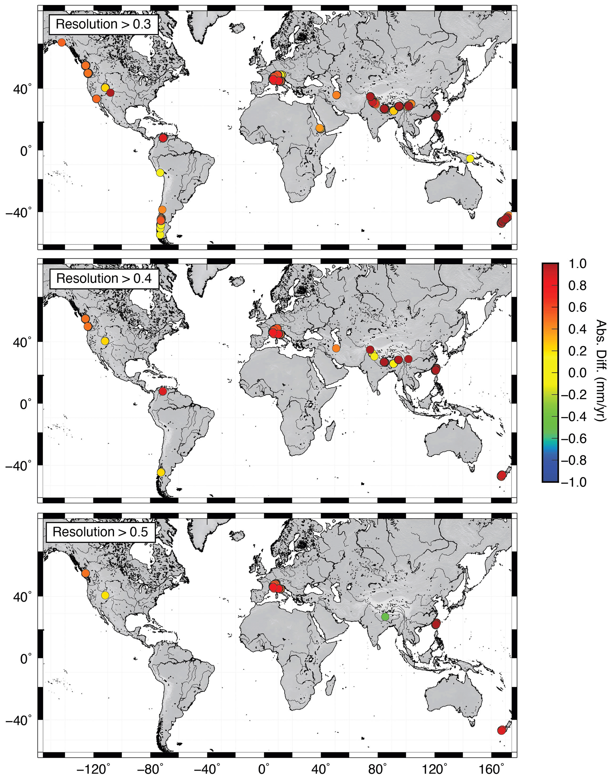
Figure 25Distribution of points where thermochonometric ages permit resolution of a change in erosion rate from 6 Ma to the present based on the inverse model analysis of Herman et al. (2013). Changes are expressed as a difference with distribution of values shown in Fig. 24. Each frame contains points above a specified resolution cut-off.
A better approach to that taken by Herman et al. (2013) or our analysis in Figs. 24 and 25 would be to assess resolution individually for each local data set. Because the number of data and data density vary from site to site, a constant value of the temporal resolution metric used as a threshold does not result in constant confidence in the erosion rate estimate, and the uniform resolution cut-off used by Herman et al. (2013) is not the best approach. An individual site assessment using the various metrics for resolution, including sensitivity to the prior model, data residuals and age maps as we have shown in this paper, would yield a more consistent level of confidence in local estimates. It is essential that such local site assessment be guided by recognition of the source of errors, as we have identified in Sect. 4 above. Otherwise, errors of unknown origin could be misidentified, for example as spatial averaging.
A change in the resolution analysis would not change the conclusions of Herman et al. (2013). The best-resolved parts of the models are the ones with multiple thermochronometers or elevation gradients, and it is these that serve as the basis for the signal of increasing erosion rate. Herman et al. (2013) did check for sensitivity to the prior (see the Supplement to their paper) and took into account data distributions and multiple posterior metrics, so the interpretation is fundamentally sound, and we see no reason to alter the conclusions of the original paper. The primary advantage of an improved resolution analysis would be to obtain a better estimate of the areas affected by changing erosion rates.
There is one bias in the Herman et al. (2013) study that has not appeared in any of the critiques of the paper. Sites with high erosion rates will be more likely to have experienced a recent acceleration than deceleration; sites with low modern rates are more likely to have experienced a deceleration in the recent past, and because low-rate sites are removed from the analysis due to lower resolution and because erosion rates cannot be negative, this does create a bias in the analysis suite of Herman et al. (2018). For a given modern erosion rate, there is some probability as to what the erosion rate would be at any point in the past, i.e. at 2 Ma, and this probability will be skewed because of non-negativity and truncation of low rates. We believe this skewness will be small because tectonic-driven erosion rate changes are heavily damped by geomorphic processes and isostasy (Whipple and Meade, 2006), but we acknowledge there are few data and no systematic treatment of this problem. This is a bias in the median change, i.e. the mean or median of the distribution of Fig. 24, and if this distribution were closer to the zero median, we would have investigated it in Herman et al. (2013). However, this is no bias in the result at any individual site, and so it is not the main topic of the current paper.
6.5 Data requirements for resolving late Cenozoic changes in erosion rate
There are several lessons learned from this exercise with regards to the ability of thermochronometric data to resolve changes in erosion rate over the last 5 Ma as well as for the physical conditions that would optimize future experimental design and case studies to address this problem.
First, temporal resolution is key for resolving erosion histories from thermochronometer data. To resolve a change in erosion rate in time requires a minimum of two ages with different depths to closure, requiring a distribution in elevation or differences in closure temperature. To resolve a Plio-Pleistocene change requires at least two ages of less than 5 Ma. Although high-relief profiles can provide good time records using a single chronometer, it is primarily through the use of multiple chronometers that an exhumation history with a change in rate can be resolved. Current low-temperature dating methods are limited to fission track dating and dating of apatite and zircon, but the range of sampled temperature can be expanded through the use of track length measurements or the use of grain size, composition or crystal damage diffusion models (Flowers et al., 2009). New methods incorporating models of helium diffusion profiles in apatite (e.g. thermochronometry, Shuster and Farley, 2004) or new ultra-low-temperature methods (e.g. OSL thermochronometry, King et al., 2016) will also greatly improve the ability to resolve young histories.
Second, the absolute value of the exhumation rate is important for resolving an erosion history. Because current methods have a limited range of closure temperature, to obtain ages under 5 Ma requires high rates of exhumation. High geothermal gradients also result in lower ages, but the range of values of heat flow is small compared to the potential range of values of exhumation rate. Obtaining young ages restricts study to regions experiencing rates of exhumation over about 0.1 mm yr−1.
Third, the need for high rates of exhumation necessarily pushes studies of exhumation rates into tectonically active areas, where the high relief and high rock uplift rates result in sufficiently high rates of exhumation. Tectonic activity does not preclude the resolution of temporal changes in exhumation rate. If there are spatial variations in exhumation rate, the number of data required to resolve both spatial and temporal variability increases, but there is no reason to presume that an analysis will fail to distinguish between spatial and temporal variability. It is important that temporal sampling does not inadvertently covary with spatial variability, for example by collecting higher-temperature thermochronometers from one region and lower-temperature chronometers from another region with differing exhumation histories. Provided that age–elevation profiles are obtained over a small area or multiple thermochronometers are available from a common location, temporal and spatial variability can be resolved.
Finally, there is no escape from the chicken-and-egg problem for identifying the underlying cause of variable erosion rates. Tectonic changes that drive a change in erosion rate or conversely erosion rate changes driving a change in tectonic uplift rate through isostasy cannot be distinguished. The best one can do is make a circumstantial case based on spatial limitations. For example, if an increase in erosion rate is observed with a geometric relationship with faults with independently determined activity and such a rate change is not observed in neighbouring regions, that provides circumstantial evidence that tectonics is changing independently of climate. However, it is important that there be a control case, i.e. a neighbouring region with no change in rate. Without a control, a single site cannot be used to argue cause and effect.
An extensive error analysis of the thermochronometric age inversion method of Herman et al. (2013) (GLIDE) yielded a number of conclusions, many of which are relevant to other studies based on thermal modelling of thermochronometric ages for cooling or exhumation histories. We summarize as follows.
-
The only significant model errors in GLIDE are associated with the calculation of the geotherm, demonstrating the importance of calibration against modern heat flow measurements or past P-T-t constraints and inclusion of appropriate physical boundary conditions. The importance of an accurate thermal model should not be underestimated.
-
Resolution errors are present in all thermochronometric age inversions but vary from effectively 0 with high data coverage to very important with sparse data. Temporal coverage, i.e. a wide range of ages with different closure temperatures or elevations, is much more important for constraining resolution than spatial distribution. At low resolution, solutions tend towards the prior value specified in the inversion unless there are older ages present that constrain the long-term erosion rate.
-
Posterior error metrics including resolution and posterior variance provide an accurate measure of resolution errors. Other valuable tests for resolution include sensitivity to the prior and analysis of data residuals. Metrics are relative, not absolute, measures. Posterior metrics do not accurately reflect model (e.g. geotherm) errors.
-
The spatial correlation bias hypothesized in Schildgen et al. (2018) does not exist in any significant way. There is spatial smoothing of exhumation estimates across discontinuities, but even these vanish with sufficient data. Gradients in exhumation rate resulted in no spatial averaging errors.
-
It is possible to obtain errors with false increases in erosion rate as resolution errors, but only for specific combinations of ages and the prior model. As resolution errors, they are characterized by bias to the prior, not spatial averaging, and are recognizable through the resolution statistics and sensitivity to the prior.
-
The basis for the conclusions of the Schildgen et al. (2018) paper was a combination of incorrect calculation of the ages used in their test models, post-processing of GLIDE inversion results using a biased operator, and a set of subjective interpretations, hypothesized but untested.
-
The original conclusions of Herman et al. (2013) remain largely valid. The interpretation as to the underlying cause as tectonic or climate change is, as it was in the original publication, open. The question as to the adequacy of the sample size to characterize global changes also remains open. The adequacy of the data to resolve changes at specific sites remains open to further assessment. However, we find no evidence for a bias in the analysis method, no systematic errors in the analysis method, or any reason to disregard the conclusions of that study.
As a second test for a spatial correlation bias towards false acceleration, we investigate the case of a constant gradient in exhumation rate. We set up a test data set based on a constant gradient varying from 0.1 to 1.0 mm yr−1 across a 90 km domain. There is no variation in the north–south direction, so the test case is effectively 1D, although we will show results in the form of 2D maps to be consistent with the other examples. We apply a regular grid of sample points across the domain, where we calculate ages from four thermochronometers. There is no elevation variation across the domain, so time resolution is determined exclusively from the closure temperatures of the various thermochronometers. Compared to the synthetic data models with the fault in the main paper, this model is simpler and more structured, thus making it simpler to identify sources of error and direct data–parameter relationships.
The erosion rate function and the synthetic ages are shown in Fig. A1. There are no ages under 2 Ma but many ages between 2 and 4 Ma, including some just over 2 Ma, which provides good resolution of both of the last two time steps.
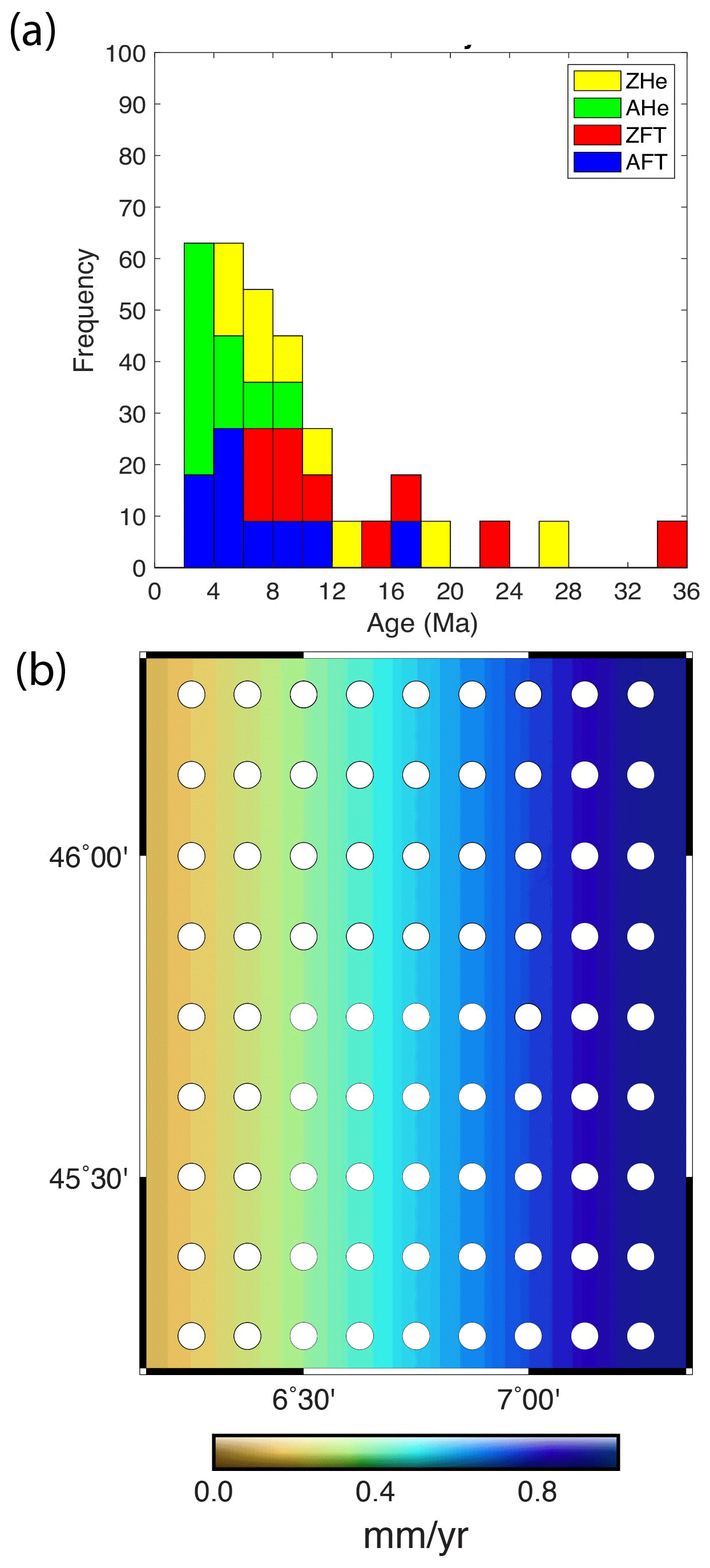
Figure A1(a) Synthetic age data and (b) age locations with the applied erosion rate field. Erosion rate has a constant gradient increasing from 0.1 mm yr−1 on the western edge to 1.0 on the eastern edge of the region. Ages are generated for four thermochronometric systems at each spatial point: apatite , apatite fission track, zircon , and zircon fission track methods.
Inversion of all data using GLIDE with a 30 km correlation length is shown in Fig. A2. We conducted two inversions, one with a prior erosion rate of 0.35 mm yr−1 and one with a prior erosion rate of 1.0 mm yr−1. The model has a runtime of 30 Ma, but we show only the last five time steps in Fig. A2. The last three time steps of this model are shown in Fig. 12. The temporal resolution and the reduced variance do not depend on the prior erosion rate and so are shown only once. Figure A2 shows that the solution is recovered very well for the 6 to 0 Ma time intervals. There is no significant error in these three intervals. In the 10 to 6 Ma time intervals there is a significant error in the regions of high uplift rate, but only in the case of the low prior. The sensitivity to the prior indicates that this is a resolution error, occurring because of the lack of age control on the fast-uplifting area during early time steps.
We consider only a subset of the data in an inverse model shown in Fig. A3, where the input data include only the two apatite systems. The solution reflects the change in resolution. The last two time intervals (4 to 0 Ma) are accurately reproduced, but the earlier time steps, now lacking any age constraints in the high uplift region, have significant errors in the high uplift zone, which is unsampled at early times. These errors are not present for the high prior model, indicating that these are resolution errors.
Figure A4 shows an inversion of only the zircon thermochronometric data. With older, high-temperature ages, the young time steps are poorly resolved but in spite of this are accurately estimated. This reflects the integral nature of the thermochronometric ages; an old age constrains the mean exhumation rate over its history, so for a case like this with a steady exhumation rate, the older ages provide an accurate estimate. The low resolution of the younger time steps reflects the lack of information regarding change over this time interval, so if there would be changes over the last two or three time steps, these would not be resolved. However, there is no sensitivity to the prior for these time steps because of the constraint provided by the old ages.
As a final test, we increased the correlation length from 30 to 100 km to try to increase spatial averaging and induce a spatial correlation bias (Fig. A5). There was essentially no effect.
We conducted an additional test of the Alpine Data Set E using a prior model equal to the true model (Fig. A6). As in all other cases, the parameters are recovered almost perfectly.
We conducted an experiment on the data from the Nanga Parbat region of the Himalaya to investigate whether or not data external to the massif had an inappropriate influence on the erosion rate inversion (Fig. A7). On the left of the figure is a model using all the data from the region. On the right is an inversion of only the data from the syntaxis core. Solutions within the core are essentially identical.
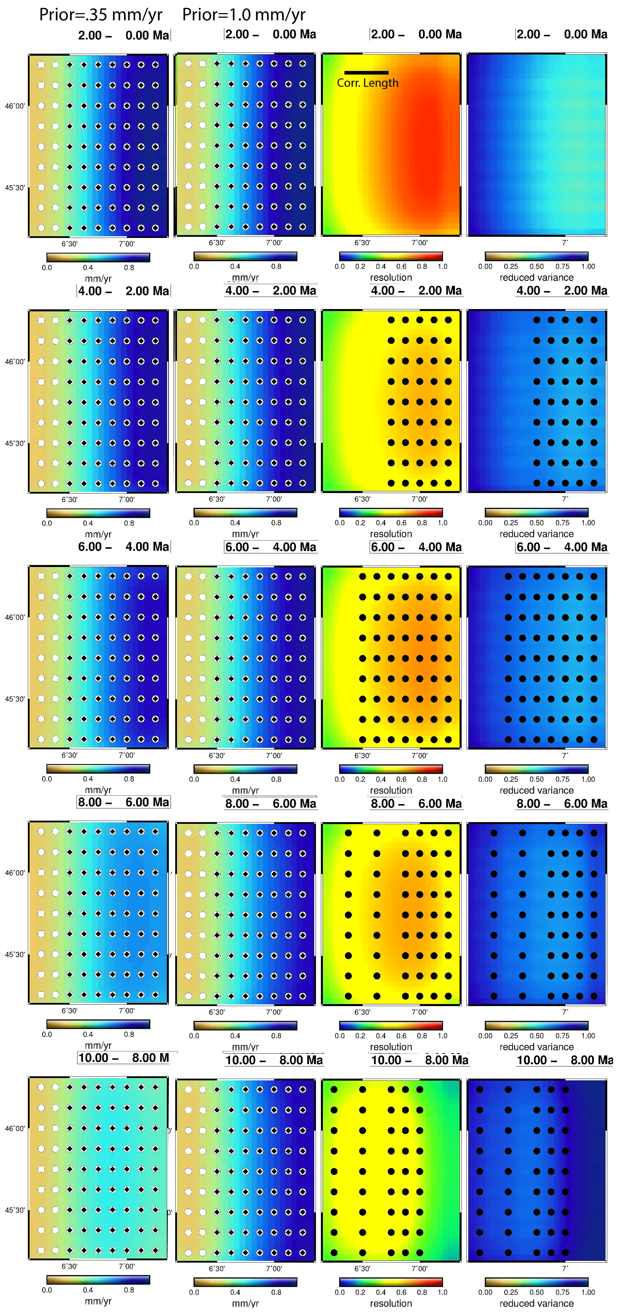
Figure A2GLIDE inversion of data including all four thermochronometric age systems. Each spatial point in the left column maps has four ages. Two inversions were run using a prior erosion rate of 0.35 mm yr−1 (left column) and a prior erosion rate of 1.0 mm yr−1 (second column). Resolution and reduced variance do not depend on the prior and are shown in the third and fourth columns, respectively. Ages that fall within the respective time interval are shown in the resolution and variance plots. The true solution is shown in Fig. A1.
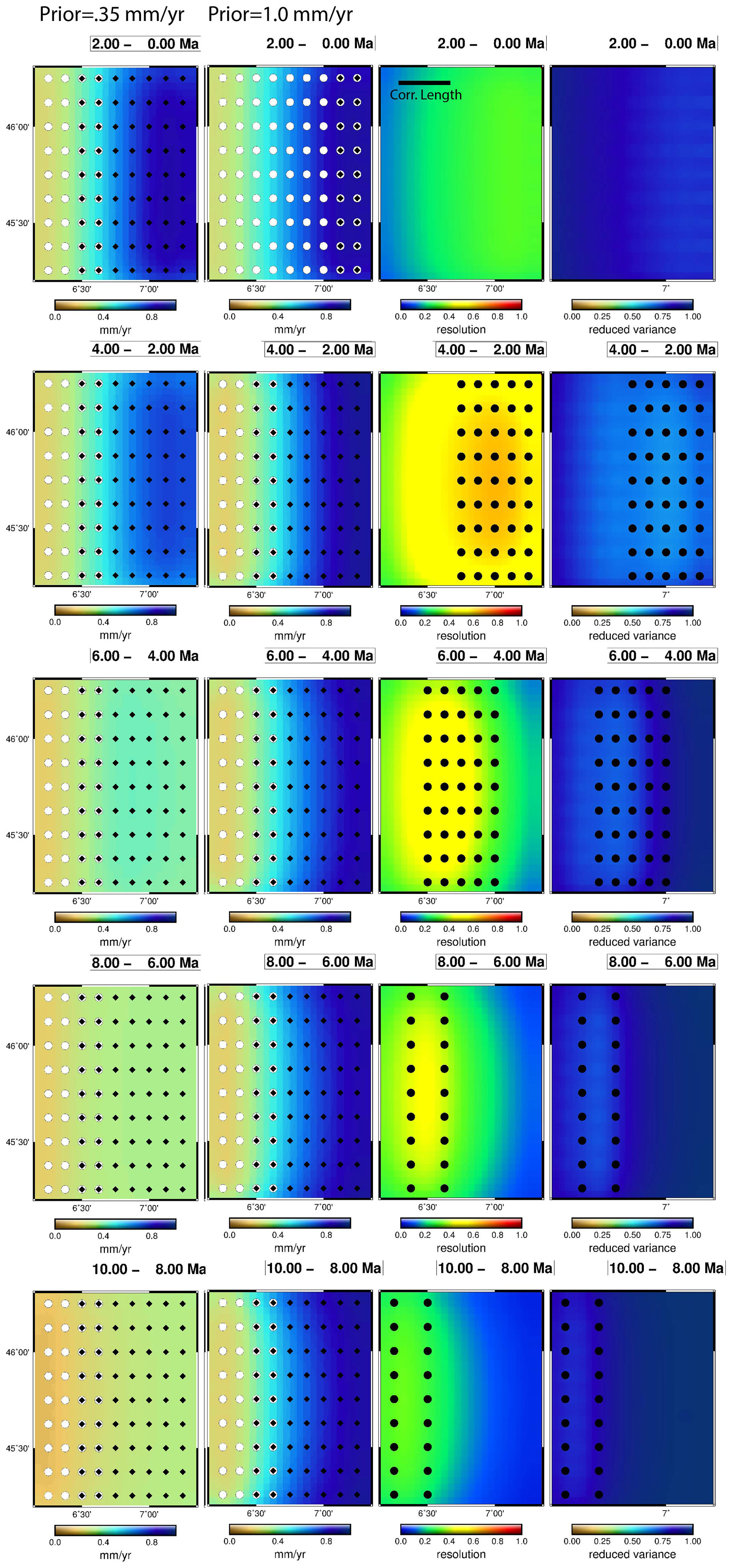
Figure A3GLIDE inversion of data including only the two apatite thermochronometric age systems. Each spatial point in the left column maps thus has two ages. Two inversions were run using a prior erosion rate of 0.35 mm yr−1 (left column) and a prior erosion rate of 1.0 mm yr−1 (second column). Resolution and reduced variance do not depend on the prior and are shown in the third and fourth columns, respectively. Ages that fall within the respective time interval are shown in the resolution and variance plots. The true solution is shown in Fig. A1.
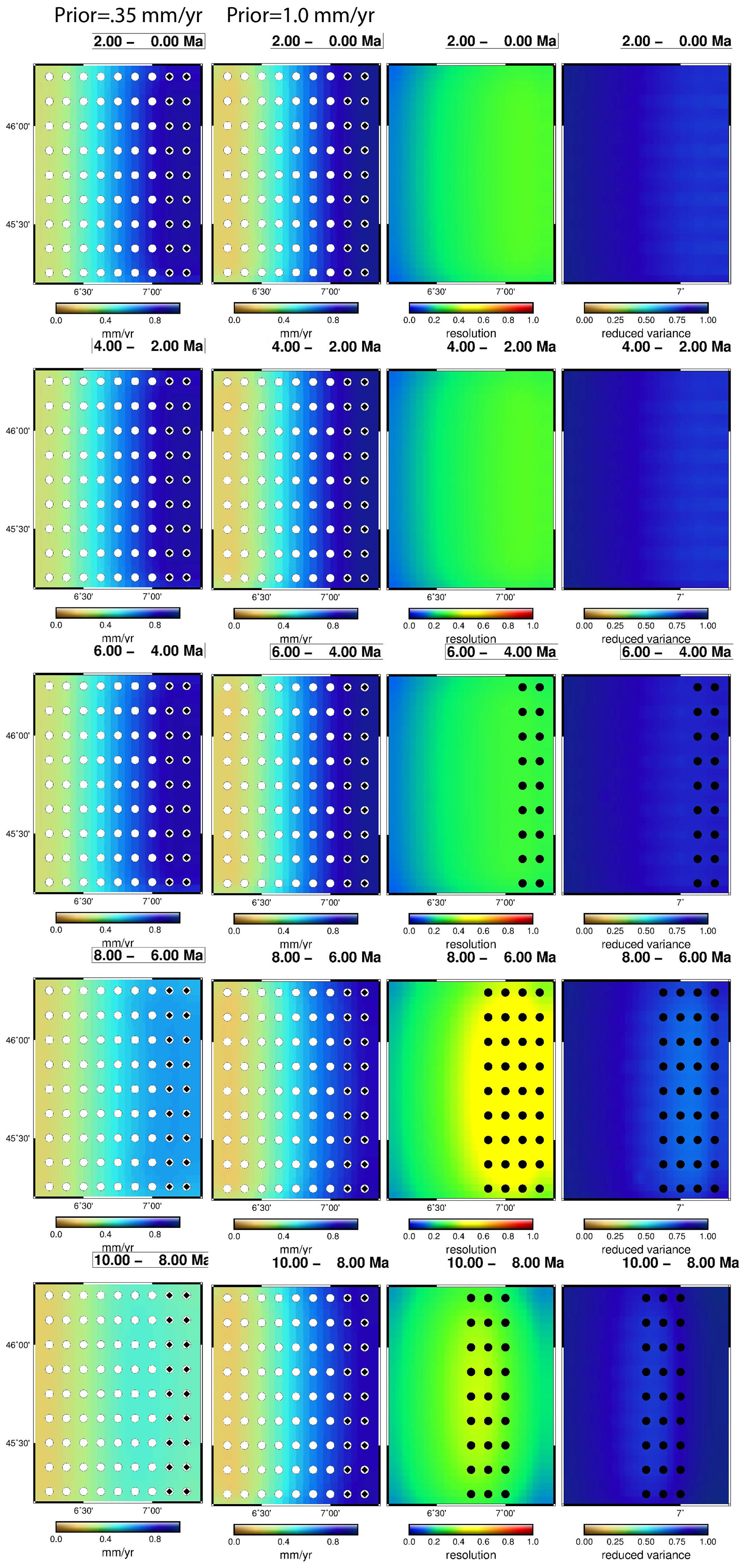
Figure A4GLIDE inversion of data including only the two zircon thermochronometric age systems. Each spatial point in the left column maps thus has two ages. Two inversions were run using a prior erosion rate of 0.35 mm yr−1 (left column) and a prior erosion rate of 1.0 mm yr−1 (second column). Resolution and reduced variance do not depend on the prior and are shown in the third and fourth columns, respectively. Ages that fall within the respective time interval are shown in the resolution and variance plots. The true solution is shown in Fig. A1.
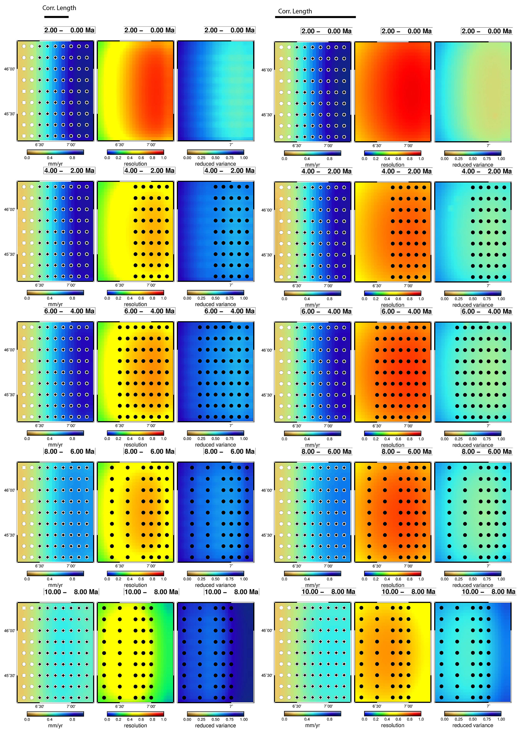
Figure A5GLIDE inversion of data including all four thermochronometric age systems. Two inversions were run using a correlation length scale of 30 km (left) and 100 km (right). Both runs use a prior erosion rate of 0.35 mm yr−1. Resolution and reduced variance are shown in the second and third columns for each model, respectively. Ages that fall within the respective time interval are shown in the resolution and variance plots. The true solution is shown in Fig. A1.
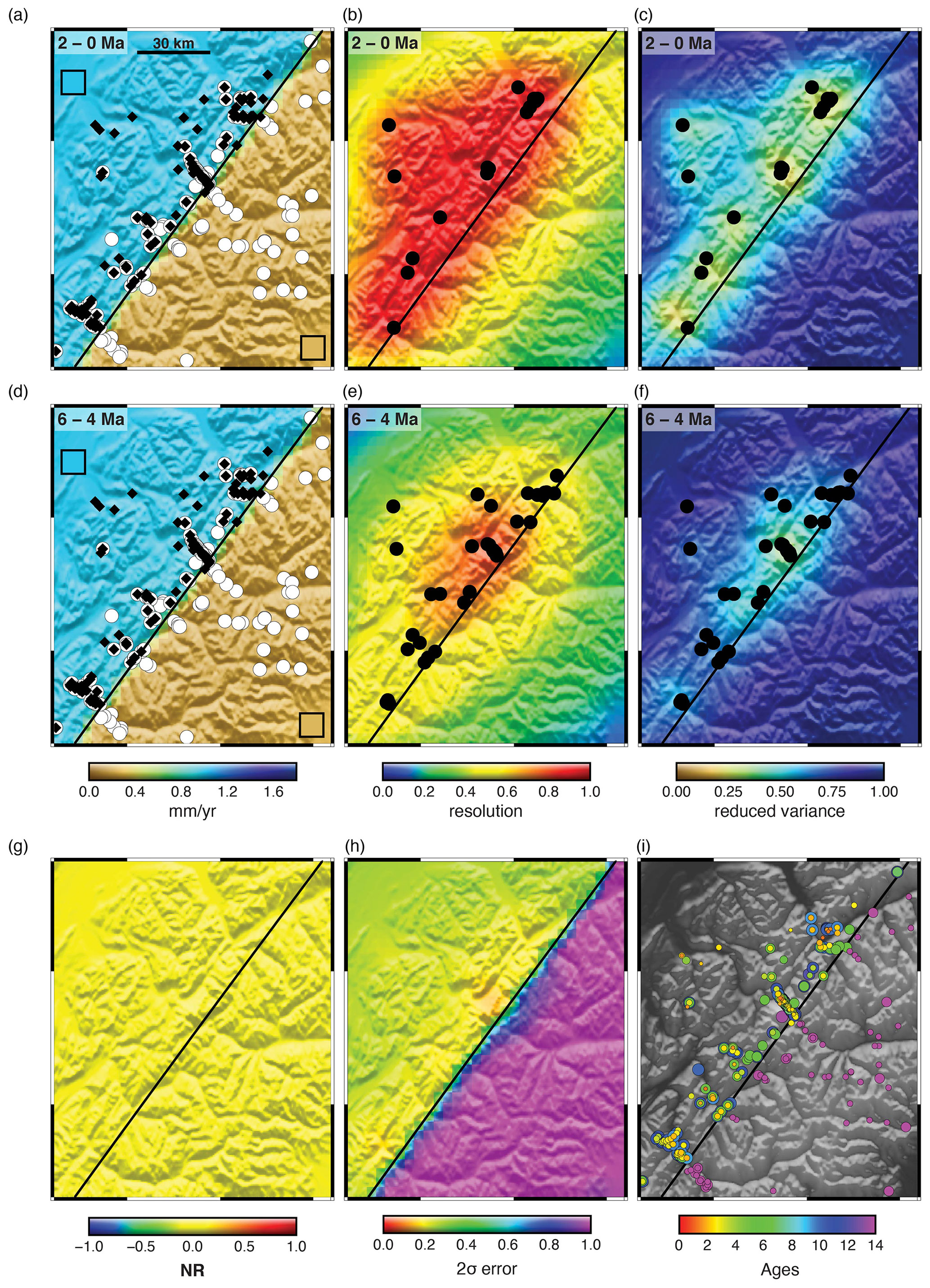
Figure A6Synthetic data inversion test using synthetic Data Set E calculated using the full, transient thermal model internal to GLIDE (Fig. 5). Prior erosion rates of 1.0 mm yr−1 in the north-western corner and 0.25 mm yr−1 in the south-eastern corner are used. This is equivalent to the true erosion rate used to generate the synthetic ages. Other inversion parameters in Table 1. See the Fig. 6 caption for other formatting details.
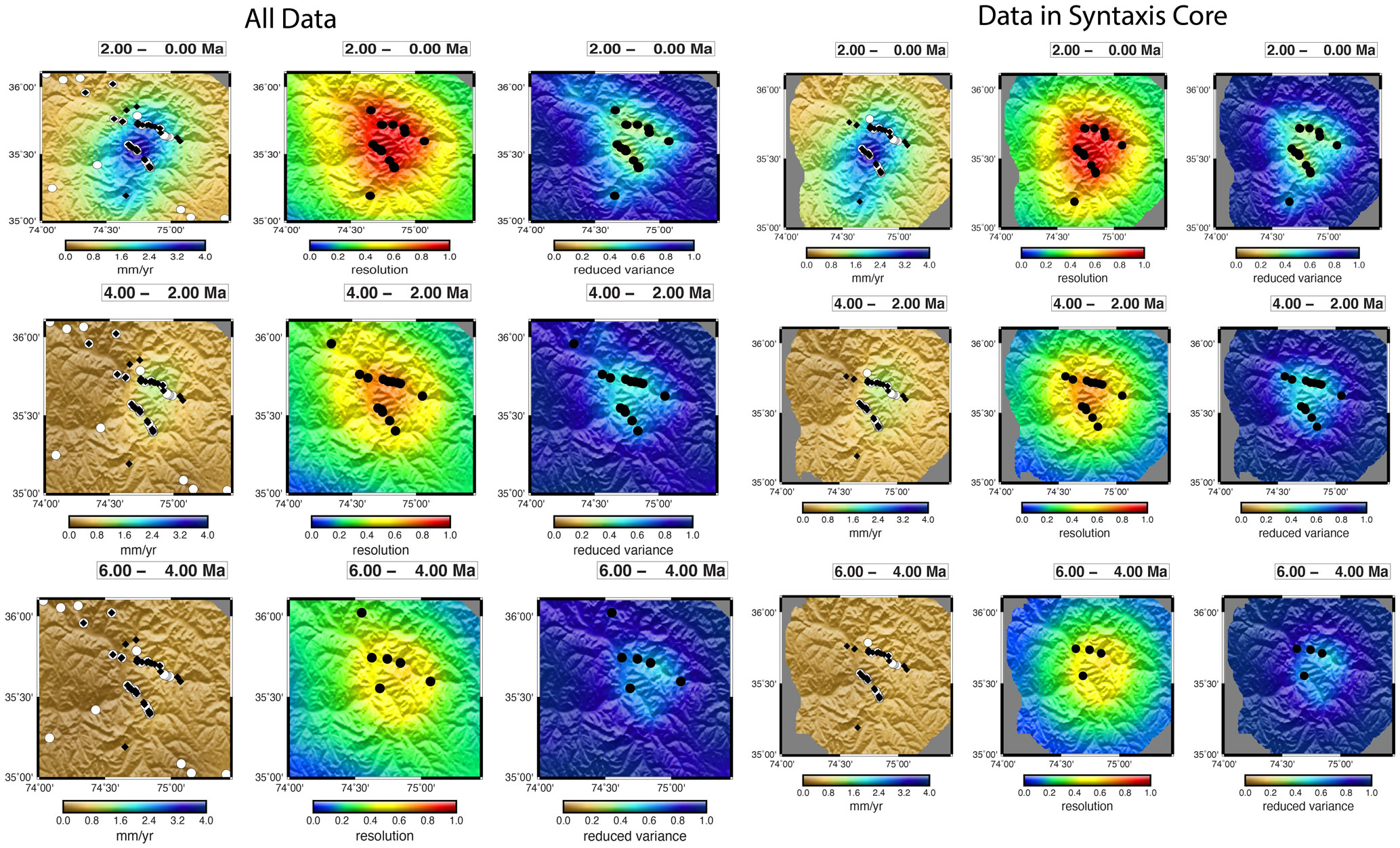
Figure A7Erosion rate history for the western Himalayan syntaxis in the region of Nanga Parbat using all data from Herman et al. (2013) and a second model using only ages from within the massif as defined by the Main Mantle Fault. Inferred erosion rates for three time intervals, from 6 Ma to present, are shown along with the temporal resolution and reduced variance. Erosion rate plots include ages less than 6 Ma as black diamonds and ages greater than 6 Ma as white dots. Resolution and variance plots include the ages that fall within the respective time interval. Note that there is essentially no difference in the solutions.
All codes including input files used for the modelling are available at https://doi.org/10.5281/zenodo.3992784 (cirederf13, 2020).
The research project and paper were conceived by SDW and FH. GLIDE code including resolution and error tracking was developed and written by FH, MF and RJ. Natural examples were modelled and researched by NS, TE and RY. Error analysis was developed by SDW and FH. Models were constructed and executed by FH and NS. The paper was written by SDW and FH, with contributions from TE, NS and MF.
Publisher's note: Copernicus Publications remains neutral with regard to jurisdictional claims in published maps and institutional affiliations.
This paper was edited by Richard Gloaguen and reviewed by four anonymous referees.
Antonelli, A., Kissling, W. D., Flantua, S. G., Bermúdez, M. A., Mulch, A., Muellner-Riehl, A. N., Kreft, H., Linder, H. P., Badgley, C., Fjeldså, J., Fritz, S. A., Rahbek, C., Herman, F., Hoogiemstra, H., and Hoorn, C.: Geological and climatic influences on mountain biodiversity, Nat. Geosci., 11, 718–725, 2018.
Armstrong, P. A., Ehlers, T. A., Chapman, D. S., Farley, K. A., and Kamp, P. J.: Exhumation of the central Wasatch Mountains, Utah: 1. Patterns and timing of exhumation deduced from low-temperature thermochronology data, J. Geophys. Res.-Sol. Ea., 108, https://doi.org/10.1029/2001JB001708, 2003.
Avdeev, B. and Niemi, N. A.: Rapid Pliocene exhumation of the central Greater Caucasus constrained by low-temperature thermochronometry Tectonics, 30, https://doi.org/10.1029/2010TC002808, 2011.
Backus, G. and Gilbert, F.: The resolving power of gross earth data, Geophys. J. Int., 16, 169–205, 1968.
Ballato, P., Landgraf, A., Schildgen, T. F., Stockli, D. F., Fox, M., Ghassemi, M. R., Kirby, E., and Strecker, M. R.: The growth of a mountain belt forced by base-level fall: Tectonics and surface processes during the evolution of the Alborz Mountains, N Iran, Earth Planet. Sc. Lett., 425, 204–218, 2015.
Barnes, J. B., Ehlers, T. A., Insel, N., McQuarrie, N., and Poulsen, C. J.: Linking orography, climate, and exhumation across the central Andes, Geology, 40, 1135–1138, 2012.
Batt, G. E. and Braun, J.: On the thermomechanical evolution of compressional orogens, Geophys. J. Int., 128, 364–382, 1997.
Batt, G. E., Braun, J., Kohn, B. P., and McDougall, I.: Thermochronological analysis of the dynamics of the Southern Alps, New Zealand, Geol. Soc. Am. Bull., 112, 250–266, 2000.
Batt, G. E., Brandon, M. T., Farley, K. A., and Roden-Tice, M.: Tectonic synthesis of the Olympic Mountains segment of the Cascadia wedge, using two-dimensional thermal and kinematic modeling of thermochronological ages, J. Geophys. Res.-Solid, 106, 26731–26746, 2001.
Beaumont, C., Kamp, P., Hamilton, J., and Fullsack, P.: The continental collision zone, South Island, New Zealand: Comparison of geodynamical models and observations, J. Geophys. Res.-Solid, 101, 3333–3359, 1996.
Becker, A.: The Jura Mountains: an active foreland Fold- and-Thrust belt?, Tectonophysics, 321, 381–406, 2000.
Bendick, R. and Ehlers, T. A.: Extreme localized exhumation at syntaxes initiated by subduction geometry, Geophys. Res. Lett., 41, 5861–5867, https://doi.org/10.1002/2014GL061026, 2014.
Berger, A. L. and Spotila, J. A.: Denudation and deformation in a glaciated orogenic wedge: The St. Elias orogen, Alaska, Geology, 36, 523–526, https://doi.org/10.1130/g24883a.1, 2008.
Berger, A. L., Gulick, S. P., Spotila, J. A., Upton, P., Jaeger, J. M., Chapman, J. B., Worthington, L. A., Pavlis, T. L., Ridgway, K. D., Willems, B. A., and McAleer, R. J.: Quaternary tectonic response to intensified glacial erosion in an orogenic wedge, Nat. Geosci., 1, 793–799, 2008a.
Berger, A. L., Spotila, J. A., Chapman, J. B., Pavlis, T. L., Enkelmann, E., Ruppert, N. A., and Buscher, J. T.: Architecture, kinematics, and exhumation of a convergent orogenic wedge: A thermochronological investigation of tectonic–climatic interactions within the central St. Elias orogen, Alaska, Earth Planet. Sc. Lett., 270, 13–24, 2008b.
Bertrand, A., Rosenberg, C., Rabaute, A., Herman, F., and Fügenschuh, B.: Exhumation mechanisms of the Tauern Window (Eastern Alps) inferred from apatite and zircon fission track thermochronology, Tectonics, 36, 207–228, 2017.
Birch, F.: Flow of heat in the Front Range, Colorado, Geol. Soc. Am. Bull., 61, 567–630, 1950.
Boccaletti, M., Corti, G., and Martelli, L.: Recent and active tectonics of the external zone of the Northern Apennines (Italy), Int. J. Earth Sci., 100, 1331–1348, https://doi.org/10.1007/s00531-010-0545-y, 2010.
Bolliger, T., Engesser, B., and Weidmann, M.: Première découverte de mammifères pliocènes dans le Jura neuchâteois, Eclogae Geologicae Helvetiae, 86, 1031–1068, 1993.
Bracciali, L., Parrish, R. R., Najman, Y., Smye, A., Carter, A., and Wijbrans, J. R.: Plio-Pleistocene exhumation of the eastern Himalayan syntaxis and its domal `pop-up', Earth-Sci. Rev., 160, 350–385, 2016.
Brandon, M. T., Roden-Tice, M. K., and Garver, J. I.: Late Cenozoic exhumation of the Cascadia accretionary wedge in the Olympic Mountains, northwest Washington State, Geol. Soc. Am. Bull., 110, 985–1009, 1998.
Braun, J.: Quantifying the effect of recent relief changes on age–elevation relationships, Earth Planet. Sc. Lett., 200, 331–343, 2002a.
Braun, J.: Estimating exhumation rate and relief evolution by spectral analysis of age–elevation datasets, Terra Nova, 14, 210–214, 2002b.
Braun, J.: Pecube: A new finite-element code to solve the 3D heat transport equation including the effects of a time-varying, finite amplitude surface topography, Comput. Geosci., 29, 787–794, 2003.
Braun, J., van der Beek, P., and Batt, G.: Quantitative thermochronology: numerical methods for the interpretation of thermochronological data, Cambridge University Press, Cambridge, 2006.
Braun, J., van Der Beek, P., Valla, P., Robert, X., Herman, F., Glotzbach, C., Pedersen, V., Perry, C., Simon-Labric, T., and Prigent, C.: Quantifying rates of landscape evolution and tectonic processes by thermochronology and numerical modeling of crustal heat transport using PECUBE, Tectonophysics, 524, 1–28, 2012.
Burbank, D. W., Blythe, A. E., Putkonen, J., Pratt-Sitaula, B., Gabet, E., Oskin, M., Barros, A., and Ojha, T. P.: Decoupling of erosion and precipitation in the Himalayas, Nature, 426, 652–655, 2003.
Campani, M., Herman, F., and Mancktelow, N.: Two-and three-dimensional thermal modeling of a low-angle detachment: Exhumation history of the Simplon Fault Zone, central Alps, J. Geophys. Res.-Sol. Ea., 115, https://doi.org/10.1029/2009JB007036, 2010.
Champagnac, J. D., Molnar, P., Anderson, R. S., Sue, C., and Delacou, B.: Quaternary erosion-induced isostatic rebound in the western Alps, Geology, 35, 195–198, 2007.
Champagnac, J. D., Schlunegger, F., Norton, K., von Blanckenburg, F., Abbühl, L. M., and Schwab, M.: Erosion-driven uplift of the modern Central Alps, Tectonophysics, 474, 236–249, 2009.
cirederf13: cirederf13/glide: GLIDE (glide), Zenodo [code], https://doi.org/10.5281/zenodo.3992784, 2020.
Coutand, I., Whipp Jr., D. M., Grujic, D., Bernet, M., Fellin, M. G., Bookhagen, B., Landry, K. R., Ghalley, S. K., and Duncan, C.: Geometry and kinematics of the Main Himalayan Thrust and Neogene crustal exhumation in the Bhutanese Himalaya derived from inversion of multithermochronologic data, J. Geophys. Res.-Solid, 119, 1446–1481, 2014.
Dahlen, F. A. and Barr, T. D.: Brittle frictional mountain building: 1. Deformation and mechanical energy budget, J. Geophys. Res.-Sol. Ea., 94, 3906–3922, https://doi.org/10.1029/JB094iB04p03906, 1989.
Dodson, M. H.: Closure temperature in cooling geochronological and petrological systems, Contrib. Mineral. Petrol., 40, 259–274, 1973.
Dodson, M. H. and McClelland-Brown, E.: Isotopic and palaeomagnetic evidence for rates of cooling, uplift and erosion, in: Geological Society Memoir, Geological Society of London, London, 315–325, 1985.
Egli, D. and Mancktelow, N.: The structural history of the Mont Blanc massif with regard to models for its recent exhumation, Swiss J. Geosci., 106, 469–489, 2013.
Ehlers, T. A.: Crustal thermal processes and the interpretation of thermochronometer data, Rev. Mineral. Geochem., 58, 315–350, 2005.
Ehlers, T. A. and Farley, K. A.: Apatite thermochronometry: methods and applications to problems in tectonic and surface processes, Earth Planet. Sc. Lett., 206, 1–14, 2003.
Ehlers, T. A., Armstrong, P. A., and Chapman, D. S.: Normal fault thermal regimes and the interpretation of low-temperature thermochronometers, Phys. Earth Planet. Int., 126, 179–194, https://doi.org/10.1016/S0031-9201(01)00254-0, 2001.
Ehlers, T. A., Willett, S. D., Armstrong, P. A., and Chapman, D. S.: Exhumation of the central Wasatch Mountains, Utah: 2. Thermokinematic model of exhumation, erosion, and thermochronometer interpretation, J. Geophys. Res.-Solid, 108, https://doi.org/10.1029/2001JB001723, 2003.
Ehlers, T. A., Farley, K. A., Rusmore, M. E., and Woodsworth, G. J.: Apatite (U-Th)/He signal of large-magnitude accelerated glacial erosion, southwest British Columbia, Geology, 34, 765–768, https://doi.org/10.1130/022507.1, 2006.
England, P. and Molnar, P.: Surface uplift, uplift of rocks, and exhumation of rocks, Geology, 18, 1173–1177, https://doi.org/10.1130/0091-7613(1990)018<1173:SUUORA>2.3.CO;2, 1990.
England, P. C. and Thompson, A. B.: Pressure – temperature – time paths of regional metamorphism I. heat transfer during the evolution of regions of thickened continental crust, J. Petrol., 25, 894–928, https://doi.org/10.1093/petrology/25.4.894, 1984.
Fantoni, R., Massari, F., Minervini, M., Rogledi, S., and Rossi, M.: Il Messiniano del margine Sudalpino-Padano: relazioni tra contesto strutturale e stratigrafico-deposizionale, Geologica Insubrica, 6, 95–108, 2001.
Farley, K. A., Rusmore, M. E., and Bogue, S. W.: Post-10 Ma uplift and exhumation of the northern Coast Mountains, British Columbia, Geology, 29, 99–102, 2001.
Fellin, M. G., Chen, C. Y., Willett, S. D., Christl, M., and Chen, Y. G.: Erosion rates across space and timescales from a multi-proxy study of rivers of eastern Taiwan, Global Planet. Change, 157, 174–193, 2017.
Fitzgerald, P. G. and Gleadow, A. J.: Fission-track geochronology, tectonics and structure of the Transantarctic Mountains in northern Victoria Land, Antarctica, Chem. Geol., 73, 169–198, 1988.
Fitzgerald, P. G., Sorkhabi, R. B., Redfield, T. F., and Stump, E.: Uplift and denudation of the central Alaska Range: A case study in the use of apatite fission track thermochronology to determine absolute uplift parameters, J. Geophys. Res.-Solid, 100, 20175–20191, 1995.
Flowers, R. M., Ketcham, R. A., Shuster, D. L., and Farley, K. A.: Apatite (U–Th) He thermochronometry using a radiation damage accumulation and annealing model, Geochim. Cosmochim. Ac., 73, 2347–2365, https://doi.org/10.1016/j.gca.2009.01.015, 2009.
Fox, M., Herman, F., Willett, S. D., and May, D. A.: A linear inversion method to infer exhumation rates in space and time from thermochronometric data, Earth Surf. Dynam., 2, 47–65, https://doi.org/10.5194/esurf-2-47-2014, 2014.
Fox, M., Herman, F., Kissling, E., and Willett, S. D.: Rapid exhumation in the Western Alps driven by slab detachment and glacial erosion, Geology, 43, 379–382, 2015.
Fox, M., Herman, F., Willett, S. D., and Schmid, S. M.: The exhumation history of the European Alps inferred from linear inversion of thermochronometric data, Am. J. Sci., 316, 505–541, 2016.
Franklin, J. N.: Well-posed stochastic extensions of ill-posed linear problems, J. Math. Anal. Appl., 31, 682–716, 1970.
Fuller, C. W., Willett, S. D., Fisher, D., and Lu, C. Y.: A thermomechanical wedge model of Taiwan constrained by fission-track thermochronometry, Tectonophysics, 425, 1–24, 2006.
Furlong, K. P. and Chapman, D. S.: Heat Flow, Heat Generation, and the Thermal State of the Lithosphere, Annu. Rev. Earth Planet. Sci., 41, 385–410, https://doi.org/10.1146/annurev.earth.031208.100051, 2013.
Gallagher, K.: Transdimensional inverse thermal history modeling for quantitative thermochronology, J. Geophys. Res.-Solid, 117, https://doi.org/10.1029/2011JB008825, 2012.
Glotzbach, C., Van Der Beek, P. A., and Spiegel, C.: Episodic exhumation and relief growth in the Mont Blanc massif, Western Alps from numerical modelling of thermochronology data, Earth Planet. Sc. Lett., 304, 417–430, 2011.
Grasemann, B. and Mancktelow, N. S.: Two-dimensional thermal modelling of normal faulting: the Simplon Fault Zone, Central Alps, Switzerland, Tectonophysics, 225, 155–165, 1993.
Harrison, T. M., Armstrong, R. L., Naeser, C., and Harakal, J. E.: Geochronology and thermal history of the Coast Plutonic complex, near Prince Rupert, British Columbia, Can. J. Earth Sci., 16, 400–410, https://doi.org/10.1139/e79-038, 1979.
Harrison, T. M., Ryerson, F. J., Le Fort, P., Yin, A., Lovera, O. M., and Catlos, E. J.: A late Miocene-Pliocene origin for the central Himalayan inverted metamorphism, Earth Planet. Sc. Lett., 146, E1–E7, 1997.
Herman, F. and Brandon, M.: Mid-latitude glacial erosion hotspot related to equatorial shifts in southern Westerlies, Geology, 43, 987–990, 2015.
Herman, F., Cox, S. C., and Kamp, P. J.: Low-temperature thermochronology and thermokinematic modeling of deformation, exhumation, and development of topography in the central Southern Alps, New Zealand, Tectonics, 28, https://doi.org/10.1029/2008TC002367, 2009.
Herman, F., Copeland, P., Avouac, J. P., Bollinger, L., Mahéo, G., Le Fort, P., Rai, S., Foster, D., Pêcher, A., Stüwe, K., and Henry, P.: Exhumation, crustal deformation, and thermal structure of the Nepal Himalaya derived from the inversion of thermochronological and thermobarometric data and modeling of the topography, J. Geophys. Res.-Solid, 115, https://doi.org/10.1029/2008JB006126, 2010.
Herman, F., Seward, D., Valla, P. G., Carter, A., Kohn, B., Willett, S. D., and Ehlers, T. A.: Worldwide acceleration of mountain erosion under a cooling climate, Nature, 504, 423–426, 2013.
Hurford, A. J.: Cooling and uplift patterns in the Lepontine Alps South Central Switzerland and an age of vertical movement on the Insubric fault line, Contrib. Mineral. Petrol., 92, 413–427, 1986.
Jackson, D. D.: Most squares inversion, J. Geophys. Res., 81, 1027–1030, 1976.
Jackson, D. D.: The use of a priori data to resolve non-uniqueness in linear inversion, Geophys. J. Int., 57, 137–157, 1979.
Jiao, R., Herman, F., and Seward, D.: Late Cenozoic exhumation model of New Zealand: Impacts from tectonics and climate, Earth-Sci. Rev., 166, 286–298, 2017.
Ketcham, R. A.: Forward and inverse modeling of low-temperature thermochronometry data, Rev. Mineral. Geochem., 58, 275–314, 2005.
King, G. E., Guralnik, B., Valla, P. G., and Herman, F.: Trapped-charge thermochronometry and thermometry: A status review, Chem. Geol., 446, 3–17, https://doi.org/10.1016/j.chemgeo.2016.08.023, 2016.
Kirby, E.: Doubt cast on how the pace of global glacial erosion responds to climate cooling: Nature, 559, 34–35, https://doi.org/10.1038/d41586-018-05563-6, 2018.
Koptev, A., Ehlers, T. A., Nettesheim, M., and Whipp, D.: Response of a rheologically stratified lithosphere to subduction of an indenter-shaped plate: Insights into localized exhumation at orogen syntaxes, Tectonics, 1908–1930, https://doi.org/10.1029/2018TC005455, 2019.
Lawson, C. L. and Hanson, R. J.: Solving least squares problems, Prentice-Hall, Englewood Cliffs, NJ, 1974.
Lees, C. H.: On the shapes of the isogeotherms under mountain ranges in radio-active districts, P. Roy. Soc. Lond. A, 83, 339–346, 1910.
Legendre, A. M.: Nouvelles méthodes pour la détermination des orbites des comètes, F. Didot, Paris, 1805.
Lock, J. and Willett, S.: Low-temperature thermochronometric ages in fold-and-thrust belts, Tectonophysics, 456, 147–162, 2008.
Mancktelow, N. S. and Grasemann, B.: Time-dependent effects of heat advection and topography on cooling histories during erosion, Tectonophysics, 270, 167–195, 1997.
Margirier, A., Audin, L., Robert, X., Herman, F., Ganne, J., and Schwartz, S.: Time and mode of exhumation of the Cordillera Blanca batholith (Peruvian Andes), J. Geophys. Res.-Solid Earth, 121, 6235–6249, 2016.
Marsaglia, G.: Ratios of Normal Variables and Ratios of Sums of Uniform Variables, J. Am. Statist. Assoc., 60, 193–204, https://doi.org/10.1080/01621459.1965.10480783, 1965.
McKenzie, D.: Some remarks on the development of sedimentary basins, Earth Planet. Sc. Lett., 40, 25–32, https://doi.org/10.1016/0012-821X(78)90071-7, 1978.
McQuarrie, N. and Ehlers, T. A.: Influence of thrust belt geometry and shortening rate on thermochronometer cooling ages: Insights from thermokinematic and erosion modeling of the Bhutan Himalaya, Tectonics, 34, 1055–1079, 2015.
McQuarrie, N. and Ehlers, T. A.: Techniques for understanding fold-thrust belt kinematics and thermal evolution, in: Linkages and Feedbacks in Orogenic Process: A volume in Honor of Robert. D. Hatcher Jr., Geological Society of America, Boulder, CO, USA, Memoirs, 213, 25–54, 2017.
Menke, W.: Geophysical Data Analysis: Discrete Inverse Theory, Academic Press, Amsterdam, p. 330, ISBN 978-0-12-397160-9, 2012.
Michel, L., Ehlers, T. A., Glotzbach, C., Adams, B. A., and Stübner, K.: Tectonic and glacial contributions to focused exhumation in the Olympic Mountains, Washington, USA, Geology, 46, 491–494, 2018.
Michel, L., Glotzbach, C., Falkowski, S., Adams, B. A., and Ehlers, T. A.: How steady are steady-state mountain belts? A reexamination of the Olympic Mountains (Washington State, USA), Earth Surf. Dynam., 7, 275–299, https://doi.org/10.5194/esurf-7-275-2019, 2019.
Molnar, P.: The rise of mountain ranges and the evolution of humans: a causal relation?, Irish J. Earth Sci., 10, 199–207, 1990.
Molnar, P.: Late Cenozoic increase in accumulation rates of terrestrial sediment: How might climate change have affected erosion rates?, Annu. Rev. Earth Planet. Sci., 32, 67–89, 2004.
Molnar, P. and England, P.: Late Cenozoic uplift of mountain ranges and global climate change: chicken or egg?, Nature, 346, 29–34, 1990.
Moore, M. A. and England, P. C.: On the inference of denudation rates from cooling ages of minerals, Earth Planet. Sc. Lett., 185, 265–284, 2001.
Mutz, S. G. and Ehlers, T. A.: Detection and explanation of spatiotemporal patterns in Late Cenozoic palaeoclimate change relevant to Earth surface processes, Earth Surf. Dynam., 7, 663–679, https://doi.org/10.5194/esurf-7-663-2019, 2019.
Mutz, S. G., Ehlers, T. A., Werner, M., Lohmann, G., Stepanek, C., and Li, J.: Estimates of late Cenozoic climate change relevant to Earth surface processes in tectonically active orogens, Earth Surf. Dynam., 6, 271–301, https://doi.org/10.5194/esurf-6-271-2018, 2018.
Nettesheim, M., Ehlers, T. A., Whipp, D. M., and Koptev, A.: The influence of upper-plate advance and erosion on overriding plate deformation in orogen syntaxes, Solid Earth, 9, 1207–1224, https://doi.org/10.5194/se-9-1207-2018, 2018.
Ory, J. and Pratt, R. G.: Are our parameter estimators biased? The significance of finite-difference regularization operators, Inverse Probl., 11, 397–424, 1995.
Parrish, R.: Cenozoic Thermal Evolution and Tectonics of the Coast Mountains of British-Columbia, 1. Fission-Track Dating, Apparent Uplift Rates, and Patterns of Uplift, Tectonics, 2, 601–631, 1983.
Pazzaglia, F. J. and Brandon, M. T.: A fluvial record of long-term steady-state uplift and erosion across the Cascadia forearc high, western Washington State, Am. J. Sci., 301, 385–431, 2001.
Reiners, P., Ehlers, T., and Zeitler, P.: Past, present, and future of thermochronology: Low-Temperature Thermochronology: Techniques, Interpretations, And Applications, Rev. Miner. Geochem., 58, 1–18, https://doi.org/10.2138/rmg.2005.58.1, 2005.
Reiners, P. W. and Brandon, M. T.: Using thermochronology to understand orogenic erosion, Annu. Rev. Earth Planet. Sci., 34, 419–466, 2006.
Reiners, P. W., Ehlers, T. A., Mitchell, S. G., and Montgomery, D. R.: Coupled spatial variations in precipitation and long-term erosion rates across the Washington Cascades, Nature, 426, 645–647, 2003.
Schildgen, T. F., van der Beek, P. A., Sinclair, H. D., and Thiede, R. C.: Spatial correlation bias in late-Cenozoic erosion histories derived from thermochronology, Nature, 559, 89–93, 2018.
Sclater, J. G. and Francheteau, J.: The Implications of Terrestrial Heat Flow Observations on Current Tectonic and Geochemical Models of the Crust and Upper Mantle of the Earth, Geophys. J. Roy. Astron. Soc., 20, 509–542, https://doi.org/10.1111/j.1365-246X.1970.tb06089.x, 1970.
Seward, D. and Mancktelow, N. S.: Neogene kinematics of the central and western Alps: Evidence from fission-track dating, Geology, 22, 803–806, 1994.
Shuster, D. L. and Farley, K. A.: 4He/3He thermochronometry, Earth Planet. Sc. Lett., 217, 1–17, https://doi.org/10.1016/S0012-821X(03)00595-8, 2004.
Shuster, D. L., Ehlers, T. A., Rusmoren, M. E., and Farley, K. A.: Rapid glacial erosion at 1.8 Ma revealed by thermochronometry, Science, 310, 1668–1670, 2005.
Shuster, D. L., Cuffey, K. M., Sanders, J. W., and Balco, G.: Thermochronometry reveals headward propagation of erosion in an alpine landscape, Science, 332, 84–88, 2011.
Siravo, G., Faccenna, C., Gérault, M., Becker, T. W., Fellin, M. G., Herman, F., and Molin, P.: Slab flattening and the rise of the Eastern Cordillera, Colombia, Earth Planet. Sc. Lett., 512, 100–110, 2019.
Starke, J., Ehlers, T. A., and Schaller, M.: Tectonic and Climatic Controls on the Spatial Distribution of Denudation Rates in Northern Chile (18∘ S to 23∘ S) Determined from Cosmogenic Nuclides, J. Geophys. Res.-Earth, 122, 1949–1971, https://doi.org/10.1002/2016JF004153, 2017.
Stüwe, K. and Hintermüller, M.: Topography and isotherms revisited: the influence of laterally migrating drainage divides, Earth Planet. Sc. Lett., 184, 287–303, https://doi.org/10.1016/S0012-821X(00)00315-0, 2000.
Stüwe, K., White, L., and Brown, R.: The influence of eroding topography on steady-state isotherms. Application to fission track analysis Earth Planet. Sc. Lett., 124, 63–74, 1994.
Sutherland, R., Gurnis, M., Kamp, P. J., and House, M. A.: Regional exhumation history of brittle crust during subduction initiation, Fiordland, southwest New Zealand, and implications for thermochronologic sampling and analysis strategies, Geosphere, 5, 409–425, 2009.
Tarantola, A.: Inverse problem theory and methods for model parameter estimation, Society for Industrial and Applied Mathematics, 89, 2005.
Tarantola, A. and Valette, B.: Generalized nonlinear inverse problems solved using the least squares criterion, Rev. Geophys., 20, 219–232, 1982.
Thiede, R. C. and Ehlers, T. A.: Large spatial and temporal variations in Himalayan denudation, Earth Planet. Sc. Lett., 371, 278–293, 2013.
Thiede, R. C., Ehlers, T. A., Bookhagen, B., and Strecker, M. R.: Erosional variability along the northwest Himalaya, J. Geophys. Res.-Earth, 114, F01015, https://doi.org/10.1029/2008JF001010, 2009.
Thomson, S. N., Brandon, M. T., Tomkin, J. H., Reiners, P. W., Vásquez, C., and Wilson, N. J.: Glaciation as a destructive and constructive control on mountain building, Nature, 467, 313–317, 2010a.
Thomson, S. N., Brandon, M. T., Reiners, P. W., Zattin, M., Isaacson, P. J., and Balestrieri, M. L.: Thermochronologic evidence for orogen-parallel variability in wedge kinematics during extending convergent orogenesis of the northern Apennines, Italy, Bulletin, 122, 1160–1179, 2010b.
Tippett, J. M. and Kamp, P. J.: Fission track analysis of the late Cenozoic vertical kinematics of continental Pacific crust, South Island, New Zealand, J. Geophys. Res.-Solid, 98, 16119–16148, 1993.
Valla, P. G., Shuster, D. L., and Van Der Beek, P. A.: Significant increase in relief of the European Alps during mid-Pleistocene glaciations, Nat. Geosci., 4, 688–692, 2011.
Valla, P. G., van der Beek, P. A., Shuster, D. L., Braun, J., Herman, F., Tassan-Got, L., and Gautheron, C.: Late Neogene exhumation and relief development of the Aar and Aiguilles Rouges massifs (Swiss Alps) from low-temperature thermochronology modeling and thermochronometry, J. Geophys. Res.-Earth, 117, F01004, https://doi.org/10.1029/2011JF002043, 2012.
Vernon, A. J., Van Der Beek, P. A., Sinclair, H. D., and Rahn, M. K.: Increase in late Neogene denudation of the European Alps confirmed by analysis of a fission-track thermochronology database, Earth Planet. Sc. Lett., 270, 316–329, 2008.
Vincent, S. J., Somin, M. L., Carter, A., Vezzoli, G., Fox, M., and Vautravers, B.: Testing Models of Cenozoic Exhumation in the Western Greater Caucasus, Tectonics, 39, e2018TC005451, https://doi.org/10.1029/2018TC005451, 2020.
Wagner, G. A. and Reimer, G. M.: Fission track tectonics: the tectonic interpretation of fission track apatite ages, Earth Planet. Sc. Lett., 14, 263–268, 1972.
Wagner, G. A., Miller, D. S., and Jäger, E.: Fission track ages on apatite of Bergell rocks from central Alps and Bergell boulders in Oligocene sediments, Earth Planet. Sc. Lett., 45, 355–360, 1979.
Whipp Jr., D. M., Ehlers, T. A., Blythe, A. E., Huntington, K. W., Hodges, K. V., and Burbank, D. W.: Plio-Quaternary exhumation history of the central Nepalese Himalaya: 2. Thermokinematic and thermochronometer age prediction model, Tectonics, 26, https://doi.org/10.1029/2006TC001991, 2007.
Whipple, K. and Meade, B.: Orogen response to changes in climatic and tectonic forcing, Earth Planet. Sc. Lett., 243, 218–228, https://doi.org/10.1016/j.epsl.2005.12.022, 2006.
Willenbring, J. K. and Jerolmack, D. J.: The null hypothesis: globally steady rates of erosion, weathering fluxes and shelf sediment accumulation during Late Cenozoic mountain uplift and glaciation, Terra Nova, 28, 11–18, 2016.
Willett, S. D.: Orogeny and orography: The effects of erosion on the structure of mountain belts, J. Geophys. Res.-Solid, 104, 28957–28981, 1999.
Willett, S. D.: Late Neogene erosion of the Alps: A climate driver?, Annu. Rev. Earth Planet. Sci., 38, 411–437, 2010.
Willett, S. D. and Brandon, M. T.: On steady states in mountain belts, Geology, 30, 175–178, 2002.
Willett, S. D. and Brandon, M. T.: Some analytical methods for converting thermochronometric age to erosion rate, Geochem. Geophy. Geosy., 14, 209–222, 2013.
Willett, S. D., Fisher, D., Fuller, C., En-Chao, Y., and Chia-Yu, L.: Erosion rates and orogenic-wedge kinematics in Taiwan inferred from fission-track thermochronometry, Geology, 31, 945–948, 2003.
Willett, S. D., Schlunegger, F., and Picotti, V.: Messinian climate change and erosional destruction of the central European Alps, Geology, 34, 613–616, 2006.
Wobus, C. W., Hodges, K. V., and Whipple, K. X.: Has focused denudation sustained active thrusting at the Himalayan topographic front?, Geology, 31, 861–864, 2003.
Yang, R., Fellin, M. G., Herman, F., Willett, S. D., Wang, W., and Maden, C.: Spatial and temporal pattern of erosion in the Three Rivers Region, southeastern Tibet, Earth Planet. Sc. Lett., 433, 10–20, https://doi.org/10.1016/j.epsl.2015.10.032, 2016.
Zeitler, P.: Cooling History of the Nw Himalaya, Pakistan: Tectonics, 4, 127–151, 1985.
Zeitler, P. K., Johnson, N. M., Naeser, C. W., and Tahirkheli, R. A.: Fission-track evidence for Quaternary uplift of the Nanga Parbat region, Pakistan, Nature, 298, 255–257, 1982.
Zhang, P., Molnar, P., and Downs, W. R.: Increased sedimentation rates and grain sizes 2–4 Myr ago due to the influence of climate change on erosion rates, Nature, 410, 891–897, 2001.
- Abstract
- Introduction
- Bias and resolution in thermochronometry-derived exhumation rates
- GLIDE inversion method and error analysis
- Synthetic data tests for resolution and model errors
- Tectonics and spatial variability in thermochronometric ages
- Discussion
- Conclusions
- Appendix A: Additional synthetic data models
- Code and data availability
- Author contributions
- Disclaimer
- Review statement
- References