How do modeling choices and erosion zone locations impact the representation of connectivity and the dynamics of suspended sediments in a multi-source soil erosion model?

Soil erosion and suspended sediment transport understanding is an important issue in terms of soil and water resources management in the critical zone. In mesoscale watersheds (>10 km²) the spatial distribution of potential sediment sources within the catchment associated with rainfall dynamics is considered to be the main factor in the observed suspended sediment flux variability within and between runoff events. Given the high spatial heterogeneity that can exist for such scales of interest, distributed physically based models of soil erosion and sediment transport are powerful tools to distinguish the specific effect of structural and functional connectivity on suspended sediment flux dynamics. As the spatial discretization of a model and its parameterization can crucially influence how the structural connectivity of the catchment is represented in the model, this study analyzed the impact of modeling choices in terms of the contributing drainage area (CDA) threshold to define the river network and of Manning's roughness parameter (n) on the sediment flux variability at the outlet of two geomorphologically distinct watersheds. While the modeled liquid and solid discharges were found to be sensitive to these choices, the patterns of the modeled source contributions remained relatively similar when the CDA threshold was restricted to the range of 15 to 50 ha, with n restricted to the range 0.4–0.8 on the hillslopes and to 0.025–0.075 in the river. The comparison of the two catchments showed that the actual location of sediment sources was more important than the choices made during discretization and parameterization of the model. Among the various structural connectivity indicators used to describe the geological sources, the mean distance to the stream was the most relevant proxy for the temporal characteristics of the modeled sedigraphs.

1 Introduction

Soil erosion and suspended sediment transport are natural processes that can be exacerbated by human activities and are thus a major concern for soils and water resources management. They cause on- and off-site effects such as the loss of fertile topsoil, muddy flooding, freshwater pollution due to the preferential transport of adsorbed nutrients and contaminants, increased costs for drinking water treatment, reservoir siltation, and aggression of fish respiratory systems (Owens et al., 2005; Brils, 2008; Boardman et al., 2019). Although these problems are already important in the Mediterranean and mountainous context (Vanmaercke et al., 2011), questions arise about the future evolution of suspended sediment yields due to the expected increase in the intensity and frequency of severe precipitation events in the following decades in these areas (Alpert et al., 2002; Tramblay et al., 2012; Blanchet et al., 2018).

In mesoscale catchments (<100 km²), which correspond to a relevant scale for decision makers, correct modeling of the hydrosedimentary responses requires a good understanding of the interactions between the spatiotemporal dynamics of rainfall and the spatial distribution of the catchment geomorphological characteristics. Several studies have shown that the contributions of potential sediment sources can differ considerably from one flood event to another and at different times of sampling within a flood event (Brosinsky et al., 2014; Gourdin et al., 2014; Cooper et al., 2015; Gellis and Gorman Sanisaca, 2018; Vercruysse and Grabowski, 2019), particularly in watersheds with a Mediterranean or mountainous climate (Evrard et al., 2011; Navratil et al., 2012; Poulenard et al., 2012; Legout et al., 2013; Uber et al., 2019). Possible reasons for the observed variability of suspended sediment fluxes from one event to another include seasonal variations of the climatic drivers of soil erosion and sediment transport, variability of the spatial distribution of rainfall, land cover changes, and human interventions (Vercruysse et al., 2017). At the event scale, the distribution of sources within the catchment and thus different travel times of sediment from sources to the outlet as well as rainfall dynamics are assumed to be the dominant reasons for the observed suspended sediment flux variability (Legout et al., 2013).

Thus, the dynamics of suspended sediment fluxes during one event are hypothesized to result from the interplay of structural and functional connectivity of the sources in the catchment. Wainwright et al. (2011) define structural connectivity as the “extent to which landscape units are contiguous or physically linked to one another”. In the context of soil erosion and sediment transfer studies it is of interest how active erosion zones are linked to catchment outlets. Structural connectivity can be measured using indices of contiguity (Heckmann et al., 2018). It is an intrinsic property of the landscape that usually does not consider interactions, directionality, and feedbacks. Functional connectivity, on the other hand, specifically describes the linkage of landscape units through processes that depend, e.g., on the characteristics of rain events. While some recent studies have shown the benefits of using the concepts of structural and functional connectivity to understand the spatial and temporal variability of sediment fluxes (Cossart et al., 2018; Lopez-Vicente and Ben-Salem, 2019), distinguishing the two concepts remains challenging (Wainwright et al., 2011).

Distributed physically based models of soil erosion and sediment transport are powerful tools to distinguish the specific effect of structural and functional connectivity on suspended sediment flux dynamics. Some recent studies have already combined erosion and sediment transport modeling with sediment fingerprinting data (Theuring et al., 2013; Wilkinson et al., 2013; Palazón et al., 2014, 2016; Mukundan et al., 2010a, b). However, all of these studies focused on long-term mean source contributions, without working at high temporal resolution to understand the dynamics of suspended sediment fluxes within and between flood events. Yet, numerical models can help us to understand the effect of the distribution of sources within the catchment, their linkage to the outlet, their travel times, and the characteristics of rain events on the variability of suspended sediment source contributions observed at the outlet.

The fact is that modeling soil erosion and sediment transport remains a challenge as there is no optimal model to represent all erosion and hydrological processes in the catchment, and there is no standard protocol for the choice and setup of the model (Merrit et al., 2003; Wainwright et al., 2008). Indeed, the outputs of hydrosedimentary models are very sensitive to choices made by the modeler in the way that processes are selected and spatially implemented, as well as during model discretization, parametrization, forcing, and initialization (Merrit et al., 2003). We especially consider the fact that the spatial structure and the discretization of the model, as well as its parameterization, can crucially influence how structural connectivity of the catchment is represented in the model. In mesoscale catchments, the connectivity of sources to the outlet depends a lot on the distance to the stream. In many cases, however, the definition of the stream is not unambiguous (Tarboton et al., 1991, Turcotte et al., 2001). In most cases, the river network is based on topographic analysis in GIS software, in which a stream is made up of all the cells of the digital elevation model (DEM) that exceed a threshold of contributing drainage area (CDA; Tarboton et al., 1991; Colombo et al., 2007). The CDA of a DEM cell is the cumulative size of all cells that are located upstream of the given cell and that drain into that cell. Thus, the definition of the stream and in consequence the connectivity of active erosion sources to the outlet is highly dependent on the choice of the CDA threshold (Colombo et al., 2007). Concerning parameterization, travel times of the sources to the outlet and thus structural connectivity also depend on how surface water and sediment fluxes are calculated and parameterized. Many distributed models such as WEPP (Laflen et al., 1991), Kineros (Woolhiser et al., 1990), and Mike 11 (Hanley et al., 1998) use the depth-integrated shallow-water equations (St. Venant equations) or different approximations of them as the kinematic or the diffusive wave approximations for routing surface water to the outlet of the catchment (Pendey et al., 2016). These equations are highly sensitive to the roughness parameter, with values that depend on whether shallow water with partial inundation on hillslopes or concentrated flow in rivers is modeled (Baffaut et al., 1997; Tiemeyer et al., 2007; Fraga et al., 2013, Cea et al., 2016). This paper contributes to improving our understanding of the hydrosedimentary processes in the catchment that lead to sediment flux variability at the outlet. We focus on the role of structural connectivity using a distributed physically based model applied to two mesoscale Mediterranean catchments. Since model outputs are supposed to be highly sensitive to the choices made during model setup, the first objective is to assess the impact of the choices made during model discretization and parameterization on modeled suspended sediment flux dynamics. A second objective is to assess how structural connectivity, particularly the location of the sediment sources, impacts modeled suspended sediment flux dynamics for both catchments.

2 Methods

2.1 Characteristics of the modeled study sites

2.1.1 Catchment description

Both study sites are long-term research observatories belonging to the French network of critical zone observatories (OZCAR; Gaillardet et al., 2018).

The 42 km² Claduègne catchment is a tributary of the Auzon River in southeastern France. Being part of the Cévennes–Vivarais Mediterranean Hydrometeorological Observatory (OHMCV; Boudevillain et al., 2011), the catchment is a research site dedicated to the investigation of meteorological and hydrosedimentary processes during heavy rain events and flash floods (Braud et al., 2014; Nord et al., 2017). The climate is dominated by Mediterranean and oceanic influences with heavy rain events occurring mostly in autumn and to a lesser extent in spring, as well as localized thunderstorms occurring more rarely in summer. These intense rain events can cause flash floods and high sediment export. Average annual precipitation is 1050 mm (Huza et al., 2014). The geology of the catchment is composed of basalts in the northern part and sedimentary rocks in the southern part. Uber et al. (2019) identified three sources of suspended sediment: (i) marly calcareous badlands as the major source of suspended sediments due to their erodibility and connectivity to the river network, (ii) diffuse sources on basaltic geology comprising cultivated fields (mainly cereals) that are temporarily bare, and (iii) diffuse sources on sedimentary geology equally comprising cultivated fields (mainly cereals) and vineyards where bare soil is found between the rows of the vine plants (Fig. 1a). Table 1 gives the surface and the slopes of the catchment and the erosion zones.

Figure 1 Maps of the (a) Claduègne and (b) Galabre catchments. Note that gypsum badlands are not considered in this study as this material is highly soluble and does not contribute to sediment fluxes. Further maps of the study sites can be found in Uber (2020).

Table 1 Characteristics of the two catchments and the erosion zones. K_G is the Gravelius compactness indicator defined as the ratio between the catchment perimeter (P) and the perimeter of a circle with an equal surface. The values given for the slopes on the hillslopes, the distance to the outlet, the distance to the streams, and the two connectivity indicators (ICs) represent the mean±standard deviation. The mean slopes in the river network are given for the entire network including intermittent streams (defined with a threshold CDA of 15 ha) and for the main perennial network (CDA of 500 ha).

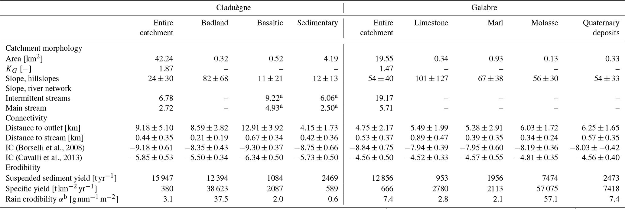
^a The values corresponding to the slope in the river network on the basaltic plateau and on sedimentary geology and are not limited to the erosion zones. ^b Rainfall erodibility corresponds to the mass of sediment detached on 1 m² by 1 mm of rain (Cea et al., 2016).

The 20 km² Galabre catchment is a headwater catchment of the Bléone River located in the southern French Alps (Fig. 1b). It is part of the Draix–Bléone Observatory dedicated to the study of hydrology and erosive processes in a mountainous context with extensive badlands. The climate of the Galabre catchment, whose altitude varies between 735 and 1909 m, is impacted by Mediterranean and mountainous influences with a mean annual precipitation of around 1000 mm. There is high seasonality, with most precipitation occurring in spring and autumn, although thunderstorms with high rain intensity also occur in summer (Esteves et al., 2019). The catchment is entirely located on sedimentary rocks comprising limestones (34 %), marls and marly limestones (30 %), gypsum (9 %), molasses (9 %) and Quaternary deposits (18 %). Prominent features of the catchment are the badlands that are found on all five types of rock and cover about 9.5 % of the surface of the catchment (Esteves et al., 2019). The land use is dominated by forests and scrublands, which are permanently covered by vegetation and are thus assumed to be negligible as sediment sources. Agricultural zones are barely present in the catchment. Suspended sediment fingerprinting studies have revealed that most of the sediments originate from the badlands of molasses and marls (Poulenard et al., 2012; Legout et al., 2013). Table 1 gives the characteristics of the catchment. In comparison, the Galabre catchment is smaller and steeper than the Claduègne catchment. The distribution of the erosion zones differs in the two catchments, with distributions in the Galabre catchment being more dispersed over the entire catchment but smaller in size due to the absence of diffuse agricultural sources.

Liquid and solid fluxes are continuously monitored at the outlets of both catchments with the same sensors and protocols, from which suspended sediment yields are calculated (Table 1). The water level is measured with an H radar and converted to discharge with a stage discharge rating curve. Suspended sediment concentrations are monitored with turbidimeters, and suspended sediment samples are automatically taken every 40 min once a threshold of turbidity and the water level is exceeded. These samples are dried, weighed, and used to establish a rating between turbidity and suspended sediment concentrations.

2.1.2 Connectivity indicators

In order to quantify the structural connectivity of the sources in the catchments, four indicators were calculated: the distance to the outlet, distance to the stream, and the two indices of connectivity (IC) proposed by Borselli et al. (2008) and Cavalli et al. (2013). The distance to the outlet metric refers to the width function and is applied as a measure of network structure and catchment shape by Hancock et al. (2010). Maps of the distance to the outlet along the flowlines (i.e., the distance that water and sediments travel following the gradient of the terrain elevation) and the distance to the stream were created. For the latter, the stream network obtained with a CDA threshold of 50 ha was used. The distance to the outlet and the distance to the stream of a given position in the catchment serve as proxies of longitudinal (upstream–downstream) and lateral (hillslope–channel) connectivity in the sense of Fryirs (2013). Both maps were created using TauDEM (Tarboton, 2010) and a digital elevation model at a resolution of 1m (Claduègne: bare Earth lidar DEM, Nord et al., 2017; Galabre: RGE ALTI product of IGN, 2018). However, neither of these measures takes into account surface roughness and slope. Thus, two of the most widely used indicators of connectivity, i.e., the IC proposed by Borselli et al. (2008) and the adjusted version of IC proposed by Cavalli et al. (2013), were calculated. Both indicators were calculated for each pixel of the DEM and take into account the CDA of that pixel and the distance to the stream along the flow lines. They also both include a weighting factor for the mean slope in the CDA and along the downstream path as well as a second weighting factor W. Borselli et al. (2008) weight the index with land use, and thus the factor W was derived from the values proposed by Panagos et al. (2014) for the land use data obtained from Inglada et al. (2017). Cavalli et al. (2013), on the other hand, propose a roughness index as the weighting factor W that represents a local measure of topographic surface roughness calculated for a 5×5 cell moving window. Both indicators were calculated using the program SedInConnect (Crema and Cavalli, 2018). All four indicators were calculated for each pixel within the catchments, and their values on the erosion zones were extracted. Mean values and standard deviations are given in Table 1, while the distributions of the distance to the outlet and to the stream are shown in Fig. 2. These characteristics of the catchments indicate that erodibility and also structural connectivity differ strongly between the two catchments and between sources.

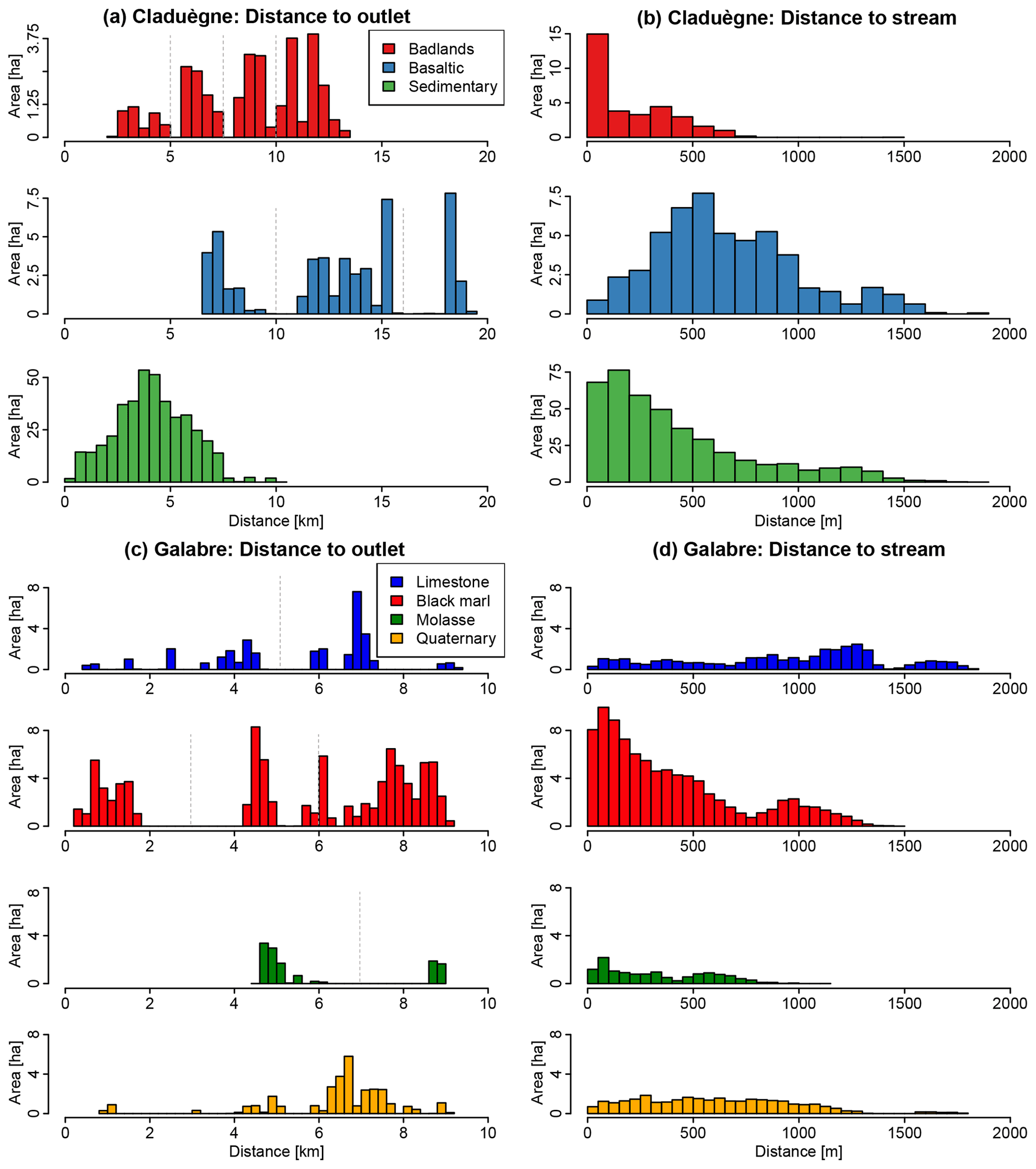
Figure 2 Distribution of the distance of the sources to the outlet (a for the Claduègne, c for the Galabre) and the stream (b for the Claduègne, d for the Galabre). The stream was defined with a threshold of contributing drainage area of 50 ha. The values represent distances along the flowlines that water and sediments travel following the gradient of the relief. Dashed grey lines correspond to the limits of subgroups of geological sources based on their distance to the outlet modeled in Sc. 4b and d.

2.2 Model description

Surface runoff, soil erosion, and sediment transport in the study catchments were modeled with an ad hoc version of the software Iber (Bladé et al., 2014) developed in a previous study by the authors (Cea et al., 2016). A detailed description of the model and numerical schemes is beyond the scope of this paper and can be found in previous publications. Thus, just a brief description of the model equations is presented in the following.

2.2.1 Hydrodynamic module

Water depth and velocity fields are computed from the solution of the 2D depth-averaged shallow-water equations applied to the whole catchment domain (including the hillslope and channel). Including rainfall and infiltration terms as well as Manning's formula for bed friction, the hydrodynamic equations solved by the model can be written as

$$\begin{array}{ll}{\displaystyle }& {\displaystyle \frac{\partial h}{\partial t}}+{\displaystyle \frac{\partial q_x}{\partial x}}+{\displaystyle \frac{\partial q_y}{\partial y}}=R-I\\ \text{(1)}& {\displaystyle }& {\displaystyle \frac{\partial q_x}{\partial t}}+{\displaystyle \frac{\partial }{\partial x}}\left({\displaystyle \frac{q_x^{\mathrm{2}}}{h}}\right)+{\displaystyle \frac{\partial }{\partial y}}\left({\displaystyle \frac{q_x{q}_y}{h}}\right)=-gh{\displaystyle \frac{\partial z_{\mathrm{s}}}{\partial x}}-g{\displaystyle \frac{n^{\mathrm{2}}}{h^{\mathrm{7}/\mathrm{3}}}}\left|q\right|q_x{\displaystyle }& {\displaystyle \frac{\partial q_y}{\partial t}}+{\displaystyle \frac{\partial }{\partial x}}\left({\displaystyle \frac{q_x{q}_y}{h}}\right)+{\displaystyle \frac{\partial }{\partial y}}\left({\displaystyle \frac{q_y^{\mathrm{2}}}{h}}\right)+=-gh{\displaystyle \frac{\partial z_{\mathrm{s}}}{\partial y}}-g{\displaystyle \frac{n^{\mathrm{2}}}{h^{\mathrm{7}/\mathrm{3}}}}\left|q\right|q_y,\end{array}$$

where h is the water depth, t is time, q_x and q_y are the components of the unit discharge in the two horizontal directions, R is the rainfall intensity, I is the infiltration rate, g is gravity acceleration, z_s is the elevation of the free surface, and n is Manning's roughness parameter. The shallow-water equations are solved with an unstructured finite-volume solver developed in Cea and Bladé (2015) for rainfall runoff applications at the catchment scale. The solver is explicit in time, meaning that the maximum time step that can be used to evolve the equations in time is limited by the Courant–Friedrichs–Lewy (CFL) condition (Courant et al., 1967). This implies that the time step in typical applications is of the order of 1 s or less. The CFL condition is implemented in the solver, and thus the computational time step is automatically evaluated from the grid size, water velocity, and water depth.

2.2.2 Soil erosion module

A full description of the soil erosion model can be found in Cea et al. (2016). The complete soil erosion model uses a two-layer soil structure that consists of one layer of eroded material over a layer of non-eroded cohesive soil. Different sediment classes, each one with its own physical properties, can be considered and routed with the model.

Given the results of Cea et al. (2016) that the two-layer structure of the model increases its complexity without significantly improving its predictive capacity in real applications, we only use a single-layer structure with vertically uniform erodibility. We assume that the single-layer structure is adequate for the badlands where there is usually a thick regolith layer, and erosion from the cohesive layer underneath is negligible compared to that of the regolith layer. In the complete model, two particle detachment processes are considered, i.e., rainfall-driven detachment and flow-driven entrainment. In our case, we assume that rainfall-driven detachment is the most significant of the two processes, and thus it is the only detachment mechanism considered in our simulations. We further assume that all eroded particles are transported in suspension to the outlet and that deposition is negligible. This wash load hypothesis leads to a further simplification of the erosion module compared to the original one proposed by Cea et al. (2016), i.e., the omission of the deposition term. Given the previous assumptions, the soil erosion model used in this work solves the following mass conservation equation for each sediment class considered:

$$\begin{array}{}\text{(2)}& {\displaystyle \frac{\partial h{C}_{\mathrm{s}}}{\partial t}}+{\displaystyle \frac{\partial q_x{C}_{\mathrm{s}}}{\partial x}}+{\displaystyle \frac{\partial q_y{C}_{\mathrm{s}}}{\partial y}}=D_{\mathrm{rdd},\mathrm{s}}s=\mathrm{1},N_{\mathrm{c}},\end{array}$$

where N_c is the number of sediment classes, C_s [kg m⁻³] is the depth-averaged concentration of the sediment class s, and D_rdd,s [$\mathrm{kg}{\mathrm{m}}^{-\mathrm{2}}{\mathrm{s}}^{-\mathrm{1}}$] is the rainfall-driven detachment rate for the sediment class s. The rainfall-driven detachment is calculated assuming a linear relationship between the detachment rate and the rain intensity, i.e., $D_{\mathrm{rdd},\mathrm{s}}={\mathit{\alpha }}_{\mathrm{s}}R$, where α_s [$\mathrm{g}{\mathrm{mm}}^{-\mathrm{1}}{\mathrm{m}}^{-\mathrm{2}}$] is the rainfall erodibility coefficient for the sediment class s and represents the mass flux detached per unit area by a unit of rainfall intensity. Thus, the suspended sediment concentration at every time step and location is calculated from Eq. (2), which is a simplified version of the equation given in Cea et al. (2016) for the case in which a single-layer structure, only rainfall-driven detachment, and no deposition are assumed. Equation (2) is solved with an unstructured finite-volume solver using the same spatial discretization as for the hydrodynamic equations. For a detailed description of the numerical schemes used to solve Eq. (2) coupled to the shallow-water equations, the reader is referred to Cea and Vázquez-Cendón (2012). The solution of Eq. (2) allows us to compute the concentration and thus the mass fluxes (as the product of the concentration times the unit discharge) of each sediment class at any time and location in the catchment, in particular, the contribution of each sediment class to the total sedigraph computed at the basin outlet.

2.3 Model discretization and input data

As a distributed model, Iber requires a computational mesh made up of three main modeling units with different spatial discretization and roughness coefficients, i.e., the river network, the hillslopes, and the badlands. The riverbed was delineated by (i) identifying the river network using TauDEM (Tarboton, 2010) and (ii) creating a polygon by “buffering” the line feature of the river. In order to take into account the fact that the width of the river varies from upstream to downstream, we introduced a distinction between the perennial river network defined using a CDA of 500 ha and the intermittent river network obtained using a CDA of 15 ha. While the highest value of 500 ha is often used for cartography and large-scale modeling studies (e.g., Colombo et al., 2007; Vogt et al., 2007; Bhowmik et al., 2015), the smallest value of 15 ha was found to create a river network that includes the intermittent streams observed in the catchment. For the former a buffer of 10 m to both sides of the river was applied. For the latter, composed of small tributaries and in good agreement with field observations of the whole extension of the hydrographic network during floods, a buffer of 5 m was applied. The badlands were delineated based on orthophotos and verified during field trips, while the hillslopes cover the rest of the catchments. While the badlands are part of the hillslopes in terms of geomorphology and hydraulics, we differentiated them here to be able to apply a different parameterization and discretization.

These principal modeling units were discretized as a finite-volume mesh. In our study, we used an unstructured triangular mesh with variable mesh size in the different units. The smallest mesh size was required in the modeling unit “river network”, in which water and sediment fluxes are concentrated, so it was set to 5 m. In the modeling unit “hillslopes” a coarser mesh size of 100 m was chosen in order to reduce the number of elements and thus computation time. In the modeling unit “badlands”, in which the fluxes are concentrated in the steep gullies, an intermediate mesh size of 20 m was used. At the border between two modeling units the mesh size evolves gradually. With this discretization the model of the Claduègne consists of roughly 173 000 mesh elements, while that of the Galabre catchment consists of 75 000 elements. Values for Manning's n and erodibility were assigned to each mesh element. The Manning's roughness parameter was uniform in each modeling unit but could vary from one scenario to another, with values ranging from 0.025 to 0.1 in the river network and from 0.2 to 0.8 in hillslopes and badlands. It was decided that the domain would get two Manning's values (channel vs. hillslope), i.e., a value for the modeling unit river network and another value for the modeling units hillslopes and badlands.

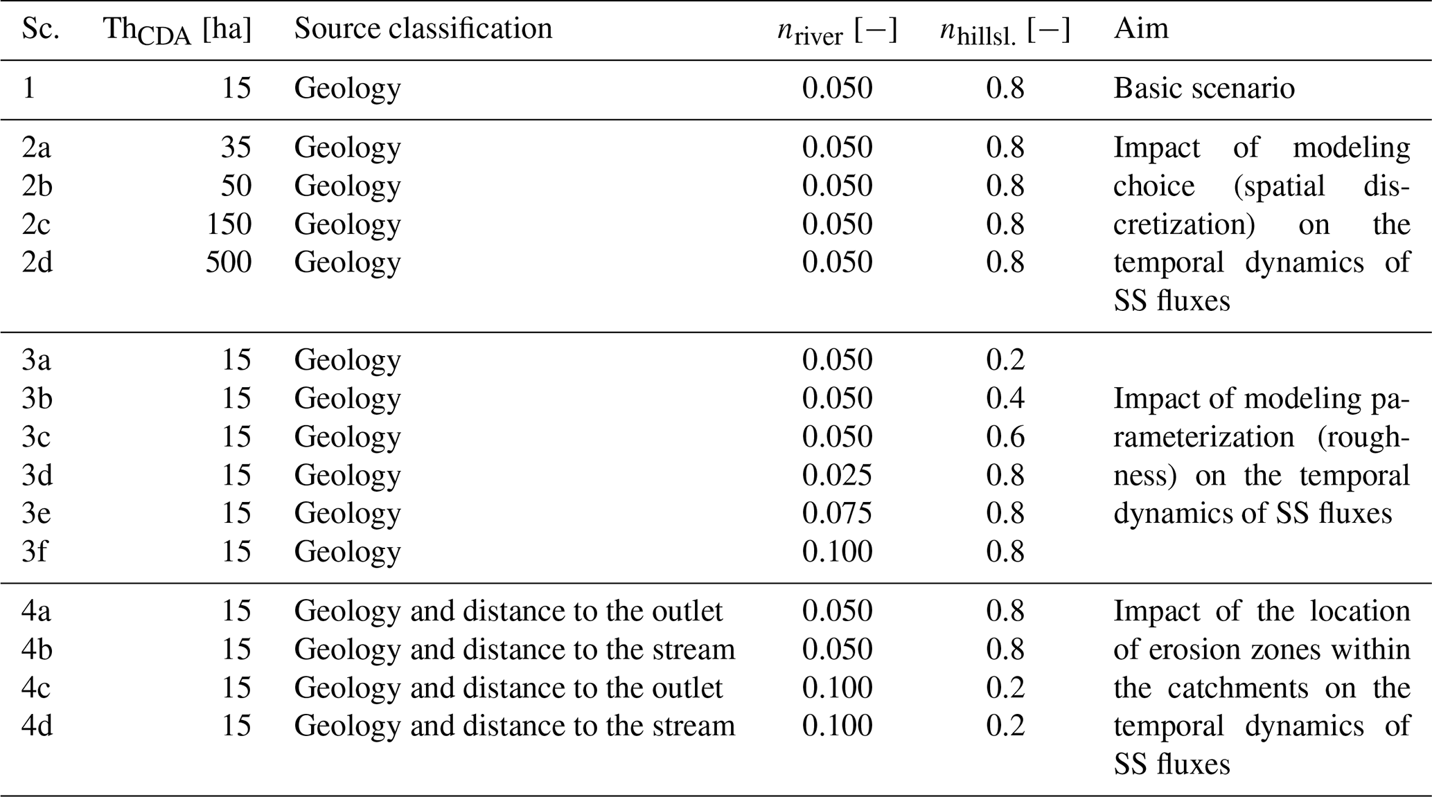
Table 2 Model scenarios (Sc.) detailed according to the value of the contributing drainage area threshold to define the river network (Th_CDA), the approach to classify the sources, the values for Manning's roughness parameter (n) in the river network and on the hillslopes, and the aim of the respective scenario.

While runoff is generated and routed in the entire catchment, the production of sediment was limited to the potential erosion zones. The latter include all the mesh elements in the modeling unit badlands and the mesh elements of the hillslopes modeling unit that belonged to the diffuse agricultural sources in the Claduègne catchment. The erosion zones were classified according to (i) their geology, i.e., in three classes for the Claduègne and four for the Galabre catchment (Fig. 1), (ii) their geology and their distance to the outlet (Fig. 2a and c), and (iii) their geology and their distance to the stream network (Fig. 2b and d). Sediment production (D_rdd,s) was calculated in each mesh element of the potential erosion zones for each source class separately. Sediment transfer (Eq. 2) was then routed over the entire catchment. Thus, separate sedigraphs for each source class were obtained at the outlet of the catchment, and the contribution of each source class to total sediment flux could be calculated for every time step. The rain erodibility coefficient α of each geological class was estimated from the available observed time series of suspended sediment concentrations (SSCs), discharge, and rainfall. Using the discharge and SSC, the suspended sediment flux was calculated and integrated over time for each recorded event to obtain event suspended sediment yield SSY_ev [g]. The value of α [$\mathrm{g}{\mathrm{mm}}^{-\mathrm{1}}{\mathrm{m}}^{-\mathrm{2}}$] was estimated separately for every event and every source as

$$\begin{array}{}\text{(3)}& {\mathit{\alpha }}_{\mathrm{s},\mathrm{ev}}={\displaystyle \frac{{\text{SSY}}_{\mathrm{s},\mathrm{ev}}}{R_{\text{ev}}\cdot A_{\mathrm{s}}}},\end{array}$$

where A_s is the erodible surface of the respective source and R_ev [mm] is the amount of effective rainfall during the respective event. SSY_s,ev is the contribution of source s to SSY_ev and was calculated based on the mean source contributions. They were estimated with sediment fingerprinting in the Claduègne catchment by Uber et al. (2019) and in the Galabre catchment by Legout et al. (2013). An average value of α_s was calculated by averaging over all the available observed events (Table 1). As the focus of this study is on choices made during model setup and how structural connectivity is represented, a synthetic triangular hyetograph (duration of 12 h, maximum intensity of 5 mm h⁻¹) representing effective precipitation (i.e., R−I) is spatially homogeneously applied over the entire catchment. The simulated time is 24 h, including 12 h of rain and 12 h for the fluxes to reach the outlet.

2.4 Study design and modeling scenarios

To achieve the first objective dealing with the impact of modeling choices on the temporal dynamics of modeled hydrosedimentary fluxes, a one-factor-at-a-time sensitivity analysis (Pianosi et al., 2016) was conducted. The model was set up and parameterized in a basic scenario (Table 2, Sc. 1), and then subsequently two different input factors were varied: the CDA threshold to define the river network (Sc. 2) and Manning's roughness parameter n (Sc. 3). Based on preliminary studies that are not reported here, these two factors were found to be the most important ones in determining sediment flux dynamics. While other factors (erodibility, rainfall intensity) crucially influence absolute values of erosion and suspended sediment concentration, their values are less important to determine arrival times and temporal dynamics of source contributions. For the second objective dealing with the impact of the location of erosion zones, indicators of structural connectivity of the two catchments are used to describe the configuration of each sediment source in the catchments. They are compared to the modeled hydrosedimentary fluxes both qualitatively by visual analyses and quantitatively by means of the calculation of characteristic times of the hydrographs and sedigraphs (e.g., time of concentration, lag time). To this end, another set of scenarios was generated wherein the sediment sources were subdivided into more or less connected zones (Table 2, Sc. 4).

The underlying hypothesis is that both modeling choices (notably CDA threshold and Manning's n) and catchment characteristics (structural connectivity of the sources) determine travel times from the sources to the outlet. With the presented study design, it could be assessed whether modeling choices or actual catchment configurations were more important in generating temporal variability in sediment outputs.

2.4.1 Sc. 1: basic scenario

In the basic scenario the threshold to define the river network was set to 15 ha and the sources were classified according to their geology as in the sediment fingerprinting studies. In the river network modeling units, Manning's n was set to 0.05, and in the hillslopes and badlands modeling units it was set to 0.8. The value in the river network corresponds to what can be expected from values reported in the literature for streams comparable to the Claduègne and the Galabre (Te Chow, 1959; Barnes, 1967; Limerinos, 1970). For the values on the hillslopes there are fewer recommendations from the literature as the use of the St. Venant equations for the calculation of fluxes on hillslopes is much less common. Existing studies indicate that the values have to be considerably higher than those used commonly in river flow models (Engman, 1986; Hessel et al., 2003; Fraga et al., 2013; Hallema et al., 2013). As these values are uncertain, the impact of this parameterization was assessed in further scenarios. The basic scenario was used as the main reference to which to compare the other scenarios and for the comparison between the two catchments.

2.4.2 Sc. 2: impact of the CDA threshold

We tested the impact of varying the CDA threshold on the modeled hydrosedimentary response while keeping all other parameters unchanged compared to the basic scenario (one-factor-at-a-time sensitivity analysis). As different values for Manning's n were applied in the river network modeling unit and in the hillslopes and badlands modeling units, the travel times of the sediments from source to sink vary depending on the length of the river network in the model. Thus, it can be assumed that modeled sediment dynamics are sensitive to this parameter. Five values of the CDA threshold were used: 15, 35, 50, 150, and 500 ha.

Sc. 3: impact of the parameterization of Manning's n

As the first objective of this study is to assess the impact of choices made during model setup on the simulated sediment flux dynamics, the model was run with different values of Manning's n in the river network modeling unit and in the hillslopes and badlands modeling units. In the river network units, values were varied spanning a range from 0.025 to 0.100. This corresponds to the full range of plausible values (Te Chow, 1959; Limerinos, 1970). In the hillslopes and badlands modeling units, the value of 0.8 used in the basic scenario is already at the upper end of values reported in the literature (e.g., Te Chow, 1959; Engman, 1986; Hessel et al., 2003; Hallema et al., 2013). Thus, values in the range of 0.2 to 0.8 were tested.

2.4.3 Sc. 4: source classification based on connectivity

In order to test how the spatial distribution of the sources in the two distinct catchments contributes to the modeled sedigraph at the outlet, the geological sources were classified into subclasses based on their distance to the outlet (Sc. 4a, c) and distance to the stream (Sc. 4b, d). These two measures serve as a proxy for the structural connectivity of the sources. The underlying hypothesis is that depending on their connectivity, several patches of the same source have different travel times to the outlet and can therefore lead to several peaks in the sedigraph of the source. In Sc. 4b and d, the geological sources were classified into two groups based on their distance to the stream. The badland sources in both catchments were classified as being directly adjacent to the stream network or not. The diffuse sources in the Claduègne catchment, i.e., cultivated soils on basaltic and sedimentary geology, were classified using a threshold of distance to the stream of 150 m. In Sc. 4a and c, the geological sources were classified into one to four groups depending on their distribution of distance to the outlet (Fig. 2a and c). Besides the values for Manning's n used in the basic scenario, in Sc. 4c and d we used values for Manning's n with less contrast between the hillslopes and the river network. This was done to assess whether the interpretation of Sc. 4a and b depended on the values of n. It should be stressed that this source classification does not influence model physics; i.e., total sediment yield from a source (close and distant sources) remains the same as in the basic scenario in which they are not differentiated.

2.5 Comparison of scenarios

Modeled outputs for each scenario can be accessed and visualized through Uber et al. (2020). To assess the impact of the changes made in each scenario with respect to the basic scenario, several characteristics of the modeled hydrograph and sedigraphs of all sources were calculated. The lag time of liquid discharge $T_{\text{lag},Q_{\mathrm{l}}}$ is calculated as the time between the barycenter of the hyetograph and the barycenter of the hydrograph. The time of concentration of liquid discharge $T_{\mathrm{c},Q_{\mathrm{l}}}$ is defined as the time between the end of effective precipitation and the end of the outlet hydrograph. A third characteristic time, $T_{\text{spr},Q_{\mathrm{l}}}$, was defined to assess the spread of the hydrograph and thus a characteristic duration of the flood event (Fig. 3). All of these measures were also calculated for solid discharge ($T_{\text{lag},Q_{\mathrm{s}}}$, $T_{\mathrm{c},Q_{\mathrm{s}}}$, $T_{\text{spr},Q_{\mathrm{s}}})$ and for each source separately. Further, maximum liquid discharge Q_l,max and solid discharge Q_s,max were determined for each scenario. Our simulations were truncated 12 h after the end of precipitation and in some cases fluxes did not recede to zero, so a threshold of 0.1 Q_max was used to calculate T_lag, T_c, and T_spr for solid and liquid discharges. We use these metrics to quantitatively assess differences in model output between the scenarios described above.

Figure 3 Scheme of the calculation of characteristic times T_lag, T_c, and T_spr that were calculated using the simulated liquid and solid discharges. The points represent the barycenter of the hyetograph (blue curve) and of the fraction of discharge above the threshold of 0.1Q_max (black curve).

3 Results and discussion

3.1 Impact of modeling choices on modeled sediment dynamics

3.1.1 Varying the contributing drainage area threshold

Results show that modeled hydrographs and sedigraphs were sensitive to the choice of the CDA threshold used to define the river network. Figure 4 shows the modeled hydrographs that were obtained when the CDA threshold was varied from 15 to 500 ha. For both catchments, higher values led to a less steep rising limb of the hydrograph, lower and later peak flow, slower recession, and a flatter hydrograph (Fig. 4a and c). Thus, the lag time T_lag, time of concentration T_c, and time of spread T_spr of liquid discharge increased with an increasing CDA threshold (Fig. 5a–c; Table 3). In both catchments, the hydrographs obtained with thresholds of 15, 35, and 50 ha were relatively similar, but the results obtained with 150 and 500 ha differed considerably. In the Claduègne catchment peak flow was reduced by approximately a factor 2 when the threshold was increased from 15 to 500 ha, while in the Galabre catchment it decreased by about 20 % (Table 3). In the Claduègne catchment the hydrograph obtained with the threshold of 500 ha was much flatter than the one in the Galabre catchment, and the recession was very slow so that even 12 h after the end of precipitation, discharge at the outlet persisted. This was not the case in the Galabre catchment.

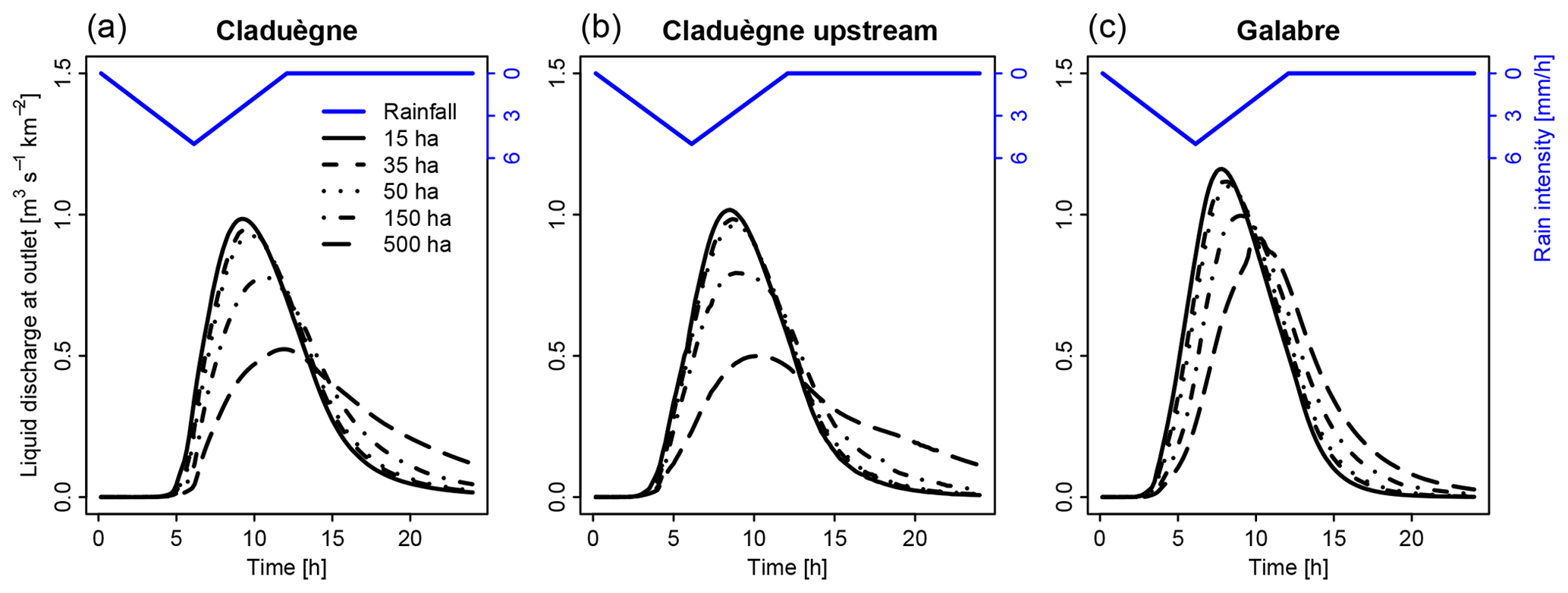
Figure 4 Simulated specific discharge obtained with different scenarios of model discretization at the outlet of (a) the 42 km² Claduègne catchment and (b) the 20 km² upstream outlet of the Claduègne where the size of the subcatchment is the same as that of (c) the Galabre catchment. The threshold for defining the river network is varied from 15 to 500 ha.

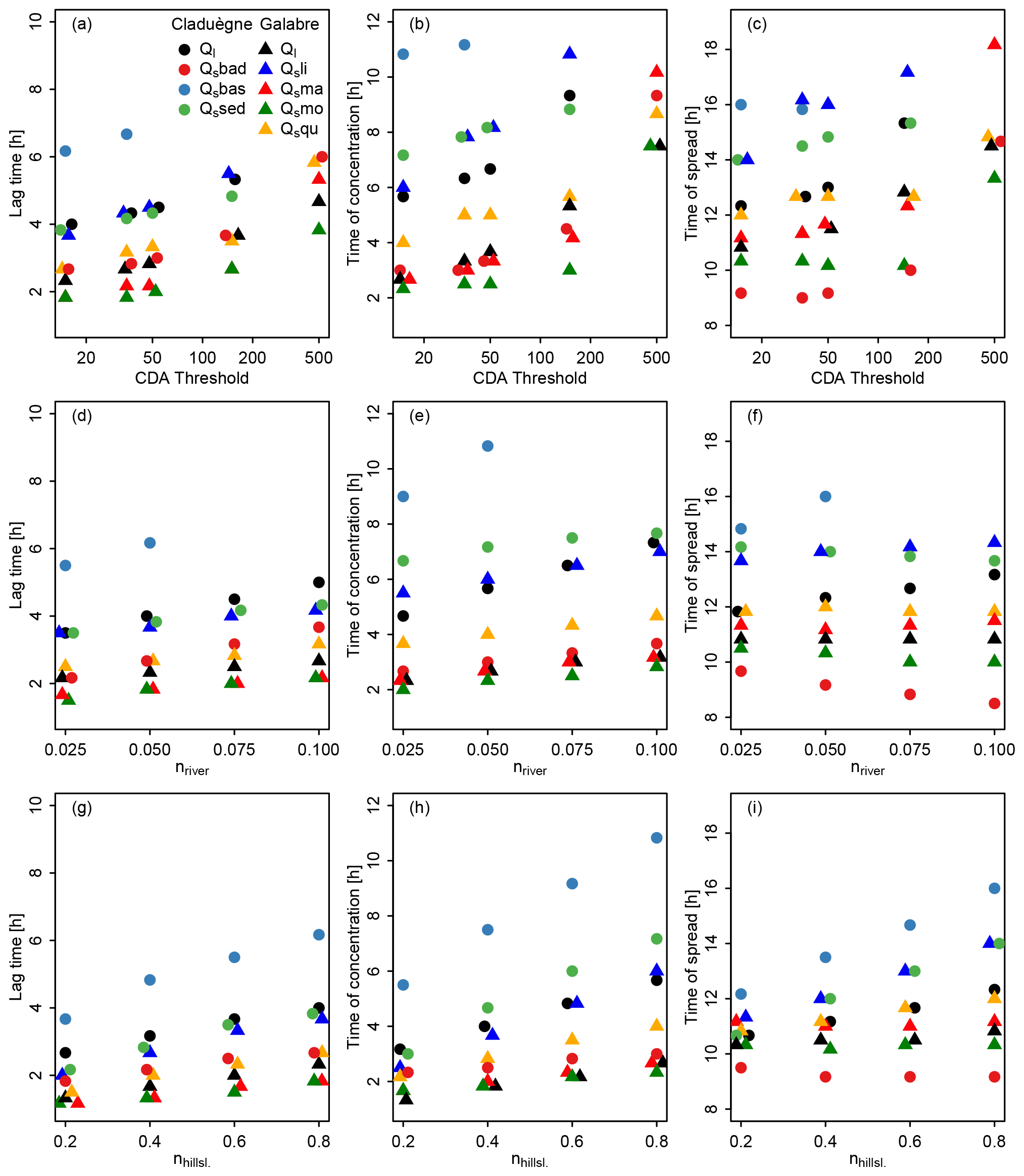
Figure 5 Sensitivity of lag times, times of concentration, and time of spread to changing the CDA threshold (a–c), Manning's n in the river network (d–f) and on the hillslopes (g–i). For each catchment the characteristic times are given for liquid discharge (Q_l) and for solid discharge (Q_s) of the different source classes. Some symbols were slightly shifted on the x axis if they were hard to see or overlapped other symbols.

Table 3 Calculated characteristics of modeled hydrographs and sedigraphs for the different scenarios. Abbreviations are as follows. $T_{\text{lag},Q_{\mathrm{l}}}$: lag time of liquid discharge, $T_{\mathrm{c},Q_{\mathrm{l}}}$: time of concentration of liquid discharge, $T_{\text{spr},Q_{\mathrm{l}}}$: spread of the hydrograph, Q_l,max: peak of liquid discharge. Q_s refers to solid discharge, and the characteristic times are calculated for each source separately (i.e., badlands, basaltic, and sedimentary in the Claduègne catchment; limestone, black marl, molasses, and Quaternary deposits in the Galabre catchment). The background color of the cells represents the percent change of each value with respect to the basic scenario. NA values indicate that the hydrograph or sedigraph did not recede to 0.1Q_max within the simulated time.

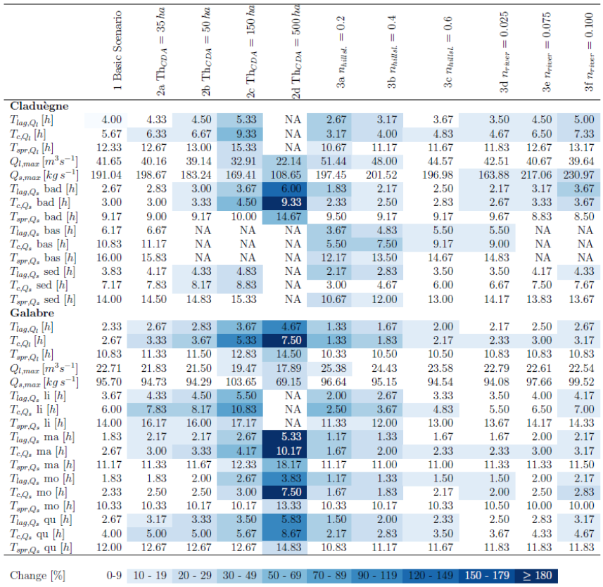
The different hydrological response could not be attributed to the difference in size of the catchments alone because a subcatchment of the Claduègne that has the same size as the Galabre catchment and a similar mean slope as the entire Claduègne catchment (mean±SD: 25±32 %) also had a less steep rising limb of the hydrograph than the Galabre (Fig. 4b). The T_lag of 3.2 h (basic scenario) was smaller than that of the Claduègne catchment at the outlet (4 h) but also considerably larger than that of the Galabre catchment (2.3 h). Thus, we assume that the fast rise and recession of the hydrograph in the Galabre catchment were mainly due to the steeper slopes in this catchment (Table 1) given that the lengths of the river networks are similar. This is coherent with the presumption that catchment response times are negatively correlated with catchment slopes (Gericke and Smithers, 2014). The modeled responses of the sedigraphs were also very sensitive to the CDA threshold. T_lag, T_c, and T_spr of solid discharge generally increased with an increasing CDA threshold, in particular from 150 to 500 ha (Fig. 5a–c; Table 3). Nevertheless, the changes in CDA did not affect the sedigraphs similarly for each sediment source. In the Claduègne catchment, the sedigraphs obtained with CDA thresholds of 15, 35, and 50 ha were similar to each other, but when larger values were used, they varied substantially for each sediment source (Fig. 6a–d). In particular, the sedigraphs of the basaltic and sedimentary sources were considerably delayed when the 500 ha threshold was used. In the Galabre catchment the sedigraphs of all sources were highly sensitive to significant changes in the CDA threshold with changes in $T_{\text{lag},Q_{\mathrm{s}}}$ and $T_{\mathrm{c},Q_{\mathrm{s}}}$ of more than 100 % for the CDA threshold of 500 ha (Table 3). When the threshold of 500 ha was used, the shape of the sedigraph of some sources differed. Indeed, for the badlands in the Claduègne catchment and the black marls and the molasses in the Galabre catchment, the single-peak sedigraph turned into a multi-peak sedigraph (Fig. 6).

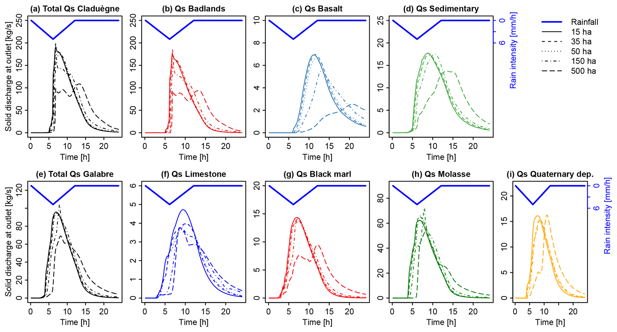
Figure 6 Simulated sedigraphs for total suspended solid discharge (Q_s) and for each source in the two catchments when different values are used for the threshold of contributing drainage area (CDA) to define the river network.

The differences in the modeled sedigraphs when different values for the CDA threshold were used were also obvious when the simulated contributions of the sources to total suspended sediment load were regarded (Fig. 7 and interactive figures at https://shiny.osug.fr/app/EROSION_MODEL.2020, last access: 2 March 2021). Increasing the CDA threshold from 15 to 500 ha notably prolonged the first flush of black-marl-dominated sediment in the Galabre catchment (marked as 1 in Fig. 7c, d). During the rising limb of the hydrograph and peak flow (marked as 2), the source contributions were variable, while they remained relatively constant during the recession period (3) when the CDA threshold of 500 ha was used. This was not the case when the threshold was set to 15 ha. In this case, the contribution of molasses decreased steadily throughout the event, while that of limestone and Quaternary deposits increased (2, 3, and 4 in Fig. 7c). In the Claduègne catchment the arrival of the basaltic sources at the outlet was notably delayed when the CDA threshold of 500 ha was used compared to when 15 ha was used. The shape of the sedigraph with multiple peaks that was modeled with a threshold of 500 ha resulted in a slower and less steady recession of the badland sources (Fig. 7b).

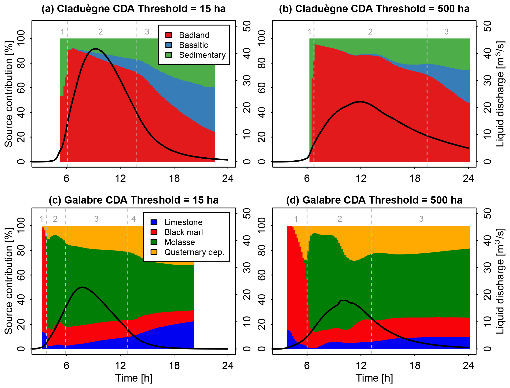
Figure 7 Modeled source contributions of the sediment sources in the Claduègne and Galabre catchments when the threshold of contributing drainage area (CDA) is set to 15 ha (a and c, Sc. 1) or to 500 ha (b and d, Sc. 2d). The color shows the contribution of the different sources to total suspended sediment load in percent. The hydrograph is additionally shown to represent the timing of the event. The results obtained with all five CDA thresholds (15, 35, 50, 150, and 500 ha) for both catchments can be visualized in interactive figures at https://shiny.osug.fr/app/EROSION_MODEL.2020 (last access: 2 March 2021).

Overall, our results showed that the thresholds of 15, 35, and 50 ha produced very similar results. Thus, in this range, the model was not very sensitive to the CDA threshold. The parameters given in Table 3 changed by a maximum of 37 % compared to the basic scenario. Other authors have shown that the CDA thresholds can vary spatially (i.e., different values are found in different subcatchments) and temporally (CDA thresholds vary between seasons or between events; Montgomery and Foufoula-Georgiou, 1993; Bischetti et al., 1998; Colombo et al., 2007). In the studied catchments, variability in this range seemed not to be of prime importance. However, the larger thresholds of 150 and 500 ha changed the modeled sediment dynamics considerably (changes of up to 280 % with respect to the basic scenario and several parameters changed>150 %; Table 3). This result showed that it is important to use a CDA threshold that is of the same order of magnitude as the value that produces a realistic river network. Field observations or detailed maps (i.e., topographic map at scale 1:25 000) can be valuable sources of information for this purpose. The sensitivity of model output to variations of the CDA threshold was also observed by other authors (Pradhanang and Briggs, 2014). For our modeling setup it is reassuring that model results converged when the CDA threshold used was derived from field observations.

Varying Manning's n

Changing Manning's n influenced the timing, the peak, and the spread of both liquid discharge and total suspended sediment load (Fig. 8, Table 3). In general, increasing n_river and n_hillsl. led to a later time of rise of the hydrograph, a later time of peak, and a slower recession with longer $T_{\text{lag},Q_{\mathrm{l}}}$ and $T_{\mathrm{c},Q_{\mathrm{l}}}$ (Fig. 5, Table 3). Nevertheless, Q_l,max, $T_{\text{lag},Q_{\mathrm{l}}}$, $T_{\mathrm{c},Q_{\mathrm{l}}}$, and $T_{\text{spr},Q_{\mathrm{l}}}$ were less sensitive to changes in n_river and n_hillsl. in the Galabre than in the Claduègne catchment (Fig. 5, Table 3). While increasing n also led to less maximum liquid discharge, this was not the case for solid discharge. Peak solid discharge even increased with increasing n_river in the Claduègne catchment and to a lesser degree also in the Galabre catchment (Table 3). Interestingly, in the Claduègne catchment liquid discharge was more sensitive to changes in n_hillsl. than to n_river, while solid discharge was more sensitive to n_river. This was not the case in the Galabre where both liquid and solid discharges were more sensitive to n_hillsl..

Changing Manning's n also influenced the temporal dynamics of source contributions. A low n_hillsl. of 0.2 led to a multi-peaked sedigraph in the Claduègne catchment (Fig. 8b). This difference in the shape of the sedigraph also led to a difference in the modeled temporal dynamics of the percentage of source contributions (Fig. 9a). When n_hillsl. was set to 0.2, the decrease of the contribution of the badland sources to total suspended sediment load in the Claduègne catchment was slower during the main part of the event (marked 2 in Fig. 9a), and the break point between phase 2 and 3 in the decrease in the badland source was more pronounced than in the basic scenario in which n_hillsl. was set to 0.8 (Fig. 7a). In fact, for several hours during phase 2, the contributions of the three sources were nearly constant. This was not the case for scenarios 3b and c in which n_hillsl. was set to 0.4 and 0.6. These scenarios hardly differed from the basic scenario (see interactive figures). In the Galabre catchment scenarios 3b and c also hardly differed from the basic scenario. When n_hillsl. was set to 0.2, the contributions during the main part of the event (2 in Fig. 9b) remained more stable in time than in the basic scenario (Fig. 7c).

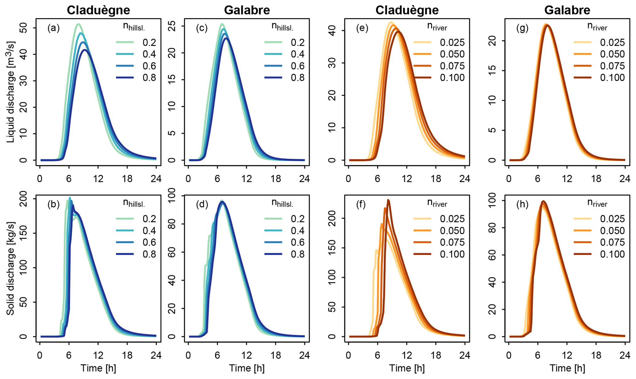
Figure 8 Sensitivity of modeled hydrographs (a, c, e, g) and sedigraphs (b, d, f, h) to changing Manning's roughness parameter on the hillslopes (a–d) and in the river network (e–h). For panels (a–d) n_river was fixed to 0.05. For panels (e–h) n_hillsl. was fixed to 0.8.

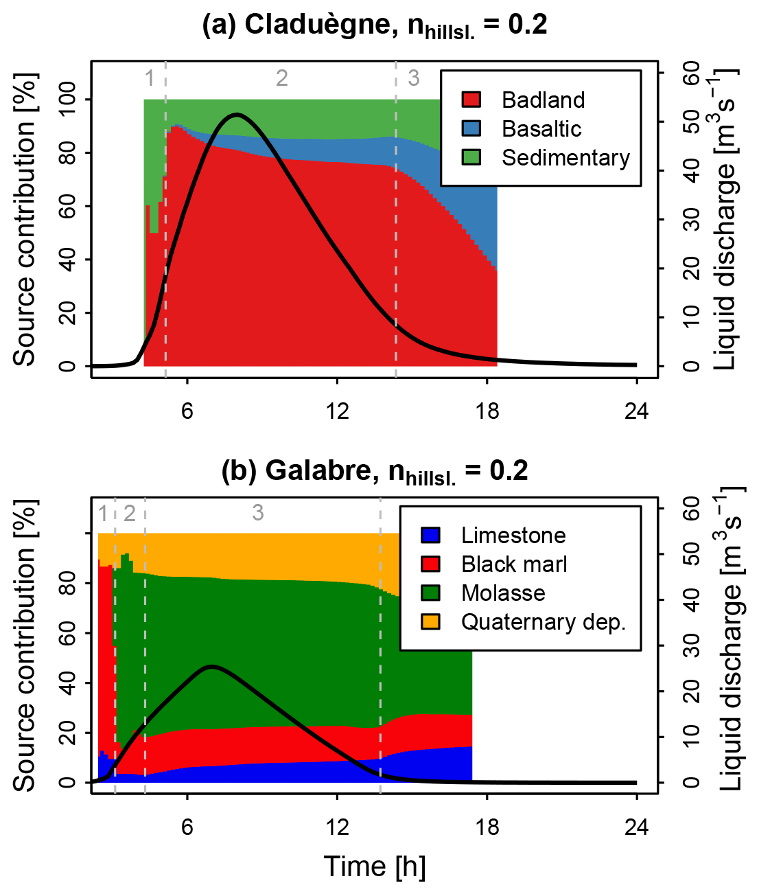
Figure 9 Modeled contributions of the sediment sources in the two catchments when Manning's n on the hillslopes was set to 0.2 (Sc. 3a). The color shows the contribution of the different sources to total suspended sediment load in percent. The hydrograph is additionally shown to represent the timing of the event. The results obtained with all roughness values for both catchments can be visualized in interactive figures at https://shiny.osug.fr/app/EROSION_MODEL.2020 (last access: 2 March 2021).

Changing n_river hardly changes the dynamics of the modeled source contributions in both catchments (see interactive figures). In the Claduègne catchment, increasing n_river from 0.025 to 0.1 generally increased $T_{\text{lag},Q_{\mathrm{s}}}$ and $T_{\mathrm{c},Q_{\mathrm{s}}}$ (Fig. 5, Table 3) and led to a slight prolongation of the first flush of sediments from the sedimentary source. In the Galabre this was also the case for the first flush of sediments originating from black marl, as was the case for the changes in the CDA threshold shown in Fig. 7d.

Our results showed that even though modeled liquid discharges were sensitive to n_hillsl. (e.g., maximum liquid discharge changed by 24 % in the Claduègne catchment and 12 % in the Galabre catchment), the sedigraphs of the main sources and thus of total suspended solid discharge were much less sensitive to this parameter (maximum solid discharge changed by 3 % in the Claduègne catchment and by 1 % in the Galabre catchment; Fig. 8). This was due to the fact that in both catchments the main sediment sources were located close to the river (Table 1, Fig. 2). Thus, only a small fraction of the trajectory of particles was located on the hillslopes. This was also represented in the modeled dynamics of the source contribution, which barely changed unless the most extreme value of 0.2 was applied. This result suggests that it is sufficient to have a rough idea of the value of Manning's n to study the dynamics of sediment fluxes. In the Claduègne catchment the modeled sedigraph was affected by variations of n_river, which was less true for the Galabre catchment. This might be related to the difference in the slopes of the river network in the two catchments. Indeed, the mean slope in the river network is 2–3 times higher in the Galabre than in the Claduègne catchment (Table 1), suggesting that the model was more sensitive to changes in Manning's n when slopes were low. However, also in the Claduègne catchment, changes in n_river did not change the modeled dynamics of the source contributions, which was again encouraging for the use of this type of model to understand hydrosedimentary dynamics.

3.2 The role of structural connectivity in the dynamics of suspended sediment fluxes at the outlet

The application of the same rainfall event with a similar spatial discretization and parameterization to the two studied catchments (i.e., basic scenario) allowed us to provide a more detailed analysis of how their respective characteristics influenced their hydrosedimentary response. A first result was that the Galabre catchment reacted faster than the Claduègne catchment. The hydrographs and the sedigraphs rose earlier than in the Claduègne catchment. We assume that this was mainly due to the steeper slopes of the Galabre catchment (Table 1). From Figs. 7 and 9, a general pattern of the contribution of the different geological sources to total suspended sediment load can be derived: in the Claduègne catchment at the onset of the event (1), the sediments originated from the sedimentary source and the badlands. During phases 2 and 3 of the event, the main source (i.e., the badlands; Table 1) clearly dominated total suspended sediment load. The contribution of this source decreased gradually, while the percentage of contribution of the two others increased. In the Galabre catchment at the onset of the event (1), suspended sediment originated almost entirely from the black marls, i.e., the source closest to the outlet. In the second phase of the event, the main source (i.e., molasse) arrived and clearly dominated total suspended sediment load. Thereafter, the contribution of the molasses decreased, while that of the limestones and the Quaternary deposits increased (phases 3 and 4). These general patterns were broadly consistent with the location of the different geological sources in the two catchments. However, some discrepancies appear when comparing the timing of arrival of the various geological sources to the ranking of the various connectivity indicators (i.e., distance to stream, to outlet, IC Borselli, and IC Cavalli). The lag times of the sources in the Claduègne catchment could generally be ranked as $T_{\text{lag},Q_{\mathrm{s}}}\text{bad}<T_{\text{lag},Q_{\mathrm{s}}}\text{sed}<T_{\text{lag},Q_{\mathrm{s}}}\text{bas}$ (Table 3, Fig. 5). This was also true for $T_{\mathrm{c},Q_{\mathrm{s}}}$ and $T_{\text{spr},Q_{\mathrm{s}}}$, and this is consistent with the ranking of the mean distance to the stream as well as with both mean IC values but not with the mean distance to the outlet, as the sedimentary sources were the closest to the outlet (Table 1). In the Galabre catchment $T_{\text{lag},Q_{\mathrm{s}}}$, $T_{\mathrm{c},Q_{\mathrm{s}}}$, and $T_{\text{spr},Q_{\mathrm{s}}}$ of the molasses and marls were always smaller than those of Quaternary deposits and limestones (basic scenario, Table 3). This was coherent with the ranking of mean distances to the stream but not with the ranking of mean distances to the outlet or the mean IC values (Table 1). Actually, the mean IC values in the Galabre were very similar for each of the four geological sources of sediments and could not really be used to discriminate the sources in terms of the timing of arrival of the sedigraphs at the outlet.

To further address the respective roles of the distance to the outlet and the distance to the stream in the pattern of source contributions to total suspended sediment load throughout events, the geological sources were subdivided based on these measures in scenarios 4a to b (Table 2). In this way, model output consisted of separate sedigraphs for the close and distant subsources of a given source class. The sum of these sedigraphs is the same as the sedigraph of that source class in the basic scenario. Figures 10 and 11 show for the Galabre catchment that the limestone sources that were close to the river and the ones that were close to the outlet exhibited a clockwise discharge–sediment flux hysteresis pattern, while the distant ones exhibited an anticlockwise pattern. These results confirm the typical interpretations of hysteresis loops, i.e., the assumption that clockwise loops indicate a dominance of close sources because maximum sediment flux occurs before peak discharge, while anticlockwise hysteresis patterns indicate a dominance of more distant sources (Bača, 2008; Misset et al., 2019). The results further highlight the fact that the sedigraphs of the different sediment sources are strongly related to their location in the catchments and their structural connectivity. The absence of coherent trends in the ranking of the $T_{\text{lag},Q_{\mathrm{s}}}$ relative to the mean distances of the sources to the outlet could be related to the distribution of the distances to the outlet of all sediment sources that were generally more scattered than the distribution of the distances to the stream, particularly for the Galabre catchment (Fig. 2c and d). Thus, the mean distance to the outlet was not sufficient to determine travel times of the sources to the outlet. Additionally, the triangular rain applied to both catchments had a rather long duration that was much longer than the concentration times of both catchments. Thus, the sedigraphs of all subsources were stretched over a time span that was comparable to the time span of the rain event. The distant sources arrived at the outlet long before the flux of the close sources ceased. Consequently, the sedigraphs of the different subsources of both catchments were superposed and did not lead to separate peaks.

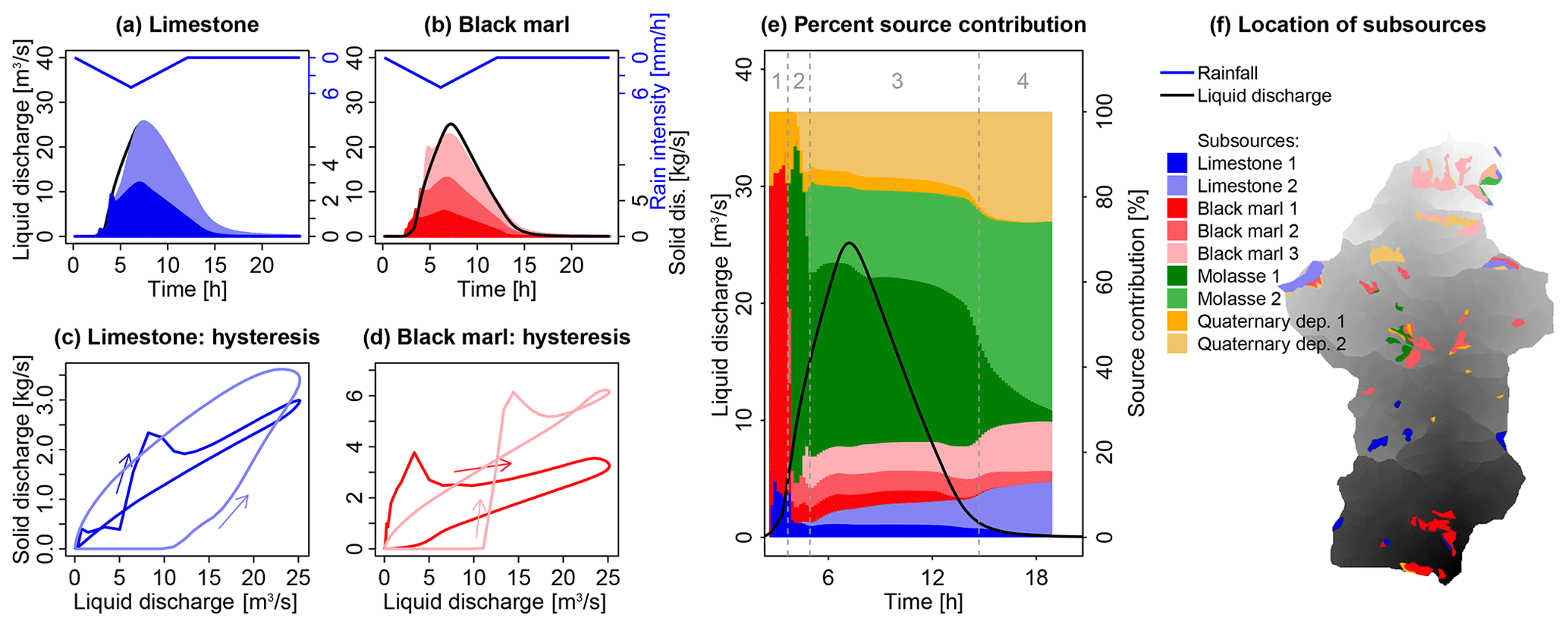
Figure 10 (a, b) Contribution of subsources of limestone and black marl that are classified according to their distance to the outlet (Sc. 4a). The colored areas show the contribution of sources close to the outlet (darker colors) and more distant sources (lighter colors) from the sedigraph. (c, d) The hysteresis loops of the subsources. (e) The contribution of each subsource to total suspended solid discharge in percent. The dashed lines and the grey numbers above the figure distinguish different periods of the event as referred to in the text. (f) Location of the subsources in the Galabre catchment.

Figure 11 Contribution of subsources that are classified according to their distance to the stream in the Galabre catchment (Sc. 4b). For a description of the panels, see the caption of Fig. 10.

Even though different patches of closer and more distant subsources did not lead to multi-peak sedigraphs and thus to a very high flux variability, the classification into close and distant subsources relative to the outlet allowed us to explain the dynamics of source contributions. The first peak of black marls that arrived at the outlet of the Galabre during the onset of the event originated entirely from the subsources that were close to the outlet and adjacent to the river network (marked 1 in Figs. 10e and 11e). For the molasses and Quaternary deposits, the distance to the river or the outlet hardly impacted the variability of the predicted source contributions. The first molassic sediments that arrived at the outlet during the rise of the hydrograph (2) originated almost entirely from the molassic patch that was directly adjacent to the river network. However, the decrease in the contribution of the adjacent sources during peak flow (3) occurred simultaneously with the arrival of the further sources.

A similar dynamic was observed in the Claduègne catchment. The first flush of sediments with a high contribution from the sedimentary source originated entirely from sedimentary sources that were directly adjacent to the stream and from the badlands that were closest to the outlet (marked 1 in Figs. 12e and 13e). When the results were analyzed in terms of the distance to the outlet, it was remarkable that sediments which originated from the class badland 3 (corresponding to a distance to the outlet of 7.5–10 km; $T_{\text{lag},Q_{\mathrm{l}}}=\mathrm{2.17}$ h) arrived during the rising limb of the hydrograph (2) before the ones that originated from badland 2 (distance to the outlet 5–7.5 km; $T_{\text{lag},\text{Ql}}=\mathrm{2.67}$ h) even though they were further away from the outlet. This was coherent with the distance to the stream. While all patches belonging to the class badland 3 were directly adjacent to the river network, the ones belonging to the class badland 2 were further away from the river. It should be stressed, however, that this finding is related to the parameterization of the model and the choice of using contrasting roughness coefficients on hillslopes and in the river. In the results of Sc. 4c in which n_river was set to 0.1 and n_hillsl. was set to 0.2 (i.e., less difference between n_river and n_hillsl.), this was not observed.

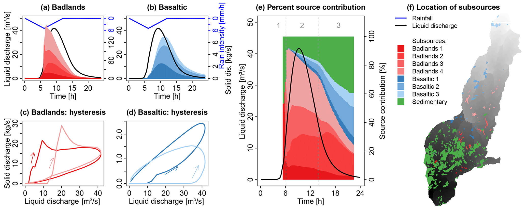
Figure 12 (a, b) Contribution of subsources of badlands and basaltic sources that are classified according to their distance to the outlet (Sc. 4a). The colored areas show the contribution of sources close to the outlet (darker colors) and more distant sources (lighter colors) from the sedigraph. (c, d) The hysteresis loops of the subsources. (e) The contribution of each subsource to total solid discharge in percent. The dashed lines and the grey numbers above the figure distinguish different periods of the event as referred to in the text. (f) Location of the subsources in the Claduègne catchment.

Figure 13 Contribution of subsources that are classified according to their distance to the stream in the Claduègne catchment (Sc. 4b). For a description of the panels, see the caption of Fig. 12.

The fact that in both catchments different hysteresis loops were observed for subsources of different connectivity shows that the subsources exhibited different hydrosedimentary behavior. It also shows that even a simple classification based on the distributions of the geological sources of sediments according to their distance to the stream or the outlet could help us to understand the sediment flux dynamics at the outlet of mesoscale catchments. Among the various connectivity indicators (i.e., distance to stream, to the outlet, IC Borselli, IC Cavalli) tested in both studied catchments, the mean distances of the various geological sources to the stream were the most robust proxies for the rankings of the three temporal characteristics of sedigraphs (i.e., T_lag, T_c, and T_spr). Overall, our results show that the location of the sources in the catchment highly influenced the temporal dynamics of suspended solid discharges at the outlet. While the two studied mesoscale catchments and also the subsources of sediments within the same catchment exhibited different sensitivities to model discretization and parametrization, one main result of this study is that the actual location of sediment sources and their structural connectivity are more important than the modeling choices. Indeed, as soon as appropriate CDA thresholds (typically 15 to 30 ha) and Manning's n (in streams typically between 0.03 and 0.06 and on hillslopes between 0.4 and 0.8) were used, the temporal dynamics of the modeled contributions of the different sources were relatively independent of the modeling choices. Values could be varied in quite a large range without significantly changing these flux dynamics. As this finding could be different for different types of rain events, notably shorter events, further studies should focus on the influence of rainfall dynamics on modeled sediment fluxes in mesoscale catchments, as was done recently by Battista et al. (2020).

4 Conclusions

This study aimed to improve our understanding of hydrosedimentary processes leading to temporal variability in the contribution of potential sources to suspended sediments at the outlet of two mesoscale catchments using a distributed, physically based numerical model. As a first objective, we analyzed to what extent the choices made during model discretization and parameterization impacted the modeled suspended sediment flux dynamics. The shape and the magnitude of the modeled hydrographs and sedigraphs were sensitive to the contributing drainage area threshold to define the river network and to Manning's roughness parameter n in the river network and on hillslopes. However, the model was less sensitive to all three values once the parameters varied only in a restricted, reasonable range. The pattern of modeled source contributions remained relatively similar when the CDA threshold was restricted to the range of 15 to 50 ha, with n restricted to the range 0.4–0.8 on the hillslopes and to 0.025–0.075 in the river.

Then, the second objective was to assess how the location of geological sources in the catchment impacted the modeled temporal dynamics of suspended sediments at the outlets. The classification of the geological sources in subgroups showed that the hydrosedimentary responses differed in the two studied catchments due to the combined effects of the distance from the sources to the point of entry of sediments in the river network, the distance of the sources to the outlet, and the slopes of hillslopes and rivers. Among the various structural connectivity indicators tested to describe the geological sources, the mean distance to the stream was found to be the most relevant proxy for the temporal characteristics of the modeled sedigraphs.