A hybrid data–model approach to map soil thickness in mountain hillslopes

Soil thickness plays a central role in the interactions between vegetation, soils, and topography, where it controls the retention and release of water, carbon, nitrogen, and metals. However, mapping soil thickness, here defined as the mobile regolith layer, at high spatial resolution remains challenging. Here, we develop a hybrid model that combines a process-based model and empirical relationships to estimate the spatial heterogeneity of soil thickness with fine spatial resolution (0.5 m). We apply this model to two aspects of hillslopes (southwest- and northeast-facing, respectively) in the East River watershed in Colorado. Two independent measurement methods – auger and cone penetrometer – are used to sample soil thickness at 78 locations to calibrate the local value of unconstrained parameters within the hybrid model. Sensitivity analysis using the hybrid model reveals that the diffusion coefficient used in hillslope diffusion modeling has the largest sensitivity among all input parameters. In addition, our results from both sampling and modeling show that, in general, the northeast-facing hillslope has a deeper soil layer than the southwest-facing hillslope. By comparing the soil thickness estimated between a machine-learning approach and this hybrid model, the hybrid model provides higher accuracy and requires less sampling data. Modeling results further reveal that the southwest-facing hillslope has a slightly faster surface soil erosion rate and soil production rate than the northeast-facing hillslope, which suggests that the relatively less dense vegetation cover and drier surface soils on the southwest-facing slopes influence soil properties. With seven parameters in total for calibration, this hybrid model can provide a realistic soil thickness map with a relatively small amount of sampling dataset comparing to machine-learning approach. Integrating process-based modeling and statistical analysis not only provides a thorough understanding of the fundamental mechanisms for soil thickness prediction but also integrates the strengths of both statistical approaches and process-based modeling approaches.

1 Introduction

The soil layer is an element of the critical zone where water, carbon, nitrogen, and other elements exchange between air and plants and the subsurface. The thickness of a soil layer regulates the hydrologic response, including surface and base flow runoff, water partitioning, evapotranspiration, plant-available water, and water and nutrient residence time (Fan et al., 2019). It also determines hillslope stability (or landslide potential), channel initiation, drainage density, and other geomorphic processes (Dietrich et al., 1995). Moreover, soils hold the largest reservoir of organic carbon in the terrestrial ecosystem and function as a reservoir of other elements' accumulation, sequestration, and biogeochemical reactions (Grant and Dietrich, 2017; Tokunaga et al., 2019). Therefore, an accurate soil thickness map can improve the estimation of water, carbon, nitrogen, and other elements dynamics for hydrologic and biogeochemical modeling (Carvalhais et al., 2014; Fan et al., 2019; Li et al., 2020; Patton et al., 2019; Pelletier et al., 2016). However, mapping soil thickness remains one of the key uncertainties in land surface process models because of the complexity of factors that affect soil thickness (Jackson et al., 2017; West et al., 2012; Pelletier et al., 2018; Tesfa et al., 2009).

The soil layer, here defined as the mobile regolith layer, extends from the land surface to the top of the saprolite layer or bedrock (if there is no saprolite layer). Process-based geomorphologic models describe the soil thickness with mass conservation based on the balance between (1) soil transport (i.e., erosion and deposition) on the land surface and (2) soil production resulting from the bedrock-to-soil or saprolite-to-soil weathering at the bottom of the soil layer (Catani et al., 2010; Dietrich et al., 1995; Heimsath et al., 2001, 1997; Nicótina et al., 2011; Roering et al., 1999, 2001; Tesfa et al., 2009). These two processes are controlled by vegetation cover, topographic gradient, biogenic processes, and climate forcing. The surface soil transport is expressed as a diffusive-like process, either linear or nonlinear, with topographic gradient (Grant and Dietrich, 2017; Pelletier and Rasmussen, 2009; Temme and Vanwalleghem, 2016; Vanwalleghem et al., 2013). The soil production rate is usually expressed as relationships of exponential decay (Heimsath et al., 1997) or “bell-shaped” along soil depth (Heimsath et al., 2009; Pelletier and Rasmussen, 2009). However, previous studies have focused exclusively on erosional areas near ridges where the erosion rate keeps pace with soil production rate. In areas where the topography has convergent (mostly depositional) zones, which are commonly revealed in a Light Detection and Ranging (lidar) digital elevation model (DEM) for high spatial resolution modeling, these mechanistic models fail to capture the full soil thickness distribution. The missing part of soil thickness estimation in convergent areas underlines the need for a hybrid approach that couples mechanistic and empirical methods to map soil thickness.

Many studies have used curvature – defined as the second-order derivative of elevation – as a proxy for soil thickness (Patton et al., 2018; Tesfa et al., 2009) because hillslope curvature has an inverse (either linear or nonlinear) relationship with soil production rate based on mass conservation laws (Dietrich et al., 1995; Heimsath et al., 1997; Jackson et al., 2017). However, some studies show that curvature is a secondary or less significant variable than other topographic or land cover features in predicting soil thickness (Roering et al., 2010; Shangguan et al., 2017; Taylor et al., 2013; Tesfa et al., 2009). In addition, curvature is proven to show a weak correlation to soil thickness in catchments with high curvature variability (Patton et al., 2018). One of the reasons that curvature fails to be the dominant explanatory variable could be that curvature is sensitive to the DEM resolution even among adjacent hillslopes (Patton et al., 2018; Pelletier and Rasmussen, 2009). Moreover, because the relationship between curvature and other features are difficult to generalize or transfer from one study site to another site, it is not ideal to rely on curvature alone to estimate soil thickness. Despite this, the derivation of an empirical relationship may serve the needs for partial areas in a landscape such as zones with convergent topography (Patton et al., 2018).

Here we present a hybrid model that combines a process-based model with empirical relationships to explore the fundamental mechanisms of soil thickness and estimate the spatial variability. The advancement embodied in this hybrid model is that it generalizes the calculations needed to predict soil thickness and is therefore applicable to various sites. In the methodology section, we introduce our hybrid modeling approach and relevant concepts such as curvature calculation with different DEM smoothing methods, sensitivity analysis of model parameters, and a machine-learning approach as a comparison with the hybrid model. This model was applied with a high-resolution DEM (i.e., 0.5 m) at two adjacent mountainous hillslopes in the East River watershed in Colorado, USA. Data from field observations at this site allow for calibration of the model. We first investigate the impacts of DEM resolution on the topographic curvature, an essential variable in this hybrid model, and then discuss the sensitivity of parameters to determine the importance of each parameter. The spatial maps of soil thickness, surface transport rate, and soil production rate are then presented. A random forest machine-learning model is used to correlate and predict soil thickness based on topographic and vegetation features and is compared with the hybrid model.

2 Methodology

2.1 Hybrid modeling approach

We introduce a hybrid approach that couples two methods – a mass conservation law (Dietrich et al., 1995; Roering et al., 1999, 2001; Yan et al., 2019) and an empirical relationship (Patton et al., 2018) – to overcome the limitations of each individual method. The mass conservation method is suitable for a divergent topography where erosion is the dominant process, while the empirical relationship is applied to a convergent topography where deposition is the dominant process. In this hybrid model, seven parameters (Table 1) need to be calibrated for a specific hillslope area. In addition, we synthesize methods that are used to investigate the impacts of DEM resolution on topographic curvature, which is a key input variable for soil thickness in the empirical relationship. A diagram that highlights the workflow is shown in Fig. S1.

Table 1 Parameters used for fitting models of north-facing and south-facing hillslopes.

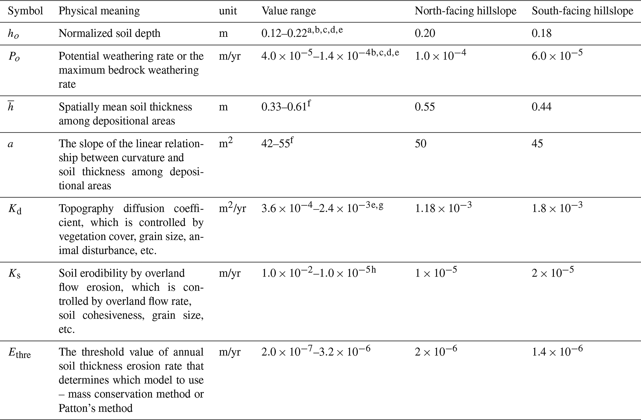
^a We defined h as the distance along the normal direction to the land surface, which gives $e^{-h\cos \mathit{\theta }/h_o}$, where θ is the slope of the land surface in degrees (Pelletier and Rasmussen, 2009). In this case, h_o is adjusted to include cos θ when referring to other literature. ^b Heimsath et al. (1997). ^c Heimsath et al. (2000). ^d Heimsath et al. (2005). ^e Dietrich et al. (1995). ^f Patton et al. (2019). ^g Fernandes and Dietrich (1997). ^h Kilinc and Richardson (1973).

2.1.1 Mass conservation method

The mass conservation equation of soil thickness that combines soil surface transport and soil production processes can be expressed as follows:

$$\begin{array}{}\text{(1)}& {\displaystyle \frac{\partial h}{\partial t}}=P-\mathrm{\nabla }\cdot q_{\mathrm{d}}-\mathrm{\nabla }\cdot q_{\mathrm{s}},\end{array}$$

where h is soil thickness [L], t is time [T], P is soil production rate [L/T], q_d and q_s is the volume flux of sediment transport per unit width resulting from diffusion-driven and overland flow-driven erosion, respectively [L²/T]. The diffusion-driven soil transport rate ∇⋅q_d is the outcome of combining wind erosion, biogenic disturbance, soil creep, and rain drop splash. On steep slopes, the following nonlinear slope-dependent transport law is often used for topographic analysis and numerical experiments and has been successfully demonstrated by field studies and laboratory experiments (Andrews and Bucknam, 1987; Perron, 2011; Roering et al., 1999, 2001):

$$\begin{array}{}\text{(2)}& q_{\mathrm{d}}=-{\displaystyle \frac{K_{\mathrm{d}}\mathrm{\nabla }\mathit{\eta }}{\mathrm{1}-{\left(\mathrm{\nabla }\mathit{\eta }/S_{\mathrm{c}}\right)}^{\mathrm{2}}}},\end{array}$$

where K_d is the diffusion coefficient [$L^{\mathrm{2}}/T$] and S_c=1.25 (Roering et al., 1999) is a critical surface slope. The equation implies that when the slope (∇η) is far less than S_c, the relationship between diffusion flux and slope is almost linear; when the slope approaches S_c, q_d increases rapidly.

The overland flow-driven soil transport rate ∇⋅q_s is expressed as the spatial divergence of stream power (Yan et al., 2019):

$$\begin{array}{}\text{(3a)}& {\displaystyle }\mathrm{\nabla }\cdot q_{\mathrm{s}}={\displaystyle \frac{q_{\mathrm{s},\mathrm{out}}-\mathrm{\Sigma }{q}_{\mathrm{s},\mathrm{in}}}{d_{\mathrm{s}}}},\text{(3b)}& {\displaystyle }{q}_{\mathrm{s}}=K_{\mathrm{s}}{\left(H_{\mathrm{w}}S\right)}^{\mathit{\beta }},\end{array}$$

where K_s is the soil erodibility coefficient [$L^{\mathrm{2}-\mathit{\alpha }}/T$], S is the slope along-flow direction [–], and β is an empirical constant for surface erosion, where β=1.68 (Yan et al., 2019). H_w is surface water depth [L], which is expressed in a 2-D diffusive form (Lal, 1998):

$$\begin{array}{}\text{(4)}& {\displaystyle \frac{\partial H_{\mathrm{w}}}{\partial t}}={\displaystyle \frac{\partial }{\partial x}}\left(D_h{\displaystyle \frac{\partial H_{\mathrm{w}}}{\partial x}}\right)+{\displaystyle \frac{\partial }{\partial y}}\left(D_h{\displaystyle \frac{\partial H_{\mathrm{w}}}{\partial y}}\right),\end{array}$$

where D_h is a diffusion coefficient controlled by water depth, land surface gradient, and Manning's coefficient (Lal, 1998; Yan et al., 2019).

The soil production rate function has been developed to calculate only the development of mobile soil (it excludes the immobile saprolite layer) (Heimsath et al., 1997). The calculation of the soil production rate makes use of two assumptions: (1) production rate exponentially decreases with soil thickness, and (2) production rate has a humped relationship (or a “belly-shape”) along soil depth (Dietrich et al., 1995; Heimsath et al., 2001; Pelletier and Rasmussen, 2009). Because the humped relationship is not yet well validated by field observations, in this study we rely only on the exponential model to represent soil production rate:

$$\begin{array}{}\text{(5)}& P={\displaystyle \frac{{\mathit{\rho }}_r}{{\mathit{\rho }}_{\mathrm{s}}}}{\displaystyle \frac{\mathrm{1}}{\cos \mathit{\theta }}}{P}_o{e}^{-h\cos \mathit{\theta }/h_o},\end{array}$$

where ρ_r and ρ_s are bedrock and soil bulk density, respectively, [$M/L^{\mathrm{3}}$]. The mean value of the soil bulk density at sampling sites is 0.948 [g/cm³], and the bedrock bulk density for weathered shale from our deep samples is estimated to be 1.26 [g/cm³]. P_o [$L/T$] and h_o [L] are empirical constants for soil production, and θ is the slope of the land surface in degree [–] because the direction of soil thickness is perpendicular to the land surface.

Under the assumption of steady-state conditions, which have been observed in several mountainous area studies (Dietrich et al., 1995; Vanwalleghem et al., 2013), we can solve soil thickness from the mass conservation equation. The validity of this assumption for the site studied here will be presented in Sect. 3. By adopting this assumption, the soil thickness (h) can be solved from the mass conservation equation (Eq. 1) as follows:

$$\begin{array}{}\text{(6)}& {\displaystyle \frac{{\mathit{\rho }}_r}{{\mathit{\rho }}_{\mathrm{s}}}}{\displaystyle \frac{\mathrm{1}}{\cos {\mathit{\theta }}_s}}{P}_o{e}^{-h\cos \mathit{\theta }/h_o}-\mathrm{\nabla }\cdot q_{\mathrm{d}}-\mathrm{\nabla }\cdot q_{\mathrm{s}}=\mathrm{0}.\end{array}$$

The soil thickness value h can be directly solved here because ∇⋅q_d and ∇⋅q_s are independent of soil thickness. One issue that arises here is that there is no real number for soil thickness if $\mathrm{\nabla }\cdot q_{\mathrm{d}}+\mathrm{\nabla }\cdot q_{\mathrm{s}}<\mathrm{0}$ where there is a continuous depositing of surface soil. Therefore, we introduce Patton's method (Patton et al., 2018) in depositional areas to overcome this drawback in the following section.

2.1.2 An empirical approach for depositional areas

Based on field measurements among five mountainous watersheds, Patton et al. (2018) found that soil thickness has a linear relationship with curvature:

$$\begin{array}{}\text{(7)}& h=a\mathrm{\nabla }\cdot \mathrm{\nabla }\mathit{\eta }+\stackrel{\mathrm{‾}}{h},\end{array}$$

where $\stackrel{\mathrm{‾}}{h}$ is the spatial mean value of soil thickness and a is a constant value which is determined by having a negative linear relationship with the standard deviation of curvature. In our model, we take a as an independent parameter instead of being calculated based on curvature, which adds one more degree of freedom to the model.

2.1.3 Investigation of the lidar DEM smoothing range for curvature

In the empirical equation (Eq. 7), the curvature (∇⋅∇η) is the only spatial variable that determines the soil thickness. Further, the topographic curvatures are very sensitive to the resolution of the DEM. If the grid size of the DEM is large, then the topography could be over-smoothed, thus underestimating the actual curvature. On the other hand, if the grid size of elevation is small, then there could be temporary pits or burrows in the topography, which can result in large local curvature values that do not represent the soil production processes. To identify a reasonable range of DEM resolution for calculating ∇⋅∇η, we explored three approaches to reproduce the DEM by (1) smoothing the DEM over space, (2) polynomial fitting of the DEM, and (3) smoothing the DEM over time. The smoothed DEM is for calculating curvature in the imperial method only (Eq. 7), and the rest of all other calculations (Eqs. 1–6) still use the original lidar DEM as the input.

Smoothing of the DEM over space is done by replacing the value of a 2-D grid cell with the mean value of its surrounding neighbors. The size of its neighbor cells follows 3Δx (8 neighbors), 5Δx (24 neighbors), 7Δx (48 neighbors), … , (2N+1)Δx (${\left(\mathrm{2}N+\mathrm{1}\right)}^{\mathrm{2}}-\mathrm{1}$ neighbors), respectively, where Δx is the original resolution (i.e., 0.5 m) and N is an integer; following this, a moving window replaces the value of every single 2-D grid cell in the 0.5 m lidar. The polynomial fitting of the DEM is achieved by fitting a second-order polynomial to grid cells within a specified radius and repeating this at each grid cell within the study area. For example, the elevation is fitted by $\mathit{\eta }=a_{\mathrm{1}}{x}^{\mathrm{2}}{y}^{\mathrm{2}}+b_{\mathrm{1}}{x}^{\mathrm{2}}y+b_{\mathrm{2}}x{y}^{\mathrm{2}}+c_{\mathrm{1}}{x}^{\mathrm{2}}+c_{\mathrm{2}}{y}^{\mathrm{2}}+\mathrm{d}xy+e_{\mathrm{1}}x+e_{\mathrm{2}}y+f$, where a₁, b₁b₂c₁, c₂d, e₁, e₂​​​​​​​, and f are parameters to fit the polynomial curve. The curvature value is $\mathrm{\nabla }\cdot \mathrm{\nabla }\mathit{\eta }=\mathrm{2}{c}_{\mathrm{1}}+\mathrm{2}{c}_{\mathrm{2}}$. The DEM smoothing over time is performed by discretizing the diffusion equation $\frac{\partial \mathit{\eta }}{\partial t}=K_{\mathrm{d}}\mathrm{\nabla }\cdot \mathrm{\nabla }\mathit{\eta }$, which gives ${\mathit{\eta }}_n={\mathit{\eta }}_{\mathrm{1}}+\mathrm{\Delta }t\times K_{\mathrm{d}}{\mathrm{\Sigma }}_{i=\mathrm{1}}^{n-\mathrm{1}}\mathrm{\nabla }\cdot \mathrm{\nabla }{\mathit{\eta }}_i$, where subscript i, 1, and n denote the time step. A longer time period (higher n value) results in a smoother topography, so the DEM is smoothed into different levels with different n values. To the authors' knowledge, the smoothing over time approach is new and original in this study.

2.1.4 Combine the mass conservation method with the empirical method

For the mass conservation equation, the steady-state assumption is used for the soil thickness estimation in the assumption that the soil production balances the physical erosion, as used in other studies (Pelletier and Rasmussen, 2009; Pelletier et al., 2016; Dietrich et al., 1995). Therefore, the mass conservation method with the steady-state assumption can be used to solve the soil thickness at erosional sites but has a limitation at depositional sites (Eq. 6, Dietrich et al., 1995). Patton's method is better adapted to depositional sites. However, it can provide negative values of soil thickness at erosional sites where there are zones with high negative-curvature values. In addition, in a low gradient and divergent area, if the soil transport rate is assumed as a linear relationship with curvature (i.e., $\mathrm{\nabla }\cdot q_{\mathrm{d}}=-K_{\mathrm{d}}\mathrm{\nabla }\cdot \mathrm{\nabla }\mathit{\eta }$, and $\mathrm{\nabla }\cdot q_{\mathrm{s}}=\mathrm{0.0}$), then Eq. (6) can be further simplified in that the soil thickness has a natural logarithm relationship with curvature (i.e., $h=-m\times \ln \left(\mathrm{\nabla }\cdot \mathrm{\nabla }\mathit{\eta }\right)+C$, where m and C are constant parameters that can be calibrated from field sampling data. However, Patton's method (Patton et al., 2018) always assumes a linear relationship between soil thickness and curvature. This may be why his empirical relationship does not work very well in the erosional areas. However, this can be compensated for by using the mass conservation method.

We combine the two methods by applying the mass conservation method to most erosional sites and then applying the empirical method to all depositional sites and a potentially small portion of erosional sites where the curvature values are negative but close to zero. The threshold value used to separate these two methods is represented as E_thre [$L/T$] (E_thre≥0):

$$\begin{array}{}\text{(8)}& \left\{\begin{array}{cc}\mathrm{\nabla }\cdot q_{\mathrm{d}}+\mathrm{\nabla }\cdot q_{\mathrm{s}}>E_{\mathrm{thre}},& \text{mass conservation},\\ \mathrm{\nabla }\cdot q_{\mathrm{d}}+\mathrm{\nabla }\cdot q_{\mathrm{s}}\le E_{\mathrm{thre}},& \text{Patton's method},\end{array}\right.\end{array}$$

where the threshold, E_thre, is a condition of the soil erosion rate and equal to or larger than zero value. If $\mathrm{\nabla }\cdot q_{\mathrm{d}}+\mathrm{\nabla }\cdot q_{\mathrm{s}}>E_{\mathrm{thre}}$ at a 2-D grid cell, then this cell must be an erosional site; if $\mathrm{\nabla }\cdot q_{\mathrm{d}}+\mathrm{\nabla }\cdot q_{\mathrm{s}}\le E_{\mathrm{thre}}$, then this cell can be either a depositional site (if $\mathrm{\nabla }\cdot q_{\mathrm{d}}+\mathrm{\nabla }\cdot q_{\mathrm{s}}\le \mathrm{0})$ or a slightly erosional site (if $\mathrm{0}<\mathrm{\nabla }\cdot q_{\mathrm{d}}+\mathrm{\nabla }\cdot q_{\mathrm{s}}\le E_{\mathrm{thre}}$). In most of areas, a divergent topography corresponds to erosional areas and vice versa for depositional areas. However, here we use the transport rate instead of the curvature as the criteria to choose between the two methods because there are possibly sites that are convergent but erosional where overland flow erosion is stronger than the diffusive deposition. In other words, areas where $\mathrm{\nabla }\cdot q_{\mathrm{d}}+\mathrm{\nabla }\cdot q_{\mathrm{s}}\le \mathrm{0}$, it must be a convergent area and undergoing deposition, but if it is a convergent area, it is unnecessary to be $\mathrm{\nabla }\cdot q_{\mathrm{d}}+\mathrm{\nabla }\cdot q_{\mathrm{s}}\le \mathrm{0}$. In addition, we assign E_thre≥0 instead of equal to zero, aiming to provide more flexibility to switch between the two methods. Overall, E_thre is supposed to be very close to zero. We conducted a grid search to calibrate the parameters and discuss the corresponding posterior distribution of parameters in Sect. 4.3.

2.2 Sensitivity analysis of the model parameters

We introduce the Morris one-step-at-a-time (OAT) method for a sensitivity analysis of parameters used in the hybrid model. Given the uncertainty of the input parameters (Table 1), we applied the Morris OAT method to quantify parameter sensitivity (Campolongo et al. 2007; Morris, 1991). The Morris method provides global sensitivity indices over the parameter space at a relatively limited computational cost (Wainwright et al., 2014). With a set of k parameters {x} in that $\left\{x_i|i=\mathrm{1},\mathrm{2},\mathrm{\dots },k\right\}$, the output from the combined model is f(x). The Morris method first generates a randomly assigned set of parameters in a discrete parameter space and then changes one parameter at a time. The (k+1) simulations are required to complete one path, which has one fixed parameter but changes all other parameters. This path is repeated for randomly generated parameter sets, with the total run being r(k+1) where the number of paths is r. By normalizing parameters and uniformly spacing from 0 to 1 with (p−1) intervals, the elementary effect is given as follows:

$$\begin{array}{}\text{(9)}& {\mathrm{EE}}_i={\displaystyle \frac{\mathrm{1}}{\mathit{\tau }}}{\displaystyle \frac{f\left(x_{\mathrm{1}},x_{\mathrm{2}},\mathrm{\dots },x_{i-\mathrm{1}},x_i+\mathrm{\Delta }+x_{i+\mathrm{1}},\mathrm{\dots },x_k\right)-f\left(\mathbf{X}\right)}{\mathrm{\Delta }}},\end{array}$$

where τ is a scaling factor, {x} is a randomly selected parameter set, and the fixed increment $\mathrm{\Delta }=p/\left(\mathrm{2}\left(p-\mathrm{1}\right)\right)$ (Campolongo et al., 2007).

Here, we use iTOUGH2 (Wainwright et al., 2014) to generate sets of parameters. Then we sample r(=20) elementary effects for each parameter. The standard deviation (σ) and absolute of the mean value ($\left|\mathit{\mu }\right|$) of elementary effect of each parameter can be used to investigate the importance and nonlinearity in the combined model. To avoid the influence of non-monotonicity when some effects cancel each other out (Campolongo et al., 2007), we use the absolute mean value instead of the mean value in this study. Our work focuses on the sensitivity of how soil thickness is dictated by landscape characteristics such as the hillslope diffusion coefficient, soil erosion coefficient, and the saprolite-to-soil weathering capacity.

2.3 Random forest regression

In addition to the hybrid modeling approaches, we use a machine-learning approach random forest (Breiman, 2001) to predict the soil thickness for comparison purposes to the hybrid method. The features to train the model are topographic and land cover data obtained from remote sensing. The random forest analysis also helps to identify important predictors for soil thickness. Random forest is capable of averaging the generated regression trees from bootstrapped subsampled data. This algorithm is nonparametric by assuming no specific data distribution ahead of time (Hastie, 2001). We use the “sklearn” Python package for this study.

The random forest algorithm input dataset comprises topographic and land cover features, including aspect, gradient, curvature, topographical flow accumulation, normalized difference vegetation index (NDVI), canopy water content, topographical position index (TPI), etc. (Brodrick et al., 2020; Chadwick et al., 2020; Goulden et al., 2020) at 10 m resolution and smoothing with a moving window at different sizes (e.g., 30, 50, and 90 m) (See Table S1 for the full list of features). Because the field observations have limited sampling points (78), we use the leave-one-out cross-validation method (Efron, 1982) where the number of folds equals the number of instances in the dataset. The random forest algorithm is applied once for each instance, using all other instances as a training set and using the selected instance as a single-item test set.

3 Study site description and data sampling

Our study site is within the East River watershed, which represents a typical headwater mountainous watershed in the upper Colorado River basin in Colorado. The East River watershed is a test bed aiming to improve predictions of hydrology-driven biogeochemical activities. There is a focus on this watershed because it hosts a wide spectrum of vegetation cover and features various hydrologic and geomorphologic processes. It is a headwater to the Colorado River that supplies 1 in 10 Americans with water for municipal usage and irrigation for over 22 000 km² (Hubbard et al., 2018). This ∼126.5 km² watershed has a continental climate with long, cold winters and short, cool summers, with monthly mean temperature ranging from −9.2 to 9.8 ^∘C. The annual precipitation, based on 3 years of monitoring (2015–2018), is between 659 and 750 mm, the majority of which falls as snow, followed by mid- to late-summer monsoonal rainfall.

We consider opposite facing hillslopes to determine whether the variability in meteorological forcing drives differences in the soil thickness (Pelletier et al., 2018). Our study sites (Fig. 1a) include northeast- and southwest-facing hillslopes (for simplicity, referred to as north-facing and south-facing hillslopes) connected to a floodplain (Fig. S2) spanning a total of 0.4 km² and located with an elevation range from ∼2755 to 2922 m at ∼38.93^∘ N latitude and ∼106.95^∘ W longitude. The differences in slope and aspect drive differences in hillslope energy balance, snowmelt timing, and vegetation seasonal dynamics. The south-facing slope shows a thinner snowpack resulting from episodic melt events scattered throughout the winter and spring, whereas the north-facing slope develops a thicker seasonal snowpack that primarily melts during a large snowmelt event occurring over several weeks in spring (Hinckley et al., 2014). Based on the field campaigns in 2019, soils in this area are composed of 15 % sand, 47 % silt, and 38 % clay. Several remote sensing products available at this site were used in this study including 0.5 m lidar DEM and topographic and vegetation features (Table S1).

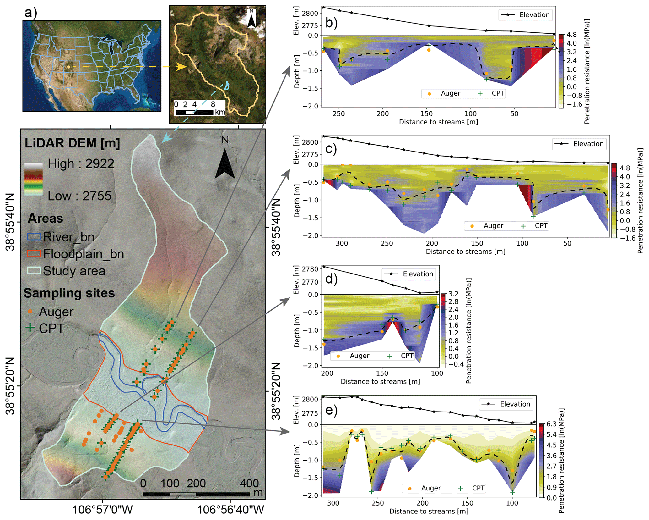
Figure 1 Study site and soil thickness observation. (a) Study site in the East River watershed, CO, USA. The lidar DEM is 0.5 m (Goulden et al., 2020). (b–e) Soil thickness measured by auger (orange dots) and cone penetrometer (CPT) (green cross) data along four transect lines. The CPT data are presented as natural logarithm. The CPT-inferred vertical profiles of resistance values at each surveyed location have been interpolated along the transects by using a kriging method. The dashed lines are estimated soil thickness by averaging the auger and CPT measurements.

The last glacial advance and retreat in the upper Colorado River basin is dated between 16.1 and 20.8 ka (Brugger, 2010). Glacial deposits are mapped at many locations throughout the watershed (Gaskill, 1991; Fig. S3), but they are rather isolated and have a limited spatial extent, including in the area analyzed in this study. A former study at the same site analyzed 40 hand-augured soil cores and showed progressive changes in color and texture among soil, weathered zone, and unweathered bedrock with depth (Wan et al., 2019). Further, among the total of five wells drilled at the site, none of them reported the presence of a glacial deposit (Tokunaga et al., 2019; Wan et al., 2019). It is likely that the glacial legacy scoured the valley to bedrock and that the glacial retreat reset the “clock” for soil formation mostly via in situ bedrock weathering and (to a lesser extent) via colluvial deposition.

Soil thickness was measured at 78 locations across the north- and south-facing slopes. Many studies dig soil pits or use augers to distinguish the contact layer between mobile and immobile regolith layers (Catani et al., 2010; Heimsath et al., 1997; Patton et al., 2018; Pelletier and Rasmussen, 2009). Here, we chose two independent methods to measure the soil thickness of the two hillslopes. We used an auger to drill and sample 78 points within the two hillslopes and used a dynamic cone penetrometer technique (CPT) (Vanags et al., 2004) to measure two transects along each side of the hillslopes, sampling 54 locations in total (Fig. 1a).

At this study site, we used and compared both auger and CPT measurements to estimate soil thickness. The CPT measurements provide a vertical profile of soil resistance for a soil column. We tested the accuracy of the CPT measurement and found that the CPT (i) shows the largest change in resistance when entering weathered bedrock and (ii) can be stopped very sharply only in the presence of a boulder, in which case the resistance is so strong that the measurement was deemed suspicious and repeated nearby. Because the CPT may not clearly identify the potential presence of moraine deposits, we also visually inspected the soil and saprolite materials extracted by the auger. From the auger, the transition zone from soil to the saprolite or bedrock is based on the material size and color of retrieved samples (Fig. S4). When the auger reaches the bedrock shale, it cannot penetrate easily. We believe our measurement is relatively accurate and efficient, which provides a consistent assessment of soil thickness over space in comparison to other existing methods. Figure 1b–e show the relationship between soil thickness estimated from auger, CPT, and local elevation. There is a high variation in soil thickness from local to hillslope scales. To fully take advantage of all the sampling data, we used auger data to fit values for CPT (Fig. S5). The CPT and auger data are mostly in agreement. For soil thicknesses less than ∼0.5 m, the CPT data are slightly higher than the auger, and for soil thickness larger than ∼0.5 m, the CPT data are slightly lower.

4 Results and discussion

In this section, we first investigate the scaling issues from DEM resolution with curvature and then discuss the sensitivity of all the parameters used in this hybrid model. Next, we show both the soil thickness predictions based on the hybrid model with the optimal curvature and the soil thickness results from the random forest machine-learning approach. Finally, we discuss the relationship between soil thickness, surface transport rate, and weathering rate as determined by the hybrid model.

4.1 Model parameterization of curvature with different smoothing techniques of DEM

The topographic curvature is the key variable for estimating the soil thickness for the empirical approach. However, curvature is an inherently resolution-dependent topographic feature that is derived from a DEM. A 0.5 m DEM can provide “noises” for the results of curvature. The goal here is to determine the optimal DEM resolution for curvature to match with the sampling data, and the smoothing methods provided here are only for the calculation of curvature. To investigate the optimal resolution of the DEM for calculating curvature, we tested three approaches as explained in Sect. 2.1.3: smoothing the DEM over space, polynomial fitting of the DEM, and smoothing the DEM over time. For smoothing over space, the elevations of original 0.5 m DEM were replaced by utilizing the mean elevation of the surrounding adjacent cells at the range of 1.5, 2.5, … , and 13.5 m. For the polynomial fitting, the diameter is also chosen over the same range and intervals as the way of smoothing the DEM. For smoothing over time, the evolution period of the topography is taken as 0, 0.25, 0.5, … , 3.25 kyr. We compare the root-mean-square deviation (RMSD) between the sampling results and simulation results of soil thickness as an indicator of the optimal resolution for calculating the curvature (Fig. 2). The sets of parameters used for each spatial or temporal resolution are determined by comparing with the field sampling data, with each parameter increasing linearly from the minimum value to the maximum (the same datasets as in the Morris OAT method). We chose the set of parameters which gives the smallest RMSD.

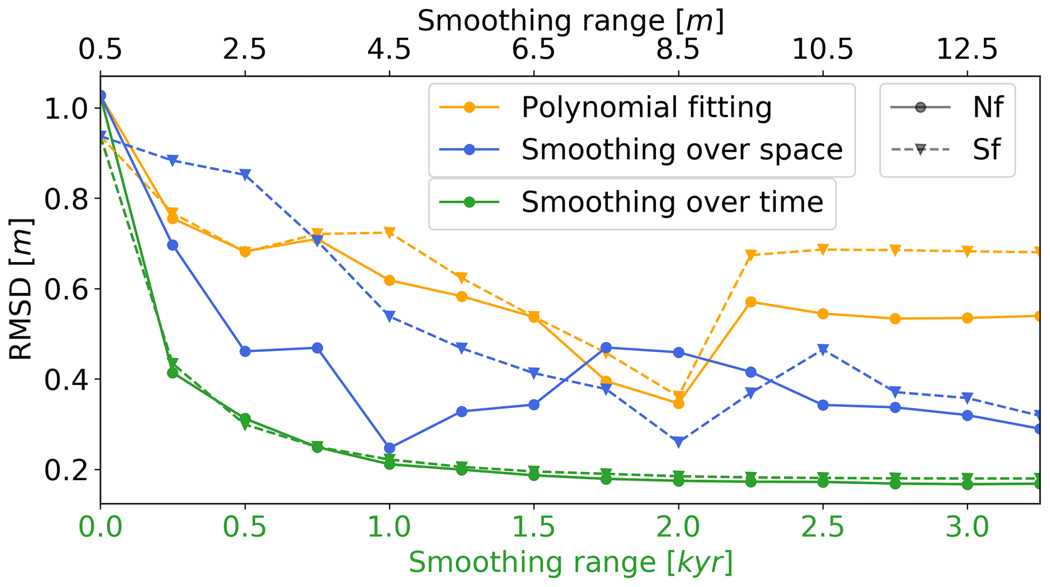
Figure 2 Smoothing techniques to find the best resolutions of DEM for curvature. For the smoothing over time approach, the time step is 1 year; the diffusion coefficient, K_d, is $\mathrm{11}\times {\mathrm{10}}^{-\mathrm{3}}$ m²/yr and $\mathrm{18}\times {\mathrm{10}}^{-\mathrm{3}}$ for the north-facing and south-facing hillslopes, respectively. Nf stands for north-facing hillslope, and Sf stands for south-facing hillslope.

Different smoothing methods and study sites correspond to their own optimal DEM resolution for curvature (Fig. 2). For example, in this study the north-facing hillslope shows the best fitting with 4.5 m DEM smoothing over space, but the south-facing hillslope corresponds to 8.5 m. Other studies that calculate curvature with various spatial smoothing constraints show the highest accuracy in model predictions with smoothing ranging between 3 and 10 m (Patton et al., 2018; Tesfa et al., 2009). The polynomial fitting and smoothing over time show the same best fitting results among the two hillslopes, which is 8.5 m and around 2 kyr, respectively. Overall, smoothing the DEM over time provides the smallest RMSD with a relatively high efficiency compared to the other two approaches. Smoothing over time provides relatively constant and stable results for both hillslopes. Therefore, in this study, we use the DEM smoothed over time at year 2 kyr to calculate curvatures. However, we still use the original lidar DEM for the mechanistic model of soil thickness.

4.2 Global sensitivity analysis

We apply the Morris OAT method to investigate the global sensitivity of the seven parameters (Table 1) in the hybrid model. For each parameter, we calculate the absolute of the mean elementary effect, $\left|\mathit{\mu }\right|$, in that the higher number represents higher importance, and the standard deviation of the elementary effect, σ, which represent the nonlinearity effect or interactions with other parameters (Fig. 3). Each dot represents an evaluation of one parameter at one sampling site. In general, the parameters in the mass conservation model have higher $\left|\mathit{\mu }\right|$ values, meaning that they have a more significant impact on soil thickness than the parameters in the empirical model. The diffusion coefficient, K_d, is the most important factor (high $\left|\mathit{\mu }\right|$ value and high nonlinearity (σ)) and thus should be carefully calibrated. It represents soil diffusive-like processes such as soil creeping and biogenic activities. The normalized soil depth (h_o) is also has a higher $\left|\mathit{\mu }\right|$ value, which suggests that it is a very important factor but more linear than K_d due to its relatively small σ. These factors imply that the diffusive process is the most important transport mechanism for hillslope soil erosion rather than the soil erosion from overland flow on the surface of a soil layer (Dietrich et al., 1995; Nicótina et al., 2011; Roering et al., 1999, 2001). They also imply that the normalized soil depth is the most important parameter for estimating the soil production rate at the bottom of the soil layer. The two parameters from the empirical method, a and $\stackrel{\mathrm{‾}}{h}$, are used for soil depositional areas. The sensitivity of a and $\stackrel{\mathrm{‾}}{h}$ are nearly linear (since σ is close to zero), but when the soil thickness reaches an upper limit (2 m in our model) this causes a nonlinear increase in soil thickness and hence a rapid increase in σ.

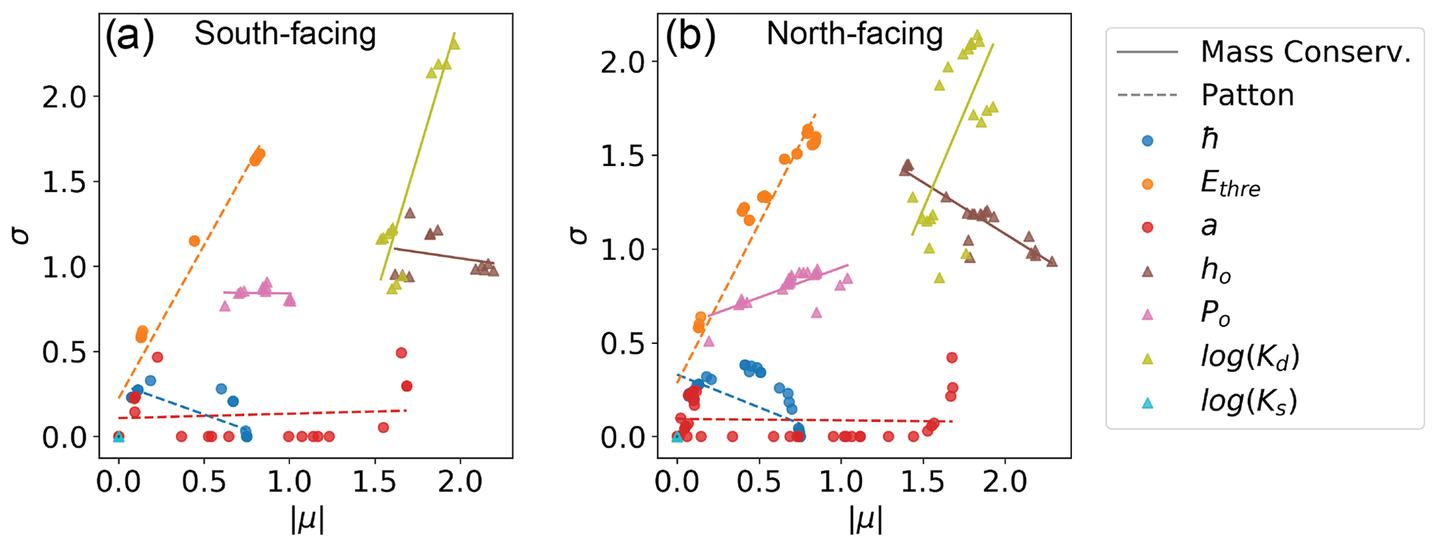
Figure 3 Sensitivity analysis of the seven parameters in the hybrid model. Parameters $\stackrel{\mathrm{‾}}{h}$, E_thre, and a are in Patton's method and h_o, B_p, log (K_d), and log (K_s) are in the mass conservation method. The solid and dashed lines are fitted linear-regression lines to reveal the relationship between the standard deviation (σ) of the elementary effect and the absolute of the mean ($\left|\mathit{\mu }\right|$) of the elementary effect for the mass conservation method and Patton's method, respectively. Each dot is at one sampling location per parameter.

4.3 Hybrid data–model soil thickness predictions and their comparison to measurements

At erosional sites, the erosion from the land surface can be balanced out by the soil formation from the bottom; therefore, the soil thickness may reach a steady-state condition. By coupling soil thickness with landscape evolution, we found that the soil thickness reaches a dynamic steady state after approximately 25 kyr at this study site (Fig. S6), which is consistent with other studies in mountainous areas (Dietrich et al., 1995; Vanwalleghem et al., 2013). This implies that the current soil thickness in the East River watershed may have already reached a steady-state condition since the last glacial legacy. Here, we only focus on the steady-state condition at erosional sites because they are where we apply the mass conservation equation. For depositional sites, the soil gradually accumulates on the land surface; meanwhile, the soil weathers slowly at the bottom. Therefore, the soil thickness is supposed to continuously increase (Dietrich et al., 1995). Due to the complexity of soil depositional environments, such as expansion or compression of soils, we consider using an empirical relationship as appropriate for the soil thickness at depositional areas.

A spatial map of soil thickness that compares modeling predictions and observation results is shown in Fig. 4. In general, the soil thickness of the north-facing hillslopes is greater and has higher variation than that of the south-facing hillslopes. Specifically, soil thickness of the south-facing side ranges from about 0.2 to 1 m, with a mean value of 0.55 m, while on the north-facing side, the soil thickness ranges from 0.15 to 1.5 m, with a mean value of 0.67 m. We use the sampling data from both the auger and the CPT to calibrate the seven parameters (Table 1) for the south-facing and north-facing hillslopes separately. One explanation for the mismatch between modeling and field observations (Fig. 4b) could be that parts of the hillslopes are on terraces. These areas may have fluvial deposits on ancient floodplains before they were turned into terraces (Yan et al., 2018).

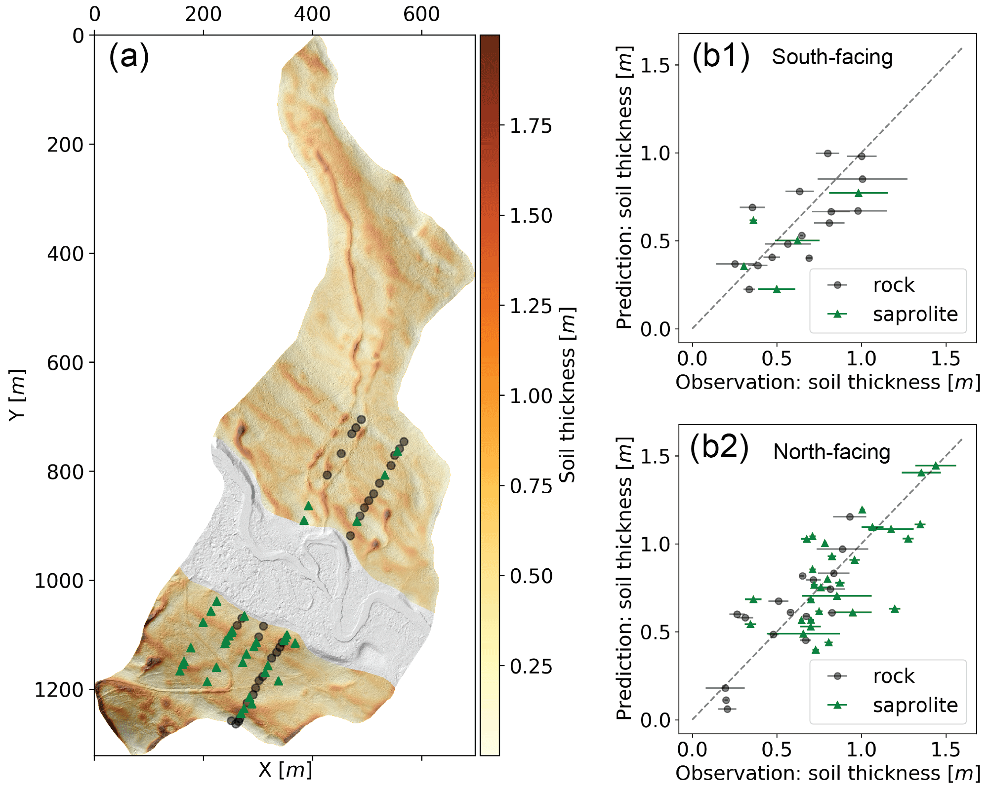
Figure 4 Soil thickness map. (a) Spatial map of soil thickness from modeling. Panels (b1) and (b2) show a comparison between model and field measurements for the south-facing and north-facing hillslopes, respectively. The error bars along the x axis are the differences between auger and CPT data. Gray and green dots present the bottom of the sampling site as bedrock and saprolite, respectively. The correlations, RMSEs, and p values are 0.71, 0.18 m, and $\mathrm{4.2}\times {\mathrm{10}}^{-\mathrm{4}}$ and 0.77, 0.19 m, and $\mathrm{2.32}\times {\mathrm{10}}^{-\mathrm{10}}$ for south-facing and north-facing hillslopes, respectively. Note that the sampling points in the floodplain zone are excluded because our hybrid model aims to predict the soil thickness in hillslopes.

We use the sampling data from auger and the CPT to calibrate the model parameters (Table 1) for the south-facing and north-facing hillslopes separately. The calibration is performed using a grid search approach where the model loops through the entire parameter space with six evenly distributed values for each parameter. The range of each parameter is based on the literature and shown in Table 1. The overland flow coefficient K_s is not included in this process because it is not sensitive to soil thickness (Fig. 3). The ranges of the remaining six parameters are based on the literature and shown in Table 1. We created an ensemble of the soil thickness based on 6⁶(=46646) combinations of parameter sets. We then calculate the root-minimum-square error (RMSE) between the simulated and measured soil thickness across the site. Each set of parameters corresponds to an RMSE, and the distribution of the RMSE as a function of the parameters is shown in Fig. S7. The global minimum can be defined as the set of parameters that provide the lowest RMSE. In this specific study site, we find a unique set of parameters that provide the global minimum with the grid search study. Moreover, when the threshold of RMSE decreases, the number of samples with RMSE below this threshold decrease and converges to the global minimum. This result indicates the absence of other potential strong minima, and we can therefore identify the set of the parameters that provides the global minimum. In addition, we have applied a Bayesian approach to estimate the posterior distribution of parameters, as well as the maximum a posterior estimates (see the Supplement for more information). We find that the maximum a posteriori estimates (Fig. S8) also correspond to the global minimum of the RMSE. Moreover, among the posterior distribution of each parameter, P_o and E_thre are closer to uniform in the south-facing hillslope than the north-facing hillslope. The reason for this may be that the north-facing hillslope has more sampling points, which provides a better estimation than the south-facing hillslope.

The difference in soil thickness between the two hillslopes is evident. This is controlled by insolation due to the topographic aspect. The air temperatures and potential evapotranspiration rates produce significantly different microclimates that determine the structure of different ecosystems and surface process regimes. Weathered shale under the soil layer appears to be mechanically weaker on the north-facing slope because of the thicker saprolite layers (Fig. 4b), which results in less resistance during excavations in the field sampling. This implies that thicker soil depth results from a higher soil water content associated with a longer snowmelt period in the north-facing hillslope. The thicker soil depth in turn provides a higher water storage capability, a higher concentration of fine particles, and more biomass, which leads to a positive feedback (Pelletier et al., 2018; Roering et al., 2010).

4.4 Predictive value of landscape features for estimating soil thickness

We evaluate the correlation between soil thickness from sampling and other landscape features obtained from remote sensing data (Fig. 5). Among about 18 topographic and land cover features with various spatial resolutions, we generated ∼50 topographic matrices (Table S1). The top five topographic matrices, correlating with soil thickness higher than 25 %, from high to low are topographic position index (TPI), curvature, slope degree, topographic wetness index (TWI), and elevation. Other factors such as NDVI (normalized difference vegetation index), leaf mass area, and canopy liquid water do not show obvious correlation with soil thickness. This is consistent with other studies that commonly use the environmental variables such as TWI, elevation, and curvature as the most highly correlated variables in the geostatistical interpolation of soil thickness (Hengl et al., 2004; Kuriakose et al., 2009; Shangguan et al., 2017; Taylor et al., 2013). Among the five highest correlated features, TPI and curvature have the highest correlation (−0.87), which implies that the local relief of ridges and valleys is scalable with the size of the corresponding local curvature.

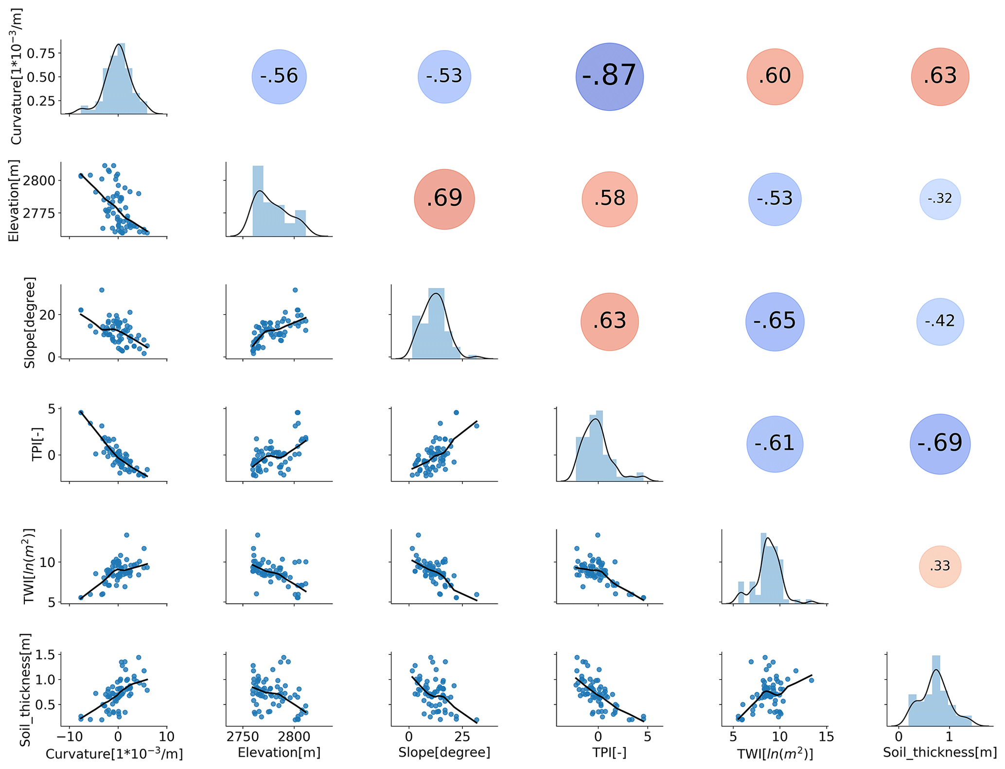
Figure 5 Correlation analysis between soil thickness and the top five most highly correlated topographic features. TPI is 10 m resolution topographic position index, curvature is 10 m resolution curvature, slope is 10 m resolution slope degree, TWI is the 10 m resolution topographic wetness index, and elevation is the 1 m resolution DEM.

Since we have a limited number of soil samples (78), we use the five most highly correlated features as a collection of metrics to perform the random forest modeling. We use the random forest model with leave-one-out cross-validation to predict the soil thickness and compare with the hybrid modeling results (Fig. 6). The result shows that the hybrid model (RMSE = 0.196 m) outperforms the Random Forest model (RMSE = 0.225 m) by ∼13 %. The comparable performance between random forest and the hybrid model suggests that (1) the correlations of soil thickness with topographic metrics are the major driving factors and that (2) the hybrid model is applicable to other sites given similar soil types and topography, without requiring many datasets given the application of process-based laws. To improve the results from machine learning, one may need to collect more data from additional sampling points. However, the advantages of this hybrid model are that there are only seven parameters to calibrate and that fewer sampling points are required. The extension to other watersheds is also easier with the hybrid approach. This hybrid method also provides higher accuracy than Patton's method in this study site, particularly at very thin or thicker soil layers (Fig. S9). Finally, we note that the hybrid modeling approach not only provides the soil thickness distribution but also other outputs from the model, including the surface soil transport and soil production rates, as discussed below.

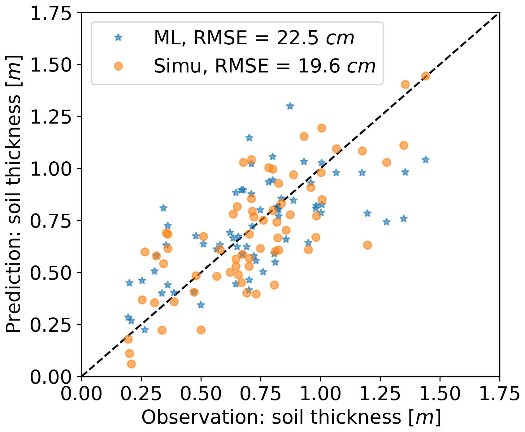
Figure 6 Comparison between observed and predicted soil thickness. Note that ML indicates a machine-learning-based simulation, Simu indicates the hybrid model simulation, and RMSE stands for root-mean-square error.

4.5 Relationship between soil thickness, soil surface transport rates, and soil production rates in two aspects

One of the advantages of this hybrid model compared with machine-learning models is that we can obtain the spatial maps of surface soil transport rates (Fig. 7) and soil production rates (Fig. 8). The probability density functions (PDFs) show that, in general, the south-facing hillslope has a thinner soil thickness and a faster erosion rate than the north-facing hillslope (Fig. 7b). On the south-facing hillslope, where solar radiation is sufficient, soil moisture is a limiting factor that controls vegetation cover in the coupled hydro–bio–geomorphological processes. In contrast, on the north-facing hillslope where solar radiation is limited, the energy becomes a limiting factor of critical zone processes (Pelletier et al., 2018). The higher potential evaporation of south-facing hillslopes results in lower mean soil moisture and thinner vegetation cover, thus triggering feedbacks that result in a higher surface soil erosion rate. Moreover, on the south-facing hillslope, the lower interception of rainfall due to thinner vegetation cover and more sand material from the soil texture (Fig. S10) also increases sediment mobilization by raindrop impacts.

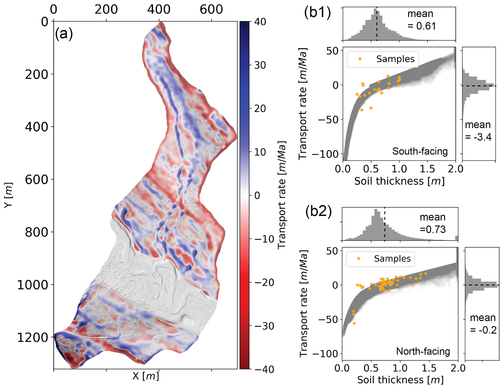
Figure 7 Map of soil surface transport rate. (a) Spatial map of soil transport rate from modeling results. (b1, b2) Relationship between soil thickness and transport rate for the south-facing and north-facing hillslopes, respectively. Positive values of transport rate represent deposition, while negative values represent erosion. The orange dots represent the soil thickness from field measurements.

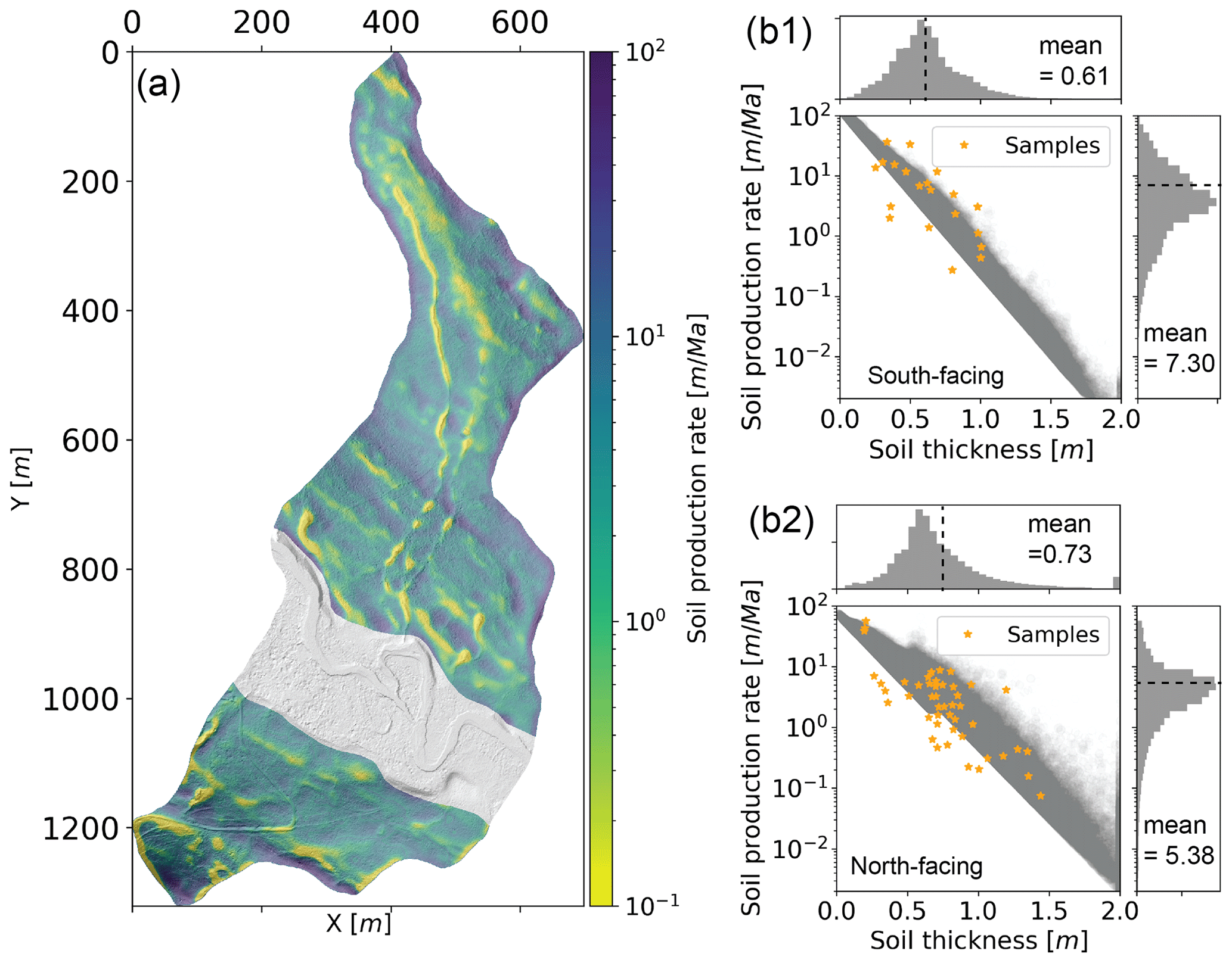
Figure 8 Map of soil production rate. (a) Spatial map of soil bottom (either bedrock or saprolite) production rate from modeling results. (b1, b2) Relationship between soil thickness and natural logarithm of soil production rate for the south-facing and north-facing hillslopes, respectively. The orange dots represent the soil thickness from field measurements.

The contribution of overland flow-driven soil transport (erosion and deposition) to the soil thickness formation is minor compared to the diffusion-driven soil transport. The water depth reaches steady-state after about 6 d with a constant rainfall intensity (i.e., 363 mm/yr) in the study area (Fig. S11a). We apply this spatial map of the water depth to drive the soil transport by overland flow (Eq. 3). The soil transport rate from overland flow mostly happens in the water pathways, which have no ponding after snow melting and storm events. The ratio of the soil transport rate from overland flow to the total soil transport rate is mostly less than 1 % in the two hillslopes (Fig. S11b). This minor impact from overland flow also explains why the parameter K_d is not sensitive in this hybrid model.

The south-facing hillslope corresponds to a higher actual soil production rate than the north-facing hillslope, which is consistent with transport rates in that the south-facing hillslope has a higher erosion rate. One should note that the soil production rate here is different from bedrock weathering rate, which is controlled by water table dynamics (Wan et al., 2019). The actual soil production rate is controlled by the soil thickness and potential production rate, P_o (Eq. 5). A thinner soil layer (south-facing) results in a faster actual soil production rate. A high evapotranspiration and rapid vertical infiltration result in lower P_o. P_o on the south-facing hillslope is slower than the north-facing hillslope (Table 1) due to the microclimate differences between the two hillslopes. On south-facing hillslopes, more of the incoming precipitation is lost to evapotranspiration, which results in less water available for runoff and infiltration (Tran, et al., 2019). In addition, the south-facing slopes experience brief periods of rapid vertical transport following snowmelt events and are drier overall than north-facing slopes (Hinckley et al., 2014).

Pelletier et al. (2013) uses an energy-based variable, effective energy and mass transfer (EEMT), which is a function of precipitation, temperature, and vapor pressure deficit, to quantify the potential rate of bedrock breakdown into soils. Their study also suggests that, under comparable climatic conditions, north-facing hillslopes have a higher EEMT, leading to higher P_o. However, the thicker soil thickness offsets the impact of P_o in that thicker soil thickness results in slower actual soil production rate. This is a possible reason why the north-facing hillslope has slower actual soil production rate even though it has a higher P_o.

5 Conclusion

Soil thickness plays a central role in the feedbacks among surface–subsurface water flow, vegetation, soil production, drainage density, and topography, and these in turn control soil thickness. In this study, we developed a data-driven hybrid model approach to predict the spatial distribution of soil thickness. The hybrid model that we introduced in this study overcomes the drawbacks of both mass conservation laws and empirical relationships. To the authors' knowledge, this is the first study to use a hybrid approach to estimate soil thickness.

Our results show that this hybrid model provides slightly better accuracy than the random forest model (by ∼13 %) on soil thickness estimation. According to both the hybrid and random forest models, soil thickness is more strongly controlled by topographic metrics than vegetational features. The sensitivity analysis of the input parameters (seven in total) show that the diffusion coefficient of hillslope erosion is the most sensitive parameter. We found that smoothing the lidar DEM over time has a higher efficiency than smoothing it over space to obtain the optimal topographic curvature values, which provides the least error between the modeling results and sampling soil thickness.

This hybrid model is a flexible, generally applicable approach to predicting soil thicknesses. The hybrid model, with only seven parameters for calibration, can provide a relatively realistic soil thickness map at other study sites making use of a relatively small number of samples. It can also provide additional output as compared to machine-learning algorithms, including surface soil transport and soil production rates.

Based on field observation and the hybrid model simulation, the north-facing hillslope promotes deeper soil depth than the south-facing hillslope as a result of the different insolation at different aspects. The model analysis suggests that the south-facing hillslope has a slightly faster actual surface transport rate and actual soil production rate than the north-facing hillslope. The potential soil production rate is higher on the north-facing hillslope, caused by relatively dense vegetation cover, less solar radiation, and wetter surface soil material as fundamentally controlled by aspect.

The limitation of the hybrid modeling approach developed here is that it would fail in alluvial depositional sites (i.e., floodplains) where topography is controlled primarily by flooding events (Yan et al., 2018) and strong human intervention landscapes where the surface topography is intensively reshaped for farming and other purposes (Kuriakose et al., 2009; Yan et al., 2020). Integrating process-based modeling, inverse modeling, and statistical analysis provides a thorough understanding of the fundamental mechanisms for soil thickness prediction in hillslopes. Although the example applications in this paper are at two hillslopes, this hybrid model framework should have little limitation when analyzing soil-mantled mountainous hillslopes after calibration with sampling dataset.