the Creative Commons Attribution 4.0 License.
the Creative Commons Attribution 4.0 License.
 | 06 Dec 2021
Multi-objective optimisation of a rock coast evolution model with cosmogenic 10Be analysis for the quantification of long-term cliff retreat rates
Martin D. Hurst
Matthew D. Piggott
Bethany G. Hebditch
Alexander J. Seal
Klaus M. Wilcken
Dylan H. Rood
This paper presents a methodology that uses site-specific topographic and cosmogenic 10Be data to perform multi-objective model optimisation of a coupled coastal evolution and cosmogenic radionuclide production model. Optimal parameter estimation of the coupled model minimises discrepancies between model simulations and measured data to reveal the most likely history of rock coast development. This new capability allows a time series of cliff retreat rates to be quantified for rock coast sites over millennial timescales. Without such methods, long-term cliff retreat cannot be understood well, as historical records only cover the past ∼150 years. This is the first study that has (1) applied a process-based coastal evolution model to quantify long-term cliff retreat rates for real rock coast sites and (2) coupled cosmogenic radionuclide analysis with a process-based model. The Dakota optimisation software toolkit is used as an interface between the coupled coastal evolution and cosmogenic radionuclide production model and optimisation libraries. This framework enables future applications of datasets associated with a range of rock coast settings to be explored. Process-based coastal evolution models simplify erosional processes and, as a result, often have equifinality properties, for example that similar topography develops via different evolutionary trajectories. Our results show that coupling modelled topography with modelled 10Be concentrations can reduce equifinality in model outputs. Furthermore, our results reveal that multi-objective optimisation is essential in limiting model equifinality caused by parameter correlation to constrain best-fit model results for real-world sites. Results from two UK sites indicate that the rates of cliff retreat over millennial timescales are primarily driven by the rates of relative sea level rise. These findings provide strong motivation for further studies that investigate the effect of past and future relative sea level rise on cliff retreat at other rock coast sites globally.
- Article
(9795 KB) - Full-text XML
-
Supplement
(1739 KB) - BibTeX
- EndNote


Fundamental features of a rock coast are a sea cliff and shore platform, and the rate of cliff retreat is foremost the collective result of processes eroding the cliff face horizontally and the shore platform vertically (Sunamura, 1992; Trenhaile, 2008a). The ability to erode a cliff face depends fundamentally on the type of cliff material exposed to the delivery of energy to the cliff surface, usually in the form of waves. In turn, delivery of wave energy is mediated by the configuration of the shore platform, beach width, and wave climate (Sunamura, 1992). Thus, the processes that effect the weathering, erosion, and transport of shore platform, intact cliff, failed cliff, and other beach material are an important part of the whole process of “cliff erosion” (Coombes, 2014; Hurst et al., 2016; Limber and Murray, 2011; Masteller et al., 2020; Naylor and Stephenson, 2010; Prémaillon et al., 2018; Thompson et al., 2019). These complex and varied processes make predicting long-term cliff erosion rates difficult. Erosional processes are governed by climate, relative sea level (RSL), tides, and local lithology type and structure (Kennedy et al., 2014), which further complicate the prediction of large-spatial- and temporal-scale erosion rates at rock coast sites. With climate change threatening the stability of these coastlines through RSL rise and increased storminess (Trenhaile, 2014), accurate long-term predictions of erosion rates will be highly valuable in the development of scenarios within the context of coastal management.
Understanding and quantifying the long-term trajectory of cliff erosion is central to the development of predictive coastal evolution models that account for a changing climate. Current records of cliff retreat can only be observed through historical records, which are typically over an approximately 150-year time period (Brooks and Spencer, 2010; Dornbusch et al., 2008). This time period is monopolised by engineering and modification of coastlines, hindering observations of their natural behaviours (Hurst et al., 2016). Furthermore, infrequent mass-wasting events can obscure relationships between climate and average erosion rates in short-term records (Trenhaile, 2014). This means projections of cliff retreat derived solely from short-term data records can be unreliable (Sunamura, 2015). It is critical that cliff retreat is studied over millennial timescales that are able to integrate changes in RSL rise, the return period of episodic erosion events and that precede the influence of anthropogenic modifications to the coastline.
The contribution of cosmogenic radionuclide (CRN) analysis to the advances in rock coast science is well-known, but further potential in its application to rock coasts is recognised (Trenhaile, 2018). The quantification of rock coast evolution is impeded by scarce and slow erosion indicators and a lack of dateable deposits (Trenhaile, 2008a). However, CRN analysis can be applied directly to the shore platform surface to calculate exposure time and erosion rates (Regard et al., 2012). Cosmic rays interact with target elements in the upper few metres of the Earth's surface to produce CRNs (Gosse and Phillips, 2001). Model predictions of CRN concentrations across a shore platform display a characteristic “humped” distribution profile across-shore (Hurst et al., 2017), for which the magnitude of the hump is inversely proportional to cliff retreat rate (Regard et al., 2012). Previous applications of CRN measurements to cliffs and shore platforms have been used to quantify cliff retreat rates (Duguet et al., 2021; Hurst et al., 2016; Regard et al., 2012; Rogers et al., 2012; Swirad et al., 2020), understand Quaternary-scale shore platform exposure history (Choi et al., 2012), date major mass-wasting events (Barlow et al., 2016; Recorbet et al., 2010), and constrain shore platform denudation rates (Raimbault et al., 2018). Combining CRN analysis with a coastal evolution model can help reveal site-specific, long-term cliff retreat and shore platform lowering rates (Trenhaile, 2018).
A novel contribution here is the use of a morphodynamic model of rock coast development to interpret CRN concentrations. Furthermore, this study is the first application of a morphodynamic rock coast evolution model to real-world sites in order to model past cliff retreat rates. Coupling CRN concentrations with topography can help constrain modelled morphodynamics and replicate real-world sites. Equally, accurate morphodynamic development provided by the coastal evolution model is needed in order to interpret CRN concentrations. Application of a process-based model allows for replication of CRN production through time that corresponds directly to rock coast profile development. In order to apply a morphodynamic model to a real rock coast site and accurately model CRN concentrations, we need a rigorous method of comparing model results with measured field data. Primarily, we need to establish whether the model is capable of replicating both the measured topography and CRN concentrations simultaneously to ensure the modelled cliff retreat rates are an accurate reflection of the evolutionary history at the rock coast sites in question.
In order to interpret CRN concentrations, a process-based model of rock coast development is required. Matsumoto et al. (2016) present an effective exploratory coastal evolution model that simplifies wave properties. The model can produce a wide range of endmember across-shore profile shapes and generally identify dominant erosion processes (Matsumoto et al., 2018). However, simplified processes and lack of field data calibration inhibit the application to real-world sites. As such, replication of an observed topographic profile of a cliff and shore platform has not yet been achieved. Equifinality is often an unavoidable property of modelled geomorphic systems and, as a result of simplified processes, causes the same endmember results to be produced from non-distinctive parameter values. Previous explorations into the relative contributions of wave and weathering-driven erosion revealed evidence of equifinality in the model (Matsumoto et al., 2018). In particular, similar profile shapes were produced in mega-tidal settings when considering a significant range of wave force. The addition of modelled CRN concentrations to the topographic profiles has the potential to address equifinal model results. Moreover, field data calibration can be used to identify and constrain the conditions that cause equifinality so that this abstract model can be applied to real-world sites.
This study uses multiple site-specific datasets in order to calibrate a model that couples the Matsumoto et al. (2016) coastal evolution model and the Hurst et al. (2017) dynamic coastal evolution and cosmogenic radionuclide production model. We use Dakota optimisation software (Adams et al., 2019) with the QUESO Bayesian calibration library (Estacio-Hiroms et al., 2016) to implement multi-objective model optimisation using the Metropolis–Hastings Markov chain Monte Carlo (MCMC) method (Hastings, 1970; Metropolis et al., 1953). We demonstrate that with our optimisation method, wave and weathering processes are adequately simulated so as to model real-world sites. The model was calibrated to a high-resolution, across-shore topographic profile and, more importantly, high-precision 10Be concentrations. We are therefore able to extract further information from the model, such as (1) the antiquity of the shore platform, (2) a time series of long-term cliff retreat rates, and (3) the ability to distinguish between different forms of erosion acting on real-world profiles over a large temporal scale, while addressing and limiting model equifinality. This new capability allows us to better constrain the geomorphic history of rock coast evolution and input model parameters. As a result, the constrained model parameters can be used together with future RSL predictions to project rock coast profile development so that predictions of future coastal erosion rates are possible.
We utilise field datasets taken from two UK sites to develop an approach to calibrate the coastal evolution model (Fig. 1). The first study site at Bideford is located on Devon's north coast in south-west England. The study was carried out within the Bideford Formation, part of the upper Carboniferous deposits of the Culm Basin in Devon, which is composed of nine coarsening-upwards cycles from black mudstone to massive sandstones (Edmonds et al., 1979). The beds are well-exposed in the cliff and platform, are steeply dipping (60–65∘) to the SW, and strike SE–NW roughly perpendicular to the coastline. The intertidal shore platform has a width of ∼230 m and a nearly continuous gradient (tan β) of 0.02. Cliff height reaches 36 m, with a ∼24 m wide beach overlying the cliff–platform junction. The south-west coast of the UK is mega-tidal, with a mean spring tidal range of 8.41 m at the Bideford coastline (National Tidal and Sea Level Facility, 2021).
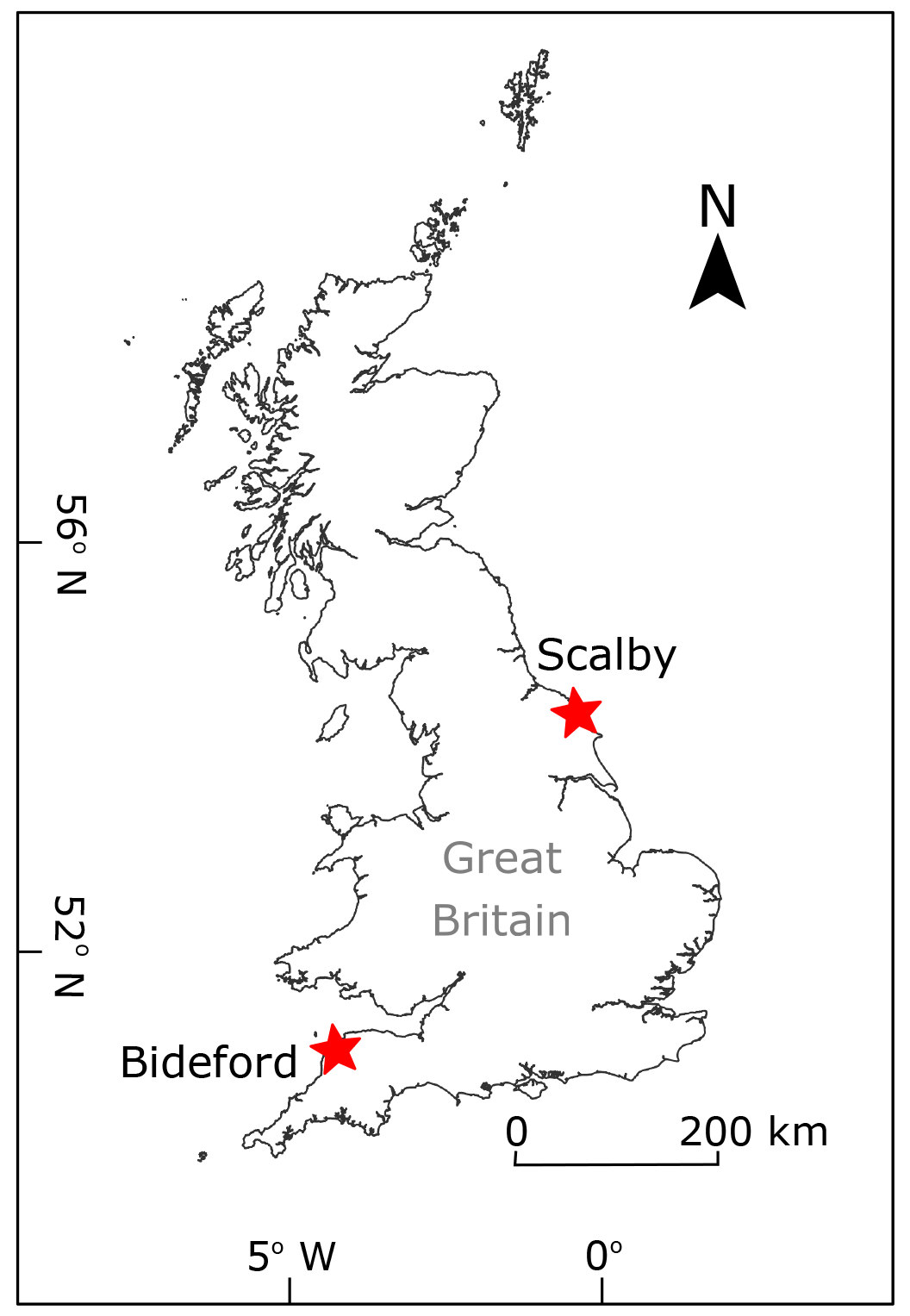
Figure 1Map of Great Britain with two rock coast sites labelled. Bideford is located in south-west England on the north coast of Devon. Scalby is located on the east coast of England in north Yorkshire.
The second study site at Scalby is located in north Yorkshire on the east coast of the UK. The Scalby site is located within the mid-Jurassic Long Nab member of the Scalby Formation, which is comprised of fine-grained sandstone (Riding and Wright, 1989). The beds at Scalby are shallowly dipping (∼12∘) to the SE and strike SW–NE. At Scalby, the intertidal shore platform width reaches ∼240 m and has a gently sloping gradient (tan β) of 0.01, and a steeply sloping 50–80 m high coastal bluff is present. The east coast of the UK has a meso-macrotidal range half of that at the south-west site, with a mean spring tidal range of 4.6 m at the Scalby coastline (National Tidal and Sea Level Facility, 2021).
Using methods described below, we aim to quantify long-term, transient cliff retreat rates that will enable better predictions of erosion rates at rock coast sites across the UK and worldwide. This flexible optimisation method implemented within the Dakota environment allows for simple replication with new datasets and can be applied to a range of rock coast settings.
3.1 Field datasets
Two distinct datasets are used to calibrate the coastal evolution model. The first dataset is an across-shore topographic profile (Fig. 2a). The profile is extracted from a high-resolution digital surface model (DSM) generated by structure-from-motion analysis of aerial photographs collected by an unmanned aerial vehicle (UAV) survey at both sites. The second dataset is a 10Be concentration across-shore profile (Fig. 2b). In situ bedrock samples for CRN analysis were taken along an across-shore transect at ∼10 m intervals from a sandstone bed at both sites. Quartz purification and 10Be isotope dilution chemistry preparation were conducted in the CosmIC laboratory at Imperial College London. Analyses of 10Be9Be ratios using accelerator mass spectrometry (AMS) were carried out at the Australian Nuclear Science and Technology Organisation using the 6 MV Sirius tandem accelerator (Wilcken et al., 2017). Measured 10Be concentrations were normalised to the KN-5-3 standard with an assumed ratio of ( Ma; Nishiizumi et al., 2007). Details of CRN sample collection and preparation, as well as drone survey data collection, processing, and swath profile generation will be presented and interpreted in detail in future work. In this study, our measured data serve solely as input test datasets for developing appropriate multi-objective optimisation routines; thus, details of these test datasets are not central to this investigation.
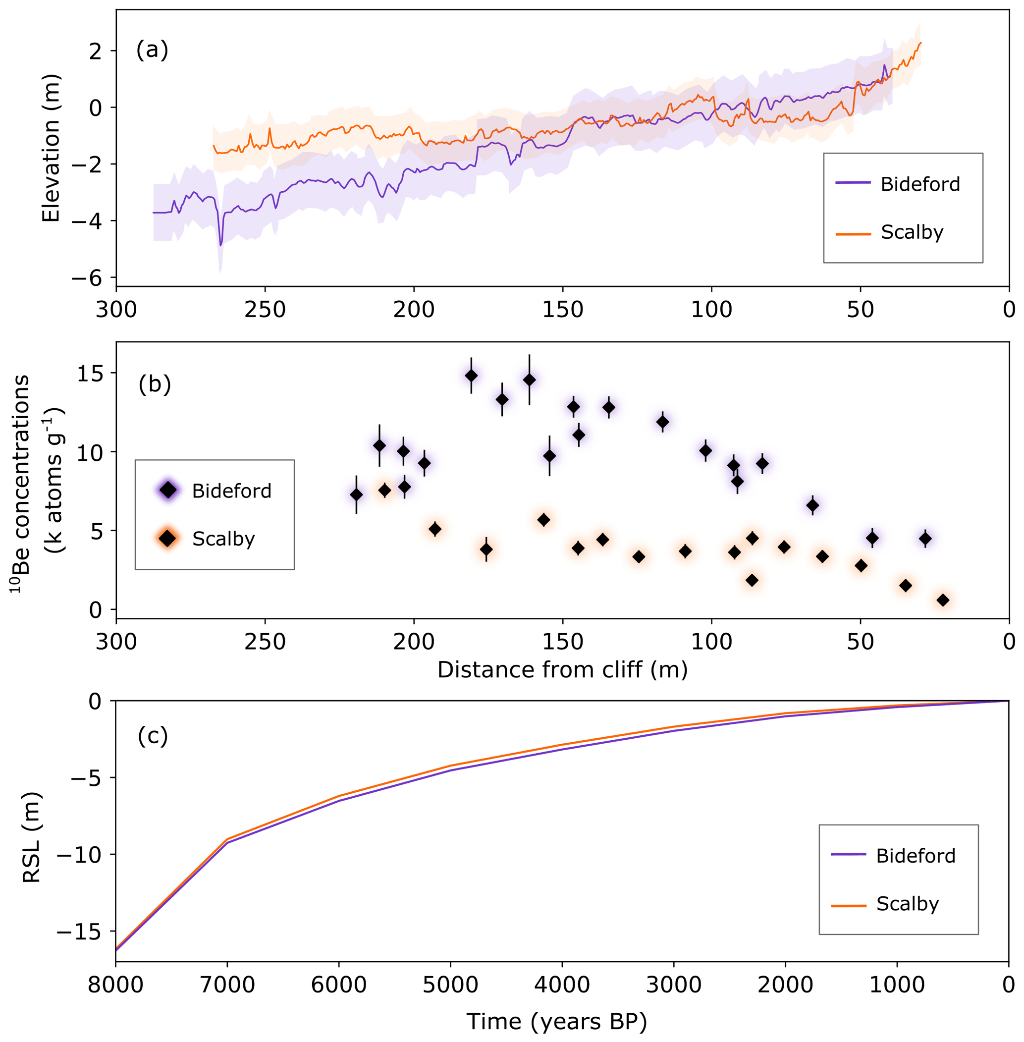
Figure 2Measured topographic profile (a) and 10Be concentration data (b) from the Bideford and Scalby shore platform rock coast sites. Average elevation in the swath profile is shown by the solid line, and uncertainty for the topographic profile shown by the shaded area is the sum of the standard error from a linear regression of the topographic swath profile and the estimated spatial accuracy of the UAV imagery (a). 10Be concentration values (b) are corrected for chemistry background using process blank samples and inherited 10Be using shielded sea cave or cliff samples. Errors are propagated in quadrature, allowing for calculation of corrected 10Be concentrations (see Sect. 3.1). An RSL curve of absolute RSL elevations taken from a GIA model (Bradley et al., 2011) is shown from 8000 years BP to the present day (c).
Measured 10Be concentrations are corrected for both chemistry background and inherited levels of 10Be by subtracting the concentration of 10Be present in process blank samples and a shielded sample taken from a sea cave or cliff base, respectively. Two key 10Be production pathways exist: 10Be produced from spallation reactions (4.0 normalised to sea level high latitude – SLHL) and muogenically produced 10Be (0.028 SLHL). 10Be production in the upper few metres of the Earth surface is dominated by exposure to secondary cosmic-ray neutrons (spallation), whereas muon-produced 10Be prevails with greater depth below the Earth's surface owing to its longer attenuation length (42 000 kg m−2) in contrast to the spallation attenuation rate of 1600 kg m−2 (Braucher et al., 2013). The production of in situ 10Be declines exponentially with depth below the Earth's surface as cosmic-ray flux attenuates (Balco et al., 2008; Gosse and Phillips, 2001; Hurst et al., 2017; Mudd et al., 2016). Because the cliff–sea cave samples are previously shielded by ∼40–80 m of rock (see Sect. 2), the concentration of 10Be within the shielded sample is assumed to be entirely produced from deep-penetrating muons, with no contributions attributed to neutron spallation through exposure to cosmic rays. Correcting shore platform samples using the shielded samples corrects for any 10Be present in the rock before spallogenic 10Be becomes dominant. The exposure time is then calculated from the corrected 10Be concentrations. See Tables S1 and S2 in the Supplement for 10Be concentrations used as model inputs for the Bideford and Scalby sites.
An RSL history record from a glacial isostatic adjustment (GIA) model (Bradley et al., 2011) shows a constant but declining rate of RSL rise across the Holocene for both sites (Fig. 2c). At both sites, the RSL 8000 years BP was at an elevation of ∼16 m lower than the present-day RSL. At Scalby, average rates of RSL rise were reduced from +7.0 to +0.5 mm yr−1 across the last 8000 years. Similarly, at Bideford, average rates of RSL rise were reduced from +7.0 to +0.4 mm yr−1 across the last 8000 years.
3.2 The coastal evolution model
Our model combines a rocky profile model (RPM) for rock coast evolution (Matsumoto et al., 2016) with a rock coast cosmogenic radionuclide production model (Hurst et al., 2017). This coupled model applies a dynamic form of coastal evolution, in which cliff retreat rate is controlled by competing cliff–platform dynamics. Generally, an initial period of rapid cliff retreat results in widening of the shore platform. As a result, increased wave energy dissipation allows less wave energy to reach the cliff base, and cliff retreat rate declines under stable RSL conditions (Hurst et al., 2017; Trenhaile, 2000; Walkden and Hall, 2005). Either platform lowering or RSL rise can maintain energy supply to the cliffs. As a result, platform morphology is an emergent element of the model.
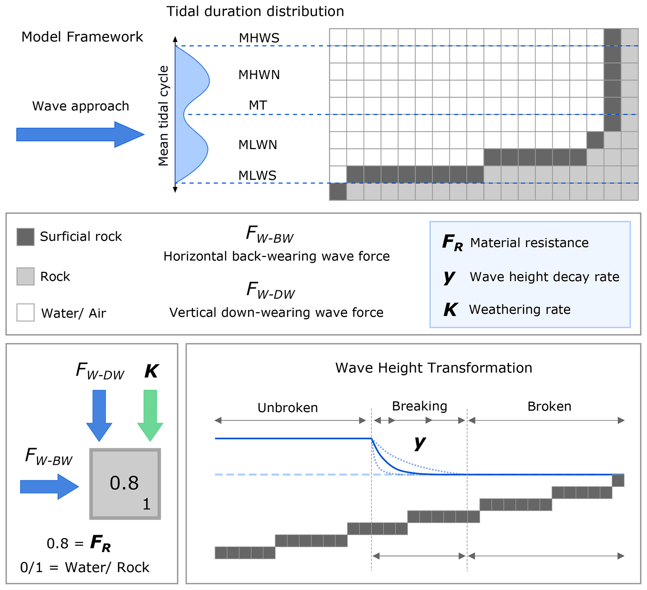
Figure 3Coastal evolution model schematic. Topographic profile cross section constructed in a gridded framework, showing wave approach and influence of tidal duration distribution. MHWS, MHWN, MT, MLWN, and MLWS denote mean high water spring, mean high water neap, mid tide, mean low water neap, and mean low water spring. Binary values of 0 and 1 are assigned to water–air and rock categorised cells, respectively. Rock cells (value 1) are eroded and removed from the profile (assigned value 0) once wave force exceeds material resistance (FW≥FR) (b, c). Subaerial weathering (K) can also lower the material resistance value (FR). Wave height decay rate (y) controls the distance waves can break across the shore platform and, as a result, the erosional potential of wave assailing force FW.
The exploratory model uses a grid framework, in which cells are assigned a binary value of 1 (rock) or 0 (water–air), and represents a cross section transect taken perpendicular to the cliff line (Fig. 3). Wave erosion is considered an erosion-driving process and follows established conceptual rocky shore evolution models, which express wave hydraulic and mechanical properties as wave assailing force and considers both horizontal cliff back-wearing and vertical platform lowering (Payo et al., 2015; Sunamura, 1992; Trenhaile, 2008a) (Fig. 3). Offshore wave height remains fixed throughout a model simulation time; waves are transformed inshore into shallow water and break when wave height exceeds 0.8× water depth. Wave height then decays exponentially across the shore platform after wave breaking is initiated. Erosion achieved by breaking and broken waves can be changed by varying the distance across the shore platform that waves can dissipate energy: wave height decay rate (y) (Fig. 3). A small value for y means wave height will decay slowly, in which case breaking waves exert energy across a greater distance of the shore platform surface, which achieves more erosion. In contrast, a large value for y indicates that wave height will decay quickly and wave-driven erosion covers a shorter distance across the shore platform.
In the model array, each rock cell of the cliff–platform profile is assigned a value for material resistance. The rock cell is eroded and removed from the array (cell values change from 1 to 0) once wave assailing force (FW) exceeds the material resistance value (FR): FW≥FR (Matsumoto et al., 2016) (Fig. 3). The conceptual value for material resistance (FR) is highly simplified by incorporating mechanical, geological, and structural rock factors into a single value to represent rock mass strength (Matsumoto et al., 2016).
Subaerial weathering of the platform's intertidal zone acts to lower the resistance of the rock material (Matsumoto et al., 2016). The distribution of intertidal weathering efficacy is informed by empirical experiments of cyclical wetting and drying (Porter et al., 2010). Maximum weathering rate (K) occurs at the mean high water neap tidal level (MHWN), which is defined by a weathering efficacy distribution (Porter et al., 2010) (Fig. 3). An annual tidal duration distribution (Trenhaile, 2000) is used as an erosion-modulating process by estimating the total annual wave assailing force at each intertidal level (Matsumoto et al., 2016) (Fig. 3).
Cosmogenic radionuclide production is incorporated into the model by coupling a numerical model of 10Be accumulation on eroding shore platforms (Hurst et al., 2017). The concentration of 10Be is calculated for each rock cell at every annual time step. Both 10Be produced from exposure to neutron spallation at the surface and muon-produced 10Be at depth are modelled (see Sect. 3.1). Modelling both production pathways for the surface material and at depth below the shore platform surface is important because both horizontal erosion and vertical erosion of the cliff and shore platform are simulated. Horizontal erosion at the cliff base causes cliff retreat and exposes new shore platform material to spallogenic 10Be production and accumulation. Concentrations of 10Be will increase offshore from the cliff base as exposure times increase. Erosion across the intertidal shore platform, including by platform lowering and intertidal weathering, removes the most abundant 10Be-laden rocks and uncovers rocks with less abundant 10Be underneath. Incoming cosmic rays are shielded from the shore platform by water coverage across the platform surface, which is further influenced by tides and RSL change. As water depth increases offshore, the cosmic-ray flux attenuates exponentially and production in the shore platform surface is reduced (Hurst et al., 2017; Regard et al., 2012). Topographic shielding from the presence of a sea cliff also modulates 10Be production close to the cliff base (Hurst et al., 2017). The combination of scaling factors to account for each of these variables, i.e. production of 10Be in rock, topographic shielding, and water shielding, results in the predicted across-shore humped 10Be concentration profile (Regard et al., 2012).
3.2.1 Model implementation
Other fixed model parameters and initial model conditions are set to the same values as used by Matsumoto et al. (2018) (Table S7 in the Supplement). Once the model burn-in period has been exceeded (first ∼1000 years), the initial conditions, such as platform gradient, have a negligible effect on final outputs of topography, 10Be concentrations, and retreat rates. The RSL history input is taken from the GIA model of Bradley et al. (2011). RSL uncertainty was not considered as we expect it to make little difference to final results. For southern UK sites across the late Holocene, the misfits between measured RSL data and GIA model predictions are minor (Bradley et al., 2011). Uncertainties of magnitude ±0.01–0.1 mm yr−1 of RSL rise have a negligible impact due to the spatial and temporal resolution considered for the model. A fixed mean spring tidal range of 8.41 m for Bideford and 4.6 m for Scalby are used, which are based on tide gauge records (National Tidal and Sea Level Facility, 2021).
We chose to implement a model simulation time of 8000 years. A simulation time of 8000 years BP to the present day captures the RSL history curve for both sites (Fig. 2) with a rapid RSL rise occurring for the first ∼1000 years, followed by a slow decline from 7000 years BP to the present day. Therefore, we can observe how cliff retreat rates will respond to these different stages in the RSL history. Implementing a simulation time of 10 000 years, for example, would show no change to final model outputs but would increase the computer run time unnecessarily. Furthermore, previous studies show that under static RSL conditions, a steady-state equilibrium is reached by 8000 years, in which cliff retreat rates stabilise after rapid initial retreat (e.g. Walkden and Hall, 2005). Modelling rock coast evolution across an 8000-year window means only a Holocene history for shore platform formation has been considered with no possible re-occupation from a previous interglacial period (e.g. Choi et al., 2012). The 10Be concentration datasets used to develop our optimisation routine at both sites exhibit low concentrations, suggesting these rock coast features are formed during the Holocene (Regard et al., 2012). Therefore, these datasets are suitable for modelling Holocene-formed shore platforms as a means to develop this optimisation routine. During the 8000-year simulation time, the topographic profile and 10Be concentrations are calculated and output every year (1-year time step). The model space is split into 10×10 cm gridded cells (Fig. 3).
3.3 Model optimisation
3.3.1 Dakota and multi-objective optimisation
We use Sandia National Laboratory's Dakota optimisation software toolkit (Adams et al., 2019) to implement multi-objective optimisation. The optimisation software was chosen to work with the model because of Dakota's flexibility, ease of testing a variety of methods, and available functionality within the software. In particular, the QUESO Bayesian calibration library (Estacio-Hiroms et al., 2016) is used to apply the Metropolis–Hastings MCMC algorithm. Multiple MCMC simulations are performed, each with different weightings assigned to the topographic profile and 10Be concentration profile to construct a Pareto front of optimised results (see Sect. 3.3.3).
3.3.2 Objective function definition, scaling, and weighting
In this study, we use the coupled model to simulate both a topographic profile and a 10Be concentration profile. The first model output is the cliff–platform profile, which displays a cross section of the elevation, width, and gradient of the modelled shore platform in an across-shore orientation. The second model output is an across-shore 10Be concentration profile. In order for the model to replicate the topography and 10Be concentrations of a real rock coast site, we need to calibrate model results to measured datasets. Our model calibration targets a set of model input parameters that best match the measured data by minimising an objective function (Barnhart et al., 2020). Selected input model free parameters are varied repeatedly within a set parameter space, and model outputs are compared to corresponding data with the aim of minimising residuals between modelled and measured profiles. Because two outputs are generated with the model, we have two objective functions to minimise simultaneously. Multi-objective optimisation is used to find a set of model input parameters that minimises both topographic and 10Be concentration residuals with different weights.
First, the root mean square error (RMSE) is calculated between the modelled and measured DSM-extracted topographic profile and also between the modelled and measured 10Be concentration profile. Modelled outputs and measured data are shifted to the final (present-day) modelled cliff position, with the final cliff position at 0 m. Interpolation is used to assign corresponding modelled data (cell resolution=0.1 m) to every measured data position across the shore profile. For every measured data point, the elevation and concentration residuals are calculated and combined into an RMSE score for both topographic and 10Be concentration model outputs:
In Eq. (1), for each objective function i, the residuals () are calculated between the modelled and measured data values, which are indexed by subscript j. The number of measured data points is distinct to the topographic profile and 10Be concentration profile datasets, and they are denoted by Nj.
Next, both RMSE values are then scaled (si) within Dakota to (1) equalise the magnitude ranges of both the topographic and cosmogenic radionuclide RMSE scores and (2) to set the RMSE magnitudes to a sensible multiple relative to the default measurement error used by Dakota in the likelihood function: variance is assumed to be 1.0 when no measurement error is specified. In this case, we have not considered individual data-point measurement errors in the RMSE calculation. As a result, scaled RMSE scores for both the topographic and 10Be concentration profiles are within the range of ∼0 to 10. Individual weightings (wi) are applied to the scaled RMSE functions for both the topographic and 10Be concentration profiles (Adams et al., 2019). Finally, the scaled and weighted RMSE scores are combined within a Gaussian likelihood function, and the final composite objective function, Likelihoodp, becomes
In Eq. (2), Ni is the number of individual objective functions we aim to collectively minimise. In this case, we have two individual objective functions (Ni=2): a topographic profile and a 10Be concentration profile. Future applications may add additional objective functions (Ni>2): for example, a second CRN concentration profile (e.g. 26Al or 14C). Weightings applied to the separate RMSE scores are denoted by wi, where subscript i refers to specific values associated with each individual objective function. The weightings applied to the topographic profile and 10Be concentration profile are changed between MCMC inversion calculations in order to construct the Pareto set of optimised results (see Sect. 3.3.3). The scaling values are denoted by si and are exclusive to the individual objective function. A topographic profile scaling value is calculated by summing the standard error from a linear regression of the topographic profile and the estimated spatial accuracy of the UAV imagery. The average measurement error of 10Be concentrations for each site is used as a scaling value for the 10Be profile. Table S7 summarises the objective function scaling values for both sites. Subscript p refers to the different set of weights (wi,p) assigned to each objective function (RMSEi) used to construct the Pareto front.
3.3.3 Pareto front results
When performing multi-objective optimisation rather than a single optimal solution, there are multiple optimised solutions, which map out what is known as a Pareto front. We need to consider best-fit model results across a spectrum of objective function combinations because changing the weightings applied to each objective function may result in different best-fit input model parameters. The Pareto front is a set of optimised results for which no improvement can be made to an individual objective function without compromising the performance of at least one of the other objective functions. This set of results is the most optimal set of input model parameters. The Pareto front is constructed by performing numerous MCMC inversions with various weightings given to the RMSE scores that are calculated for the topographic and 10Be concentration profiles for each run. The weighted RMSE values are combined in a likelihood function to form a single-objective function (Eq. 2). In this investigation, a total of five MCMC calculations for each site are performed. For each of the five MCMC runs, the weightings assigned to the topographic and 10Be concentration profile RMSE scores are changed. Weightings assigned to each individual objective function for each MCMC analysis are shown in Table 1. Figure 4 shows a basic framework of the multi-objective optimisation of the coupled model.
Table 1Weightings assigned to the topographic and 10Be concentration RMSE scores for the five MCMC calculations.
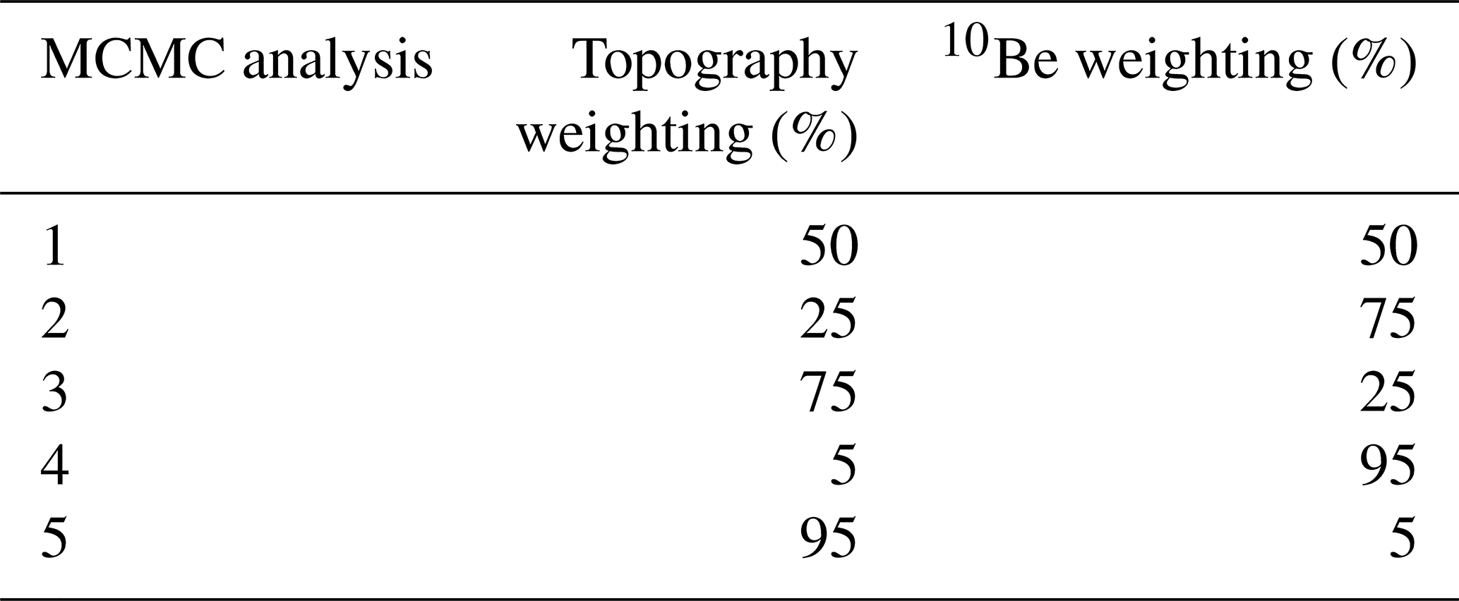
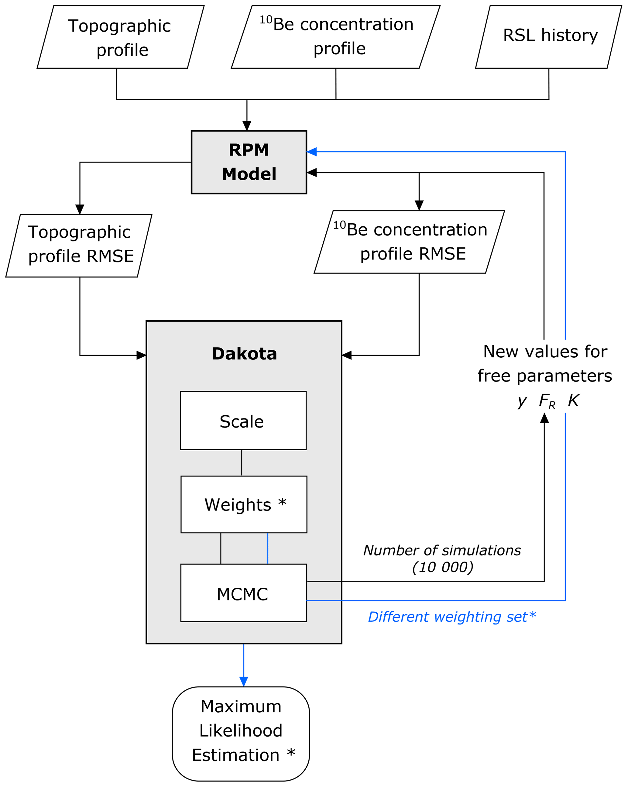
Figure 4Structure for implementing a single MCMC calculation using Dakota. Data inputs into the coupled model include a topographic profile, a 10Be concentration profile, and an RSL history. The MCMC analysis is performed multiple times with different weightings (shown by the blue loop) for the objective functions (topographic profile RMSE and 10Be concentration profile RMSE) and produces a corresponding maximum likelihood estimation (MLE*) result. For each MCMC calculation, the weights* value is changed for each RMSE score. The different values for the weights* are shown in Table 1 and correspond to wi (Eq. 2). The set of MLE results together produce the “Pareto front” of multi-objective optimised results.
3.3.4 MCMC analysis
Metropolis–Hastings is a specific MCMC implementation (Metropolis et al., 1953), in which MCMC is a class of methods based on Bayesian inference calibration. A detailed explanation of how Bayesian inference can be used to calibrate models is provided by Kennedy and O'Hagen (2001).
The composite likelihood score (Eq. 2) is calculated in Dakota; the lowest combined RMSE scores result in the maximum likelihood estimation (MLE). A so-called proposal distribution is used to select and jump to new parameter values within the MCMC algorithm. After each run, new values for the free parameters y, FR, and K (see Sect. 3.4) are randomly selected from a uniform proposal distribution centred at the current accepted parameter values. A likelihood ratio compares the posterior likelihood of the proposed parameter set to the previous accepted likelihood and is used to decide whether the new set of parameters is accepted or rejected. If the proposed parameter set produces a model result that is more likely than the current accepted parameter set (ratio of current to last accepted iteration>1), then the new parameter set is always accepted. If the proposed posterior is less likely (likelihood ratio<1), the new parameter set may still be accepted with a probability of acceptance proportional to the likelihood ratio (Hurst et al., 2016). This is achieved by generating a random number r from a uniform distribution between 0 and 1; if r<ratio, then the proposed parameter set is accepted. The Metropolis–Hastings algorithm allows for acceptance of less likely parameter sets in order to prevent the acceptance chain from reaching an immovable position in a localised likelihood trough. The proposal distribution variance was tailored so as to produce an acceptance rate of ∼23 % that ensures optimal chain mixing and full exploration of the parameter space (Gelman et al., 1997).
As we have no prior knowledge of the best-fit model parameters, a uniform prior distribution is used. As the prior distribution is essentially removed from the posterior probability calculation, Dakota returns best-fit parameter values that correspond to the MLE, which is similar to methods used to find optimal model results by Hurst et al. (2016). Dakota takes the log form of the likelihood function to help numerical stability by working with more manageable negative numbers and transforming from multiplications to additions. Minimising the negative log-likelihood is equivalent to maximising the likelihood.
3.3.5 Dakota functionality and constraining the parameter space
The parameter space is constrained to where modelled topographic profiles are similar to those observed at the selected study sites. The failure capture recovery option within Dakota is used to identify which combinations of input model free parameters cannot replicate the measured topographic profile sufficiently. A “fail” flag is produced by the model if the modelled shore platform profile does not erode to a width of at least the intertidal width of the measured shore platform profile. The width of the measured topographic profile (∼250 m) should be taken as the minimum width because the shore platform undoubtedly extends further offshore than where the UAV survey ended. A fail flag returned to Dakota is replaced by a high RMSE value (set to 999 999) so this combination of input model free parameters is avoided in future simulations within the Metropolis–Hastings algorithm.
3.4 MCMC analysis inputs
A previous investigation into the relative importance of wave erosion versus weathering using the RPM coastal evolution model found that wave erodibility, material resistance, and weathering rate parameters have the greatest influence on the dominance of erosional form (Matsumoto et al., 2018). Because these model variables have the greatest control over principal erosion processes, wave erodibility by means of wave height decay rate (y), material resistance (FR), and maximum intertidal weathering rate (K) are chosen to vary in the MCMC calculations (see Sect. 3.2.1).
Wave erodibility is explored in the MCMC analysis by varying the wave height decay rate (y), which is consistent with previous modelling approaches (e.g. Matsumoto et al., 2018; Trenhaile, 2000). Incident wave height is kept constant throughout model simulations. We chose to explore wave erodibility in the model by varying wave height decay rate (y) over incident wave height because a linear relationship between input wave height and material resistance (FR) is already established: greater wave height needs to be compensated for by an increase in material resistance (FR) (Matsumoto et al., 2016). Whereas by focussing on process dynamics with wave height decay rate (y) the spatial distribution and degree of wave erosion can be considered, varying the model parameter y will have implications for the shore platform morphology. Initial ranges of y followed Matsumoto et al. (2018) by varying an exponential value, a, between −2 and 1 (i.e. y=0.01–10 m−1), which, across a 200 m wide shore platform, would equate to wave height decreasing by 67 %–100 %. These wave attenuation rates are consistent with field-based observations of wave transformation across a shore platform. For example, Ogawa et al. (2011) find that wave height was reduced by ∼93 % across a 250 m wide platform at the lowest tidal stage. Wave height decay rate (y) is further constrained in this study to 0.01–0.16 m−1 because when values of y exceed 0.16 m−1 wave height would dissipate too quickly and wave force is not large enough to erode a shore platform to a distance that matches at least the width of the measured intertidal platform for both the Bideford and Scalby sites. These high values for y result in failed model runs as detected by the failure capture recovery function in Dakota (see Sect. 3.3.5).
For material resistance, we use a range of b (an exponential value) from 1–3 (i.e. FR=10–1000 kg m2 yr−1), which follows Matsumoto et al. (2018) and encompasses material resistance values used by other modelling studies that explore a range of rock strength settings; e.g. Trenhaile (2008a, b, 2000).
Following Matsumoto et al. (2018), maximum intertidal weathering rate (K) is varied as a proportion of the material resistance. The greatest rate of weathering that we apply is equal to FR×0.2 kg m2 yr−1, which results in maximum down-wearing rates of 20 mm yr−1 when only considering weathering contributions to shore platform down-wear. Down-wearing rates of 20 mm yr−1 are unrealistically high for a sandstone platform (e.g. Yuan et al., 2020). In this study, preliminary investigations were carried out to establish an appropriate range of weathering rates needed to match both objective functions at the two UK sites. Initial results for Bideford and Scalby showed that the topographic profiles and 10Be concentration profiles could only be well-matched simultaneously at very low to negligible weathering rates (K). Weathering of the shore platform surface becomes negligible when weathering rates (K) fall below a particular ratio in relation to material resistance (FR). By calculating the weathering rate (K) (kg m2 yr−1) for the full modelled simulation time (K×8000 years), we can compare the total value for K to the value of FR to detect when weathering rate (K) is less than the material resistance (FR). We find that when the exponent of , maximum weathering rate falls below the value for material resistance (FR) for the simulated model time, and erosion of the shore platform through weathering processes becomes negligible because rock cells cannot be removed from the model array by means of subaerial weathering. The range of c was adjusted to −10 to −4 for Bideford and −10 to −1 at Scalby to ensure negligible weathering was included within the MCMC analysis parameter space. At Scalby, 10Be concentrations can still be matched at higher rates of weathering; therefore, we include the upper range of K values in the MCMC analysis. The wide range of weathering rates that we explore are similar to equivalent platform down-wear rates quantified for a range of field-based studies (e.g. Buchanan et al., 2020; Moses, 2014; Stephenson et al., 2019; Swirad et al., 2019).
In order to replicate a full range of platform geometries, we vary these parameters over several orders of magnitude across a range that was guided by previous exploratory morphodynamic modelling (Matsumoto et al., 2016, 2018). We need to not only apply effective proposal distributions to the free parameters that ensure the full parameter space is explored, but also achieve optimal acceptance rates (see Sect. 3.3.4). In order to target optimal acceptance rates and fully explore the parameter space, exponents of the y, FR, and K variables are treated as the calibration parameters, which is similar to approaches taken by Barnhart et al. (2019), and these values are varied between model runs. Symbology assigned to the exponent calibration parameters are a for y, b for FR, and c for K, which are summarised in Table 2.
As these parameters are abstractly defined within the model, it is important to highlight that our aim is not to report accurate wave force, weathering rates, and material strength at real-world sites but to determine the best combination of model parameters to match measured datasets in order to model cliff retreat. Table 2 summarises the ranges of the free parameters y, FR, and K used in the MCMC analysis.
Table 2Free variables, corresponding calibration parameters and their units, and lower and upper bounds used in the MCMC calculations.

3.5 Interpretation of results
The best-fit parameter results provided by Dakota, which correspond to the set of parameters with the MLE, are used for the model results that best fit the measured data. Likelihood-weighted histograms are constructed from the distribution of accepted MCMC samples for each of the free parameters. Confidence intervals defined by the 16 % and 84 % percentiles of the distributions are used as the uncertainty for the best-fit parameter values. We choose not to use 5 % and 95 % confidence intervals because the resultant range of model outputs produces unrealistic uncertainty for the modelled topographic profile in terms of the range in platform elevations and gradients. To observe the resultant uncertainty of model outputs as defined by the MCMC results, ensemble runs of the coupled model explore the median as well as the 16 % and 84 % confidence range for each parameter against the median result of the other two parameters. A total of nine model outputs for each site are produced.
4.1 Pareto set of optimised results
A Pareto set was constructed by performing multiple MCMC inversions with different weightings given to the two objective functions (see Sect. 3.3.3). Because we use measurement error to scale each objective function, there is potential for bias as a result of the relative precision of both measured datasets. It was necessary to explore a range of weightings for the objective functions to understand the impact of measurement error on the model outputs and to explore how sensitive the final best-fit model outputs were to changes in the dominant objective function.
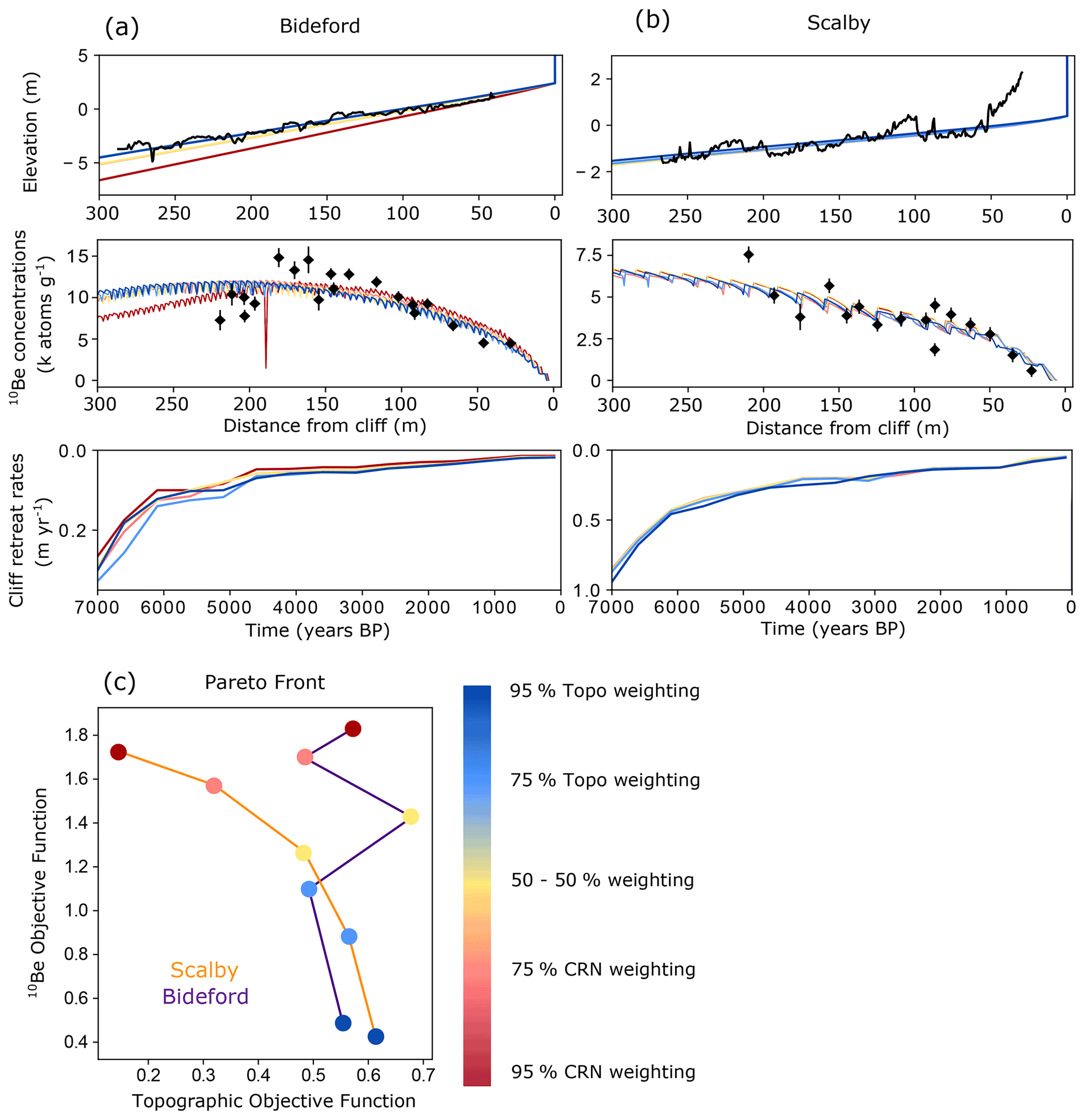
Figure 5The five Pareto set results for both the Bideford (a) and Scalby (b) sites. The modelled topographic profile and 10Be concentration profile are shown alongside corresponding measured data. Modelled cliff retreat rates are shown for the past 7000 years. The yellow model results correspond to 50 %–50 % objective-function-weighted MCMC results. The darkest blue model results correspond to the MCMC results that were most weighted towards the topographic (Topo) profile (95 %). The darkest red model results correspond to the MCMC results that were most weighted towards the 10Be concentration (CRN) profile (95 %). The Pareto front of scaled and weighted 10Be and topographic objective functions is shown for both sites (c).
The Pareto set of MCMC best-fit results for the Bideford site is shown in Fig. 5a. All combinations of objective function weightings, except for the MCMC analysis weighted most towards the 10Be concentration profile (shown in darkest red), fit both measured datasets well. The saw-tooth pattern seen in the 10Be concentration profile is caused by the cell framework resolution of the model. When a surficial rock cell with greatest 10Be concentrations is eroded and removed from the rock profile, 10Be concentrations drop as a subsurface cell with less 10Be is revealed. The MCMC best-fit result with 95 % weighting assigned to the 10Be concentration profile and 5 % assigned to the topographic profile results in a topographic profile that is considerably steeper than the measured profile at Bideford. We do not want to base modelled cliff retreat rates on scenarios that are not able to replicate the topography of the shore platform profile well and so should avoid weighting too strongly towards the 10Be concentration profile. For the Pareto front, where the scaled and weighted topographic and 10Be concentration objective functions are compared, the sensitivity of different weighting sets to final model results at Bideford is revealed (Fig. 5c). The Pareto set at Bideford again suggests we should weight more towards the topography, but only when we weight the combined objective function 95 % towards the 10Be concentration profile RMSE do we see a poor match to the topography (Fig. 5a).
Dissimilarly, at Scalby, all combinations of objective function weightings produce very similar model outputs (Fig. 5b). This reveals that the best-fit model results for the topographic profile and the 10Be concentration profile are found in the same parameter space for Scalby but not necessarily for Bideford. Uniformity in results across the Pareto set for Scalby is further supported by the Pareto front (Fig. 5c). For Scalby, the Pareto front shows the expected convex shape of a Pareto front that looks to minimise both objective functions simultaneously.
Crucially, final results from the 50 %–50 % weighted MCMC analysis show a good representation of the full Pareto set of output model results (Fig. 5). We suggest that future applications can confidently use a single, equally weighted multi-objective MCMC calculation to optimise the coupled model to multiple measured datasets and quantify modelled cliff retreat rates. Subsequently, results from the equally weighted MCMC analysis are used to construct final model outputs and objective function surfaces in following sections. Results from all weighted MCMC calculations can be found in Table S8 in the Supplement.
4.2 Best-fit model results
Model outputs using the best-fit results and uncertainty defined by the 50 %–50 % weighted MCMC results show that the coupled model is able to produce a good fit to both the topographic profile and 10Be concentration profile for both sites (Fig. 6). The topographic profiles shown are the present-day positions (time 0 kyr BP). For the topographic profile, maximum uncertainty in the elevation range is found furthest offshore from the cliff. For the intertidal platform width, where measured data were collected, maximum uncertainty in elevation is ∼5 m (300 m offshore from the cliff) at Bideford (Fig. 6b) and ∼1 m (300 m offshore from the cliff) at Scalby (Fig. 6f). The nearshore increase in the measured platform slope seen at Scalby is the start of the beach profile. Modelled 10Be concentrations display the characteristic humped profile (Regard et al., 2012) (Fig. 6c and g) with maximum variance in 10Be concentrations occurring offshore of the “hump” at both sites. Maximum uncertainty in modelled 10Be concentrations for the intertidal platform is ∼5000 atoms g−1 at Bideford (Fig. 6d) and ∼2500 atoms g−1 at Scalby (Fig. 6h). These uncertainties are proportional to the magnitude of the measured concentrations with peak 10Be concentration of 14 818 atoms g−1 at Bideford and 7547 atoms g−1 at Scalby.
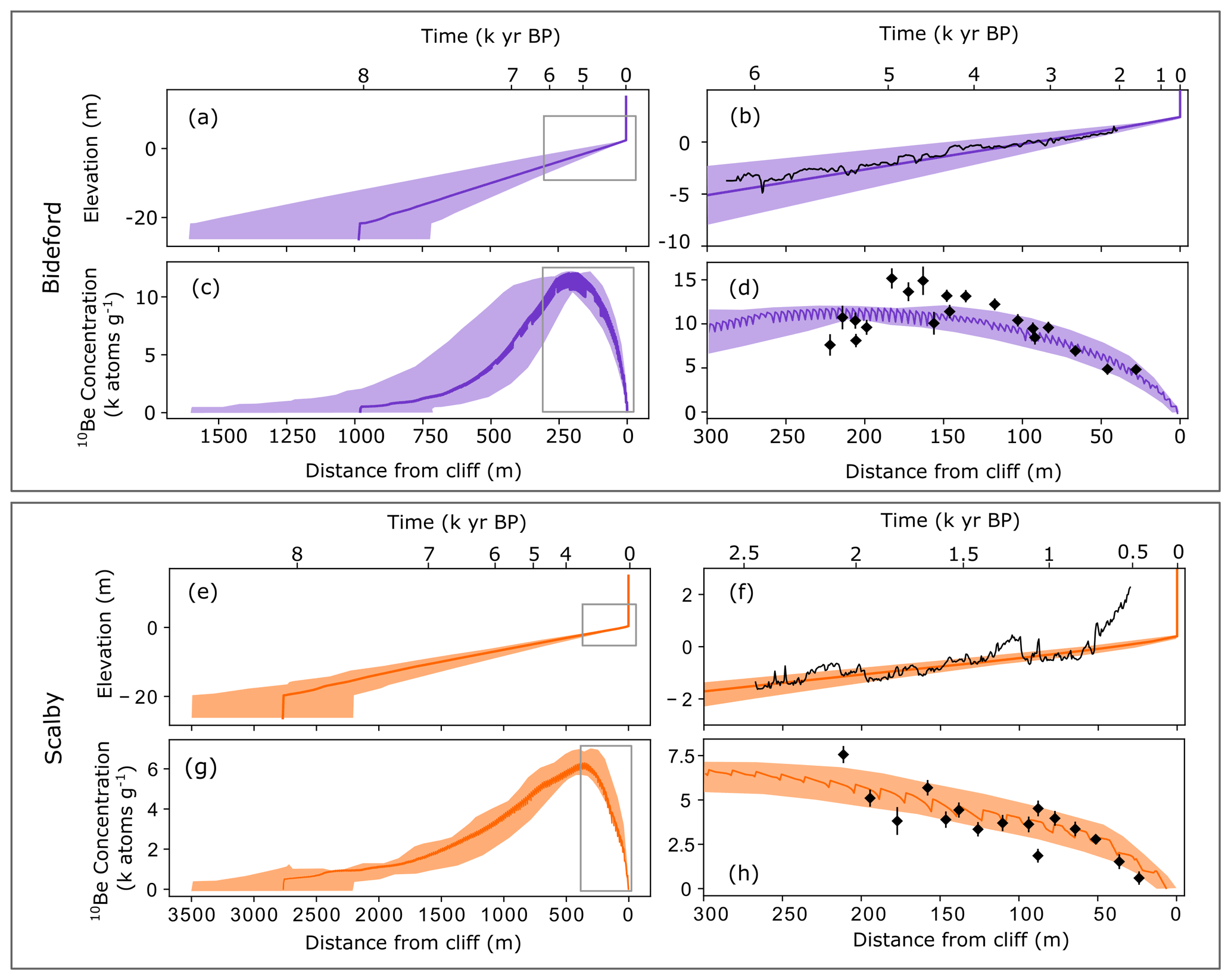
Figure 6Final results from the 50 %–50 % weighted multi-objective MCMC calculation for the Bideford study site (a, b, c, d; shown in purple) and Scalby study site (e, f, g, h; shown in orange). Dark lines show the best-fit results, and the shaded areas show the confidence interval uncertainty range. The 16 %–84 % confidence interval for each parameter (FR, K, and y) was simulated against the median results for the other parameters, and shaded uncertainty regions were constructed from the upper and lower limits of model outputs. Panels (a) for Bideford and (e) for Scalby show the full width of the modelled topographic profile. Panels (b) for Bideford and (f) for Scalby show the first 300 m of the modelled platform offshore from the cliff (0 m) and compare modelled results to the measured topographic profile (black solid line). Panels (c) for Bideford and (g) for Scalby show the full modelled extent of the 10Be concentration profile. Panels (d) for Bideford and (h) for Scalby show the first 300 m of the modelled 10Be concentration profile offshore from the cliff (0 m) and compare modelled results to the measured and corrected 10Be concentrations (see Sect. 3.1). Grey boxes (a, c, e, g) correspond to 300 m distance offshore (b, d, f, h). Time stamps for the cliff positions across the 8000-year-duration simulation time were back-calculated and shown against corresponding cliff positions.
At Bideford, the best-fit modelled scenarios show that the platform has eroded to a width of 750–1650 m across the past 8000 years (Fig. 6a). At Scalby, however, the best-fit modelled scenarios indicate that the platform has eroded to a wider width of 2200–3500 m (Fig. 6e) over the same time period. Time stamps for modelled cliff positions are back-calculated and shown for the corresponding distance across the shore platform. For example, the modelled cliff position at Bideford was 200 m offshore from the present-day cliff position at ∼5000 years BP (Fig. 6b). These time stamps correspond to when the horizontal position of the cliff foot was there, but not the exact elevation because down-wearing has occurred since. Our results indicate that the 250 m present-day intertidal platforms at Bideford and Scalby were eroded in the past 5800 and 2400 years, respectively (Fig. 6). The less time taken to erode the same distance of shore platform at Scalby indicates that late Holocene cliff retreat rates at Scalby are over 2 times faster than at Bideford. As the magnitude of the measured 10Be concentrations at Scalby is considerably less than at Bideford, this model result aligns with model predictions of CRN concentrations and cliff retreat rate interpretations, i.e. that the magnitude of CRN concentrations is inversely proportional to cliff retreat rates.
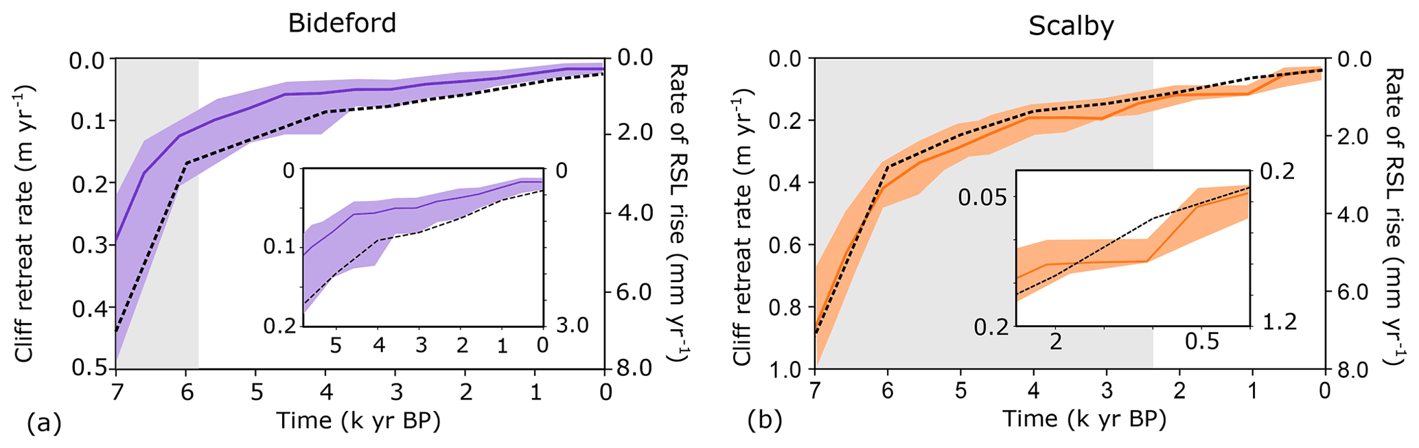
Figure 7A time series of cliff retreat rate (m yr−1) shown by the solid line and shaded area across the late Holocene (from 7000 years BP to the present day) calculated from modelled cliff positions every 100 years. The first 1 kyr is excluded as this corresponds to the burn-in period of the model. The rate of RSL rise (mm yr−1) is shown alongside cliff retreat rates by the dashed black line. Inset plots show the cliff retreat rates and rate of RSL rise for the time period that corresponds to the distance across the shore platform over which measured data were analysed (∼250 m). For Bideford (a), the past 5800 years of modelled cliff retreat correspond to the 250 m intertidal shore platform. For Scalby (b), the past 2700 years of modelled cliff retreat correspond to the 250 m intertidal shore platform. The grey shaded area corresponds to the cliff retreat rates which occurred further offshore than where the measured data were collected, and the non-shaded area shows the extent of the inset plots.
A time series of cliff retreat rates, which are calculated from modelled cliff positions every 100 years, shows a decline in cliff retreat rates across the Holocene (Fig. 7). The evolution of modelled cliff retreat covered by the across-shore distance of measured data encompasses the past 5800 years at Bideford (Fig. 6b) and the past 2400 years at Scalby (Fig. 6f). We are only able to report cliff retreat rates with confidence for these time periods which correspond to the measured datasets. Following this, the model results for Bideford show that cliff retreat rates have declined from 7.5–17.5 cm yr−1 at 5800 years BP to 1–3 cm yr−1 at the present day (Fig. 7a). Likewise, the model results for Scalby show that cliff retreat rates have declined from 11–17 cm yr−1 at 2400 years BP to 4–8 cm yr−1 at the present day (Fig. 7b). Despite lacking measured data beyond 250 m offshore from the cliff, we can assess the antecedent modelled cliff retreat rates needed to match the modelled to measured profiles in the intertidal zone (full extent of grey areas in Fig. 7). Best-fit model results for the full model simulation time reveal a declining cliff retreat rate scenario for both sites. At Bideford, cliff retreat rates decline from 25–55 cm yr−1 at 7000 years BP to 1–3 cm yr−1 at the present day (Fig. 7a). Similarly, at Scalby, cliff retreat rates decline from 70–100 cm yr−1 at 7000 years BP to 4–9 cm yr−1 at the present day (Fig. 7b).
The best-fit scenario of a declining cliff retreat rate throughout the Holocene directly reflects the pattern of decline in the rate of RSL rise for both UK sites. At Bideford, the rate of RSL rise falls from +2.5 mm yr−1 at 5800 years BP to +0.5 mm yr−1 at the present day (Fig. 7a). Similarly, at Scalby the rate of RSL rise falls from +1.1 mm yr−1 at 2700 years BP to +0.3 mm yr−1 at the present day (Fig. 7b).
Table 3Best-fit parameter results from 50 %–50 % weighted, multi-objective MCMC calculations.
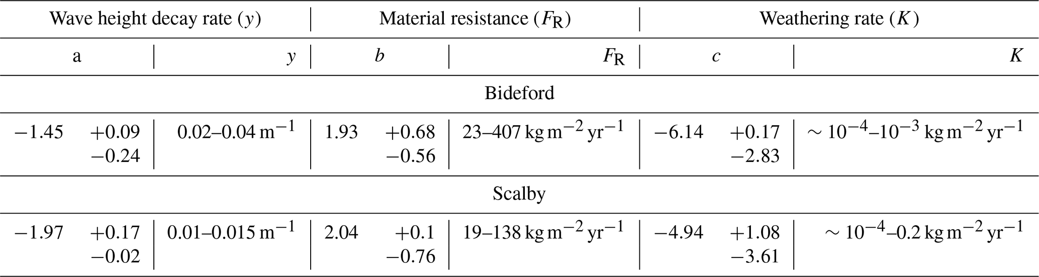
Table 3 summarises the results from the 10 000-iteration, equally weighted MCMC analysis for both sites, with uncertainties defined by the 16 % and 84 % confidence intervals of the likelihood-weighted accepted sample distributions. Acceptance rates for all MCMC calculations ranged between 17 % and 40 % and therefore encompass the range of optimum acceptance rates for chain mixing (Gelman et al., 1997). Figures S1 and S2 in the Supplement plot the cumulative moving median as well as the 16 % and 84 % quantiles across the 10 000 iterations to show the MCMC burn-in period. We found that 10 000 iterations for each weighted MCMC analysis was a sufficient number of samples to build robust posterior distributions.
4.2.1 Material resistance (FR)
Posterior MCMC results of accepted samples show that the topography and 10Be concentration profiles can be well-matched across a large range of FR values (Table 3). For Bideford, the best-fit result defined by the 16 %–84 % confidence intervals for the equally weighted multi-objective MCMC analysis for FR is equivalent to 23–407 . For Scalby, best-fit results for FR tend towards lower values for material resistance of 19–138 . The large uncertainty for FR from posterior distributions is caused by correlation found between FR and y (see Sect. 5.2).
4.2.2 Weathering rates (K)
At both sites, low to negligible weathering rates (K) as a proportion of material resistance (FR) are needed to match both measured datasets simultaneously. At Bideford, the best-fit results for maximum weathering rate are skewed towards the lowest K values. Both measured datasets could only be well-matched when negligible weathering was implemented in the modelled profile evolution. Best-fit results for K range across orders of magnitudes (–10−3 ) when applying the best-fit result for FR (85 ). Using the upper limit of FR and K defined by 84 % confidence intervals, the absolute maximum weathering rate acting on the profile at Bideford is equivalent to 0.03 . This weathering rate would result in maximum down-wear rates equivalent to 0.007 mm yr−1 when only considering down-wear as a result of intertidal platform weathering. These results indicate that erosion of the shore platform at Bideford is dominated by wave-driven erosion.
In comparison to Bideford, at Scalby, maximum weathering rates acting on the shore platform surface (K) best match the measured data at intermediate to low weathering rates equivalent to ∼0.0001–0.27 when using the best-fit result of FR (109 ). This weathering rate would result in maximum down-wear rates equivalent to 0.2 mm yr−1 if only considering down-wear as a result of intertidal platform weathering. Although weathering rates are still low at Scalby, distinctions between the two sites in relation to maximum weathering rates can still be made. Observing objective function surfaces (see Sect. 4.3) can help explain the differences between the two UK sites in terms of weathering-controlled erosion of the shore platform and the match to both the measured topography and 10Be concentrations. This, in turn, can reveal if and where any compromises had to be made to match both objective functions, e.g. if the two individual objective functions are not minimised in the same area of the parameter space.
4.2.3 Wave height decay rates (y)
Results from the wave height decay rate (y) show that Scalby best-fit results tend towards the lowest wave height decay rates, which are equivalent to 0.01–0.015m−1. Or, in other words, breaking waves exert erosive power across the furthest distance possible based on realistic constraints placed on y (see Sect. 3.4). Bideford, on the other hand, has best-fit y values at higher wave height decay rates, with a best-fit value equivalent to 0.02–0.04 m−1. The larger value for y means wave height will dissipate faster and cover a shorter distance across the shore platform at Bideford in comparison to Scalby.
4.3 Objective function results
Observing the objective function space for the topographic RMSE, 10Be concentration RMSE, and the combined likelihood helps demonstrate the trade-offs between the three different parameters (FR, K, and y) and the effects on the two objective functions. In the following sections, when addressing the unitless values for the free parameters, we are referring to the exponential calibration parameters (a, b, c) that were varied in the MCMC calculations (see Sect. 3.4).
4.3.1 Material resistance vs. weathering rate
Comparisons between calibration parameters varied for material resistance (b) and weathering rate (c) show no distinctive influence on the endmember topographic profile at the Bideford site (Fig. 8a). In contrast, only once c falls below −5 and weathering rates become negligible can the modelled 10Be concentration profile closely replicate the measured data (Fig. 8b). Furthermore, with insignificant active weathering, combinations between material resistance and weathering rate show no noteworthy influence on the modelled 10Be concentration profile. The likelihood objective function for the accepted samples shows that the best samples are generally found when c is below −5 (Fig. 8c). Results from initial Bideford MCMC calculations, with the range of c set to −5 to −1, are found in the Supplement and show that the 10Be concentrations cannot be matched with the higher range of weathering rates explored initially (Fig. S3 in the Supplement). There needs to be negligible intertidal weathering of the shore platform in order to produce the relatively high 10Be concentrations measured at the Bideford site. This is only revealed when optimising for the 10Be profile; optimising for the topographic profile alone, however, does not reveal any distinct behavioural trends between b and c.
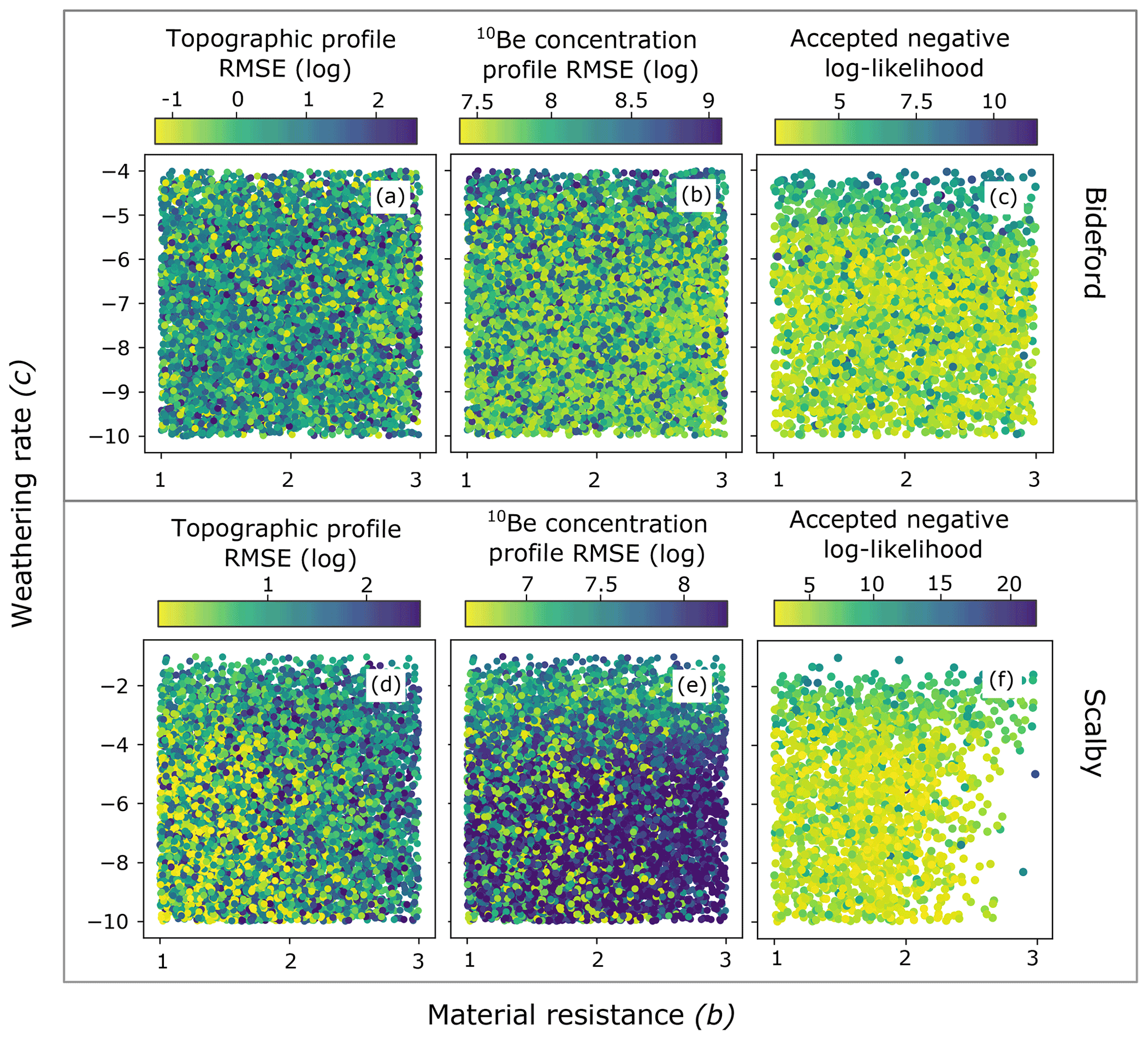
Figure 8Objective function results for the material resistance (b) and weathering rate (c) parameters constructed from 50 %–50 % weighted MCMC analysis results for the Bideford site and Scalby site. The topographic profile RMSE (a, d) and 10Be concentration profile RMSE (b, e) objective function spaces are constructed from all 10 000 samples visited in the MCMC analysis. The combined likelihood objective function space (c, f) is constructed just using the accepted samples from the MCMC analysis. Dark blue corresponds to the worst samples that have the highest RMSE and negative log-likelihood scores, while bright yellow corresponds to the best samples that have the lowest RMSE and negative log-likelihood scores.
At Scalby, comparisons between b and c show that a better fit to the topographic profile can generally be found at the lower range of b and c (Fig. 8d). In contrast, the 10Be concentration profile can be well-matched at higher weathering rates with c of −2 (Fig. 8e). These results contrast with the results from Bideford, which show that negligible weathering needs to occur in order to match the 10Be concentration profile. However, these relationships are not well-defined: well-matched 10Be concentration profiles can still be produced when weathering rates are low (Fig. 8e). Equally poorly matched topographic profiles can still be produced at the lower range of b and c (Fig. 8d). This suggests that the third free parameter varied in the MCMC analysis, wave height decay rate (a), has a further influence on the final modelled profiles. For both sites, these results strongly imply that wave-driven erosion dominates over subaerial weathering in the long term.
4.3.2 Wave height decay rate vs. weathering rate
For Bideford, a clear zone in the mid-range of wave height decay rates () produces well-matched topographic profiles across the full range of weathering rates (c) (Fig. 9a). When , a threshold exists where a zone of well-matched topographic profiles suddenly meets a zone of poorly matched topographic profiles. When wave height decay rate (a) is increased too much, waves will dissipate their energy too quickly and will result in modelled topographic profiles with gradients too steep to match the topographic profile at Bideford.
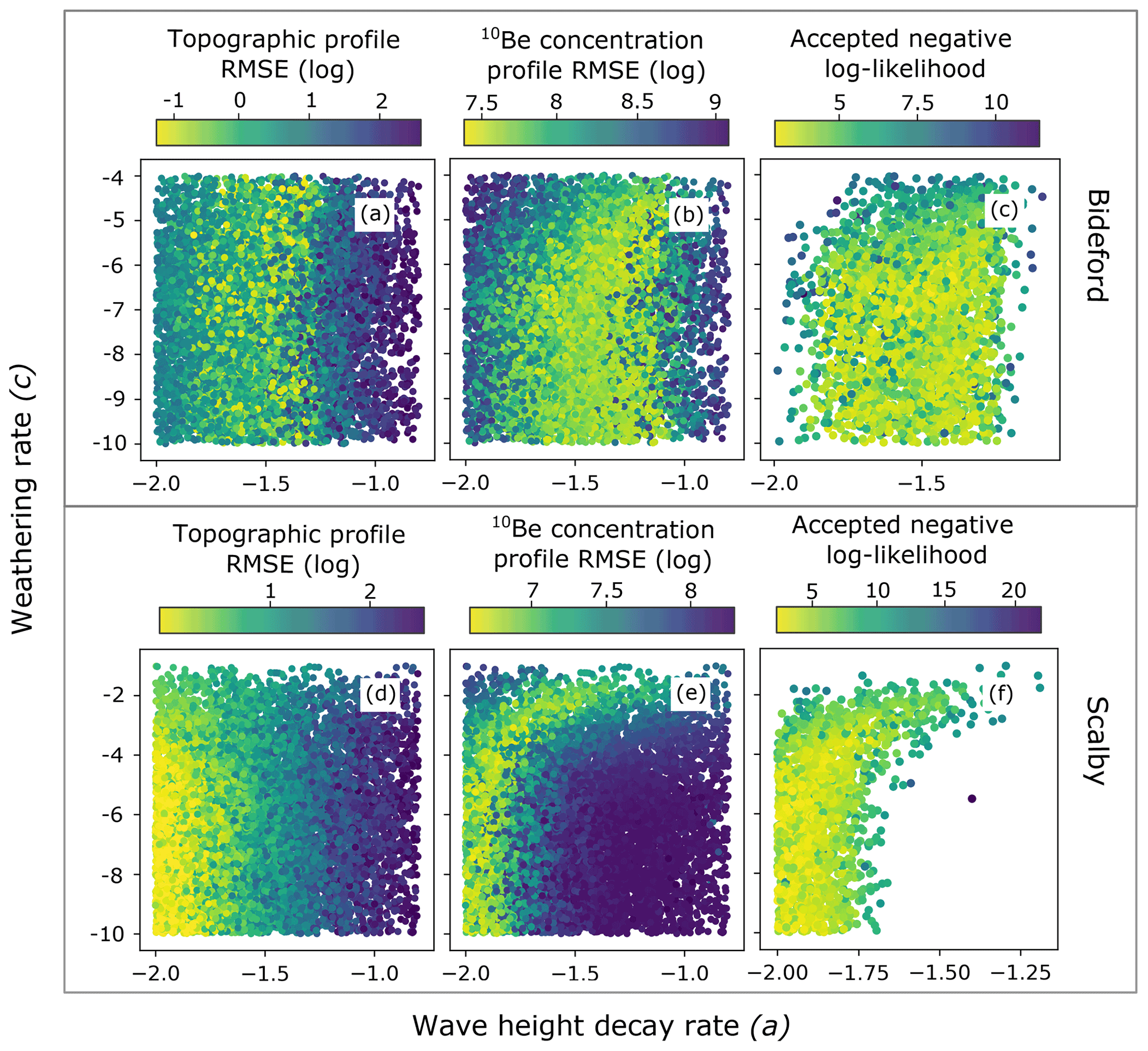
Figure 9Objective function results for the wave height decay rate (y) and weathering rate (K) parameters constructed from 50%–50 % weighted MCMC analysis results for the Bideford and Scalby sites. The topographic profile RMSE (a, d) and 10Be concentration profile RMSE (b, e) objective function spaces are constructed from all 10 000 samples visited in the MCMC analysis for Bideford and Scalby, respectively. The combined likelihood objective function space (c, f) is constructed just using the accepted samples from the MCMC analysis. Dark blue corresponds to the worst samples that have the highest RMSE and negative log-likelihood scores, while bright yellow corresponds to the best samples that have the lowest RMSE and negative log-likelihood scores.
When considering the influence on the 10Be concentration profile at Bideford, a much wider zone across the range of a produces well-matched 10Be concentration profiles when , i.e. when there is negligible subaerial weathering occurring (Fig. 9b). This zone of well-matched 10Be concentration profiles extends across the boundary where good and bad topographic profiles can be produced (Fig. 9a). The addition of 10Be concentrations to the objective function results in a dense zone of accepted samples across a range for a of to −1.3 when (Fig. 9c).
In contrast to Bideford, the slowest wave height dissipation across the shore platform (defined by the lowest a values) produces the best topographic profile seen at Scalby (Fig. 9d). Only when assessing the 10Be concentration profile are we able to see how weathering rates interact with wave erosion to impact the model results for Scalby (Fig. 9e). Slower wave height dissipation requires lower rates of weathering in order to produce a matching 10Be concentration profile. In the zone of well-matched results, as wave height decay rate (a) values decrease, weathering rates also decrease (Fig. 9e). Because the peak in 10Be concentrations at Scalby is ∼7000 atoms g−1 less than the peak in 10Be concentrations at Bideford, greater weathering rates and, as a result, greater platform lowering can produce a modelled 10Be profile that matches the measured data for Scalby. As active subaerial weathering can contribute to model outputs that can replicate the measured data, the balance of wave-driven and weathering-controlled erosion is more complex at Scalby. Wave erosion and weathering can trade off in multiple combinations to produce model outputs that match both the measured 10Be concentration profiles and topographic profiles at Scalby. The accepted samples (Fig. 9f) show that the best model results are found at the lower range of y when constrained by matching to the topographic profile (Fig. 9d) and 10Be profile (Fig. 9e) simultaneously.
4.3.3 Wave height decay rate vs. material resistance
A distinct negative relationship exists between material resistance (b) and wave height decay weight (a) at Bideford when optimising to the topographic profile (Fig. 10a). As b increases, more wave energy is needed to erode the cliff at a rate fast enough to produce a shore platform with a gradient shallow enough to match that seen at Bideford. In other words, wave height decay rate has to be reduced so waves can dissipate their energy across a further distance. Varying the wave decay rate (a) for any value of b reveals a distinct zone where wave energy is high enough to produce a wide enough platform, but not large enough to decrease the profile slope to below the observed 0.02 gradient at Bideford. The same relationship exists when optimising for the 10Be concentration profile, but the best region has shifted to a zone with a greater wave height decay rate (Fig. 10b). This ratio between a and b strongly controls the accepted results for Bideford (Fig. 10c). Section 5.2 expands on this correlation found between the a and b parameters.
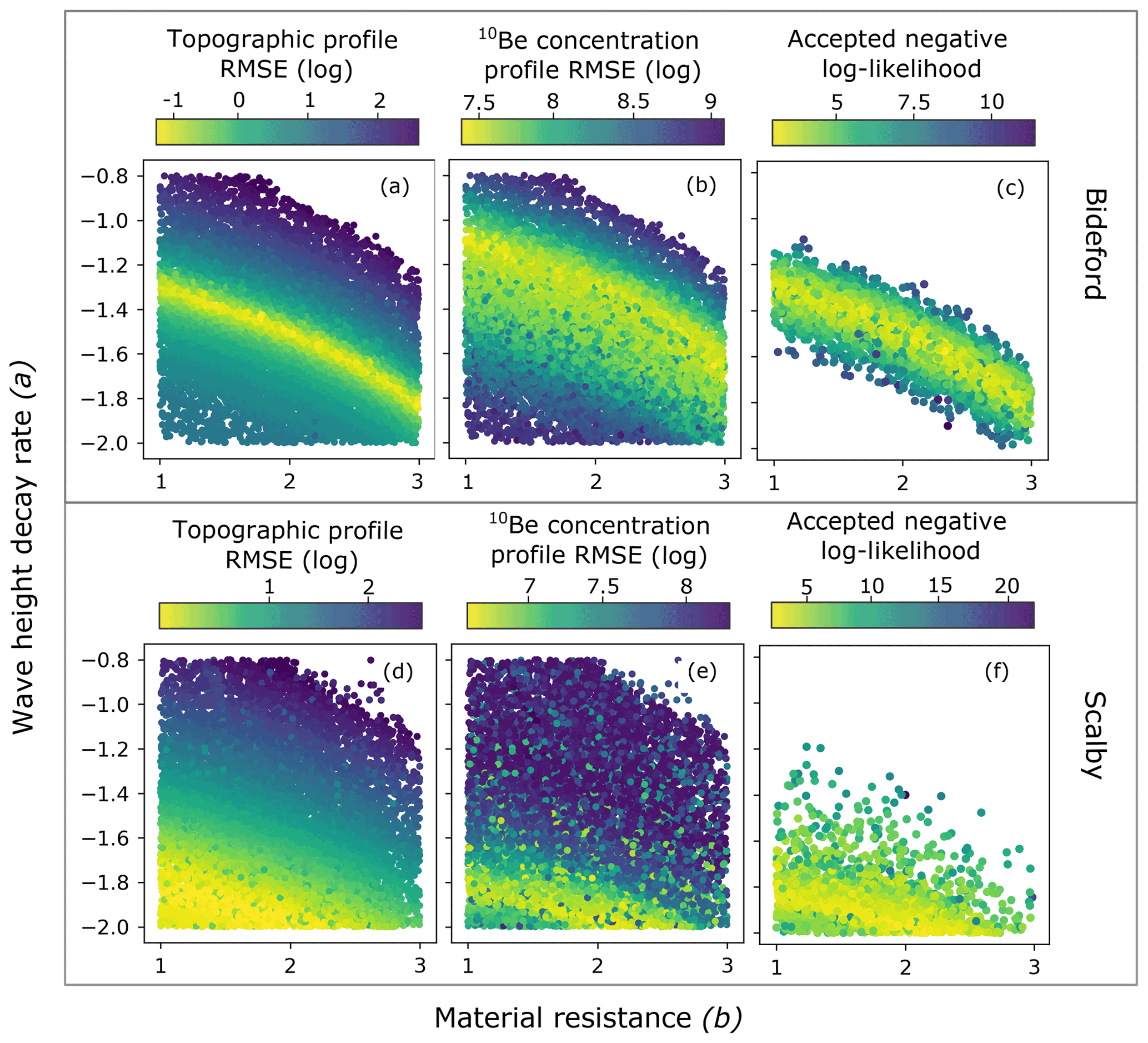
Figure 10Objective function results for the material resistance (b) wave height decay rate (a) parameters constructed from 50 %–50 % weighted MCMC analysis results for the Bideford site and Scalby site. The topographic profile RMSE (a, d) and 10Be concentration profile RMSE (b, e) objective function spaces are constructed from all 10 000 samples visited in the MCMC analysis. The combined likelihood objective function space (c, f) is constructed just using the accepted samples from the MCMC analysis. Dark blue corresponds to the worst samples that have the highest RMSE and negative log-likelihood scores, while bright yellow corresponds to the best samples that have the lowest RMSE and negative log-likelihood scores.
For Scalby, there is a similar, but less distinctive, trade-off between a and b as seen at the Bideford site. A wider range of wave height decay rates (a) is able to produce a suitable topographic profile in relation to b with the most likely results tending towards lower rates of wave height decay rate (a) (Fig. 10d). The platform gradient is shallower at Scalby (0.01); once a falls below , a shallow platform gradient can be produced by a wider range of wave height decay rate values as long as material resistance (b) is relatively low. The influence of the 10Be concentration optimisation constrains the window of best results (Fig. 10e). Accepted samples cover a wider area of the parameter space at Scalby compared to Bideford (Fig. 10f).
Our ultimate aim is to quantify the long-term history of transient cliff retreat rates in order to enable better predictions of future cliff retreat rates at rock coast sites across the UK and worldwide. Our results show that rigorous multi-objective optimisation of a process-based coastal evolution model to high-precision measured datasets permits long-term trajectories of cliff retreat to be identified and quantified for real-world sites over centennial to millennial timescales.
To explore the potential for further application of these methods at other rock coast sites, here we justify the methodology chosen, address equifinality in model results, and explore how equifinality impacts our ability to quantify cliff retreat rates. We also highlight some aspects of our results that should be interpreted with caution, specifically where correlation exists between parameters.
5.1 The importance of multi-objective optimisation
In this study, we have a rare opportunity to formally evaluate how two distinctive datasets constrain a model differently. We find that the two datasets used here reveal dissimilar patterns in the objective function space between the topographic profile RMSE and the 10Be concentration RMSE (Figs. 8–10). The topographic data and 10Be concentration data have therefore provided us with different information and validate the use of multi-objective optimisation in understanding the long-term evolution of rock coasts.

Figure 11Objective function surface at Bideford (a) for the parameters material resistance (b), material weathering rate (c), material resistance (b), and wave height decay rate (a). The blue shaded region (a) shows where in the parameter space the modelled topographic profile alone can match measured data. Blue diamonds (a) correspond to example model results shown in (b). The orange shaded region (a) shows where in the parameter space the modelled 10Be concentration profile alone can match measured data. Orange triangles (a) correspond to example model results shown in (c). The pink shaded region (a) shows where in the parameter space both the modelled topographic profile and 10Be concentration profile can match measured data. Pink crosses (a) correspond to example model results shown in (d). Cliff retreat rates (m yr−1) on a log scale for each set of model examples are shown in (e). Model results are from the 50 %–50 % weighted Pareto set simulation.
Using the results from Bideford as an example, we can observe model outputs for three different zones within the parameter space: (1) zones where we are able to match the topographic profile, but not the 10Be concentration profile; (2) zones where we are able to match the 10Be concentration profile, but not the topographic profile; and (3) zones where we are able to match both objective functions. At the Bideford site, the parameter space that can produce model results that match the topographic profile well but the 10Be concentration profile poorly is only found where weathering rates are high () (shaded blue, Fig. 11a). Examples of model outputs from this area (Fig. 11a) of the parameter space show that the shore platform gradient and elevation can be matched well, but the magnitude of all modelled 10Be concentration profiles is considerably lower than the corresponding measured data (Fig. 11b). This upper range of weathering rates (c) was incorporated into the initial MCMC analysis for the Bideford site, but was adjusted in later simulations because the model could not produce well-matched 10Be concentration profiles for this range of c (see Sect. 3.4). If we only optimise to the modelled topographic profile, we could vastly overestimate the contributions of weathering to the shore profile evolution at Bideford. More importantly, modelled cliff retreat rates are consistently faster than the multi-objective optimised retreat rate results that also try to match 10Be concentrations (Fig. 11e).
Furthermore, the zone where model outputs can match the 10Be concentration profile, but cannot match the topographic profile, is shown for the parameter space between material resistance (b) and wave height decay rate (a) (shaded orange, Fig. 11a). In all corresponding model examples shown (Fig. 11c), the magnitude of the 10Be concentration profile matches the measured data well, but modelled shore platform profiles are steeper than the measured topographic profile. As wave height decay rate values (a) are increased above the parameter space that is able to match both objective functions well (shaded pink, Fig. 11a), the reduction in wave erodibility produces steeper profiles because erosion is less efficient. Concentrations of 10Be are highly dependent on the evolution of the surface topography. Therefore, even if we are able to match 10Be concentrations to corresponding data, if the topography is incorrect, we are matching the 10Be concentrations incidentally and not as a result of correct topographic evolution. Results that can only match 10Be concentrations should therefore be discarded.
Finally, the parameter space where both the topographic profile and 10Be concentration profile can be matched well is shown (shaded pink, Fig. 11a). This zone corresponds directly to the most likely accepted samples (Fig. 10). Examples of model outputs across this zone all show a good fit to the topographic profile and 10Be concentration profile (Fig. 11d). The reduced area covered by the pink shaded region demonstrates how optimising to multiple datasets has considerably reduced uncertainty in final best-fit parameter results.
Results from topographic-only optimisation (shaded blue, Fig. 11e) show the same declining trend in cliff retreat rates, but are overall consistently faster than the rates of cliff retreat generated from multi-objective optimisation (shaded pink, Fig. 11e). Furthermore, uncertainty in topographic-only optimised retreat rates is much greater compared to multi-objective optimisation results, particularly in modern-day modelled cliff retreat rates. In contrast, results from 10Be-concentration-only optimisation (shaded orange, Fig. 11e) produce slower cliff retreat rates when compared to the multi-objective optimised results but still show the declining trend. Multi-objective optimised results (shaded pink, Fig. 11e) show the declining trend in cliff retreat rates with magnitudes intermediate to the two single-objective function results. Importantly, the range of retreat rates from multi-objective optimisation is considerably smaller in comparison to single-objective optimisation. Present-day cliff retreat rates based on multi-objective optimisation range from 1.8–2 cm yr−1 in contrast to 10Be-concentration-only cliff retreat rates of 1–1.5 cm yr−1 and topographic-only optimisation cliff retreat rates of 3–9 cm yr−1.
Differences between cliff retreat rates on the scale of centimetres per year (cm yr−1) may not appear noteworthy, but projecting these retreat rates across large temporal scales has a significant effect on the modelled rock coast erosional history. For example, the 250 m modern-day intertidal shore platform would have been eroded in the past 2700–5200 years based on topographic-only optimisation, 6800–7000 years based on 10Be-concentration-only optimisation, and 5400–5600 years based on multi-objective optimisation. For these examples, the time period of modelled cliff erosion that reflects a good match to the measured topographic profile results in an uncertainty of 2500 years, whereas an uncertainty based on multi-objective optimisation is only 200 years. The example rock coast site at Bideford is a stable coastline with relatively slow historic cliff retreat rates. It is important to ensure that modelled cliff retreat rates can be constrained as much as possible because the magnitude and uncertainty in cliff retreat rates would increase by orders of magnitude when applying this model to more dynamic rock coast sites, such as the southern UK coast chalk cliffs that are currently retreating at a much faster rate (e.g. Hurst et al., 2016).
Multi-objective optimisation ensures that we optimise both objective functions simultaneously and that best-fit results will reflect the parameter space where both measured datasets can be well matched. Consequently, equifinality in best-fit results can be substantially limited, which, most importantly, results in better-constrained modelled cliff retreat rates. Further improvements to the model optimisation may be made with future inversion calculations by optimising to a third measured dataset, including a second CRN concentration profile (e.g. 26Al or 14C). This has the potential to (1) further constrain modelled long-term cliff retreat rates and (2) reveal more complex shore platform erosion evolution through coupled CRN analysis such as platform burial due to sediment cover.
5.2 Parameter correlation
As previously mentioned, Matsumoto et al. (2018) found that similar modelled topographic profiles can be produced across a wide range of wave force in relation to weathering, particularly in mega-tidal settings. Bideford is situated in a mega-tidal setting with a mean spring tidal range of 8.41 m. As expected, results from the MCMC analysis show that accepted samples are found across a wide range of wave height decay rate (a) and weathering rate (c) values for Bideford (Figs. 8c, 9c, and 10c).
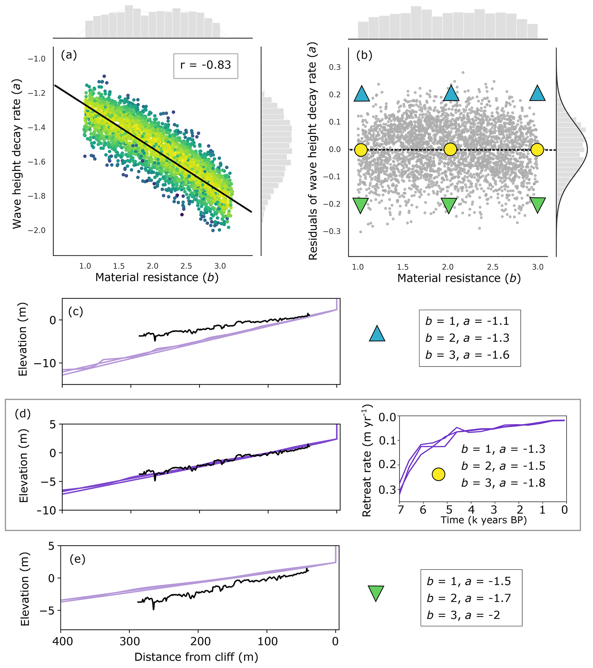
Figure 12(a) Objective function space of accepted samples from the MCMC analysis for material resistance (b) and wave height decay rate (a) parameters for Bideford. A linear regression calculation was performed and is shown along with the r value of −0.83. Histograms on either axis show the distribution of accepted sample points. (b) Residual plot from the regression line shown in (a). Yellow circles plotted along the regression line in (b) correspond to model outputs shown in (d) that show the best-fit to the measured topographic profile. Green triangles pointing upwards (b) are plotted +0.2 from the regression line and correspond to model outputs shown in (c). Green triangles pointing downwards (b) are plotted −0.2 from the regression line and correspond to model outputs shown in (e).
The objective function space for wave height decay rate (a) and material resistance (b) reveals a trade-off relationship between the two functions. A linear regression analysis was performed and highlights a finite range of linearly related a and b values that can produce a well-matched topographic profile and resultant 10Be concentration profile. The residuals of a, after fitting to the linear correlation in Fig. 12a, are shown (Fig. 12b). Nevertheless, the relationship between a and b is not as straightforward as saying faster wave height needs to be compensated for by a lower material resistance. Varying the wave height decay rate (a) changes the erosive energy distribution across the shore platform, and this ultimately influences the potential erosion achieved by waves. When waves dissipate energy too quickly (a is increased), erosion of the outer part of the platform is increased and less erosion is achieved towards the cliff base. As a result, modelled topographic profiles become too steep to match the gradient of the shore platform measured at Bideford (Fig. 12c). In contrast, when waves dissipate too slowly (a is decreased) and waves dissipate energy across a wider distance of the shore platform, erosion is increased further inshore and overall erosion across the shore platform is increased. The gradient of the modelled topographic profiles becomes less than 0.02 measured at the Bideford shore platform (Fig. 12e). Here we demonstrate the twofold impact of varying wave height decay rate: (1) increasing the distance across which waves break increases the amount of energy made available for erosion, and (2) varying the rate of wave dissipation affects the spatial distribution of erosion across the shore platform. The observed range of residuals across the regression and the resultant model outputs highlights the narrow uncertainty of y required to produce a matching topographic and 10Be concentration profile.
In order for an MCMC analysis to produce effective posterior distributions, the optimisation method requires free parameters to be independent of each other. As a result of the correlation revealed between a and b parameters, the high confidence placed on a values (Fig. 12) is not reflected by the posterior distributions produced from the MCMC results (Table 3). Wide posterior distributions of the accepted samples (axis histograms in Fig. 12a) produce large uncertainty for final MCMC results. We argue that propagating MCMC uncertainties for a together with the uncertainty for b produces unrealistic errors in model outputs, specifically seen in the large range of shore platform gradients. Consequently, the uncertainty in final model outputs (Figs. 6 and 7) is constructed by plotting the model result of the median and 16 %–84 % confidence range for each parameter against the median result for the other two parameters.
Comparisons between the two sites further support our observations of the relationship between material resistance (b) and wave height decay rate (a). The platform gradient at Scalby is shallower compared to Bideford, and best-fit results for a show that wave dissipation needs to be slower to match the topographic profile (Fig. 10). Best-fit a values are constrained by the lowest bound of a for Scalby with a limits informed by field-based studies (Ogawa et al., 2011). For Scalby, this either means (1) overall wave erosion needs to be greater, or (2) wave erosion needs to be more evenly distributed across the shore platform compared to Bideford. Furthermore, Scalby is located at a meso-tidal coastline with mean spring tidal ranges of 4.6 m, and studies have previously commented on the positive correlation observed between platform gradient and tidal range for real-world sites (e.g. Matsumoto et al., 2017). Future investigations into how b vs. a relationships may change as a function of platform gradient and/or tidal range within this exploratory model that are informed with additional site-specific datasets are needed in order to further understand this model behaviour.
5.3 Equifinality in cliff retreat trajectories
Correlation between a and b parameters at Bideford also shows that a matching topographic profile can be produced across the full extent of material resistance (b), provided wave height decay rate (a) has adjusted accordingly (Fig. 12d). A greater material resistance (b) requires a greater wave force, i.e. smaller wave height decay rate (a), in order to erode an across-shore intertidal shore platform with the same geometric properties. Correlation between a and b demonstrates one potential source of equifinality in terms of endmember topographic and 10Be concentration profiles. To ensure we report accurate cliff retreat rates, we need to identify whether equifinal a and b combinations result in similar cliff retreat trajectories as well as the same endmember model topographic and 10Be concentration profiles. The magnitude of material resistance (b) across the regression has no effect on the final fit for the topographic profile (Fig. 12d). Most importantly, the resultant cliff retreat rates all show comparable trajectories and rates of cliff retreat across the late Holocene. Therefore, as long as the combination of a and b tracks the regression fitted to the accepted samples (Fig. 12a), we can have confidence that the most accurate retreat rates are reported.
5.4 Interpretation of best-fit parameter values
It is important to recognise that the best-fit lower wave height decay rates (a) found at Scalby, which results in a breaking wave force to be exerted over a greater distance across the platform surface, do not necessarily mean that wave energy is greater at Scalby than Bideford. Wave energy is abstractly defined in the coastal evolution model by an assailing wave force, and we have chosen to explore this in the MCMC analysis by varying the wave height decay rate (a). Our aim is not to quantify the wave force at real-world coastlines, but to determine the best combination of model parameters to match measured datasets in order to model cliff retreat over timescales much longer than information on wave conditions is available. Wave height attenuation length is dependent on other factors such as profile gradient and tidal range, which are site-dependant (Trenhaile, 2000). We also have very few constraints on if and how tidal range has changed across the past 8000 years, as this depends strongly on local and far-field bathymetry, as well as other uncertain climatic variables. Furthermore, wave height decay rate is further impacted by surface roughness (Poate et al., 2018), and this is not considered within our model simulations. For these reasons, using wave height decay rate to infer wave energy for a range of real-world sites is unachievable with our model, even with a rigorous optimisation method. Moreover, parameter correlation, which is seen particularly well in the relationship between material resistance (b) and wave height decay rate (a) (see Sect. 5.2), means that finding a single best-fit result for wave height decay rate (a) is problematic without isolated parameter investigations. Nevertheless, the relative importance of the parameters that control wave-driven erosion (a) and weathering-controlled erosion (c) can be considered. Because best-fit results at Bideford clearly show that negligible contributions of weathering are needed to produce the 10Be concentration profile, we can conclude that the evolution of cliff retreat at Bideford is likely dominated by wave-driven erosion. In contrast, modelled best-fit values of low to intermediate weathering rates at Scalby reveal a more complex interplay between wave-driven and weathering-controlled erosion.
Resultant equifinality in cliff retreat trajectories (Fig. 12) reveals that correlation does not prevent identification of consistent patterns in cliff retreat rate histories. In other words, the relative combinations of a, b, and c parameter values are able to capture the morphodynamics needed to model compatible rock coast evolutions at unique rock coast sites. Therefore, the abstract representation of wave force, weathering processes, and material resistance within the RPM does not inhibit the modelling of cliff retreat for real-world sites. Furthermore, consistent trends in past cliff retreat rates for all Pareto weighting sets (Fig. 5) that match the declining rate of RSL rise suggest that the influence of the RSL boundary condition dominates over individual parameter values.
In this study, we have developed a multi-objective optimisation approach to reconstruct the history of rock coast evolution through the combination of morphodynamic modelling and field observations. Our approach calibrates a coupled morphodynamic–cosmogenic radionuclide rock coast evolution model using observations of modern rock coast topography and measurements of in situ 10Be concentrations in the exposed bedrock. These developments are vital to enable application of a process-based model to real-world coast sites and quantify a time series of rock coast erosion and sea cliff retreat rates. Our results demonstrate the necessity for using multi-objective optimisation in order to limit model equifinality, in which similar topographies develop via differing evolutionary trajectories. Optimal parameter selection is used to minimise discrepancies between model simulations and measured topography, and 10Be concentrations can reveal the most likely history of rock coast development, including rates of shore platform lowering and cliff retreat.
The selection of free parameters within the model optimisation focuses on the efficacy of intertidal weathering and erosion processes relative to the resistance of bedrock. There is still equifinality in model outcomes for parameter combinations for which similar patterns of topographic development occur. More resistant bedrock combined with efficient weathering and/or erosion can result in development of a rock coast profile similar to that of a less resistant bedrock and less effective weathering and/or erosion. This parameter correlation can be reduced through multi-objective optimisation but ultimately does not prevent identifying consistent patterns in cliff retreat rates at specific rock coast sites.
Investigations into the Pareto set of optimised results show that best-fit results are consistent across a range of objective function weightings. These findings suggest that a single, equally weighted MCMC chain is sufficient to find an optimal set of input model parameters in order to constrain the cliff retreat rate history.
By applying rigorous optimisation methods, we demonstrate how an abstract, process-based model is capable of reproducing the rock coast profile development of real-world sites. Moreover, when coupled with a 10Be production model, equifinality is sufficiently constrained to reveal distinctive trends in long-term cliff retreat rates. Long-term cliff retreat rates of two UK rock coast sites both closely mirror the history of RSL change rates. This link between the rate of RSL rise and cliff retreat rates indicates that future accelerations in RSL rise associated with climate change will cause accelerations in cliff retreat rates, even at coastal sites that have been stable historically. We are only able to understand how cliff retreat responds to RSL by modelling the trajectory of cliff evolution across timescales that capture these changes in RSL rise.
The multi-objective statistical modelling approach developed and tested in our study highlights potential for future efforts to (1) reconstruct past rates and patterns of cliff retreat over timescales appropriate to the magnitude and frequency of erosion events at rock coast sites, (2) assess the relative importance of weathering and wave-driven erosion processes, and (3) forecast future erosion rates under different scenarios for RSL change as a result of climate change.
Input datasets can be found in the Supplement. Input data files, plotting scripts, code, and documentation can be found at https://doi.org/10.5281/zenodo.5645478 (Hurst et al., 2021).
The supplement related to this article is available online at: https://doi.org/10.5194/esurf-9-1505-2021-supplement.
JRS, MDH, MDP, and DHR designed the research and analysed the data; JRS, DHR, MDH, BGH, KMW, and AJS collected measured datasets; DHR, JRS, BGH, and AJS prepared samples in the laboratory; JRS developed the optimisation routine with support from MDH and MDP; KMW performed AMS measurements; JRS, MDH, DHR, and MDP wrote the paper.
The contact author has declared that neither they nor their co-authors have any competing interests.
Publisher's note: Copernicus Publications remains neutral with regard to jurisdictional claims in published maps and institutional affiliations.
We thank Michael Ellis for general and ongoing support with the project and editorial assistance. We would also like to thank Katy Barnhart for invaluable assistance with the Dakota software implementation and Geraldo Fiorini Neto for help with Dakota installation and testing. We also thank Sarah Bradley for providing RSL history data, which is an essential component to this project. We would like to thank Emily Gusterson and Jay Ward for support with field data collection. Finally, we would like to thank the reviewers, whose comments have greatly strengthened this paper.
This work was supported by a studentship from the Natural Environment Research Council (NERC) Science and Solutions for a Changing Planet Doctoral Training Partnership (DTP), with additional funding by the British Geological Survey (BGS) to Jennifer R. Shadrick. Dylan H. Rood received support of ANSTO Research Portal (grant no. 10955).
This paper was edited by Andreas Baas and reviewed by Vincent Regard and one anonymous referee.
Adams, B. M., Eldred, M. S., Geraci, G., Hooper, R. W., Jakeman, J. D., Maupin, K. A., Monschke, J. A., Rushdi, A. A., Stephens, J. A., Swiler, L. P., Wildey, T. M., Bohnhoff, W. J., Dalbey, K. R., and Ebeida, M. S.: Dakota, A Multilevel Parallel Object-Oriented Framework for Design Optimization, Parameter Estimation, Uncertainty Quantification, and Sensitivity Analysis: Version 6.10 User's Manual, 388, 2019.
Balco, G., Stone, J. O., Lifton, N. A., and Dunai, T. J.: A complete and easily accessible means of calculating surface exposure ages or erosion rates from 10Be and 26Al measurements, Quat. Geochronol., 3, 174–195, https://doi.org/10.1016/j.quageo.2007.12.001, 2008.
Barlow, J., Moore, R., and Gheorghiu, D. M.: Reconstructing the recent failure chronology of a multistage landslide complex using cosmogenic isotope concentrations: St Catherine's Point, UK, Geomorphology, 268, 288–295, https://doi.org/10.1016/j.geomorph.2016.06.021, 2016.
Barnhart, K. R., Glade, R. C., Shobe, C. M., and Tucker, G. E.: Terrainbento 1.0: a Python package for multi-model analysis in long-term drainage basin evolution, Geosci. Model Dev., 12, 1267–1297, https://doi.org/10.5194/gmd-12-1267-2019, 2019.
Barnhart, K. R., Tucker, G. E., Doty, S. G., Shobe, C. M., Glade, R. C., Rossi, M. W., and Hill, M. C.: Inverting Topography for Landscape Evolution Model Process Representation: 2. Calibration and Validation, J. Geophys. Res.-Earth, 125, e2018JF004963, https://doi.org/10.1029/2018JF004963, 2020.
Bradley, S. L., Milne, G. A., Shennan, I., and Edwards, R.: An improved glacial isostatic adjustment model for the British Isles, J. Quat. Sci., 26, 541–552, https://doi.org/10.1002/jqs.1481, 2011.
Braucher, R., Bourlès, D., Merchel, S., Vidal Romani, J., Fernadez-Mosquera, D., Marti, K., Léanni, L., Chauvet, F., Arnold, M., Aumaître, G., and Keddadouche, K.: Determination of muon attenuation lengths in depth profiles from in situ produced cosmogenic nuclides, Nucl. Instrum. Meth. B, 294, 484–490, https://doi.org/10.1016/j.nimb.2012.05.023, 2013.
Brooks, S. M. and Spencer, T.: Temporal and spatial variations in recession rates and sediment release from soft rock cliffs, Suffolk coast, UK, Geomorphology, 2010.
Buchanan, D. H., Naylor, L. A., Hurst, M. D., and Stephenson, W. J.: Erosion of rocky shore platforms by block detachment from layered stratigraphy, Earth Surf. Proc. Land., 45, 1028–1037, https://doi.org/10.1002/esp.4797, 2020.
Choi, K. H., Seong, Y. B., Jung, P. M., and Lee, S. Y.: Using Cosmogenic 10Be Dating to Unravel the Antiquity of a Rocky Shore Platform on the West Coast of Korea, J. Coast. Res., 28, 641–657, https://doi.org/10.2112/JCOASTRES-D-11-00087.1, 2012.
Coombes, M. A.: Chapter 5 The rock coast of the British Isles: weathering and biogenic processes, Geo. Soc. Mem., 40, 57–76, https://doi.org/10.1144/M40.5, 2014.
Dornbusch, U., Robinson, D. A., Moses, C. A., and Williams, R. B. G.: Temporal and spatial variations of chalk cliff retreat in East Sussex, 1873 to 2001, Mar. Geol., 249, 271–282, https://doi.org/10.1016/j.margeo.2007.12.005, 2008.
Duguet, T., Duperret, A., Costa, S., Regard, V., and Maillet, G.: Coastal chalk cliff retreat rates during the Holocene, inferred from submarine platform morphology and cosmogenic exposure along the Normandy coast (NW France), Mar. Geol., 433, 106405, https://doi.org/10.1016/j.margeo.2020.106405, 2021.
Edmonds, E. A., Williams, B. J., and Taylor, R. T.: Geology of Bideford and Lundy Island, Institute of Geological Sciences, Natural Environment Research Council, London, 1979.
Estacio-Hiroms, K. C., Prudencio, E. E., Malaya, N. P., Vohra, M., and McDougall, D.: The QUESO Library, User's Manual, ArXiv, 161107521, Stat., 2016.
Gelman, A., Gilks, W. R., and Roberts, G. O.: Weak convergence and optimal scaling of random walk Metropolis algorithms, Ann. Appl. Probab., 7, 110–120, https://doi.org/10.1214/aoap/1034625254, 1997.
Gosse, J. C. and Phillips, F. M.: Terrestrial in situ cosmogenic nuclides: theory and application, Quaternary Sci. Rev., 20, 1475–1560, https://doi.org/10.1016/S0277-3791(00)00171-2, 2001.
Hastings, W. K.: Monte Carlo sampling methods using Markov chains and their applications, Biometrika, 57, 97–109, https://doi.org/10.1093/biomet/57.1.97, 1970.
Hurst, M., Matsumoto, H., Shadrick, J. R., Rood, D. H., and Dickson, M. E.: mdhurst1/Rocky-Profile-Model: RPM-CRN with Dakota Implementation v1.0 (RPMV1.0), Zenodo [code], https://doi.org/10.5281/zenodo.5645478, 2021.
Hurst, M. D., Rood, D. H., Ellis, M. A., Anderson, R. S., and Dornbusch, U.: Recent acceleration in coastal cliff retreat rates on the south coast of Great Britain, P. Natl. Acad. Sci. USA, 113, 13336–13341, https://doi.org/10.1073/pnas.1613044113, 2016.
Hurst, M. D., Rood, D. H., and Ellis, M. A.: Controls on the distribution of cosmogenic 10Be across shore platforms, Earth Surf. Dynam., 5, 67–84, https://doi.org/10.5194/esurf-5-67-2017, 2017.
Kennedy, D. M., Stephenson, W. J., and Naylor, L. A.: Chapter 1 Introduction to the rock coasts of the world, Geo. Soc. Mem., 40, 1–5, https://doi.org/10.1144/M40.1, 2014.
Kennedy, M. C. and O'Hagan, A.: Bayesian calibration of computer models, J. R. Stat. Soc. B, 63, 425–464, https://doi.org/10.1111/1467-9868.00294, 2001.
Limber, P. W. and Murray, A. B.: Beach and sea-cliff dynamics as a driver of long-term rocky coastline evolution and stability, Geology, 39, 1147–1150, https://doi.org/10.1130/G32315.1, 2011.
Masteller, C., Hovius, N., Thomspon, C., Vann-Jones, E., Woo, H. B., Adams, P., Dickson, M., Young, A., and Rosser, N.: Exploring the interplay of wave climate, vertical land motion, and rocky coast evolution, EGU General Assembly 2020, Online, 4–8 May 2020, EGU2020-12680, https://doi.org/10.5194/egusphere-egu2020-12680, 2020.
Matsumoto, H., Dickson, M. E., and Kench, P. S.: An exploratory numerical model of rocky shore profile evolution, Geomorphology, 268, 98–109, https://doi.org/10.1016/j.geomorph.2016.05.017, 2016.
Matsumoto, H., Dickson, M. E., and Masselink, G.: Systematic analysis of rocky shore platform morphology at large spatial scale using LiDAR-derived digital elevation models, Geomorphology, 286, 45–57, https://doi.org/10.1016/j.geomorph.2017.03.011, 2017.
Matsumoto, H., Dickson, M. E., and Kench, P. S.: Modelling the relative dominance of wave erosion and weathering processes in shore platform development in micro- to mega-tidal settings, Earth Surf. Proc. Land., 43, 2642–2653, https://doi.org/10.1002/esp.4422, 2018.
Metropolis, N., Rosenbluth, A. W., Rosenbluth, M. N., Teller, A. H., and Teller, E.: Equation of State Calculations by Fast Computing Machines, J. Chem. Phys., 21, 1087–1092, https://doi.org/10.1063/1.1699114, 1953.
Moses, C. A.: Chapter 4 The rock coast of the British Isles: shore platforms, Geo. Soc. Mem., 40, 39–56, https://doi.org/10.1144/M40.4, 2014.
Mudd, S. M., Harel, M.-A., Hurst, M. D., Grieve, S. W. D., and Marrero, S. M.: The CAIRN method: automated, reproducible calculation of catchment-averaged denudation rates from cosmogenic nuclide concentrations, Earth Surf. Dynam., 4, 655–674, https://doi.org/10.5194/esurf-4-655-2016, 2016.
National Tidal and Sea Level Facility: https://www.ntslf.org/ (last access: 29 November 21), last modified: 27 November 2021.
Naylor, L. A. and Stephenson, W. J.: On the role of discontinuities in mediating shore platform erosion, Geomorphology, 114, 89–100, https://doi.org/10.1016/j.geomorph.2008.12.024, 2010.
Nishiizumi, K., Imamura, M., Caffee, M. W., Southon, J. R., Finkel, R. C., and McAninch, J.: Absolute calibration of 10Be AMS standards, Nucl. Instrum. Meth. B, 258, 403–413, https://doi.org/10.1016/j.nimb.2007.01.297, 2007.
Ogawa, H., Dickson, M. E., and Kench, P. S.: Wave transformation on a sub-horizontal shore platform, Tatapouri, North Island, New Zealand, Cont. Shelf Res., 31, 1409–1419, https://doi.org/10.1016/j.csr.2011.05.006, 2011.
Payo, A., Hall, J. W., Dickson, M. E., and Walkden, M. J. A.: Feedback structure of cliff and shore platform morphodynamics, J. Coast. Conserv., 19, 847–859, https://doi.org/10.1007/s11852-014-0342-z, 2015.
Poate, T., Masselink, G., Austin, M. J., Dickson, M., and McCall, R.: The Role of Bed Roughness in Wave Transformation Across Sloping Rock Shore Platforms, J. Geophys. Res.-Earth, 123, 97–123, https://doi.org/10.1002/2017JF004277, 2018.
Porter, N. J., Trenhaile, A. S., Prestanski, K., and Kanyaya, J. I.: Patterns of surface downwearing on shore platforms in eastern Canada, Earth Surf. Proc. Land., 35, 1793–1810, https://doi.org/10.1002/esp.2018, 2010.
Prémaillon, M., Regard, V., Dewez, T. J. B., and Auda, Y.: GlobR2C2 (Global Recession Rates of Coastal Cliffs): a global relational database to investigate coastal rocky cliff erosion rate variations, Earth Surf. Dynam., 6, 651–668, https://doi.org/10.5194/esurf-6-651-2018, 2018.
Raimbault, C., Duperret, A., Regard, V., Molliex, S., Wyns, R., Authemayou, C., and Le Gall, B.: Quaternary geomorphological evolution of a granitic shore platform constrained by in situ 10Be concentrations, Penmarc'h, SW Brittany, France, Mar. Geol., 395, 33–47, https://doi.org/10.1016/j.margeo.2017.09.011, 2018.
Recorbet, F., Rochette, P., Braucher, R., Bourlès, D., Benedetti, L., Hantz, D., and Finkel, R. C.: Evidence for active retreat of a coastal cliff between 3.5 and 12 ka in Cassis (South East France), Geomorphology, 115, 1–10, https://doi.org/10.1016/j.geomorph.2009.04.023, 2010.
Regard, V., Dewez, T., Bourlès, D. L., Anderson, R. S., Duperret, A., Costa, S., Leanni, L., Lasseur, E., Pedoja, K., and Maillet, G. M.: Late Holocene seacliff retreat recorded by 10Be profiles across a coastal platform: Theory and example from the English Channel, Quat. Geochronol., 11, 87–97, https://doi.org/10.1016/j.quageo.2012.02.027, 2012.
Riding, J. B. and Wright, J. K.: Palynostratigraphy of the Scalby Formation (Middle Jurassic) of the Cleveland basin, north-east Yorkshire, P. Yorks. Geol. Soc., 47, 349–354, 1989.
Rogers, H. E., Swanson, T. W., and Stone, J. O.: Long-term shoreline retreat rates on Whidbey Island, Washington, USA, Quaternary Res., 78, 315–322, https://doi.org/10.1016/j.yqres.2012.06.001, 2012.
Stephenson, W. J., Kirk, R. M., and Hemmingsen, M. A.: Forty three years of micro-erosion meter monitoring of erosion rates on shore platforms at Kaikōura Peninsula, South Island, New Zealand, Geomorphology, 344, 1–9, https://doi.org/10.1016/j.geomorph.2019.07.012, 2019.
Sunamura, T.: Geomorphology of rocky coasts, vol. 302, Wiley, Chichester, 1992.
Sunamura, T.: Rocky coast processes: with special reference to the recession of soft rock cliffs, P. Jpn. Acad. B-Phys., 91, 481–500, https://doi.org/10.2183/pjab.91.481, 2015.
Swirad, Z. M., Rosser, N. J., and Brain, M. J.: Identifying mechanisms of shore platform erosion using Structure-from-Motion (SfM) photogrammetry, Earth Surf. Proc. Land., 44, 1542–1558, https://doi.org/10.1002/esp.4591, 2019.
Swirad, Z. M., Rosser, N. J., Brain, M. J., Rood, D. H., Hurst, M. D., Wilcken, K. M., and Barlow, J.: Cosmogenic exposure dating reveals limited long-term variability in erosion of a rocky coastline, Nat. Commun., 11, 3804, https://doi.org/10.1038/s41467-020-17611-9, 2020.
Thompson, C. F., Young, A. P., and Dickson, M. E.: Wave impacts on coastal cliffs: Do bigger waves drive greater ground motion?, Earth Surf. Proc. Land., 44, 2849–2860, https://doi.org/10.1002/esp.4712, 2019.
Trenhaile, A. S.: Modeling the development of wave-cut shore platforms, Mar. Geol., 166, 163–178, https://doi.org/10.1016/S0025-3227(00)00013-X, 2000.
Trenhaile, A. S.: Modeling the role of weathering in shore platform development, Geomorphology, 94, 24–39, https://doi.org/10.1016/j.geomorph.2007.04.002, 2008a.
Trenhaile, A. S.: The development of subhorizontal shore platforms by waves and weathering in microtidal environments, Z. Geomorphol., 52, 105–124, https://doi.org/10.1127/0372-8854/2008/0052-0105, 2008b.
Trenhaile, A. S.: Chapter 2 Climate change and its impact on rock coasts, Geo. Soc. Mem., 40, 7–17, https://doi.org/10.1144/M40.2, 2014.
Trenhaile, A. S.: Shore platform erosion and evolution: Implications for cosmogenic nuclide analysis, Mar. Geol., 403, 80–92, https://doi.org/10.1016/j.margeo.2018.05.005, 2018.
Walkden, M. J. A. and Hall, J. W.: A predictive Mesoscale model of the erosion and profile development of soft rock shores, Coast. Eng., 52, 535–563, https://doi.org/10.1016/j.coastaleng.2005.02.005, 2005.
Wilcken, K. M., Fink, D., Hotchkis, M. A. C., Garton, D., Button, D., Mann, M., Kitchen, R., Hauser, T., and O'Connor, A.: Accelerator Mass Spectrometry on SIRIUS: New 6MV spectrometer at ANSTO, Nucl. Instrum. Meth. B, 406, 278–282, https://doi.org/10.1016/j.nimb.2017.01.003, 2017.
Yuan, R., Kennedy, D. M., Stephenson, W. J., and Finlayson, B. L.: The multidecadal spatial pattern of erosion on sandstone shore platforms in south-eastern Australia, Geomorphology, 371, 107437, https://doi.org/10.1016/j.geomorph.2020.107437, 2020.