the Creative Commons Attribution 4.0 License.
the Creative Commons Attribution 4.0 License.
 | 09 Mar 2021
Growing topography due to contrasting rock types in a tectonically dead landscape
Cristina Persano
Martin D. Hurst
Paul Bishop
Derek Fabel
Many mountain ranges survive in a phase of erosional decay for millions of years following the cessation of tectonic activity. Landscape dynamics in these post-orogenic settings have long puzzled geologists due to the expectation that topographic relief should decline with time. Our understanding of how denudation rates, crustal dynamics, bedrock erodibility, climate, and mantle-driven processes interact to dictate the persistence of relief in the absence of ongoing tectonics is incomplete. Here we explore how lateral variations in rock type, ranging from resistant quartzites to less resistant schists and phyllites, and up to the least resistant gneisses and granitic rocks, have affected rates and patterns of denudation and topographic forms in a humid subtropical, high-relief post-orogenic landscape in Brazil where active tectonics ended hundreds of millions of years ago. We show that catchment-averaged denudation rates are negatively correlated with mean values of topographic relief, channel steepness and modern precipitation rates. Denudation instead correlates with inferred bedrock strength, with resistant rocks denuding more slowly relative to more erodible rock units, and the efficiency of fluvial erosion varies primarily due to these bedrock differences. Variations in erodibility continue to drive contrasts in rates of denudation in a tectonically inactive landscape evolving for hundreds of millions of years, suggesting that equilibrium is not a natural attractor state and that relief continues to grow through time. Over the long timescales of post-orogenic development, exposure at the surface of rock types with differential erodibility can become a dominant control on landscape dynamics by producing spatial variations in geomorphic processes and rates, promoting the survival of relief and determining spatial differences in erosional response timescales long after cessation of mountain building.
- Article
(11488 KB) - Full-text XML
-
Supplement
(6661 KB) - BibTeX
- EndNote


The question of how landscapes evolve in the aftermath of mountain building has intrigued geomorphologists since the early stages of the discipline, and classic concepts such as the cycle of erosion (Davis, 1899) and dynamic equilibrium landforms (Hack, 1960) were defined in the context of these post-orogenic landscapes (Bishop, 2007). In particular, reasons for the persistence of high topographic relief in ancient mountain belts for many millions of years after crustal thickening remain enigmatic. We know with a reasonable degree of certainty that net erosion in these landscapes and the resulting rebound of the underlying lithosphere by isostasy are central mechanisms controlling the extended longevity of post-orogenic landforms (Gilchrist and Summerfield, 1990; Bishop and Brown, 1992; Bishop, 2007). However, a range of other factors and interactions play essential roles in the post-orogenic evolution of ancient landscapes, including variations in bedrock incision dynamics (e.g. Baldwin et al., 2003; Egholm et al., 2013), mantle flow dynamics and their influence on the overlying crust (e.g. Gallen et al., 2013; Liu, 2014), vertical and lateral variations in bedrock erodibility (e.g. Twidale, 1976; Bishop and Goldrick, 2010; Gallen, 2018; Bernard et al., 2019; Vasconcelos et al., 2019), densification of the lower crust and resulting reduction of the buoyancy of the lithosphere (e.g. Blackburn et al., 2018), and tectonic uplift in response to far-field stresses (e.g. Hack, 1982; Quigley et al., 2007).
Examples of ancient mountain belts marked by high elevations and steep slopes include the Appalachian Mountains, several mountain ranges in southeastern Brazil, the Cape Mountains, parts of the East Australian Highlands, the Ural Mountains, the Caledonides, the Western Ghats, and the Sri Lanka orogen (Fig. 1). These high-relief post-orogenic settings are associated with different climate conditions, tectonic histories, effective elastic thicknesses of the lithosphere, and geological architectures. For instance, some of these ancient mountain belts are located in a passive margin context, whereas others are located in the deep interior of the continents (Fig. 1). Yet they share common geomorphic characteristics, such as overall low rates of denudation (e.g. Harel et al., 2016), relative Cenozoic tectonic quiescence (e.g. Twidale, 1976; Mandal et al., 2015), exposure of a variety of resistant and more erodible lithologies (e.g. Bishop and Goldrick, 2010; Gallen, 2018; Vasconcelos et al., 2019), peak elevations that may exceed 2000 m, and average elevations commonly higher than 1000 m (e.g. von Blanckenburg et al., 2004; Gallen et al., 2013; Scharf et al., 2013).

Figure 1Global elevation and striking examples of high-relief ancient mountain belts. Post-orogenic settings highlighted by yellow ellipses: (1) the Appalachian Mountains, (2) SE Australia, (3) SE Brazil, (4) the Cape Mountains, (5) the Ural Mountains, (6) the Scandinavian Caledonides, (7) the Guyana Shield, (8) the Western Ghats, and (9) the Sri Lanka orogen. Dotted white lines represent high-elevation passive margins. We extracted elevation data from the US Geological Survey's (USGS) Global Multi-resolution Terrain Elevation data 2010 (GMTED2010).
Early landscape evolution schemes (e.g. Davis, 1899) and quantitative estimates of post-orogenic relief reduction (e.g. Ahnert, 1970; Baldwin et al., 2003; Egholm et al., 2013) predict a progressive decay in both topographic relief and denudation rates, with residual post-orogenic landforms marked by featureless topography reminiscent of peneplains after hundreds of millions of years of ongoing denudation. More recently, a range of geomorphic and thermochronologic data indicates that topographic evolution in ancient mountain chains may be more dynamic than otherwise expected, with different types of forcing (e.g. tectonic, climatic, lithologic, mantle-driven) affecting at least some of these landscapes in post-orogenic times (e.g. Pazzaglia and Brandon, 1996; Quigley et al., 2007; Gallen et al., 2013; Tucker and van der Beek, 2013; Liu, 2014; Gallen, 2018). Our current knowledge on post-orogenic landscape evolution suffers from an incomplete understanding of how and to what extent different types of forcing may act in concert in driving the development of decaying mountain belts that are evolving over timescales of millions of years (Bishop, 2007; Tucker and van der Beek, 2013).
Most post-orogenic landscapes are characterised by complex and spatially variable lithology, often including crystalline rocks, different types of deformed metasediments and sedimentary covers, and volcanic units (e.g. Dorr, 1969; Bierman and Caffe, 2001; Barreto et al., 2013; Gallen et al., 2013; Mandal et al., 2015). Spatial variations in rock type have long been identified as a critical factor in post-orogenic development as they determine spatial heterogeneities in erodibility (e.g. Hack, 1960; Dorr, 1969; Hack, 1975; Twidale, 1976; Mills, 2003; Bishop and Goldrick, 2010; Gallen, 2018; Bernard et al., 2019; Vasconcelos et al., 2019; Zondervan et al., 2020a). In particular, correlations between rock type and topographic forms were observed in post-orogenic landscapes, with high topographic relief and steep channel reaches associated with resistant rocks (e.g. Hack, 1960, 1975; Twidale, 1976; Mills, 2003; Spotila et al., 2015; Gallen, 2018). These observations were interpreted, in several cases, as equilibrium adjustments where spatial variations in rock strength are balanced by variations in topographic relief so that everywhere is eroding at the same rate, with the corollary that topographic forms are constant through time in a “topographic equilibrium” likely driven by isostatic uplift (e.g. Hack, 1960; Matmon et al., 2003; Scharf et al., 2013; Mandal et al., 2015). In contrast, recent modelling studies indicate that exposure at the surface of rock units with substantial differences in rock strength dictate complex patterns of denudation, with significant spatial and temporal variations in denudation rates and possibly the persistence of non-steady-state conditions as long as different rock units are exposed (Forte et al., 2016; Perne et al., 2017). Post-orogenic settings are well suited as natural laboratories to explore further the role of spatial variations in lithology in landscape evolution, as these are lithologically heterogeneous landscapes that last experienced major active rock uplift tens to hundreds of millions of years ago (Bishop, 2007). Nevertheless, few studies have directly explored the spatial variability of denudation rates in post-orogenic settings as a function of the full spectrum of variations in underlying lithology and topographic relief in these landscapes.
Here, we investigated how denudation rates vary spatially in a humid subtropical, high-relief post-orogenic area in Brazil where the last phase of tectonic activity ended ∼500–450 Ma and explored the relationships between denudation rates and topographic relief, channel steepness, precipitation rates, and rock type. Denudation rates were measured using 10Be concentrations in fluvial sediments from catchments spanning the range of topographic relief and bedrock lithologies in the study area.
The study area is the Quadrilátero Ferrífero (Brazil), one of Brazil's highest elevation areas, with a peak elevation of 2076 m, located in the continental interior ∼350 km away in a straight line from the Atlantic Ocean (Fig. 2). The name Quadrilátero Ferrífero (QF) translates as “Iron Quadrangle”, referring both to its vast iron ore reserves and the roughly rectangular alignment of its ridges (Dorr, 1969). Local relief can reach 1189 m over a 2 km diameter circular window (Fig. 2a). There is an abundance of mixed bedrock–alluvial channels that incise deeply into the most resistant rocks but are less incised where more erodible lithologies are exposed; everywhere, however, the slope is enough for the detrital material to be removed, as alluvium has not significantly accumulated in the study area (Dorr, 1969). Normalised channel steepness, which is a metric for channel slope normalised to catchment size according to an assumed channel profile concavity, differs over 3 orders of magnitude (Fig. 2c). The regional climate ranges from Cwa to Cwb in Köppen–Geiger's classification (Alvares et al., 2013). Mean annual precipitation varies from 1356 to 1729 mm yr−1 (Fick and Hijmans, 2017), and the mean annual temperature is ∼20 ∘C (Dorr, 1969).
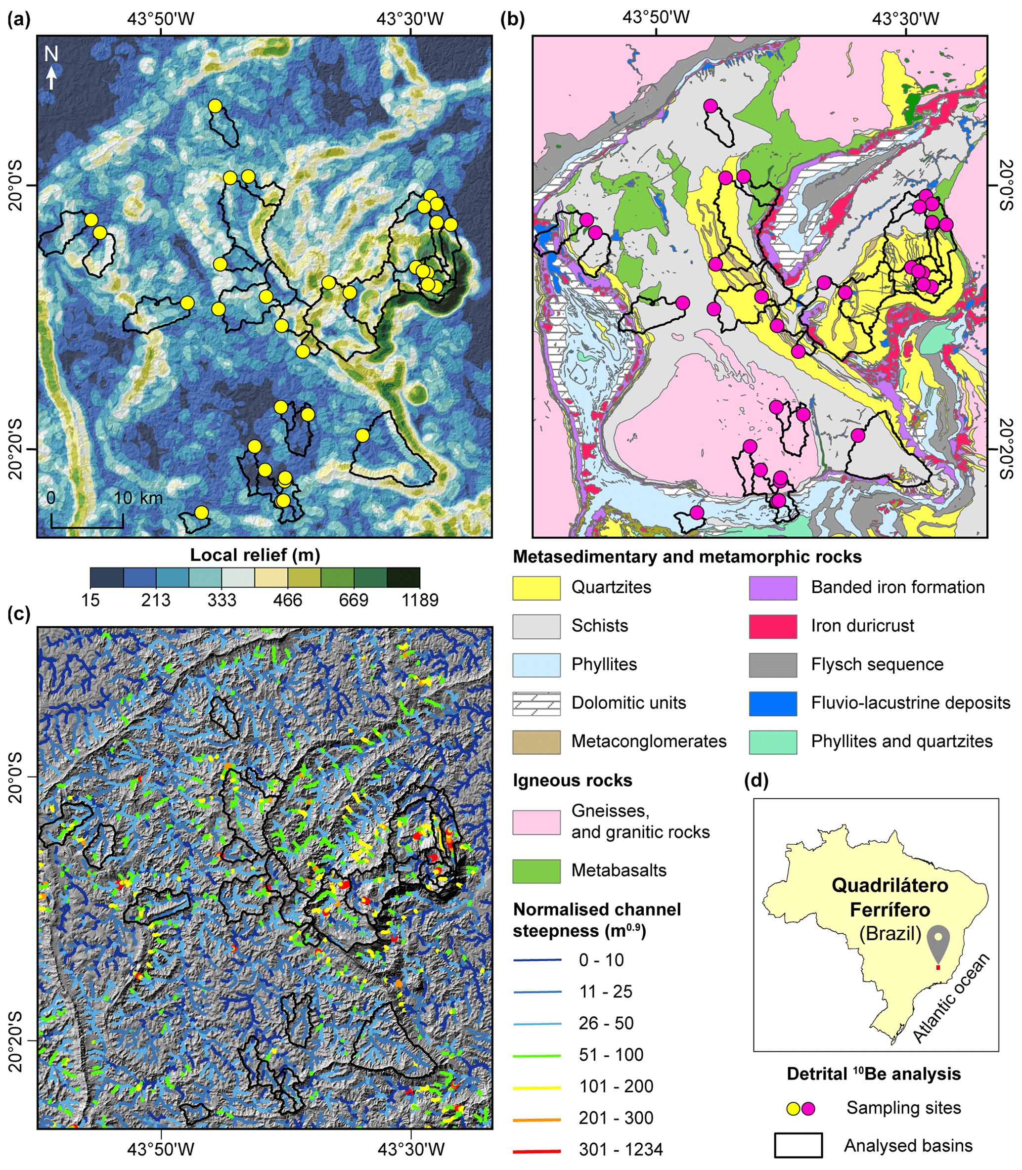
Figure 2The geomorphic context of the Quadrilátero Ferrífero, Brazil. (a) Map of local topographic relief (extracted using a 2 km diameter window). (b) Simplified bedrock geology in the study area, comprising mostly steeply dipping (≥35∘) Archean and Paleoproterozoic sequences. (c) Map of normalised channel steepness (ksn) extracted using the segmentation method of Mudd et al. (2014), with θref of 0.45. Note that we used an area threshold of 1.0 km2 to extract the drainage network, and we did not show sampling sites in (c) for illustration purposes. (d) The location of the QF in Brazil, ∼350 km away (in a straight line) from the Atlantic Ocean.
Resistant and more erodible lithologies are exposed in a complex geological pattern (Fig. 2b) that reflects a polyphase deformation history, the last episode of which was ∼500–450 Ma (Dorr, 1969; Chemale et al., 1994; Alkmim and Marshak, 1998). Exposed lithologies comprise principally Archean and Paleoproterozoic sequences, usually metamorphosed and steeply dipping (≥35∘), including gneisses and granitic rocks, schists, phyllites, quartzites, metaconglomerates, metacarbonate rocks, metavolcanics, banded iron formations, and iron duricrusts (Dorr, 1969; Chemale et al., 1994; Alkmim and Marshak, 1998). An array of geochronological data imply that the current topography is long-lived. These data include a relatively large set of (U-Th)/He data (n=291) and cosmogenic 3He concentrations (n=71) in iron oxides showing mineral precipitation ages as old as 55 Ma (varying from 55.3±5.5 to 0.4±0.1 Ma) and exposure ages ranging from 10.9±1.2 to 0.2±0.1 Ma, with age versus elevation relationships suggesting older ages and a more extended history of exposure in iron duricrust-covered plateaus at higher elevations (Monteiro et al., 2014, 2018); dating of Mn oxide grains collected in nine weathering profiles in the QF (n=174 grains that produced reliable results) yielding ages ranging from 94.6±5.5 to 12.3±0.5 Ma that are predominantly distributed between 30–60 Ma (Spier et al., 2006; Vasconcelos and Carmo, 2018); and low denudation rates (<3 m Myr−1) implied by cosmogenic 3He and 10Be inventories (Salgado et al., 2008; Monteiro et al., 2018). However, some authors have hypothesised, based principally on the post-depositional deformation of Cenozoic sediments that fill small basins (Fig. S1 in the Supplement), that the eastern part of the QF was affected by Cenozoic tectonics (e.g. Sant'Anna et al., 1997).
3.1 Determination of denudation rates
We collected alluvial sand from the bed of 25 active channels for the determination of denudation rates from detrital 10Be concentrations. Sampling included catchments spanning the range of topographic relief in the QF (Fig. 2a) and the range of bedrock lithologies (Fig. 2b), from resistant quartzites to the least-resistant (under humid subtropical conditions) gneisses and granitic rocks. The sampled basins do not show evidence of deep-seated landslides, and there are no records of significant landslide activity in the study area (Dorr, 1969). Samples were prepared and analysed at SUERC (Scottish Universities Environmental Research Centre), Scotland, following standard procedures (Kohl and Nishiizumi, 1992); NIST SRM4325 was the 10Be standard. The resulting ratios for each sample were corrected for processed blank ratios (n=2), ranging between 0.2 % and 3.2 % of the sample ratios, with uncertainties propagated in quadrature (Balco et al., 2008).
Catchment-averaged denudation rates were derived from 10Be concentrations using the CRONUS online calculator v3.0 (Balco et al., 2008). We used the CAIRN method (Mudd et al., 2016) to quantify catchment-averaged pressure employing a pixel-by-pixel approach and recommended parameters (Mudd et al., 2016). We report denudation rates using the time-independent Lal/Stone scaling method (Lal, 1991; Stone, 2000) and assuming a standard bedrock density of 2.7 g cm−3 (e.g. von Blanckenburg et al., 2004; Mandal et al., 2015). We have not applied corrections for topographic shielding (DiBiase, 2018). We have also incorporated eight detrital 10Be-derived concentration measurements previously published for the QF (Salgado et al., 2008) in our dataset; however, we recalculated denudation rates using the method described above to ensure consistency (Table S1 in the Supplement).
3.2 Quantification of catchment-averaged geomorphic metrics
We used a 12 m TanDEM-X (TerraSAR-X add-on for Digital Elevation Measurement) digital elevation model (DEM) to extract the following topographic metrics: (i) local relief and (ii) normalised channel steepness. The WorldClim v2 dataset (Fick and Hijmans, 2017) was used to extract (iii) mean annual precipitation rates. These metrics have been demonstrated to play an essential role in revealing the pattern and style of landscape evolution in erosive settings (e.g. Ahnert, 1970; Montgomery and Brandon, 2002; DiBiase et al., 2010; Portenga and Bierman, 2011; Harel et al., 2016). Catchments were extracted from the DEM following standard hydrological routing procedures using sample locations as pour points. Catchment-averaged values for each metric were determined as the average of all local values within each catchment.
Various authors have observed empirically that channel slope (S) declines progressively as contributing drainage area (A) increases in the downstream direction of a channel profile, in a relationship that can be described by a power law (e.g. Flint, 1974):
where θ, termed the “channel concavity”, controls how rapidly channel slope decreases with increasing drainage area, and ks, referred to as the “channel steepness”, is a measure of channel steepness normalised by upstream drainage area, which has been demonstrated to correlate positively with denudation rates in different geomorphic conditions (e.g. DiBiase et al., 2010; Mandal et al., 2015; Harel et al., 2016). The parameters ks and θ covary, and this autocorrelation is corrected by defining a fixed reference concavity (θref), which is used to extract a normalised channel steepness (ksn) from the data (Kirby and Whipple, 2012).
Equation (1) can be used to derive estimates of ks and θ (or ksn) from regressions of log-transformed slope area data (Kirby and Whipple, 2012). Alternatively, one can extract ksn using an approach referred to as the integral method (Perron and Royden, 2013). For that, Eq. (1) is rearranged by replacing S with and separating these variables, where z is elevation and x is distance along the channel, which is then integrated in the upstream direction from an arbitrarily base level at xb, resulting in an equation for the elevation profile (e.g. Mudd et al., 2018):
where A0 is a reference drainage area that is inserted to make the area term dimensionless (Perron and Royden, 2013). One can then define a longitudinal coordinate chi (χ) with dimensions of length using (Perron and Royden, 2013; Mudd et al., 2014):
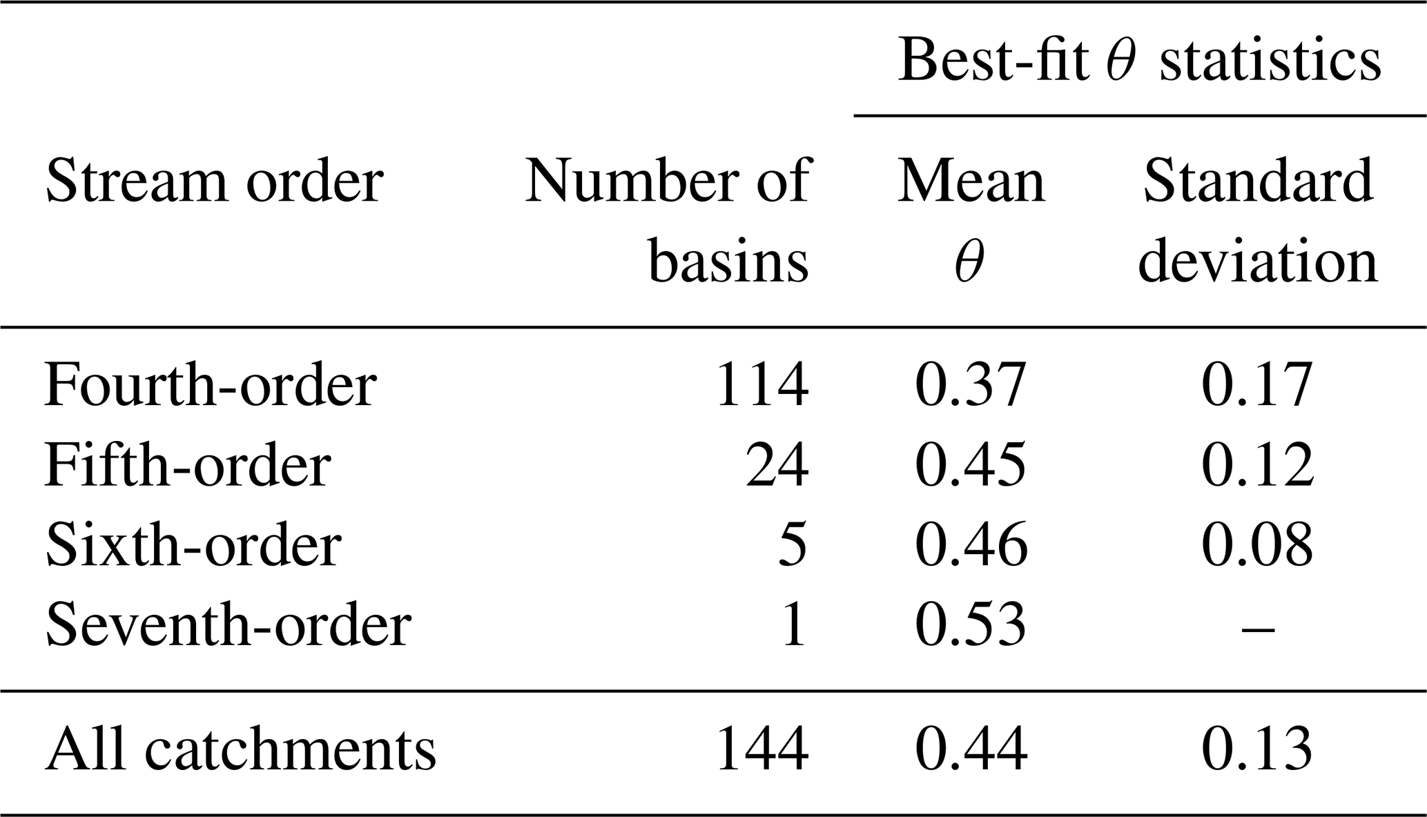
In the case of A0=1, the slope of a longitudinal profile in a z versus χ plot is the channel steepness (ks) or the normalised channel steepness (ksn) if the extraction is based on θref. We quantified ksn as the derivative of χ and z (e.g. Mudd et al., 2014) instead of using regressions of slope area data (e.g. DiBiase et al., 2010; Kirby and Whipple, 2012) because the integral method does not require estimating slope from the DEM, resulting in more precise ksn values (Perron and Royden, 2013). We estimated how θ varies over the study area based on the disorder method (Hergarten et al., 2016), which was carried out using routines developed by Mudd et al. (2018), to derive an optimal θ value for the entire landscape. The drainage network was extracted using an area threshold of 0.5 km2 (e.g. Beeson et al., 2017; Campforts et al., 2020), which is lower than the minimum drainage area among the catchments where we collected fluvial sediments (0.86 km2) and is a reasonable critical threshold for the study area (Fig. S2). We computed θ for all catchments of a stream order higher than the third order following Strahler (1957) (n=144), covering the entire study area; these catchments were extracted using code developed by Clubb et al. (2019). The mean θ for the QF (0.44; Table 1) is close to the frequently used value of 0.45 (e.g. Mandal et al., 2015); thus, we set 0.45 as the reference concavity from which we computed the normalised channel steepness employing the segmentation method of Mudd et al. (2014).
Table 1Variability in θ in the QF. Best-fit θ values were computed for all catchments of a stream order higher than the third order based on the disorder method (Hergarten et al., 2016) using code developed by Mudd et al. (2018).
We quantified local relief as the elevation range within a neighbourhood defined by a 2 km diameter circular window. The choice of the local relief window was based on sensitivity analysis (DiBiase et al., 2010). We compared the goodness-of-fit in bivariate regressions between average values of local relief (with window diameter varying from 0.5 to 5.0 km) and normalised channel steepness for every catchment in the study area with a stream order higher than the second order. In this situation, the local relief obtained using the 2 km diameter window exhibits the highest goodness-of-fit value (measured using the ordinary least squares method; Myers, 1990) with catchment-averaged normalised channel steepness (Fig. S3), and it is therefore the one that has been used throughout. Finally, we extracted mean annual precipitation rates from the 30 arcsec spatial resolution WorldClim v2 global monthly precipitation dataset for the years 1970 to 2000, which is based on raw weather station data and covariates from satellite sensors that were interpolated and combined, creating global climate surfaces (Fick and Hijmans, 2017).
3.3 Lithological strength and fluvial erosion efficiency in the QF
The QF is characterised by the presence of vast ore deposits, particularly gold, iron and manganese (Dorr, 1969; Lobato et al., 2001). The exploitation of these ore reserves has led to focused research, and the QF is the most systematically investigated geological domain in Brazil (Lobato et al., 2001). We extracted geological data from the “Projeto Geologia do Quadrilátero Ferrífero” dataset mapped at a scale of 1:25 000 (Lobato et al., 2005).
Rivers in the study area erode through a landscape marked by variations in rock type, including granitic, argillaceous, quartzose and carbonate rocks, as well as iron formations. These rock units are metamorphosed and steeply dipping as a result of QF's polyphase deformation history (Dorr, 1969; Chemale et al., 1994; Alkmim and Marshak, 1998). There is a clear consensus from geological research that the exposed lithologies have differential resistance to weathering and erosion, whereby quartzites, banded iron formations, and iron duricrusts comprise the most resistant lithologies; schists, phyllites, dolomitic units, and metavolcanics rocks are less resistant lithologies; and gneisses and granitic rocks are the least resistant rocks exposed in the QF (e.g. Dorr, 1969; Salgado et al., 2008; Monteiro et al., 2018; Vasconcelos and Carmo, 2018). Following the approach taken by previous studies (e.g. Lague et al., 2000; Korup, 2008; Jansen et al., 2010; Hurst et al., 2013), we assumed that such classification of rock strength as a function of rock type is valid, although we do not have rock strength measurements to support it. Given the humid subtropical condition of the QF, we expect differential resistance to reflect variations in the susceptibility to chemical weathering of the different rock units (Meybeck, 1987; White and Blum, 1995). For instance, gneisses and granitic rocks with an abundant presence of feldspars are readily weathered, whereas physically robust and chemically inert quartzites weather much more slowly via the intergranular solution of quartz (Dorr, 1969). In general in the study area, quartzites and banded iron formations form pronounced ridges and steep landforms with relatively unweathered outcrops compared to areas in gneisses and granitic rocks associated with broad lowlands that are deeply weathered, with regolith extending to depths of 50 m or more (e.g. Dorr, 1969; Salgado et al., 2008).
Theory and field observations demonstrate that rock strength influences long-term fluvial incision rates in erosive settings (e.g. Gilbert, 1877; Howard and Kerby, 1983; Stock and Montgomery, 1999; Whipple and Tucker, 1999; Jansen et al., 2010; Bursztyn et al., 2015) in concert with a number of other controls, including climate conditions and runoff efficiency, channel width scaling, extreme hydrologic events, and frequency of debris flow (e.g. Snyder et al., 2000; Whipple et al., 2000a; Kirby and Whipple, 2001; Duvall et al., 2004; Zondervan et al., 2020b). All of these factors are encapsulated in a dimensional coefficient of erosion efficiency (K) in the commonly used stream power model (Howard and Kerby, 1983):
where E is the long-term fluvial erosion; A is the upstream contributing drainage area; S is the local channel gradient; and m and n are positive exponents that depend on incision process, channel hydraulics, and rainfall variability (Whipple and Tucker, 1999).
Whereas most variables in the stream power model can be derived from DEM data, the fluvial erosion efficiency coefficient (K) cannot be measured directly, and thus the computing of K demands constraints on timing and/or rates of river evolution (Zondervan et al., 2020b). We have a limited understanding of how K varies in different geomorphic conditions and what controls its variability due to the few studies that derived absolute constraints on K and confounding between the multiple controls encoded in K (Snyder et al., 2000; Whipple et al., 2000a; Duvall et al., 2004; Harel et al., 2016; Zondervan et al., 2020b). More sophisticated versions of the stream power model may explicitly account for different controls in K (e.g. DiBiase and Whipple, 2011; Campforts et al., 2020; Zondervan et al., 2020b), yet such an approach requires specific data of an adequate resolution, such as river hydraulic geometry, rock strength measurements, and hydrological data to resolve spatial and temporal runoff variability, which are not readily available.
We computed catchment-averaged values of K for the QF using an approach similar to Gallen (2018) based on ksn and average erosion rates. Such an approach requires that spatial variability in long-term rock uplift over the study area is low, which is a reasonable assumption for the QF. Rearranging Eq. (4) to solve for channel slope can cast the stream power model in the same form as Eq. (1):
where
and thus
We extracted ksn using 0.45 as the reference concavity, which assuming m=0.45 and n=1 yields K values with units of m0.1 yr−1. We assumed that catchment-wide denudation rates derived from detrital 10Be concentrations are representative of long-term fluvial incision in the QF, considering that there are no records of the occurrence of deep-seated landslides (Dorr, 1969) and that sampled catchments are of a reasonable size. We calculated K assuming n=1 and n=2, which have been previously demonstrated as feasible values of n (Lague, 2014). In the study area, the range of precipitation is relatively low (from 1356 to 1729 mm yr−1), with areas of higher elevations principally underlain by resistant rocks receiving more precipitation than valley bottoms in more erodible rock units (Fig. S4), indicating opposing effects in K between inferred rock strength and precipitation rates. We explored how rock type and precipitation rates are linked to catchment-averaged values of K.
4.1 Catchment-averaged denudation rates in the QF
Catchment-averaged denudation rates in the study area range from 0.6±0.1 to 22.2±1.9 m Myr−1, with a regional mean denudation rate of 6.4 m Myr−1 (Fig. 3; Table S1). Denudation rates in the QF are thus comparable to or lower than previous estimates of denudation rates in other tectonically inactive, post-orogenic settings (e.g. Harel et al., 2016), including the Cape Mountains (e.g. Scharf et al., 2013), the Appalachian Mountains (e.g. Matmon et al., 2003), the Ozark dome (e.g. Beeson et al., 2017), the Sri Lankan uplands (e.g. von Blanckenburg et al., 2004) and the Western Ghats (e.g. Mandal et al., 2015). However, denudation rates are not uniformly low in the study area, varying by more than an order of magnitude (Fig. 3), from the slowly denuding catchments in the eastern part of the QF, where all catchments exhibit denudation rates lower than 3.5 m Myr−1, to the western part of the QF where catchments are eroding at higher rates up to 22.2±1.9 m Myr−1 (Fig. 3).
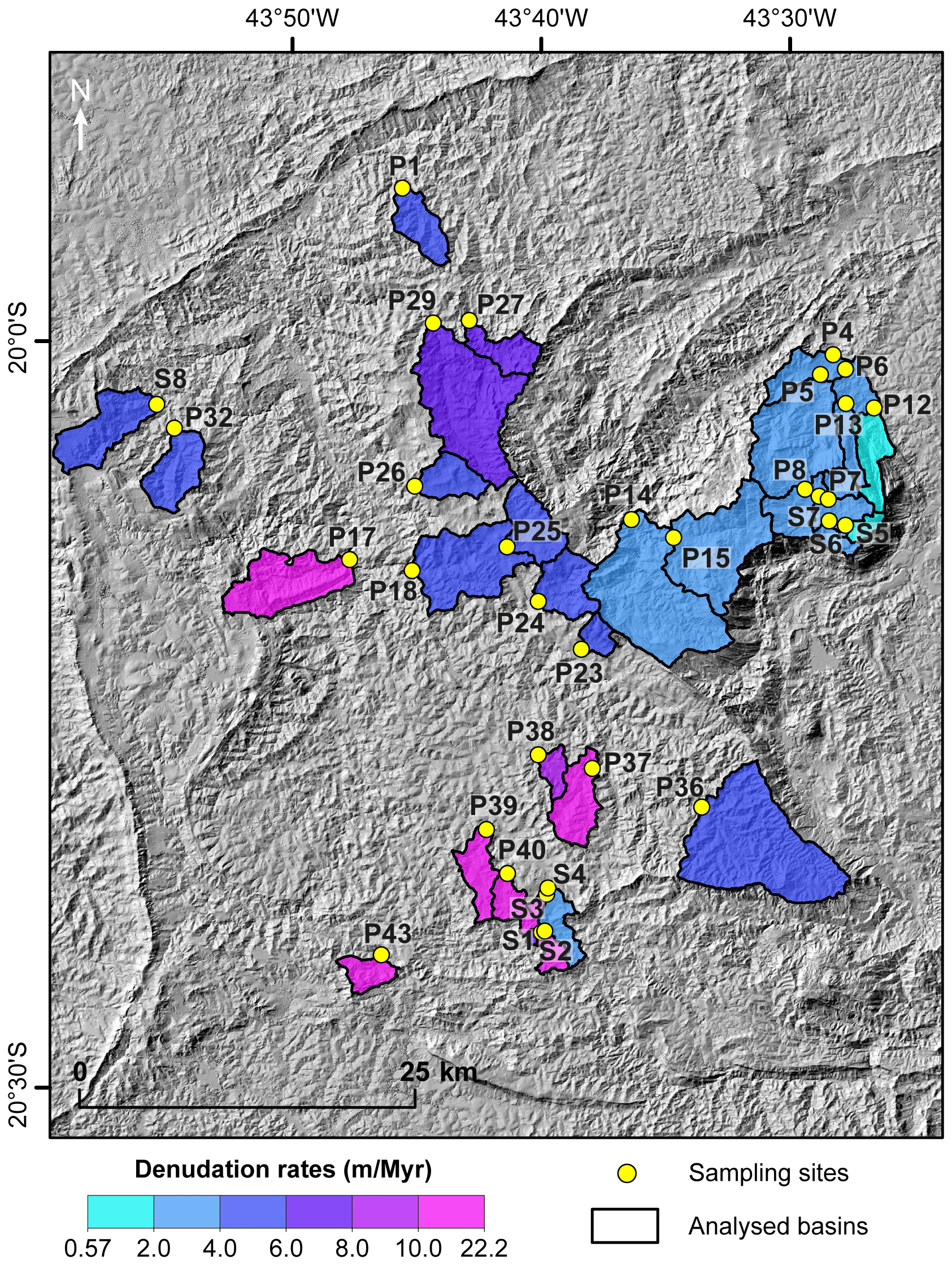
Figure 3Catchment-averaged denudation rates in the study area draped over a hillshade image. Note that we identify the 25 sampling sites of this study with “P” followed by a number, whereas we label the 8 sampling sites incorporated from Salgado et al. (2008) with “S” followed by a number. See Table S1 for 10Be analytical results and derived denudation rate data.
4.2 Links between topographic metrics, precipitation rates, rock type, and denudation rates
We find that catchment-averaged denudation rates are negatively correlated with mean values of local relief (Fig. 4a), contrary to the established understanding of links between denudation and topographic relief and the bulk of supporting empirical studies (e.g. Ahnert, 1970; Montgomery and Brandon, 2002; DiBiase et al., 2010; Harel et al., 2016). Similarly, catchment-averaged denudation rates are negatively correlated with mean values of normalised channel steepness (Fig. 4b), a parameter often used to infer denudation rates based on the empirical positive correlation between denudation and normalised channel steepness in tectonically active landscapes (e.g. DiBiase et al., 2010; Kirby and Whipple, 2012; Harel et al., 2016). We also find a negative relationship between catchment-averaged denudation rates and mean annual precipitation (Fig. 4c), contrary to the expectation that wetter climates drive more rapid denudation (e.g. Moon et al., 2011; Harel et al., 2016), and finally we find a weak correlation between catchment-averaged denudation rates and catchment area (Fig. S5). However, we observe that catchment-averaged denudation rates may increase together with mean values of topographic metrics and precipitation rates for individual rock types, although with such small sample sizes no such relationships are statistically significant at the α=0.05 level except for catchments in phyllites (Figs. 4 and S6).

Figure 4Links between denudation rates, geomorphic parameters, and rock type in the study area. Variations in catchment-averaged denudation rates with (a) mean local relief, (b) mean normalised channel steepness, (c) mean annual precipitation rates, and (d) percentage areal contribution of resistant rocks. Error bars on the y axis show measurement uncertainties in the nuclide concentration, as well as uncertainties related to the scaling method, and error bars on the x axis indicate the standard error of the mean. (e) Variations in catchment-averaged denudation rates per rock type, with the box on the left and raw data (diamonds) on the right. Box range represents the standard error of the mean, whiskers show the interval between the 10th and 90th percentiles of the data, white squares show mean values, and thick black lines exhibit median values. Mixed lithology refers to catchments where a single lithology does not account for ≥75 % of the catchment area.
Denudation rates can instead be linked to inferred rock strength (Fig. 4e). Catchments underlain by quartzites are associated with the slowest denudation rates (from 0.6±0.1 to 3.3±0.3 m Myr−1, with a mean of 2.2 m Myr−1). Catchments in mixed lithologies where ≥60 % of catchment area consists of resistant lithologies denude at slightly higher rates up to 3.5±0.3 m Myr−1 (with a mean of 2.6 m Myr−1). In contrast, catchments in less resistant schists or mixed lithologies with <60 % of resistant lithologies denude more rapidly. Finally, the low-relief catchments underlain by the least resistant (under humid subtropical climate conditions) gneisses and granitic rocks, as well as catchments dominated by phyllites, denude at higher rates of up to 22.2±1.9 m Myr−1. Similarly, we observe that a higher percentage contribution of resistant rocks in the catchment area (i.e. areas in quartzites and banded iron formations) determines lower rates of denudation (Fig. 4d).
The regional distribution of topographic metrics indicates a positive correlation between topography and inferred rock strength (Fig. 5). In this situation, the high end of the distribution of topographic metrics, as well as mean and median values, exhibits similar trends of high values for areas underlain by quartzites and banded iron formations; intermediate values for less resistant rock types such as metabasalts, schists, and phyllites; and low values for areas underlain by the least resistant basement rocks, which are also marked by lower variability in topography than areas dominated by resistant rocks. However, the low end of the distribution of topographic metrics shows comparably low values for every rock type, which indicates that subdued local relief and channel steepness occur on all lithologies. We also find positive relationships between catchment-averaged topographic relief and inferred rock strength (Fig. 5c). In particular, we observe that catchments in mixed lithologies where ≥60 % of catchment area consists of resistant lithologies exhibit substantially higher local relief than catchments in mixed lithologies with less than 60 % of resistant lithologies.
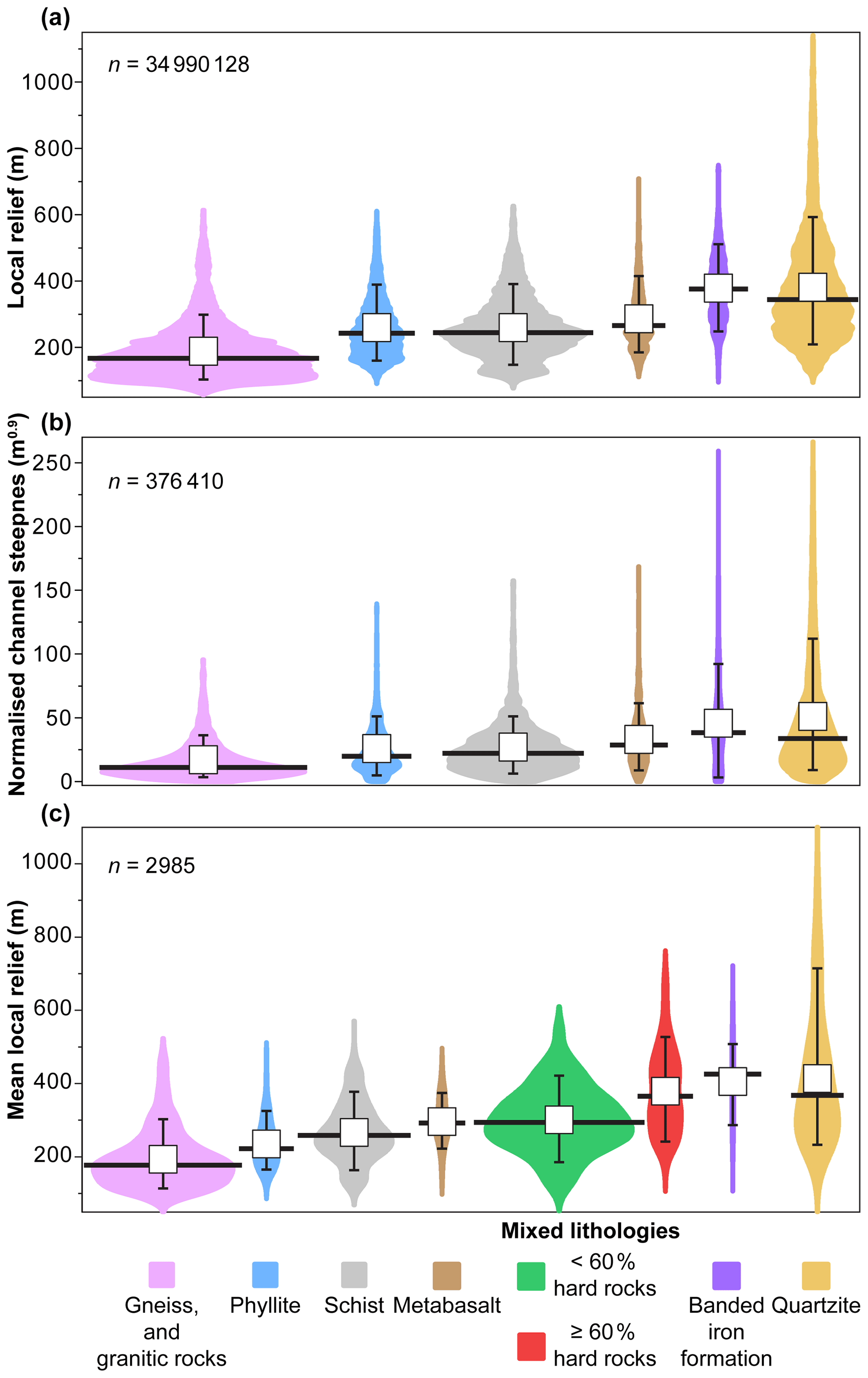
Figure 5Lithology controls topographic forms in the study area. Violin plots show the probability density (smoothed by a kernel density estimator), per rock type, of (a) local relief, (b) normalised channel steepness, and (c) catchment-averaged local relief. Panels (a) and (b) represent the distribution of local relief and normalised channel steepness for the entire study area, whereas panel (c) shows mean values of local relief for all catchments with a stream order equal or higher than the second order (Strahler, 1957) underlain by the rock types represented in (a)–(c). Whiskers show the interval between the 10th and 90th percentiles of the data, white squares represent mean values, and thick black lines exhibit median values.
4.3 Fluvial erosion efficiency and its relationships with rock type and precipitation rates
Assuming the slope exponent n=1, we find that the fluvial erosion efficiency coefficient (K) differs by 3 orders of magnitude in the study area, varying from to m0.1 yr−1, with a mean of m0.1 yr−1 and a standard deviation of m0.1 yr−1 (Fig. 6; Table S1). Our results indicate that K decreases substantially with increasing inferred rock strength, varying from low K values in areas underlain by quartzites (with a mean K of m0.1 yr−1) to considerably higher K values in areas in gneisses and granitic rocks (with a mean K of m0.1 yr−1) (Fig. 6). We observe some degree of overlap between K values for catchments consisting of different rock types (Fig. 6). However, a Kruskal–Wallis test shows that K is statistically different in catchments underlain by different rock types at the α=0.01 level. When the slope exponent n is equal to 2, we find absolute values of K to be more than 1 order of magnitude lower for every catchment (assuming m=0.9 and n=2, derived values of K have units of m−0.8 yr−1). Nevertheless, the same relationship with rock type as observed for the case of n equal to 1 emerges, with low values of K associated with quartzites and orders of magnitude higher K values in areas in gneisses and granitic rocks (Fig. 6). Finally, although the spatial variability in rainfall is limited in the study area, we observe that catchments that receive more precipitation (in higher elevations underlain by resistant rocks) are associated with substantially lower K values than areas that receive less precipitation (in more erodible rock units) (Fig. S7).
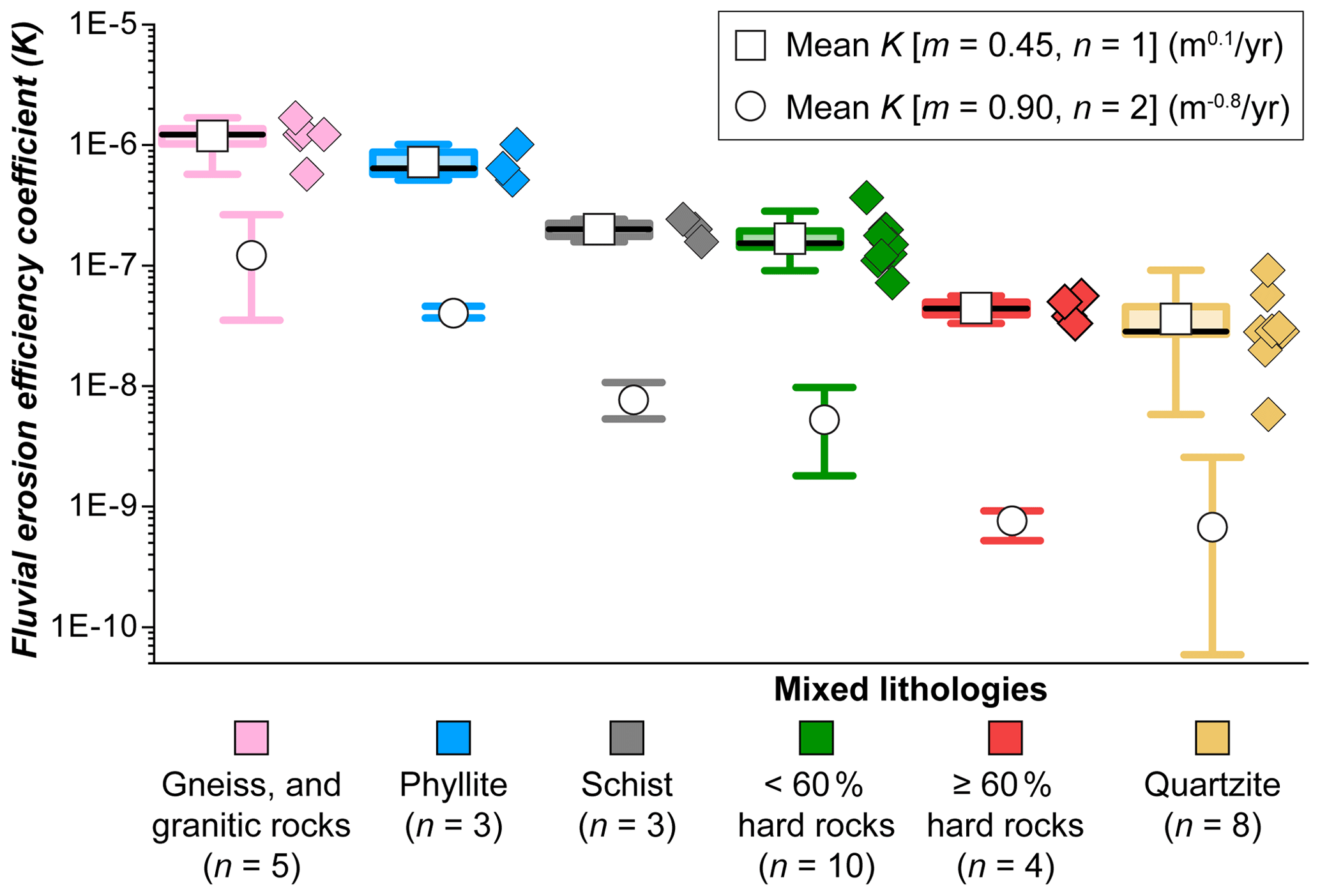
Figure 6Lithology controls the fluvial erosion efficiency coefficient (K) in the study area. Boxplot elements are as follows: box range represents the standard error of the mean, whisker range shows the interval between the 10th and 90th percentiles of the data, and the thick black line shows the median values. Note that we calculated K assuming (i) m=0.45 and n=1 (derived values of K have units of m0.1 yr−1) and (ii) m=0.9 and n=2 (derived values of K have units of m−0.8 yr−1). For the case of n=1, we show the boxplot on the left and raw data (diamonds) on the right. See Table S1 for data on each of the catchments analysed, including lithology and mean annual precipitation rates.
5.1 Equilibrium as a natural attractor state in a decaying mountain belt
Our results show that bedrock strength controls the variability in topographic relief and channel steepness in the QF. This conclusion is consistent with the classic geomorphic expectation that, all else being equal, terrains underlain by resistant rocks will develop higher topographic relief and steeper channel gradients (e.g. Gilbert, 1877; Hack, 1960; Jansen et al., 2010; Bursztyn et al., 2015). Such correlation between topographic forms and rock strength is the same as that expected in an equilibrium adjustment scenario for a tectonically stable erosive landscape evolving over timescales of millions of years (Hack, 1960; Montgomery, 2001). In the case of a spatially variable lithological configuration, theory predicts that more erodible rock units are progressively eroded, whereas resistant rocks stand proud in relief, up to a point where differential topographic steepness everywhere balances spatial variations in rock strength, and denudation rates are then spatially invariant (Hack, 1960). Our detrital cosmogenically-derived results, however, demonstrate that rates of denudation are kept spatially variable by the exposure at the surface of different rock types in a tectonically inactive landscape evolving for hundreds of millions of years. The landscape has not achieved any equilibrium or a steady state. We interpret our findings as an indication that equilibrium is likely not a natural attractor state in decaying mountain belts or is (at best) an attractor state that cannot be reached as long as lithological spatial heterogeneity (such as the one observed in the study area) is maintained, a conclusion that is consistent with the modelling results of Forte et al. (2016).
5.2 Lateral variations in rock type as a dominant control on denudation rates and topographic forms in a post-orogenic landscape
Our results suggest that the fluvial erosion efficiency coefficient (K) varies as a function of rock type in the study area, with low K values in resistant units and orders of magnitude higher K values in more erodible rocks. In contrast, we find that spatial gradients in precipitation rates do not control changes in K in the study area, considering that wetter climate conditions are generally associated with higher values of K (e.g. Ferrier et al., 2013). However, the fluvial erosion efficiency coefficient (K) as calculated here incorporates other effects besides rock strength and precipitation rates, such as channel hydraulic geometry and sediment load (e.g. Snyder et al., 2000; Duvall et al., 2004; Zondervan et al., 2020b). Whereas in the Appalachians effects on fluvial erosional efficiency such as channel width and sediment load have been shown to vary as a function of rock type (e.g. Spotila et al., 2015), we do not have data on such variables for the QF, which is a limitation to our reasonable interpretation that rock type controls K in the study area. We note, however, that rock strength varies within each rock type in the study area, and, for instance, thin-bedded quartzites with large quantities of muscovite and sericite weather and erode much more easily than average, while some granitic areas stand bold in relief where these rocks are coarser-grained and more massive (Dorr, 1969).
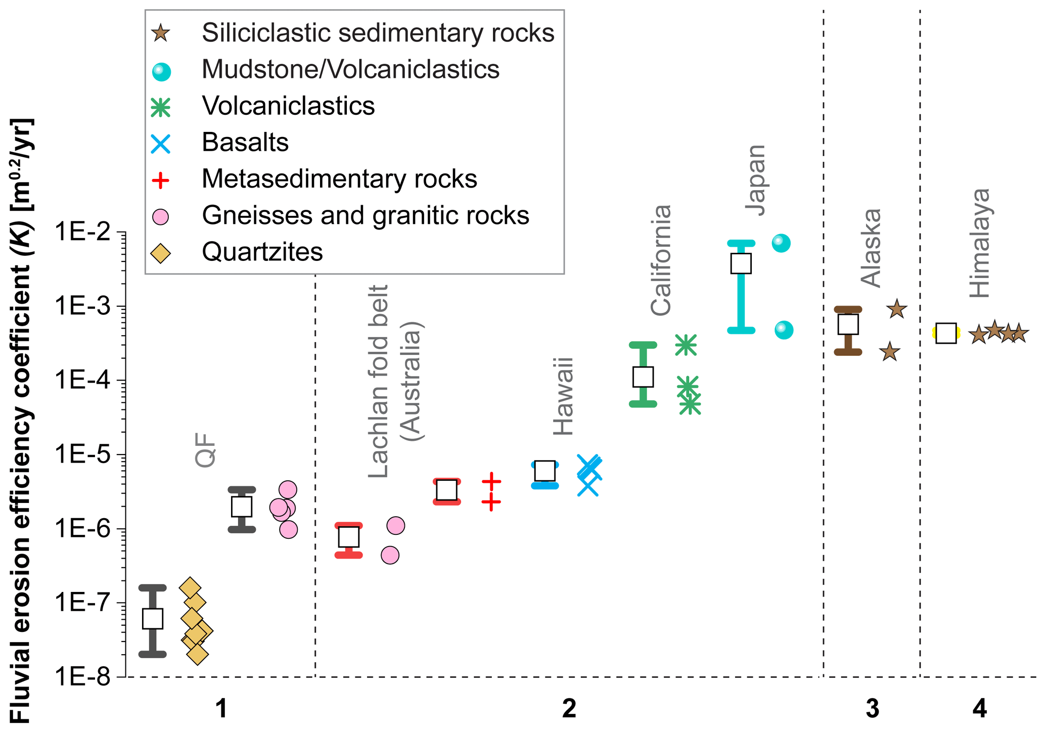
Figure 7Comparison of our results for the fluvial erosion efficiency coefficient (K) with previously published estimates of K. Note that we display whiskers (representing the interval between the 10th and 90th percentiles of the data) and mean values (white squares) on the left and raw data (diamonds) on the right. Estimates of K were derived assuming the slope exponent n=1. Numbers on the x axis represent different data sources: (1) this study; (2) Stock and Montgomery (1999); (3) Whipple et al. (2000b); (4) Kirby and Whipple (2001). Lithology was compiled as described by the respective authors of the above studies.
The negative relationships we find between 10Be-derived catchment-averaged denudation rates and catchment-averaged values of topographic relief, channel steepness and precipitation rates are counter-intuitive. However, such relationships are consistent with the stream power model if one accounts for the magnitude of variations in the fluvial erosion efficiency coefficient (K) estimated for the study area. Our findings agree with studies that demonstrate that the link between denudation rates and channel steepness is obscure in settings where lateral variations in rock strength are important (e.g. Cyr et al., 2014; Campforts et al., 2020) and that a modified version of the stream power model that includes variations in rock strength should be adopted for better predicting spatial patterns of channel incision (Campforts et al., 2020). Our results imply that modelling studies attempting to reconstruct uplift histories from river profile morphology assuming uniform fluvial erosion efficiency over large areas (e.g. Roberts and White, 2010) are likely to be flawed (at least in post-orogenic settings).
To compare our constraints on the fluvial erosion efficiency coefficient with published estimates of K, we also calculate K in units of m0.2 yr−1, as reported in several studies (e.g. Stock and Montgomery, 1999; Whipple et al., 2000b; Kirby and Whipple, 2001). We find that the resulting estimates of K in the QF (regional mean K value of m0.2 yr−1, assuming the slope exponent n=1) are comparable to or lower than the low end of the K values reported by Stock and Montgomery (1999) for a post-orogenic landscape underlain by granites and metasedimentary rocks in humid subtropical Australia (Fig. 7). Similarly, our estimates of K (in Fig. 6) are comparable to or lower than the low end of the K values estimated in crystalline and metamorphic rocks in the upper Tennessee River (mean K values of m0.1 yr−1; Gallen, 2018), as well as in different physiographic provinces in the Appalachians such as the Blue Ridge (reported K values: 7.8– m0.1 yr−1; Gallen et al., 2013) and the Valley and Ridge (reported K values: 2.1– m0.1 yr−1; Miller et al., 2013). In contrast, our results are orders of magnitude lower than estimates of K in tectonically active areas in Hawaii (tropical rainforest climate), California (Mediterranean climate), and Japan (humid continental climate; Stock and Montgomery, 1999), as well as the Siwalik Hills in the Himalayas (monsoon highland climate; Kirby and Whipple, 2001) and the Ukak River in Alaska (cool continental climate; Whipple et al., 2000b).
It is difficult to isolate the influence of rock strength from climate conditions in this comparison. Nonetheless, Fig. 7 suggests a stark contrast over orders of magnitude in the fluvial erosion efficiency coefficient between tectonically active and inactive settings, which may result from the disparity between the high rates of denudation in orogenic belts, with exposure of mineral surfaces that are readily weathered, and the long timescales of evolution in ancient mountain belts, where the hard metamorphic roots of these landscapes are progressively exhumed as these landscapes age (Summerfield and Hulton, 1994; Bishop, 2007; Braun et al., 2014; Bursztyn et al., 2015). In contrast, the global dataset of stream power model parameters reported by Harel et al. (2016) exhibits lower K values in tectonically active areas compared to higher K values in inactive settings. These authors concluded that such results were counter-intuitive and highlighted the fact that K is not well calibrated (Harel et al., 2016); more work needs to be dedicated to the determination of K and what controls its variations.
5.3 Landscape development in a decaying mountain belt marked by lateral contrasts in rock strength
Our findings indicate that high-relief uplands underlain by resistant bedrock are denuding more slowly than lower-relief surrounding areas associated with more erodible lithologies, with the corollary that topographic relief must still be growing instead of decaying in this tectonically quiescent landscape. Furthermore, the expected isostatic compensation to denudational unloading (e.g. Bishop and Brown, 1992), which is a process that occurs at a much longer wavelength than the local changes in lithology and denudation rates (Gilchrist and Summerfield, 1990; Watts et al., 2000), implies that uplands and surrounding areas are equally isostatically uplifted in response to the regional denudation, likely resulting in a net reduction of mean elevation over time but a slight increase in the heights of mountain peaks, as has been proposed by Molnar and England (1990). The timescale over which relief might continue to grow simply as a result of spatial variations in bedrock lithology is unresolved. However, our results suggest that relief is likely to persist long into the future in a landscape that would otherwise be suited to rapid denudation (high-relief and relatively high precipitation rates and warm climate).
Extrapolation of the denudation pattern in the QF over time, which is speculative for timescales more extended than the averaging of our cosmogenic data (Table S1), suggests that exposure at the surface of rocks with significant contrasts in erodibility naturally favours the survival of relief in the absence of ongoing tectonics. Nevertheless, we have compelling geomorphic evidence that at least some decaying mountain belts underwent spatial and temporal changes in denudation rates as a response to different types of forcing (e.g. tectonic, lithologic, climatic, mantle-driven, and far-field-driven) long after cessation of crustal thickening (e.g. Pazzaglia and Brandon, 1996; Quigley et al., 2007; Gallen et al., 2013; Tucker and van der Beek, 2013; Liu, 2014; Gallen, 2018). In this situation, large spatial contrasts in the fluvial erosion efficiency coefficient (K), such as observed in our study area, determine significant differences in erosional response times across the landscape (i.e. the timescale of channel profile response to perturbations in boundary conditions), with response times (Td) decreasing as K increases (Td scales to , where n is the slope exponent in the stream power model; Baldwin et al., 2013). Spatial gradients in K thus control how post-orogenic landscapes respond to a given force. Indeed, lithological controls on post-orogenic landscape dynamics have long been identified (e.g. Hack, 1960, 1975; Twidale, 1976; Mills, 2003; Bishop and Goldrick, 2010; Spotila et al., 2015; Gallen, 2018; Bernard et al., 2019; Vasconcelos et al., 2019; Zondervan et al., 2020a). Nonetheless, lithological contrasts have not been addressed adequately by numerical modelling of post-orogenic landscape evolution and, in particular, topographic decay (e.g. Baldwin et al., 2003; Egholm et al., 2013).
We present 10Be concentrations in river sand from catchments spanning the range of topographic metrics and bedrock erodibility in a humid subtropical, tectonically inactive landscape in Brazil. The results of this study suggest that the post-orogenic history of the study area is not a progressive reduction in relief and denudation rates. Instead, the exposure at the surface of rocks with strong lateral contrasts in erodibility amplifies spatial differences in topographic forms and denudation rates over time, sustaining or indeed increasing relief in a tectonically dead landscape. Spatial variations in topographic relief and channel steepness are explained by changes in rock type in the study area, and yet denudation rates are not spatially uniform. Contrasts in rock type continue to drive differences in denudation rates in a decaying mountain belt evolving over a timescale of millions of years, indicating that the landscape has not achieved equilibrium. This study demonstrates that lateral variations in rock strength play an essential role in the dynamics of an ancient mountain belt, and likely in other post-orogenic settings characterised by spatial heterogeneity in lithology. Such lithological heterogeneity controls the tempo and style of landscape response to changes in boundary conditions while also affecting the pattern of landscape denudation.
The data supporting the findings of this study are available in the Supplement, including 10Be analytical results and derived denudation rate data, catchment-averaged geomorphic parameters, and detailed information on catchment lithology. Extraction of topographic metrics and catchment-averaged pressure were carried out using LSDTopoTools version 2.03 (https://doi.org/10.5281/zenodo.3769703, Mudd et al., 2020).
The supplement related to this article is available online at: https://doi.org/10.5194/esurf-9-167-2021-supplement.
DP designed the study with contributions from all co-authors. DP and DF performed the cosmogenic isotope analysis. DP quantified the geomorphic parameters. DP, CP, MDH, PB and DF wrote the manuscript. DP produced the figures.
The authors declare that they have no conflict of interest.
We thank the German Aerospace Center (DLR), the Natural Environment Research Council (NERC), and the Coordination for the Improvement of Higher Education Personnel (CAPES) for research support. We thank Hugh D. Sinclair for providing feedback on an early version of the manuscript.
The DLR granted us access to TanDEM-X data as part of the project DEM_GEOL1345. NERC supported the cosmogenic isotope analysis under CIAF award no. 9177.0417. Daniel Peifer had support from CAPES under a Science without Borders fellowship (grant no. BEX 12000/13-2) and subsequently a CAPES-PrInt Postdoctoral fellowship (grant no. 88887.367976/2019-00).
This paper was edited by Greg Hancock and reviewed by one anonymous referee.
Ahnert, F.: Functional relationships between denudation, relief, and uplift in large, mid-latitude drainage basins, Am. J. Sci., 268, 243–263, https://doi.org/10.2475/ajs.268.3.243, 1970.
Alkmim, F. F. and Marshak, S.: Transamazonian orogeny in the Southern Sao Francisco craton region, Minas Gerais, Brazil: evidence for Paleoproterozoic collision and collapse in the Quadrilátero Ferrífero, Precambrian Res., 90, 29–58, https://doi.org/10.1016/S0301-9268(98)00032-1, 1998.
Alvares, C. A., Stape, J. L., Sentelhas, P. C., de Moraes Gonçalves, J. L., and Sparovek, G.: Köppen's climate classification map for Brazil, Meteorol. Z., 22, 711–728, https://doi.org/10.1127/0941-2948/2013/0507, 2013.
Balco, G., Stone, J. O., Lifton, N. A., and Dunai, T. J.: A complete and easily accessible means of calculating surface exposure ages or erosion rates from 10Be and 26Al measurements, Quat. Geochronol., 3, 174–195, https://doi.org/10.1016/j.quageo.2007.12.001, 2008.
Baldwin, J. A., Whipple, K. X., and Tucker, G. E.: Implications of the shear stress river incision model for the timescale of postorogenic decay of topography, J. Geophys. Res.-Solid, 108, 1–17, https://doi.org/10.1029/2001JB000550, 2003.
Barreto, H. N., Varajão, C. A., Braucher, R., Bourlès, D. L., Salgado, A. A., and Varajão, A. F.: Denudation rates of the Southern Espinhaço Range, Minas Gerais, Brazil, determined by in situ-produced cosmogenic beryllium-10, Geomorphology, 191, 1–13, https://doi.org/10.1016/j.geomorph.2013.01.021, 2013.
Beeson, H. W., McCoy, S. W., and Keen-Zebert, A.: Geometric disequilibrium of river basins produces long-lived transient landscapes, Earth Planet. Sc. Lett., 475, 34–43, https://doi.org/10.1016/j.epsl.2017.07.010, 2017.
Bernard, T., Sinclair, H. D., Gailleton, B., Mudd, S. M., and Ford, M.: Lithological control on the post-orogenic topography and erosion history of the Pyrenees, Earth Planet. Sc. Lett., 518, 53–66, https://doi.org/10.1016/j.epsl.2019.04.034, 2019.
Bierman, P. R. and Caffee, M.: Slow rates of rock surface erosion and sediment production across the Namib Desert and escarpment, southern Africa, Am. J. Sci., 301, 326–358, https://doi.org/10.2475/ajs.301.4-5.326, 2001.
Bishop, P.: Long-term landscape evolution: linking tectonics and surface processes, Earth Surf. Proc. Land., 32, 329–365, https://doi.org/10.1002/esp.1493, 2007.
Bishop, P. and Brown, R.: Denudational isostatic rebound of intraplate highlands: the Lachlan River valley, Australia, Earth Surf. Proc. Land., 17, 345–360, https://doi.org/10.1002/esp.3290170405, 1992.
Bishop, P. and Goldrick, G.: Lithology and the evolution of bedrock rivers in post-orogenic settings: constraints from the high-elevation passive continental margin of SE Australia, Geol. Soc. Spec. Publ., 346, 267–287, https://doi.org/10.1144/SP346.14, 2010.
Blackburn, T., Ferrier, K. L., and Perron, J. T.: Coupled feedbacks between mountain erosion rate, elevation, crustal temperature, and density, Earth Planet. Sc. Lett., 498, 377–386, https://doi.org/10.1016/j.epsl.2018.07.003, 2018.
Braun, J., Simon-Labric, T., Murray, K. E., and Reiners, P. W.: Topographic relief driven by variations in surface rock density, Nat. Geosci., 7, 534–540, https://doi.org/10.1038/NGEO2171, 2014.
Bursztyn, N., Pederson, J. L., Tressler, C., Mackley, R. D., and Mitchell, K. J.: Rock strength along a fluvial transect of the Colorado Plateau–quantifying a fundamental control on geomorphology, Earth Planet. Sc. Lett., 429, 90–100, https://doi.org/10.1016/j.epsl.2015.07.042, 2015.
Campforts, B., Vanacker, V., Herman, F., Vanmaercke, M., Schwanghart, W., Tenorio, G. E., Willems, P., and Govers, G.: Parameterization of river incision models requires accounting for environmental heterogeneity: insights from the tropical Andes, Earth Surf. Dynam., 8, 447–470, https://doi.org/10.5194/esurf-8-447-2020, 2020.
Chemale Jr., F., Rosière, C. A., and Endo, I.: The tectonic evolution of the Quadrilátero Ferrífero, Minas Gerais, Brazil, Precambrian Res., 65, 25–54, https://doi.org/10.1016/0301-9268(94)90098-1, 1994.
Clubb, F. J., Bookhagen, B., and Rheinwalt, A.: Clustering river profiles to classify geomorphic domains, J. Geophys. Res.-Earth, 124, 1417–1439, https://doi.org/10.1029/2019JF005025, 2019.
Cyr, A. J., Granger, D. E., Olivetti, V., and Molin, P.: Distinguishing between tectonic and lithologic controls on bedrock channel longitudinal profiles using cosmogenic 10Be erosion rates and channel steepness index, Geomorphology, 209, 27–38, https://doi.org/10.1016/j.geomorph.2013.12.010, 2014.
Davis, W. M.: The geographical cycle, Geogr. J., 14, 481–504, https://doi.org/10.2307/1774538, 1899.
DiBiase, R. A.: Increasing vertical attenuation length of cosmogenic nuclide production on steep slopes negates topographic shielding corrections for catchment erosion rates, Earth Surf. Dynam., 6, 923–931, https://doi.org/10.5194/esurf-6-923-2018, 2018.
DiBiase, R. A. and Whipple, K. X.: The influence of erosion thresholds and runoff variability on the relationships among topography, climate, and erosion rate, J. Geophys. Res.-Earth, 116, 1–17, https://doi.org/10.1029/2011JF002095, 2011.
DiBiase, R. A., Whipple, K. X., Heimsath, A. M., and Ouimet, W. B.: Landscape form and millennial erosion rates in the San Gabriel Mountains, CA, Earth Planet. Sc. Lett., 289, 134–144, https://doi.org/10.1016/j.epsl.2009.10.036, 2010.
Dorr, J. V. N.: Physiographic, stratigraphic, and structural development of the Quadrilátero Ferrífero, Minas Gerais, Brazil, United States Geological Survey Professional Paper 641-A, US Geological Survey, Washington, D.C., 1969.
Duvall, A., Kirby, E., and Burbank, D.: Tectonic and lithologic controls on bedrock channel profiles and processes in coastal California, J. Geophys. Res.-Earth, 109, 1–18, https://doi.org/10.1029/2003JF000086, 2004.
Egholm, D. L., Knudsen, M. F., and Sandiford, M.: Lifespan of mountain ranges scaled by feedbacks between landsliding and erosion by rivers, Nature, 498, 475–478, https://doi.org/10.1038/nature12218, 2013.
Ferrier, K. L., Huppert, K. L., and Perron, J. T.: Climatic control of bedrock river incision, Nature, 496, 206–209, https://doi.org/10.1038/nature11982, 2013.
Fick, S. E. and Hijmans, R. J.: WorldClim 2: new 1-km spatial resolution climate surfaces for global land areas, Int. J. Climatol., 37, 4302–4315, https://doi.org/10.1002/joc.5086, 2017.
Flint, J. J.: Stream gradient as a function of order, magnitude, and discharge, Water Resour. Res., 10, 969–973, https://doi.org/10.1029/WR010i005p00969, 1974.
Forte, A. M., Yanites, B. J., and Whipple, K. X.: Complexities of landscape evolution during incision through layered stratigraphy with contrasts in rock strength, Earth Surf. Proc. Land., 41, 1736–1757, https://doi.org/10.1002/esp.3947, 2016.
Gallen, S. F.: Lithologic controls on landscape dynamics and aquatic species evolution in post-orogenic mountains, Earth Planet. Sc. Lett., 493, 150–160, https://doi.org/10.1016/j.epsl.2018.04.029, 2018.
Gallen, S. F., Wegmann, K. W., and Bohnenstiehl, D. R.: Miocene rejuvenation of topographic relief in the southern Appalachians, GSA Today, 23, 4–10, https://doi.org/10.1130/GSATG163A.1, 2013.
Gilbert, G.: Geology of the Henry Mountains, USGS Unnumbered Series, Government Printing Office, Washington, D.C., USA, https://doi.org/10.3133/70038096, 1877.
Gilchrist, A. R. and Summerfield, M. A.: Differential denudation and flexural isostasy in formation of rifted-margin upwarps, Nature, 346, 739–742, https://doi.org/10.1038/346739a0, 1990.
Hack, J. T.: Interpretation of erosional topography in humid temperate regions, Am. J. Sci., 258, 80–97, 1960.
Hack, J. T.: Dynamic equilibrium and landscape evolution, in: Theories of landform development, edited by: Melhorn, W. N. and Flemal, R. C., State University of New York Press, Binghamton, NY, USA, 87–102, 1975.
Hack, J. T.: Physiographic divisions and differential uplift in the Piedmont and Blue Ridge, United States Geological Survey Professional Paper 1265, US Geological Survey, Washington, D.C., 1982.
Harel, M. A., Mudd, S. M., and Attal, M.: Global analysis of the stream power law parameters based on worldwide 10Be denudation rates, Geomorphology, 268, 184–196, https://doi.org/10.1016/j.geomorph.2016.05.035, 2016.
Hergarten, S., Robl, J., and Stüwe, K.: Tectonic geomorphology at small catchment sizes-extensions of the stream-power approach and the χ method, Earth Surf. Dynam., 4, 1–9, https://doi.org/10.5194/esurf-4-1-2016, 2016.
Howard, A. D. and Kerby, G.: Channel changes in badlands, GSA Bull., 94, 739–752, https://doi.org/10.1130/0016-7606(1983)94<739:CCIB>2.0.CO;2, 1983.
Hurst, M. D., Ellis, M. A., Royse, K. R., Lee, K. A., and Freeborough, K.: Controls on the magnitude-frequency scaling of an inventory of secular landslides, Earth Surf. Dynam., 1, 67–78, https://doi.org/10.5194/esurf-1-67-2013, 2013.
Jansen, J. D., Codilean, A. T., Bishop, P., and Hoey, T. B.: Scale dependence of lithological control on topography: Bedrock channel geometry and catchment morphometry in western Scotland, J. Geol., 118, 223–246, https://doi.org/10.1086/651273, 2010.
Kirby, E. and Whipple, K. X.: Quantifying differential rock-uplift rates via stream profile analysis, Geology, 29, 415–418, https://doi.org/10.1130/0091-7613(2001)029<0415:QDRURV>2.0.CO;2, 2001.
Kirby, E. and Whipple, K. X.: Expression of active tectonics in erosional landscapes, J. Struct. Geol., 44, 54–75, https://doi.org/10.1016/j.jsg.2012.07.009, 2012.
Kohl, C. P. and Nishiizumi, K.: Chemical isolation of quartz for measurement of in-situ-produced cosmogenic nuclides, Geochim. Cosmochim. Ac., 56, 3583–3587, https://doi.org/10.1016/0016-7037(92)90401-4, 1992.
Korup, O.: Rock type leaves topographic signature in landslide-dominated mountain ranges, Geophys. Res. Lett., 35, 1–5, https://doi.org/10.1029/2008GL034157, 2008.
Lague, D.: The stream power river incision model: evidence, theory and beyond, Earth Surf. Proc. Land., 39, 38–61, https://doi.org/10.1002/esp.3462, 2014.
Lague, D., Davy, P., and Crave, A.: Estimating uplift rate and erodibility from the area-slope relationship: Examples from Brittany (France) and numerical modelling, Phys. Chem. Earth Pt. A, 25, 543–548, https://doi.org/10.1016/S1464-1895(00)00083-1, 2000.
Lal, D.: Cosmic ray labeling of erosion surfaces: in situ nuclide production, Earth Planet. Sc. Lett., 104, 424–439, https://doi.org/10.1016/0012-821X(91)90220-C, 1991.
Liu, L.: Rejuvenation of Appalachian topography caused by subsidence-induced differential erosion, Nat. Geosci., 7, 518–523, https://doi.org/10.1038/NGEO2187, 2014.
Lobato, L., Ribeiro-Rodrigues, L., Zucchetti, M., Noce, C., Baltazar, O., Da Silva, L., and Pinto, C.: Brazil's premier gold province. Part I: The tectonic, magmatic, and structural setting of the Archean Rio das Velhas greenstone belt, Quadrilátero Ferrífero, Miner. Deposita., 36, 228–248, https://doi.org/10.1007/s001260100179, 2001.
Lobato, L. M., Baltazar, O. F., Reis, L. B., Achtschin, A. B., Baars, F. J., Timbó, M. A., Berni, G. V., de Mendonça, B. R. V., and Ferreira, D. V: Projeto Geologia do Quadrilátero Ferrífero – Integração e Correção Cartográfica em SIG com Nota Explicativa, CODEMIG, Belo Horizonte, 2005.
Mandal, S. K., Lupker, M., Burg, J. P., Valla, P. G., Haghipour, N., and Christl, M.: Spatial variability of 10Be-derived erosion rates across the southern Peninsular Indian escarpment: A key to landscape evolution across passive margins, Earth Planet. Sc. Lett., 425, 154–167, https://doi.org/10.1016/j.epsl.2015.05.050, 2015.
Matmon, A., Bierman, P. R., Larsen, J., Southworth, S., Pavich, M., and Caffee, M.: Temporally and spatially uniform rates of erosion in the southern Appalachian Great Smoky Mountains, Geology, 31, 155–158, https://doi.org/10.1130/0091-7613(2003)031<0155:TASURO>2.0.CO;2, 2003.
Meybeck, M.: Global chemical weathering of surficial rocks estimated from river dissolved loads, Am. J. Sci., 287, 401–428, https://doi.org/10.2475/ajs.287.5.401, 1987.
Miller, S. R., Sak, P. B., Kirby, E., and Bierman, P. R.: Neogene rejuvenation of central Appalachian topography: Evidence for differential rock uplift from stream profiles and erosion rates, Earth Planet. Sc. Lett., 369, 1–12, https://doi.org/10.1016/j.epsl.2013.04.007, 2013.
Mills, H. H.: Inferring erosional resistance of bedrock units in the east Tennessee mountains from digital elevation data, Geomorphology, 55, 263–281, https://doi.org/10.1016/S0169-555X(03)00144-2, 2003.
Molnar, P. and England, P.: Late Cenozoic uplift of mountain ranges and global climate change: chicken or egg?, Nature, 346, 29–34, https://doi.org/10.1038/346029a0, 1990.
Monteiro, H. S., Vasconcelos, P. M., Farley, K. A., Spier, C. A., and Mello, C. L.: (U–Th)/He geochronology of goethite and the origin and evolution of cangas, Geochim. Cosmochim. Ac., 131, 267–289, https://doi.org/10.1016/j.gca.2014.01.036, 2014.
Monteiro, H. S., Vasconcelos, P. M., and Farley, K. A.: A combined (U-Th)/He and cosmogenic 3He record of landscape armoring by biogeochemical iron cycling, J. Geophys. Res.-Earth, 123, 298–323, https://doi.org/10.1002/2017JF004282, 2018.
Montgomery, D. R.: Slope distributions, threshold hillslopes, and steady-state topography, Am. J. Sci., 301, 432–454, https://doi.org/10.2475/ajs.301.4-5.432, 2001.
Montgomery, D. R. and Brandon, M. T.: Topographic controls on erosion rates in tectonically active mountain ranges, Earth Planet. Sc. Lett., 201, 481–489, https://doi.org/10.1016/S0012-821X(02)00725-2, 2002.
Moon, S., Chamberlain, C. P., Blisniuk, K., Levine, N., Rood, D. H., and Hilley, G. E.: Climatic control of denudation in the deglaciated landscape of the Washington Cascades, Nat. Geosci., 4, 469–473, https://doi.org/10.1038/NGEO1159, 2011.
Mudd, S. M., Attal, M., Milodowski, D. T., Grieve, S. W., and Valters, D. A.: A statistical framework to quantify spatial variation in channel gradients using the integral method of channel profile analysis, J. Geophys. Res.-Earth, 119, 138–152, https://doi.org/10.1002/2013JF002981, 2014.
Mudd, S. M., Harel, M. A., Hurst, M. D., Grieve, S. W., and Marrero, S. M.: The CAIRN method: automated, reproducible calculation of catchment-averaged denudation rates from cosmogenic nuclide concentrations, Earth Surf. Dynam., 4, 655–674, https://doi.org/10.5194/esurf-4-655-2016, 2016.
Mudd, S. M., Clubb, F. J., Gailleton, B., and Hurst, M. D.: How concave are river channels?, Earth Surf. Dynam., 6, 505–523, https://doi.org/10.5194/esurf-6-505-2018, 2018.
Mudd, S. M., Clubb, F. J., and Hurst, M. D.: LSDTopoTools2 v0.3, Zenodo, https://doi.org/10.5281/zenodo.3769703, 2020.
Myers, R. H.: Classical and modern regression with applications, 2nd Edn., Duxbury Press, Boston, MA, USA, 1990.
Pazzaglia, F. J. and Brandon, M. T.: Macrogeomorphic evolution of the post-Triassic Appalachian mountains determined by deconvolution of the offshore basin sedimentary record, Basin Res., 8, 255–278, https://doi.org/10.1046/j.1365-2117.1996.00274.x, 1996.
Perne, M., Covington, M. D., Thaler, E. A., and Myre, J. M.: Steady state, erosional continuity, and the topography of landscapes developed in layered rocks, Earth Surf. Dynam., 5, 85–100, https://doi.org/10.5194/esurf-5-85-2017, 2017.
Perron, J. T. and Royden, L.: An integral approach to bedrock river profile analysis, Earth Surf. Proc. Land., 38, 570–576, https://doi.org/10.1002/esp.3302, 2013.
Portenga, E. W. and Bierman, P. R.: Understanding Earth's eroding surface with 10Be, GSA Today, 21, 4–10, https://doi.org/10.1130/G111A.1, 2011.
Quigley, M., Sandiford, M., Fifield, K., and Alimanovic, A.: Bedrock erosion and relief production in the northern Flinders Ranges, Australia, Earth Surf. Proc. Land., 32, 929–944, https://doi.org/10.1002/esp.1459, 2007.
Roberts, G. G. and White, N.: Estimating uplift rate histories from river profiles using African examples, J. Geophys. Res.-Earth, 115, 1–24, https://doi.org/10.1029/2009JB006692, 2010.
Salgado, A. A. R., Braucher, R., Varajão, A. C., Colin, F., Varajão, A. F. D. C., and Nalini Jr., H. A.: Relief evolution of the Quadrilátero Ferrífero (Minas Gerais, Brazil) by means of (10Be) cosmogenic nuclei, Z. Geomorphol., 52, 317–323, https://doi.org/10.1127/0372-8854/2008/0052-0317, 2008.
Sant'Anna, L. G., Schorscher, H. D., and Riccomini, C.: Cenozoic tectonics of the Fonseca basin region, eastern Quadrilátero Ferrífero, MG, Brazil, J. S. Am. Earth Sci., 10, 275–284, https://doi.org/10.1016/S0895-9811(97)00016-3, 1997.
Scharf, T. E., Codilean, A. T., De Wit, M., Jansen, J. D., and Kubik, P. W.: Strong rocks sustain ancient postorogenic topography in southern Africa, Geology, 41, 331–334, https://doi.org/10.1130/G33806.1, 2013.
Snyder, N. P., Whipple, K. X., Tucker, G. E., and Merritts, D. J.: Landscape response to tectonic forcing: Digital elevation model analysis of stream profiles in the Mendocino triple junction region, northern California, GSA Bull., 112, 1250–1263, https://doi.org/10.1130/0016-7606(2000)112<1250:LRTTFD>2.0.CO;2, 2000.
Spier, C. A., Vasconcelos, P. M., and Oliviera, S. M.: geochronological constraints on the evolution of lateritic iron deposits in the Quadrilátero Ferrífero, Minas Gerais, Brazil, Chem. Geol., 234, 79–104, https://doi.org/10.1016/j.chemgeo.2006.04.006, 2006.
Spotila, J. A., Moskey, K. A., and Prince, P. S.: Geologic controls on bedrock channel width in large, slowly-eroding catchments: Case study of the New River in eastern North America, Geomorphology, 230, 51–63, https://doi.org/10.1016/j.geomorph.2014.11.004, 2015.
Stock, J. D. and Montgomery, D. R.: Geologic constraints on bedrock river incision using the stream power law, J. Geophys. Res.-Solid, 104, 4983–4993, https://doi.org/10.1029/98JB02139, 1999.
Stone, J. O.: Air pressure and cosmogenic isotope production, J. Geophys. Res.-Solid, 105, 23753–23759, https://doi.org/10.1029/2000JB900181, 2000.
Strahler, A. N.: Quantitative analysis of watershed geomorphology, Eos, 38, 913–920, https://doi.org/10.1029/TR038i006p00913, 1957.
Summerfield, M. A. and Hulton, N. J.: Natural controls of fluvial denudation rates in major world drainage basins, J. Geophys. Res.-Solid, 99, 13871–13883, https://doi.org/10.1029/94JB00715, 1994.
Tucker, G. E. and van Der Beek, P.: A model for post-orogenic development of a mountain range and its foreland, Basin Res., 25, 241–259, https://doi.org/10.1111/j.1365-2117.2012.00559.x, 2013.
Twidale, C. R.: On the survival of paleoforms, Am. J. Sci., 276, 77–95, https://doi.org/10.2475/ajs.276.1.77, 1976.
Vasconcelos, P. M. and Carmo, I. D. O.: Calibrating denudation chronology through weathering geochronology, Earth-Sci. Rev., 179, 411–435, https://doi.org/10.1016/j.earscirev.2018.01.003, 2018.
Vasconcelos, P. M., Farley, K. A., Stone, J., Piacentini, T., and Fifield, L. K.: Stranded landscapes in the humid tropics: Earth's oldest land surfaces, Earth Planet. Sc. Lett., 519, 152–164, https://doi.org/10.1016/j.epsl.2019.04.014, 2019.
von Blanckenburg, F., Hewawasam, T., and Kubik, P. W.: Cosmogenic nuclide evidence for low weathering and denudation in the wet, tropical highlands of Sri Lanka, J. Geophys. Res.-Earth, 109, 1–22, https://doi.org/10.1029/2003JF000049, 2004.
Watts, A. B., McKerrow, W. S., and Fielding, E.: Lithospheric flexure, uplift, and landscape evolution in south-central England, J. Geol. Soc., 157, 1169–1177, https://doi.org/10.1144/jgs.157.6.1169, 2000.
Whipple, K. X. and Tucker, G. E.: Dynamics of the stream-power river incision model: Implications for height limits of mountain ranges, landscape response timescales, and research needs, J. Geophys. Res.-Solid, 104, 17661–17674, https://doi.org/10.1029/1999JB900120, 1999.
Whipple, K. X., Hancock, G. S., and Anderson, R. S.: River incision into bedrock: Mechanics and relative efficacy of plucking, abrasion, and cavitation, GSA Bull., 112, 490–503, https://doi.org/10.1130/0016-7606(2000)112<490:RIIBMA>2.0.CO;2, 2000a.
Whipple, K. X., Snyder, N. P., and Dollenmayer, K.: Rates and processes of bedrock incision by the Upper Ukak River since the 1912 Novarupta ash flow in the Valley of Ten Thousand Smokes, Alaska, Geology, 28, 835–838, https://doi.org/10.1130/0091-7613(2000)28<835:RAPOBI>2.0.CO;2, 2000b.
White, A. F. and Blum, A. E.: Effects of climate on chemical weathering in watersheds, Geochim. Cosmochim. Ac., 59, 1729–1747, https://doi.org/10.1016/0016-7037(95)00078-E, 1995.
Zondervan, J. R., Stokes, M., Boulton, S. J., Telfer, M. W., and Mather, A. E.: Rock strength and structural controls on fluvial erodibility: Implications for drainage divide mobility in a collisional mountain belt, Earth Planet. Sc. Lett., 538, 1–13, https://doi.org/10.1016/j.epsl.2020.116221, 2020a.
Zondervan, J. R., Whittaker, A. C., Bell, R. E., Watkins, S. E., Brooke, S. A., and Hann, M. G.: New constraints on bedrock erodibility and landscape response times upstream of an active fault, Geomorphology, 351, 1–14, https://doi.org/10.1016/j.geomorph.2019.106937, 2020b.