Hack distributions of rill networks and nonlinear slope length–soil loss relationships

Surface flow on rilled hillslopes tends to produce sediment yields that scale nonlinearly with total hillslope length. The widespread observation lacks a single unifying theory for such a nonlinear relationship. We explore the contribution of rill network geometry to the observed yield–length scaling relationship. Relying on an idealized network geometry, we formally develop probability functions for geometric variables of contributing area and rill length. In doing so, we contribute towards a complete probabilistic foundation for the Hack distribution. Using deterministic and empirical functions, we then extend the probability theory to the hydraulic variables that are related to sediment detachment and transport. A Monte Carlo simulation samples hydraulic variables from hillslopes of different lengths to provide estimates of sediment yield. The results of this analysis demonstrate a nonlinear yield–length relationship as a result of the rill network geometry. Theory is supported by numerical modeling, wherein surface flow is routed over an idealized numerical surface and a natural surface from northern Arizona. Numerical flow routing demonstrates probability functions that resemble the theoretical ones. This work provides a unique application of the Scheidegger network to hillslope settings which, because of their finite lengths, result in unique probability functions. We have addressed sediment yields on rilled slopes and have contributed towards understanding Hack's law from a probabilistic reasoning.

1 Introduction

Rilled hillslopes are common in semiarid, agricultural, and recently disturbed landscapes (Fig. 1). In these settings, rills concentrate surface flow and serve as pathways for sediment transport and erosion. There is a long legacy of work that explores the mechanics and consequences of rill processes through field observation, experimentation (Govers, 1992; Liu et al., 2000), and numerical simulation (Hairsine and Rose, 1992; McGuire et al., 2013). This body of work highlights a number of key observations and relationships. Among these is the observation that sediment yield at the base of a hillslope tends to vary nonlinearly with the total length of the hillslope, L_h (L), so that $Q_{\mathrm{s}}\propto L_{\mathrm{h}}^{\mathit{\beta }}$, where Q_s (L³ T⁻¹) is the volumetric sediment yield and $\mathrm{1.4}\le \mathit{\beta }\le \mathrm{2.0}$ (McCool et al., 1993; Govers et al., 2007; Renard, 1997). Here, we consider the role of the rill network geometry in contributing to this nonlinear relationship.

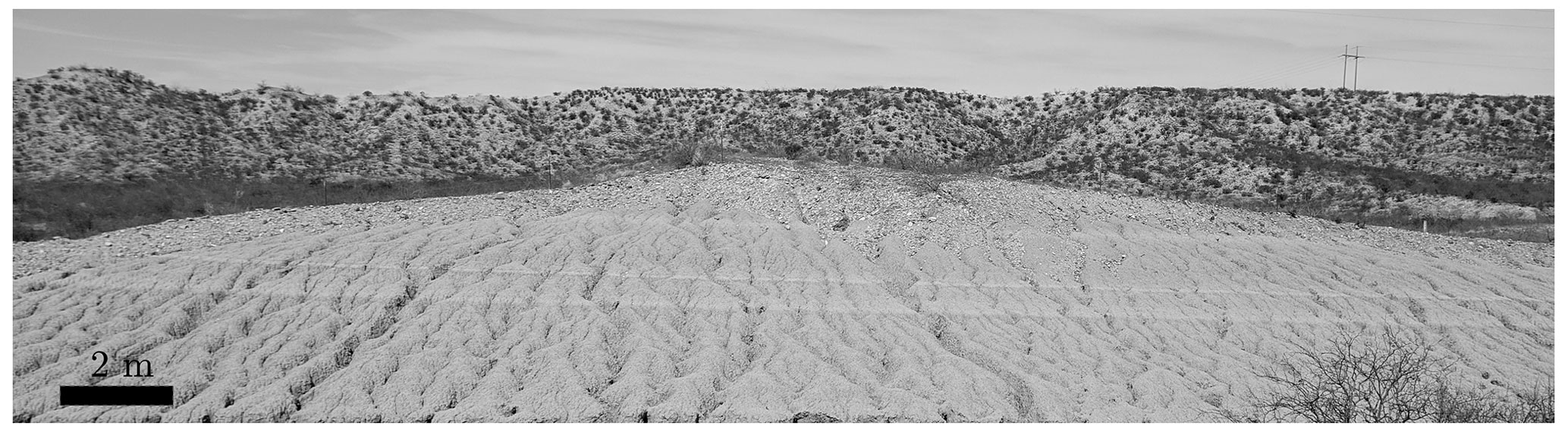
Figure 1 A rilled hillslope near Benson, AZ. Prominent sub-horizontal lines are the stratigraphy of the lake sediments of the region.

Nonlinear scaling relationships between sediment yield and slope length have been observed on all slopes for which surface flow is a dominant sediment transport mechanism. Moore and Burch (1986) consider surface flow over smooth hillslopes. By rearranging Manning's equation and solving for unit stream power, those authors demonstrate that a planar hillslope will generate a nonlinear relationship between sediment yield and slope length that is $Q_{\mathrm{s}}\propto L_{\mathrm{h}}^{\mathrm{1.4}}$. Note that this nonlinear relationship is the lower end of those identified for rilled hillslopes. Nonlinear relationships with an exponent greater than 1.4 require that flow concentrates as it moves downslope (Moore and Burch, 1986). Rill networks may form a range of geometries from nearly parallel paths that rarely converge to dendritic networks. These different rill network geometries may contribute towards a range of nonlinear yield–slope length relationships.

The causes of linear and dendritic networks is extensively explored by McGuire et al. (2013). In a numerical exploration, those authors demonstrate that the geometry of rill networks reflects the relative magnitudes of transport due to surface flow and rain splash. In this framework, surface flow tends to create straighter rills that converge less frequently. In contrast, transport due to rain splash is diffusive and tends to disrupt the linear channels, which leads to increasingly dendritic networks. In this paper, we consider the contributions from the geometry of dendritic networks which concentrate flow.

We develop a probability theory for the geometric variables of watershed length, l (L), and contributing area, A (L²), for an idealized rill network. From this theoretical starting point, we then extend the analysis to hydraulic variables that are related to sediment detachment and transport. This work is related to a suite of previous studies that incorporate probabilistic approaches to rill transport and dynamics. Most notably, our approach is similar to two previous studies. First, Lewis et al. (1994a, b) develop a stochastic model (PRORIL) for rill development and sediment transport that includes variable drainage density and flow rate. In this work, the authors present the model as a tool to explore the development of rill networks. Second, Damron and Winter (2008) employ a dynamic but idealized rill network wherein links between nodes can change based on a node's history. They use this model to demonstrate the temporal characteristics of sediment passing by a node as a result of the dynamics that occur in upslope links. These contributions effectively demonstrate the details and dynamics of rilled settings, but a description of the underlying probability functions of the networks and how they relate to slope length–sediment yield relationships remains outstanding.

Other probabilistic approaches have been applied to rill settings. Nearing (1991) considered the probability of particle entrainment as a result of the overlapping distributions of instantaneous shear stress and soil resistance. They demonstrate that this leads to the ability for flows to entrain sediment from soils that are relatively strong. Similarly, Mei et al. (2008) consider the rill width as a random variable, which influences flow depth and shear stress. Using a linearized perturbation method, they demonstrate the impact on statistical moments of hydraulic variables of flow velocity and depth. Our work considers the probability involved with the macroscale patterns of rill networks and, in principle, could be combined with these efforts that describe dynamics within rills.

We have two goals. First is to provide a rigorous probabilistic description of the rill network. In particular, we wish to formally develop the conditional distribution, f_A(A|l), which is read as the probability distribution of contributing area, A, given that a watershed has a length l, which is also a random variable with distribution f_l(l). These two distributions combine to create the joint distribution $f_{A,l}(A,l)$. This is the Hack distribution, which has been extensively studied and used to identify patterns in landscapes, but to date a complete derivation of the distributions remains to be done (Hack, 1957; Gupta et al., 1996; Dodds and Rothman, 2000). Second, we ask if a well-defined network of rills focuses flow such that it leads to a nonlinear sediment yield relationship with hillslope length, $Q_{\mathrm{s}}\propto L_{\mathrm{h}}^{\mathit{\beta }}$. Addressing these goals involves two approaches. First we extend the probability theory for topographic variables to hydraulic and sediment transport variables of unit stream power, shear stress, and sediment concentration. Second, we numerically route flow down the idealized and natural rill networks to evaluate and inform the theory.

The work presented in this paper builds largely on the results presented by Dodds and Rothman (2000). Those authors use the Scheidegger model, Hack's law, and some reasonable assumptions to inform a development of the form of probability functions for geometric variables. Starting with Hack's law, which relates the expected length of a watershed to its area, the authors assume that the conditional distribution, f_l(l|A), is Gaussian in form. From this assumption and known properties of random walks, they are able to develop functional forms for all distributions related to the joint distribution $f_{A,l}(A,l)$ (i.e., they develop the joint distribution, both forms of conditional distributions, and the marginal distributions). However, because their work involved an assumption of the form, the parameters of the distribution lack a formal development. In this paper, we lean heavily on this work but contribute towards a more formal understanding of the parameters of the distributions.

Before moving on, here is a note about notation. We use f_x(x;y) to denote a probability density or probability mass function for the random variable x with parameter y. The subscript indicates the random variable for the probability function. This becomes useful later.

2 Theory

2.1 Network geometry

We develop a theory for rill network geometry that is based on the Scheidegger model (Scheidegger, 1967). These networks have two characteristics. First, for every unit distance downslope, a rill has equal probability of moving half a unit left or right. Second, uniform drainage density is maintained, such that where two rills converge, which leaves one downslope node empty, a new rill is generated at the empty node (Fig. 2a). These two rules sufficiently describe the network and allow for us to develop theoretical distributions concerning the rill lengths, contributing areas, and flow variables for simple conditions. Other network classes exist including optimal channel networks (OCNs) and Peano basins (Maritan et al., 2002; Yi et al., 2018). Optimal channel networks are constructed by iterative numerical procedures that minimize the energy expenditure within the network (Rinaldo et al., 1993). As such, there are a great number of network configurations that satisfy the constraint, and there are not clear rules for the construction of links and rill paths. Peano networks are a class of self-similar trees wherein perpendicular tributaries are recursively added to the network at finer scales (Gupta et al., 1996). On hillslopes flow is in one dominant direction, and thus this model is unrealistic.

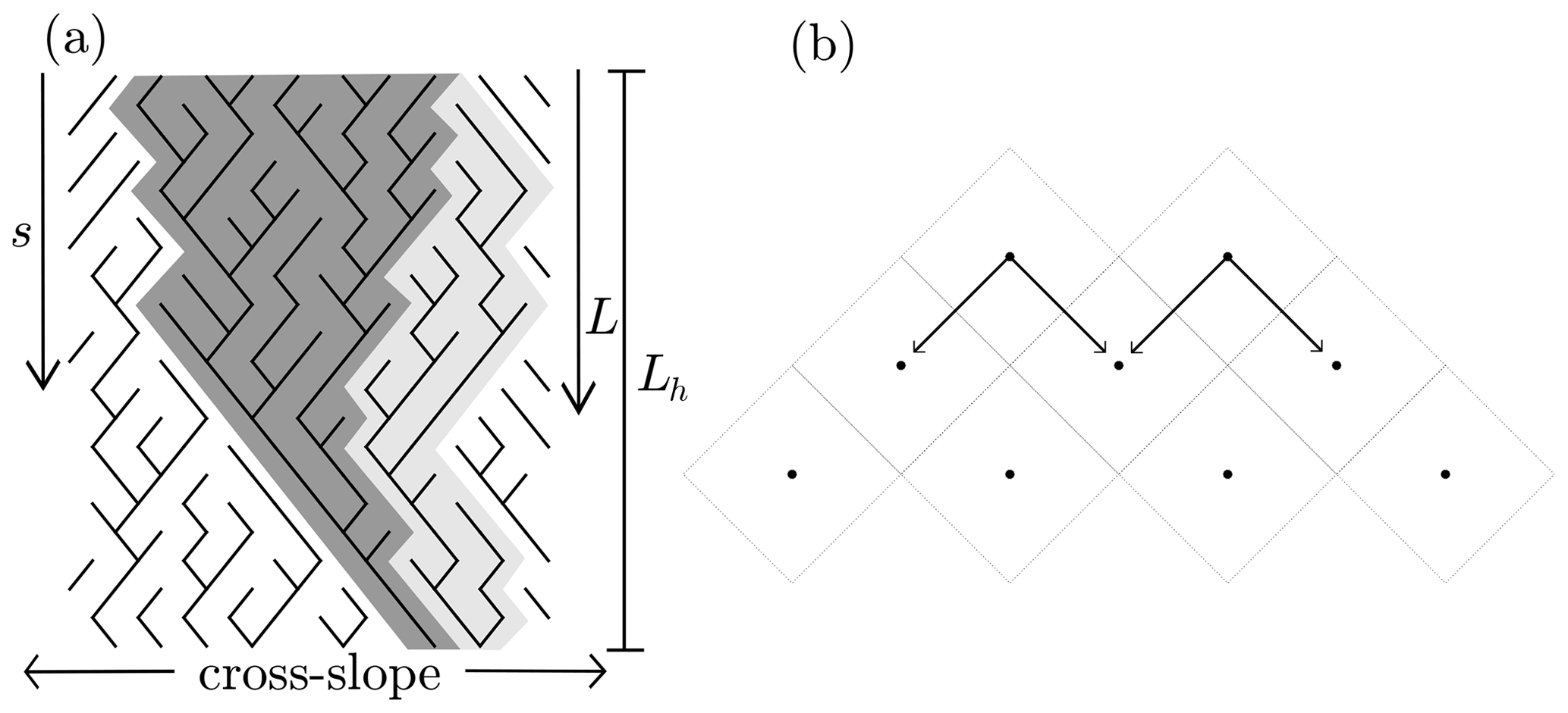
Figure 2 (a) Paths of one realization of a Scheidegger network with open (dark gray) and closed (light gray) watersheds highlighted. (b) Illustration of the grid and possible paths of links. Nodes are offset at downslope levels. A square grid is shown here, but there is no requirement that it be square.

2.2 Hack's law

Central to this work is Hack's Law, which is a nearly universal empirical scaling observation where the length of the main channel is related to the contributing area by an exponent,

$$\begin{array}{}\text{(1)}& l=\mathit{\theta }{A}^m,\end{array}$$

where l is the length of the main channel, A is the contributing area, and θ is a dimensional coefficient. The exponent m is the subject of work that explores the fractal characteristics of networks (Hack, 1957; Dodds and Rothman, 2000; Maritan et al., 2002; Bennett and Liu, 2016). We choose to rewrite Hack's law with l as the independent variable,

$$\begin{array}{}\text{(2)}& A=\mathit{\varphi }{l}^{\mathrm{1}/m},\end{array}$$

where ϕ is a dimensional coefficient for which $\mathit{\varphi }\ne {\mathit{\theta }}^{\mathrm{1}/m}$ (Dodds and Rothman, 2000). We find this form more suitable for the theory developed below. Implied in Hack's law is that it represents the expected value of A given a watershed of length l. In reality, both A and l are random variables, and we replace A with 〈A〉 to denote the mean of an ensemble of watersheds of length l. Written this way, Eq. (2) is an expression of the mean of the conditional distribution f_A(A|l), the derivation of which is one of our goals.

2.3 Contributing area

We begin with an observation of the random walks of watershed divides. Insofar as rills take simple random walks and uniform drainage density is maintained, then watershed divides are also random walks that follow the same rules (Dodds and Rothman, 2000; Damron and Winter, 2008). The width, w(s) (L), at any particular location, s (L), is the difference between two random walks. Characterizing divides in this way allows for the following definitions:

$$\begin{array}{}\text{(3)}& {\displaystyle }& {\displaystyle }w\left(s\right)=b_{\mathrm{1}}\left(s\right)-b_{\mathrm{2}}\left(s\right),\text{(4)}& {\displaystyle }& {\displaystyle }A\left(l\right)=\underset{\mathrm{0}}{\overset{l}{\int }}w\left(s\right)\mathrm{d}s,\end{array}$$

where b_n(s) (L) denotes the positions of the two watershed divides and w(s) is the width function (Fig. 3) (Rigon and Ijjasz-Vasquez, 1993; Veneziano et al., 2000; Lashermes and Foufoula-Georgiou, 2007; Ranjbar et al., 2018). The width function for a watershed of length l must always be positive until w(l)=0, indicating that the watershed is closed. Equations (3) and (4) demonstrate that A and w depend on the distribution and properties of b_n(s).

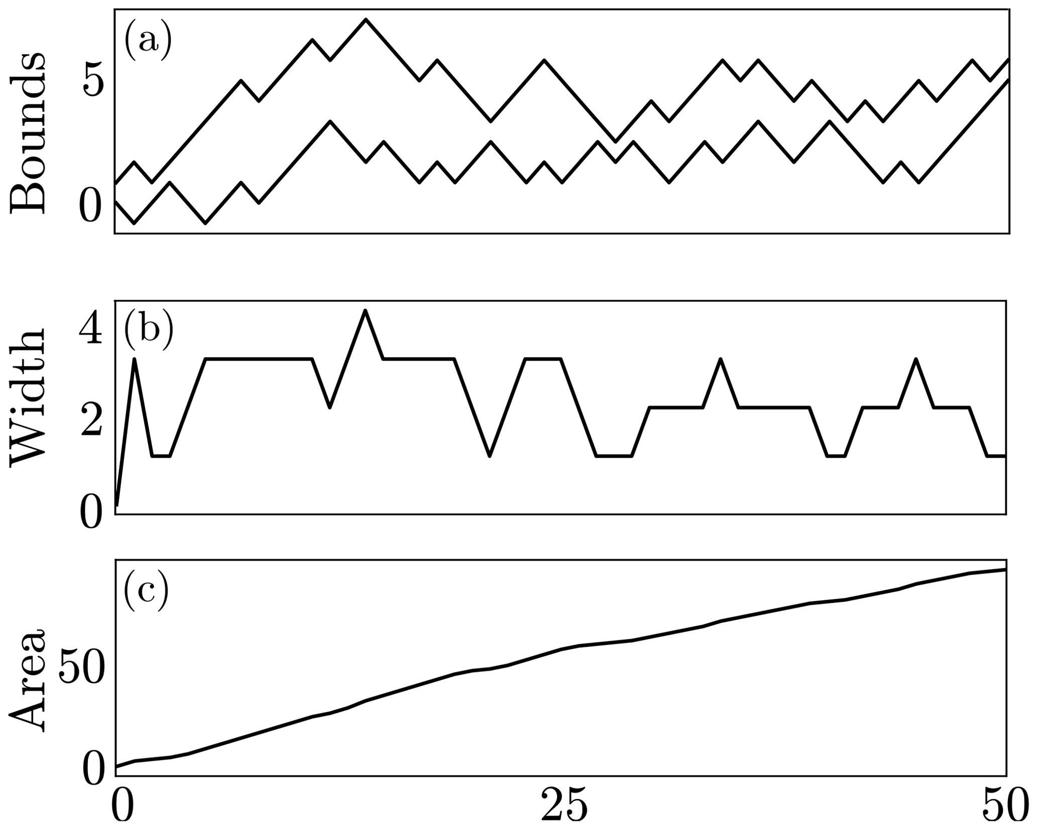
Figure 3 Diagrams showing (a) the positions of two random walks that define the boundary of a watershed, (b) the random walk of w(s), and (c) its integral A(l).

The Scheidegger model serves as an example to determine the properties of b_n, w(s), and A(l). Because it is discrete, it only serves as a useful and simplified guide for the properties of networks. We use the construction of a watershed in the Scheidegger model to inform the spatial evolution of the probability distribution for watershed width, f_w(w,s). The development of such an expression requires definitions of initial conditions, boundary conditions, and transition probabilities. This is the primary utility for the Scheidegger network in our case.

In the Scheidegger model, a new watershed is initiated at s=0 where w=0 by definition. The rill that occupies the watershed begins at s=1. By necessity $w(s=\mathrm{1})>\mathrm{0}$ and because the Scheidegger model is a simplified and discrete model, the width can only be a predefined value, r (L), which is the rill spacing. An initial probability mass function informed by the Scheidegger network is

$$\begin{array}{}\text{(5)}& f_w(r,s=\mathrm{1})=\mathrm{1}.\end{array}$$

Moving down along s, properties of the random walks of b_n completely determine f_w(w;s) and therefore f_A(A|l).

The simple random walks of watershed divides move a distance of $\mathrm{1}/\mathrm{2}r$ left or right with equal probability. The width function over a unit distance can change by $[-r,\mathrm{0},r]$, which occurs with probabilities of $p=[\mathrm{1}/\mathrm{4},\mathrm{1}/\mathrm{2},\mathrm{1}/\mathrm{4}]$ and are the transition probabilities between any two steps. We recognize p as the components of a stencil for an implicit scheme for a central difference solution to linear diffusion (Hornberger and Wiberg, 2004). Recasting this as a diffusion problem requires that we consider a continuous rather than discrete form of f_w(w,s). We restate the initial condition now as a probability density function:

$$\begin{array}{}\text{(6)}& f_w(w,s=\mathrm{1})=\mathit{\delta }(w-r),\end{array}$$

where δ is the dirac function. The boundary conditions reflect the necessity that w(s)>0 for a watershed with length l, where l>s. This forms a fixed boundary condition of $f_w(\mathrm{0},s<l)=\mathrm{0}$. The analytical solution for a diffusion equation with the specified initial and boundary conditions (Carslaw and Jaeger, 1959) is

$$\begin{array}{}\text{(7)}& f_w(w,s)={\displaystyle \frac{\mathrm{2}w}{rs}}{e}^{-\frac{w^{\mathrm{2}}}{rs}}\text{for}s\le l/\mathrm{2},\end{array}$$

which is a Rayleigh distribution. The Rayleigh distribution arises for the problem of the magnitude of the sum of two normally distributed variables (Siddiqui, 1962). Our problem involves the difference between two symmetrically distributed variables, b_n, and thus this result is consistent with previous work.

The boundary condition merits further discussion. We have stated that when w=0, a watershed is closed, which would imply that there is a finite probability of that outcome at all positions. However, the boundary condition that we use prevents watersheds from closing before s=l. We recognize that f_w(w,s) is symmetric about $l/\mathrm{2}$, which allows for us to use our boundary condition for one half of the watershed length (Fig. 4) and reflect this form over the remaining half.

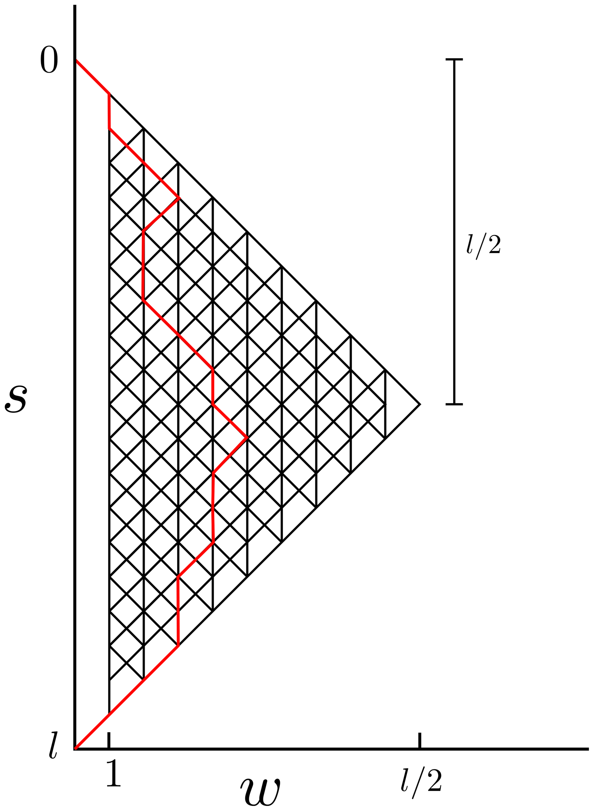
Figure 4 Conceptual diagram showing all possible paths of the width function for a watershed of length, l. The red line is one realization. The ensemble of paths is symmetrical about $l/\mathrm{2}$, and the boundary condition is illustrated by no paths reaching w=0 before l.

The moments of a random walk are key to understanding the distribution of its integral, $A\left(l\right)={\int }_{\mathrm{0}}^{l}w\left(s\right)\mathrm{d}s$. The mean and variance of width from Eq. (7) are

$$\begin{array}{}\text{(8)}& {\displaystyle }& {\displaystyle }{\mathit{\mu }}_w\left(s\right)={\displaystyle \frac{\sqrt{\mathit{\pi }rs}}{\mathrm{2}}},\text{(9)}& {\displaystyle }& {\displaystyle }{\mathit{\sigma }}_w^{\mathrm{2}}\left(s\right)={\displaystyle \frac{\left(\mathrm{4}-\mathit{\pi }\right)r}{\mathrm{4}}}s.\end{array}$$

For an unrestricted Brownian random walk (i.e an infinite domain), Eqs. (8) and (9) contain all of the information required for the distribution of A(l). In that case $f_A(A;l)=\mathcal{N}(\mathrm{0},{\mathit{\sigma }}^{\mathrm{2}}\frac{l^{\mathrm{3}}}{\mathrm{3}})$ (Parzen, 1962), where σ² is the coefficient in Eq. (9). Here, however, the requirement that w(s)>0 imparts finite values for the drift, μ_A(l), changes the scaling between the variance of the random walk and its integral and introduces finite skewness to the distribution. Because the result has finite skewness, more information would be required to determine the form of the distribution. Nonetheless, the first two moments are informative. The mean area involves the integral of μ_w:

$$\begin{array}{}\text{(10)}& {\mathit{\mu }}_A\left(l\right)=\mathrm{2}\underset{\mathrm{0}}{\overset{l/\mathrm{2}}{\int }}{\displaystyle \frac{\sqrt{\mathit{\pi }rs}}{\mathrm{2}}}\mathrm{d}s={\displaystyle \frac{\sqrt{\mathit{\pi }r}}{\mathrm{3}\sqrt{\mathrm{2}}}}{l}^{\mathrm{3}/\mathrm{2}},\end{array}$$

which is a formal expression of Hack's law with A as the dependent variable. Note that the limit of integration and multiplication by 2 reflect the mirrored nature of f_w(w,s) about $l/\mathrm{2}$. We emphasize that Eq. (10) is a complete derivation of Hack's law. Previous work has numerically or empirically demonstrated values of ϕ and m (Hack, 1957; Dodds and Rothman, 2000), where m can range from one-half, for self similar networks, to two-thirds for Scheidegger networks (Maritan et al., 2002; Yi et al., 2018). There is little discussion about the value of ϕ, but it is often determined by fitting distributions or by log–log regression between l and A. Equation (10) represents a formal reasoning for both the values of ϕ and m. Our result is specific for Scheidegger networks; however, a result like Eq. (10) may be obtained if one knows μ_w(s) and the characteristics of w(s).

We now turn to the variance. From Eq. (9) we may obtain ${\mathit{\sigma }}_A^{\mathrm{2}}\left(l\right)$. Once again, if Z(t) is the integral of an unrestricted stochastic process, then ${\mathit{\sigma }}_Z^{\mathrm{2}}\left(t\right)={\mathit{\sigma }}^{\mathrm{2}}{t}^{\mathrm{3}}/\mathrm{3}$ (Parzen, 1962). Here, however, the requirement that w(s)>0 results in a different relationship. We find instead that

$$\begin{array}{}\text{(11)}& {\mathit{\sigma }}_A^{\mathrm{2}}\left(l\right)\approx {\displaystyle \frac{{\mathit{\sigma }}_w^{\mathrm{2}}}{\mathrm{6}}}{\displaystyle \frac{{\left(l-\mathrm{2}\right)}^{\mathrm{3}}}{\mathrm{3}}},\end{array}$$

where the term l−2 satisfies a requirement that a watershed of length 2 has zero variance for the contributing area. The presence of 6 in the denominator lacks a rigorous explanation; however, we expected that ${\mathit{\sigma }}_A^{\mathrm{2}}$ increases at a rate slower than what is typical for unrestricted random walks. We emphasize that this is a semi-empirical result that warrants a stronger theoretical solution. Placing Eq. (9) into Eq. (11), we obtain

$$\begin{array}{}\text{(12)}& {\mathit{\sigma }}_A^{\mathrm{2}}={\displaystyle \frac{\left(\mathrm{4}-\mathit{\pi }\right)r}{\mathrm{72}}}(l_n-\mathrm{2}{)}^{\mathrm{3}}.\end{array}$$

There is good agreement between moments from numerical simulations of random walks and theory (Fig. 5), and these moments become parameters of the distribution f_A(A|l).

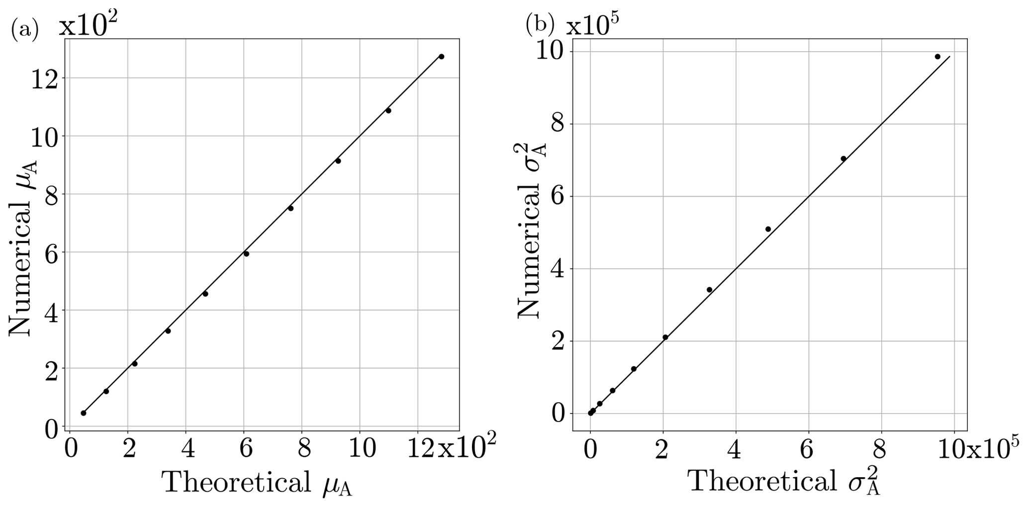
Figure 5 Plots of theoretical versus numerical values for μ_A(l) (a) and ${\mathit{\sigma }}_A^{\mathrm{2}}\left(l\right)$ (b). The 1:1 line is shown in black.

Dodds and Rothman (2000) demonstrate that A(l), given a large l, is distributed as an inverse Gaussian random variable. Inverse Gaussian distributions have a foundation in random walk theory where they describe first-passage processes. However, Dodds and Rothman (2000) state that they identified the inverse Gaussian as the form by postulating it and fitting parameters. Here, we rely on their insight but have developed a basis for the moments and therefore have expressions for the parameters based on the properties of the random walk of w(s). Setting $\mathit{\alpha }=\sqrt{\mathit{\pi }r}/\mathrm{3}\sqrt{\mathrm{2}}$ and $\mathit{\lambda }=(\mathrm{4}-\mathit{\pi })r/\mathrm{72}$ and relaxing the condition that ${\mathit{\sigma }}_A^{\mathrm{2}}(l=\mathrm{2})=\mathrm{0}$, the inverse Gaussian distribution is

$$\begin{array}{}\text{(13)}& f_A\left(A\right|l)=\sqrt{{\displaystyle \frac{{\mathit{\alpha }}^{\mathrm{3}}}{\mathrm{2}\mathit{\pi }\mathit{\lambda }}}}{\displaystyle \frac{l^{\mathrm{3}/\mathrm{4}}}{A^{\mathrm{3}/\mathrm{2}}}}{e}^{-\frac{\mathit{\alpha }(A-\mathit{\alpha }{l}^{\mathrm{3}/\mathrm{2}}{)}^{\mathrm{2}}}{\mathrm{2}\mathit{\lambda }{l}^{\mathrm{3}/\mathrm{2}}A}}.\end{array}$$

As written, Eq. (13) differs from the result obtained by Dodds and Rothman (2000) for two reasons. First, we use a form of Hack's law with area as the dependent variable as opposed to length. Second, they have formed a new variable $z=l{A}^{-\mathrm{2}/\mathrm{3}}$, where we have simply kept the distribution as a function of A.

We numerically simulate the area enclosed by two random walks 100 000 times for watersheds of length 20 and show that the form developed here fits numerical distributions better than the form in Dodds and Rothman (2000) (Fig. 6). Those authors limit their analysis to watersheds that involve more than 500 downslope nodes. It is unclear if there should be a significant difference between large and small watersheds in a Scheidegger model, though we offer it as a possible explanation for the discrepancy between our study and theirs. Now that we have developed f_A(A|l), we move on to the marginal distribution f_A(A;L), where L is a distance from the ridge. We rely on the following relation:

$$\begin{array}{}\text{(14)}& f_A(A;L)=\underset{\mathrm{1}}{\overset{L}{\int }}{f}_l\left(l\right)f_A\left(A\right|l)\mathrm{d}l.\end{array}$$

We now turn to f_l(l).

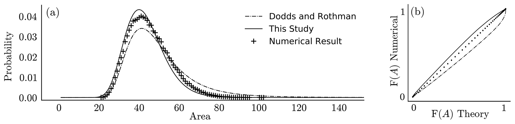
Figure 6 (a) f_A(A|l) according to Dodds and Rothman (2000), this study, and 100 000 numerical simulations of w(s) for watersheds of length 20. (b) Q–Q plot of theory and numerical distributions.

2.4 Watershed length

Watershed lengths are distributed as a power law (Dodds and Rothman, 2000). We write

$$\begin{array}{}\text{(15)}& f_l\left(l\right)={\displaystyle \frac{l^{-\mathrm{3}/\mathrm{2}}}{\mathrm{2}}},\end{array}$$

which is a Pareto distribution with scale parameter 1 and shape parameter $\mathrm{1}/\mathrm{2}$. Lengths of watersheds on hillslopes are necessarily truncated by the hillslope length, L_H. We first consider the distribution of watershed lengths truncated at length L<L_H, which is some downslope position. Though watersheds longer than L are censored, the distribution is not simply truncated, but composed of two populations. The first population contains watersheds that have closed within a length L. The other population contains the watersheds that are open at L and would be longer if L were larger. Proportions of closed and open watersheds respectively are

$$\begin{array}{}\text{(16)}& {\displaystyle }& {\displaystyle }P(l\le L)=F(l\le L)=\mathrm{1}-L^{-\mathrm{1}/\mathrm{2}},\text{(17)}& {\displaystyle }& {\displaystyle }P(l>L)=\mathrm{1}-F(l\le L)=L^{-\mathrm{1}/\mathrm{2}},\end{array}$$

where F(l) is the cumulative probability function. As L increases, the proportion of open watersheds decays. The complete Hack distribution with a maximum length L is a mixture of the two populations and is given by

$$\begin{array}{ll}\text{(18)}& {\displaystyle }f(A,l;L)=& {\displaystyle }P(l\le L)f\left(l\right)f\left(A\right|l\le L)+{\displaystyle }& {\displaystyle }P(l>L)f\left(A\right|l>L).\end{array}$$

Closed watersheds are addressed with the first term on the right-hand side, which combines Eqs. (13), (15), and F_l(l≤L). Open watersheds are addressed with the second term, for which we suggest $f_A\left(A\right|l>L)$ is based on the inverse Gaussian, but the variance and mean differs. For this distribution, we suggest ${\mathit{\alpha }}_{\mathrm{o}}=\sqrt{\mathit{\pi }r}/\mathrm{3}$ and ${\mathit{\lambda }}_o=(\mathrm{4}-\mathit{\pi })r/\mathrm{12}$ because for open watersheds the mirrored character of f_w(w,s) about $l/\mathrm{2}$ does not apply. A functional form for the complete Hack distribution is

$$\begin{array}{}\text{(19)}& \begin{array}{rl}{f}_{A,l}& (A,l;L)={\displaystyle \frac{(\mathrm{1}-L^{-\mathrm{1}/\mathrm{2}})}{\mathrm{2}}}{l}^{-\mathrm{3}/\mathrm{2}}\sqrt{{\displaystyle \frac{{\mathit{\alpha }}^{\mathrm{3}}}{\mathrm{2}\mathit{\pi }\mathit{\lambda }}}}{\displaystyle \frac{l^{\mathrm{3}/\mathrm{4}}}{A^{\mathrm{3}/\mathrm{2}}}}{e}^{-\frac{\mathit{\alpha }(A-\mathit{\alpha }{l}^{\mathrm{3}/\mathrm{2}}{)}^{\mathrm{2}}}{\mathrm{2}\mathit{\lambda }{l}^{\mathrm{3}/\mathrm{2}}A}}\\ & +L^{-\mathrm{1}/\mathrm{2}}\sqrt{{\displaystyle \frac{{\mathit{\alpha }}_{\mathrm{o}}^{\mathrm{3}}}{\mathrm{2}\mathit{\pi }{\mathit{\lambda }}_{\mathrm{o}}}}}{\displaystyle \frac{L^{\mathrm{3}/\mathrm{4}}}{A^{\mathrm{3}/\mathrm{2}}}}{e}^{-\frac{{\mathit{\alpha }}_{\mathrm{o}}(A-{\mathit{\alpha }}_{\mathrm{o}}{L}^{\mathrm{3}/\mathrm{2}}{)}^{\mathrm{2}}}{\mathrm{2}{\mathit{\lambda }}_{\mathrm{o}}{L}^{\mathrm{3}/\mathrm{2}}A}}.\end{array}\end{array}$$

The square root of L grows sufficiently slowly such that the second term is significant on most hillslopes. Our target is the integral of Eq. (19) with respect to l, for which no analytical solution exists, and thus it must be computed numerically. Numerical integration of Eq. (19) reveals an approximate power law distribution, with a notable peak towards the tail which is a result of the second term in Eq. (19). A numerical experiment consisting of 100 000 simulations of w(s) for L=100 reveals a similar shape to the distribution (Fig. 7a). On longer hillslopes probability is shifted towards the tail (Fig. 7b).

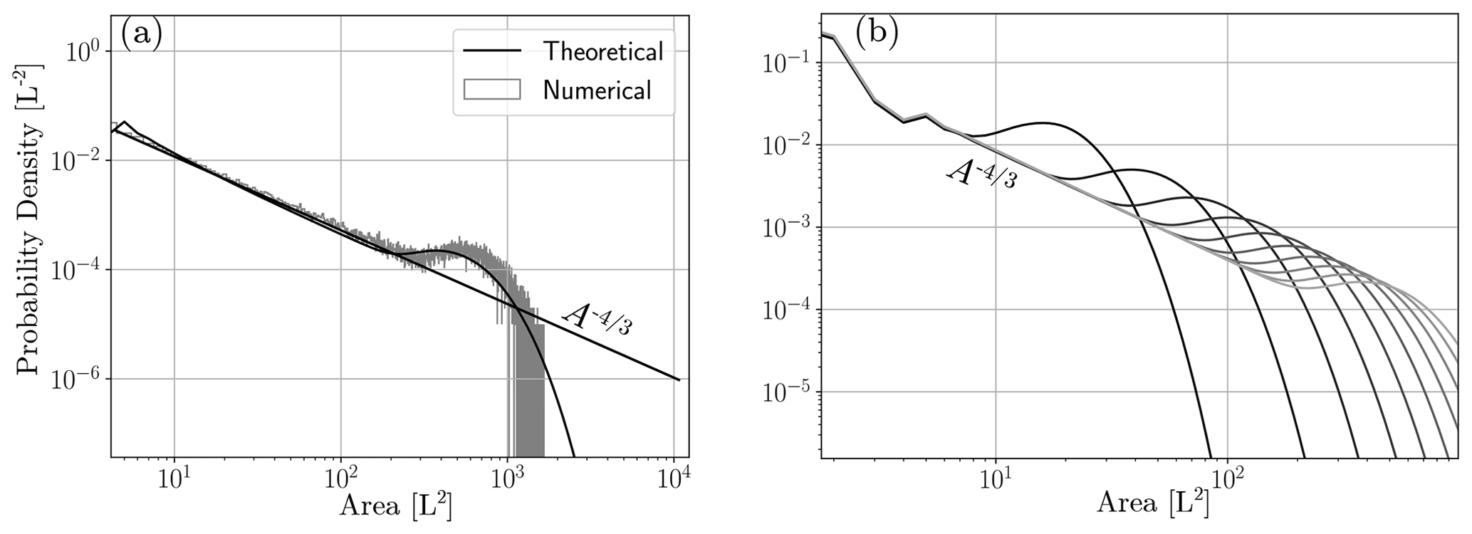
Figure 7 (a) Probability distribution of contributing area on a hillslope according to theory and a numerical exercise of 100 000 simulations of w(s) on a hillslope with 100 levels. (b) Probability distribution of contributing area for hillslopes of increasing length.

The form of f_A(A;L) merits comment. Much of the distribution is characterized by a power law distribution that decays as $A^{-\mathrm{4}/\mathrm{3}}$, which is a result previously highlighted for large Scheidegger networks (Dodds and Rothman, 2000). This power law relationship results from the first term of Eq. (19). However, it is worth noting that even for very long domains, f_A(A;L) will never be entirely monotonic. There will always be some finite probability of a watershed remaining open within that domain. Indeed it is a requirement that at least one watershed be open for a finite rectangular domain of any size. When L is very large, this population may defensibly be neglected and $f_A\left(A\right)\approx A^{-\mathrm{4}/\mathrm{3}}$ is appropriate. On hillslopes, this population is expected to have a significant impact.

We emphasize that f_A(A;L) is the distribution of watershed areas at a position that is a distance L from the hilltop (Fig. 2). Sediment detachment, however, occurs throughout the hillslope according to the magnitude of hydraulic variables. The distribution that informs total hillslope detachment is the complete distribution of contributing area at all points, not just at the terminus of a watershed. To obtain this distribution we sum over all L up to L_h. The distribution is

$$\begin{array}{}\text{(20)}& f_A(A;L_{\mathrm{h}})={\displaystyle \frac{\mathrm{1}}{L_{\mathrm{h}}}}\sum _{L=\mathrm{1}}^{L_{\mathrm{h}}}{f}_A(A;L).\end{array}$$

Numerical computation of Eq. (20) produces a monotonically decaying but truncated distribution of the form $f_A(A;L_{\mathrm{h}})\propto A^{-\mathrm{4}/\mathrm{3}}$ (Fig. 8). As L_h→∞, the truncation disappears. Having demonstrated the form of the distribution of A, we now turn to hydraulic variables.

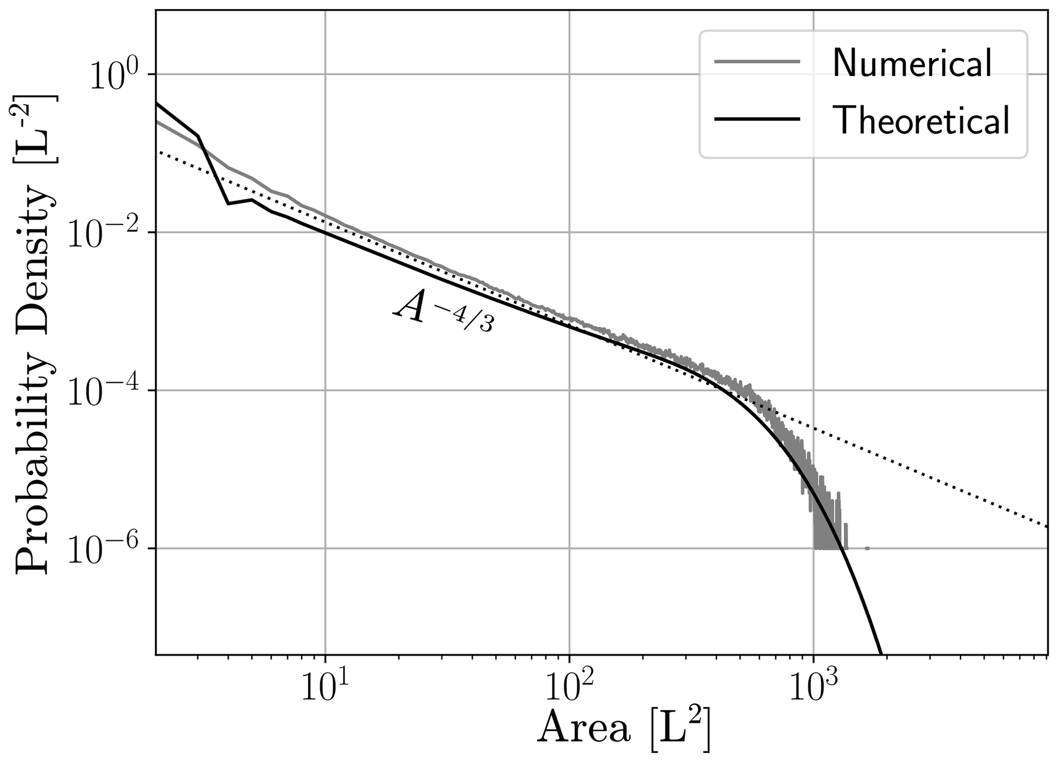
Figure 8 Probability density function of total contributing area on a hillslope with length L_h=100. The dashed line is $A^{-\mathrm{4}/\mathrm{3}}$.

3 Flow properties

We rely on a set of deterministic relationships to extend the theory for area and rill length to hydraulic variables. For a deterministic exponential relationship between two variables x and y

$$\begin{array}{}\text{(21)}& x=\mathit{\xi }{y}^n,\end{array}$$

and y has a known distribution f_y(y), the distribution of x is

$$\begin{array}{}\text{(22)}& f_x\left(x\right)={\displaystyle \frac{\mathrm{1}}{n\mathit{\xi }}}{\left({\displaystyle \frac{x}{\mathit{\xi }}}\right)}^{\mathrm{1}/n-\mathrm{1}}{f}_y\left[{\left({\displaystyle \frac{x}{\mathit{\xi }}}\right)}^{\mathrm{1}/n}\right],\end{array}$$

and we remind the reader that the subscript refers to the functional form of the distribution for y, but the random variable has changed to $(x/\mathit{\xi }{)}^{\mathrm{1}/n}$. Using this relationship, we can write probability functions of discharge, rill width, unit stream power, and shear stress. The task at hand is to generate distributions of these hydraulic variables and perform a Monte Carlo simulation for sediment detachment on hillslopes of different lengths. First, we must generate the distributions from which we will sample. We begin by relating area to water discharge, Q (L³ T⁻¹).

3.1 Hydraulic distributions

At steady-state flow conditions and for uniform runoff, Q=AR, where R (L T⁻¹) is a runoff rate. Because the relationship between A and Q is linear, f_Q(Q;L_h) is the same form of f_A(A;L_h). The distribution of discharge is

$$\begin{array}{}\text{(23)}& f_Q(Q;L_{\mathrm{h}})={\displaystyle \frac{\mathrm{1}}{R}}{f}_A\left({\displaystyle \frac{Q}{R}};L_{\mathrm{h}}\right).\end{array}$$

Obtaining the distribution of discharge is key for hydraulic variables that drive sediment detachment.

Previous work addresses sediment detachment in rilled settings (Hairsine and Rose, 1992; Nearing et al., 1991; 1999; Giminez et al., 2002) which highlights a number of functional forms that relate the volume or mass of detached sediment from the bed to hydraulic variables. Typically researchers suggest that detachment, D_s (L³ T⁻¹), scales as a function of either unit stream power or shear stress. We first consider stream power.

Unit stream power is a measure of the energy expenditure of surface flow on the stream bed and is written as ω=ρgShv, where ρ (M L⁻³) is fluid density, g (L T⁻²) is acceleration due to gravity, S is fluid surface slope, h (L) is flow depth and v is flow velocity (L T⁻¹). Typical models suggest that sediment detaches as a linear function of ω (Govers et al., 2007), though there is evidence that nonlinear relationships exist as well (Nearing et al., 1999). Channel-averaged unit stream power is simple for rectangular or approximately rectangular channel geometries, in which case $\mathit{\omega }=\mathit{\rho }gSQ/r_{\mathrm{w}}$, where r_w (L) is the rill width. Therefore, we first must determine r_w(A) in order to obtain ω(A).

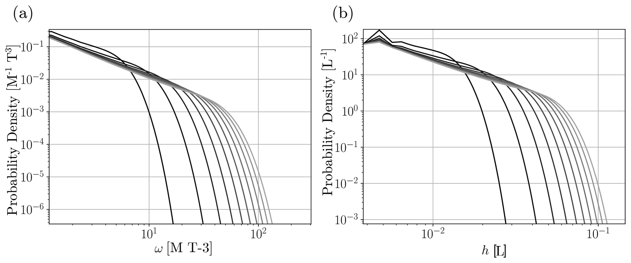
Figure 9 Probability density functions for (a) ω and (b) h for hillslopes with L_h from 10 to 200 by increments of 10. Longer hillslopes are lighter colors. The distribution is not smooth for small values of h because of the discrete calculation.

Previous work demonstrates a relationship between rill width and discharge. Particular values differ between studies, but in general a relationship 〈r_w〉=kQ^γ holds where γ is a dimensionless exponent that typically ranges from 0.3 to 0.5 and k [${\mathrm{L}}^{-\mathrm{2}-\mathit{\gamma }}{\mathrm{T}}^{\mathit{\gamma }}$] is a dimensional coefficient. Gilley et al. (1990) report that k varies over an order of magnitude between 0.2 and 5 depending on the soil type. For simplicity, we set k=1. Torri et al. (2006) present data on rill widths from three different settings and suggest that the value of γ varies from 0.3 to 0.5 for small rills to large gullies. Using this relationship, the unit stream power is

$$\begin{array}{}\text{(24)}& \mathit{\omega }={\displaystyle \frac{\mathit{\rho }gShv}{w_{\mathrm{r}}}}={\displaystyle \frac{\mathit{\rho }gS{Q}^{\mathrm{1}-\mathit{\gamma }}}{k}}.\end{array}$$

Rearranging Eq. (24) to solve for Q and setting $C=k^{\mathrm{1}/(\mathrm{1}-\mathit{\gamma })}(\mathit{\rho }gS{)}^{\mathrm{1}/(\mathit{\gamma }-\mathrm{1})}/R$, we can write the distribution of unit stream power as follows:

$$\begin{array}{}\text{(25)}& f_{\mathit{\omega }}(\mathit{\omega };L_{\mathrm{h}})={\displaystyle \frac{C}{\left(\mathrm{1}-\mathit{\gamma }\right)}}{\mathit{\omega }}^{\frac{\mathit{\gamma }}{\mathrm{1}-\mathit{\gamma }}}{f}_A\left(C{\mathit{\omega }}^{\frac{\mathrm{1}}{\mathrm{1}-\mathit{\gamma }}};L_{\mathrm{h}}\right),\end{array}$$

where again f_A(x;L_h) refers to f_A(A;L_h) where the random variable A has been replaced with x. The general form of the distribution is similar to f_A(A;L_h), though it decays at a different rate that depends on the value of γ (Fig. 9a). The power law portion of the distribution decays as $\sim {\mathit{\omega }}^{-\mathrm{3}/\mathrm{2}}$ for $\mathit{\gamma }=\mathrm{1}/\mathrm{3}$.

Shear stress is another hydraulic variable that is often related to sediment detachment rates (Nearing et al., 1999; Govers et al., 2007). Shear stress is written as $\mathit{\tau }=\mathit{\rho }gSh=\mathit{\omega }/v$. Both h and v are unknown but are related by Manning's equation,

$$\begin{array}{}\text{(26)}& v={\displaystyle \frac{r_{\mathrm{h}}^{\mathrm{2}/\mathrm{3}}{S}^{\mathrm{1}/\mathrm{2}}}{n}},\end{array}$$

where n is Manning's roughness coefficient and $r_{\mathrm{h}}=w_{\mathrm{r}}h/(\mathrm{2}h+w_{\mathrm{r}})$ is the hydraulic radius of the rill. For our planar hillslope, S is uniform so that we only need to solve for h. Setting $v=Q/w_{\mathrm{r}}h$ we can solve for h,

$$\begin{array}{}\text{(27)}& h={\left({\displaystyle \frac{\mathrm{4}}{\mathrm{5}}}\right)}^{\mathrm{2}/\mathrm{3}}{\displaystyle \frac{n}{S^{\mathrm{1}/\mathrm{2}}}}{\displaystyle \frac{{\left(AR\right)}^{\mathrm{1}-\mathrm{5}/\mathrm{3}m}}{k^{\mathrm{5}/\mathrm{3}}}}.\end{array}$$

Following similar steps for f_ω(ω;l), we are able to write out f_h(h,l), which must be numerically integrated to obtain f_h(h;L_h) (Fig. 9b). Again, the distribution is a truncated power law that decays as $h^{-\mathrm{7}/\mathrm{4}}$ when $\mathit{\gamma }=\mathrm{1}/\mathrm{3}$.

A third detachment model involves the concept of transport capacity, wherein the flow accumulates sediment at rates that are inversely proportional to the sediment concentration (Lewis et al., 1994a; Polyakov and Nearing, 2003). As a flow increasingly entrains more sediment downslope, the sediment concentration in the flow asymptotically approaches a maximum value. As typically written, transport capacity is a geometric variable and not a hydraulic one. A common conceptualization is (Polyakov and Nearing, 2003)

$$\begin{array}{}\text{(28)}& {\displaystyle \frac{\mathrm{d}c}{\mathrm{d}s}}=\mathit{\kappa }\left(\mathrm{1}-c/T_{\mathrm{c}}\right),\end{array}$$

where T_c is a maximum concentration that a flow can sustain, κ [L⁻¹] is an empirical coefficient, c is concentration, and s is a position. Here, we use a volumetric form of concentration so that c is dimensionless. We replace s with A and solve for c as follows:

$$\begin{array}{}\text{(29)}& c\left(A\right)=T_{\mathrm{c}}\left(\mathrm{1}-e^{-\frac{\mathit{\kappa }}{T_{\mathrm{c}}}A}\right),\end{array}$$

which may be rearranged to make A(c) such that we may obtain f_A(c;L_h) as we have done for h and ω.

3.2 Sampling hydraulic distributions

We numerically generate samples of ω, τ, and c by inverse transform sampling from f_A(A;L_h) and applying the deterministic relationships laid out above. Inverse transform sampling is a method that may be employed to randomly sample from any probability distribution. The method first generates a random sample of values from a uniform distribution between zero and one. The random sample is then translated to values of the random variables (in this case A) by mapping the values of the random sample to those of the cumulative distribution function which also ranges from zero to one. This is equivalent to sampling from f_A(A;L) but allows for us to do so for any distribution – even those that do not have an analytical expression as is the case here.

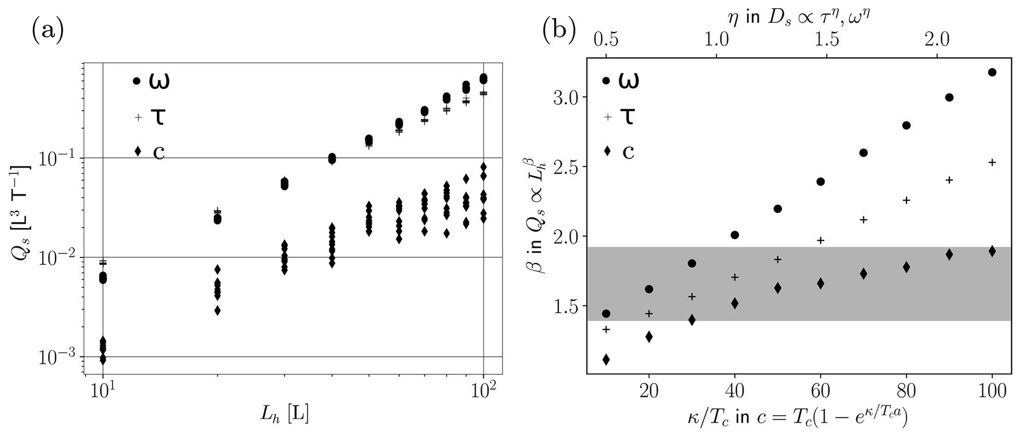
Figure 10 (a) Cumulative volume of detached sediment on hillslopes of length L_h calculated by unit stream power, shear stress, and sediment concentration when $w_{\mathrm{r}}=k{Q}^{\mathrm{1}/\mathrm{3}}$. (b) Best fit power law relationships for different sediment detachment rules (top axis) and rate constants, $\mathit{\kappa }/T_{\mathrm{c}}$, for sediment concentration. The range of observed nonlinear relationships is highlighted in gray.

Inverse transform sampling provides samples of A, and Eqs. (25), (27), and (29) translate it to a sample of hydraulic variables. We consider hillslopes of lengths L_h and with N rills at the first level (L=0). To generate samples for an entire hillslope requires N L_h samples from f_A(A;L_h), which corresponds to N L_h nodes. For each node, we obtain a sample of unit shear stress and stream power. Between nodes, rills accumulate flow in a linear fashion, and we use the average values of τ and ω within a single link. The volume of detached sediment, D_s [L³ T⁻¹] within a link is the area of the channel bed in the link multiplied by the detachment relation:

$$\begin{array}{}\text{(30)}& D_{\mathrm{s}}\propto y^{\mathit{\eta }}{w}_{\mathrm{r}}\mathrm{\Delta }l,\end{array}$$

where y is a placeholder variable for τ and ω and η is an exponent. We then take the sum of all detached sediment over the entire hillslope. Assuming a detachment-limited system and no deposition, the cumulative detachment represents the cumulative volumetric sediment yield, Q_s(L_h).

Sampling for sediment concentration requires a slightly different procedure. Sediment concentration at any given point is the cumulative result of all upslope detachment. Therefore, we only need to know c at the base of the hillslope, and we sample from f_A(A;L_h) N times to obtain samples of Q_s(L_h).

Results from the Monte Carlo simulation demonstrate nonlinear relationships between hillslope length and cumulative sediment yield (Fig. 10a). As the power relationship between detachment and hydraulic variables increases, so too does the exponent that relates hillslope length to cumulative sediment flux (Fig. 10b). The observed range of the power law relationship places $\mathrm{1.4}\le \mathit{\beta }\le \mathrm{1.9}$ and many of our simulations fall within that range. Nearly all simulations that use c with different rate constants fall within the observed range. Detachment models involving τ and ω tend to result in yield–length relationships that are too strongly nonlinear. Our assumption, however, that all detached sediment exits the system is likely a simplification. If deposition were included in this model, it would reduce the nonlinear relationships possibly to near or within the observed range.

The sampling method highlights an interesting sidebar. The theory developed above is for highly idealized networks. There are strict requirements for drainage density, flow direction, rill width, and hillslope shape (rectangular). Under strict conditions, the sum of contributing area at the base of a hillslope must equal the total area of the hillslope. For a hillslope with total width Nr, N samples from f_A(A;L_h) should sum to L_hNr. Such a result only occurs with very small probability and more often the sample hillslope area is only approximately L_hNr. This implies that one or some of our strict requirements have been relaxed. Thus, our samples might represent a hillslope that is not entirely rectangular or where drainage density is not exactly maintained. Such an outcome is a direct result of Monte Carlo simulations and is not novel, but this system highlights the fact that a sampling from an idealized distribution yields a sampled system that is not idealized.

4 Numerical modeling

We demonstrate these distributions with a simplified numerical model that (1) generates topography with a Scheidegger network of rills and (2) simulates steady-state overland flow using Manning's equation and a numerical flow-routing procedure (Pelletier et al., 2005). We simulate steady-state overland flow for a couple of reasons. First, our goal is to demonstrate how the variance of hydraulic variables increases with hillslope length. Steady-state flow conditions accomplish this task. Second, numerical simulations show that, depending on the slope, runoff variables rapidly approach steady-state values within the first 20 min of heavy rainfall and change slowly afterwards (Liu and Singh, 2004). Finally, part of our goal is to illustrate a first-order behavior, and the details of the hydrograph are not considered here.

To generate topography, the numerical model develops a mask of cells that identify the location of rills that satisfy the two rules of Scheidegger networks. Topography is then generated by imposing a uniform lowering rate within the rills and performing linear diffusion on the interrill areas. This leads to approximately parabolic topography in interrill areas. For the theory developed above, we assume rectangular channels so that flow depth is distributed evenly across the channel. In order to best match theory to the condition for numerical modeling, we enforce a rectangular channel of uniform width. Under this condition, the distribution of discharge will remain the same as theory, but hydraulic variables will differ because they depend on channel width. However, w_r is a function of Q and so the numerics can be mapped to theory.

The natural hillslope is from a steep slope in northern Arizona, in the badlands topography of the Painted Desert. The hillslope was scanned using a high-resolution terrestrial lidar scanner, which provides topographic data with 2 cm spatial resolution. The average slope is 1.3 and rill spacing is relatively uniform at about 15 cm (Fig. 11). The slope is sufficiently steep that we anticipate this particular hillslope is detachment limited.

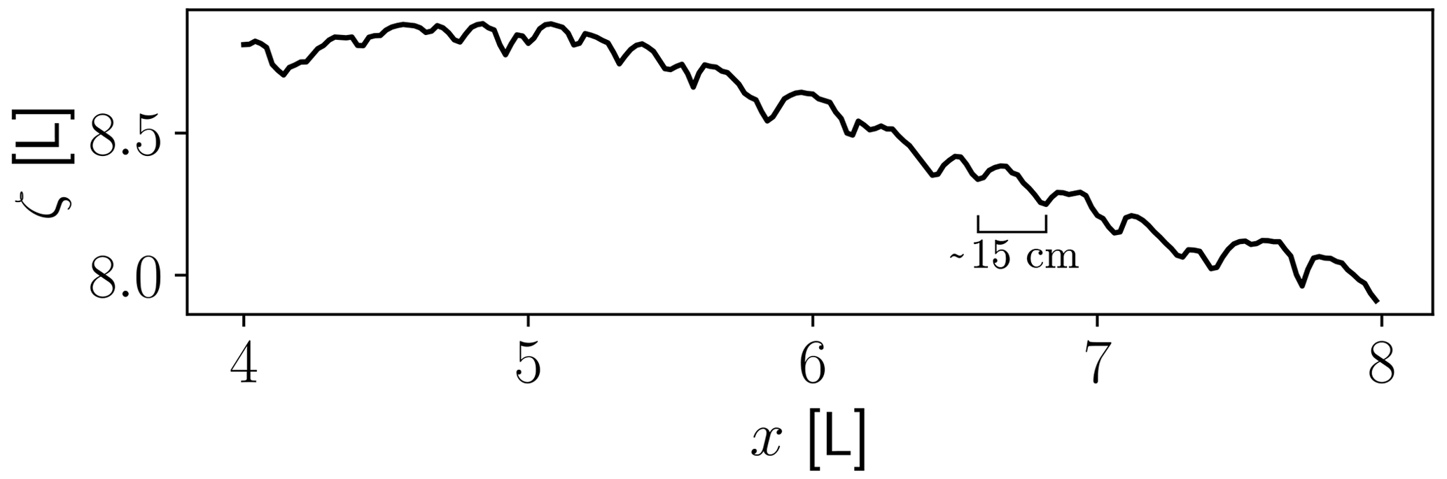
Figure 11 Profile of a section of the natural hillslope highlighting relatively uniform rill spacing.

The numerical modeling routine routes flow using a D-infinity scheme combined with Manning's equation to simulate steady-state conditions. The model iteratively applies a uniform rate of runoff to the surface that is routed downslope according to D-Infinity. For each iteration, Manning's equation solves for depth assuming that it approximates the hydraulic radius (Pelletier, 2008). After each iteration, the depth is updated accordingly and the routine repeats until it approaches a solution to a steady-state configuration of flow depth. This workflow continues until either a threshold of change in depth is reached or a set number of iterations occur. For this work, the threshold for change in average depth between any two iterations is 1 % or about 50 iterations for these hillslopes.

Routing flow down the idealized and natural surfaces reveals steady-state patterns of hydraulic variables (Figs. 12 and 13). Probability distributions from the simulated surface support the theory developed above. The distributions of contributing area and discharge reflect the form of Eqs. (20) and (23) (Fig. 14). The distribution of ω is a deterministic function of Q, and thus the distribution is not shown. Furthermore, because we have specified that our idealized hillslope has a uniform slope, h is the only variable in τ that can change, and thus we plot the distribution of h.

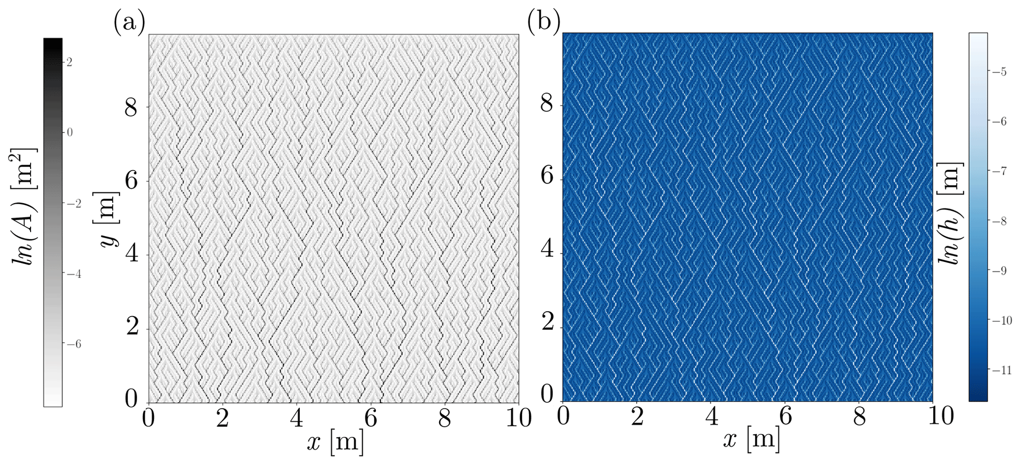
Figure 12 (a) Map of contributing area of half of an idealized hillslope. Color scale is in log scale to make small rills visible and highlight the entire network. (b) Map of steady-state flow depths according to our numerical model for runoff values of 5 cm h⁻¹. This illustrates the results of numerical flow routing. From this result, we calculate exceedance probabilities that compare to theoretical distributions. Color scale is in log scale.

Figure 13 (a) Map of contributing area on half of the hillslope. Color scale is in log scale to make small rills visible and highlight the entire network. (b) Map of steady-state flow depths according to our numerical model. Color scale is in log scale.

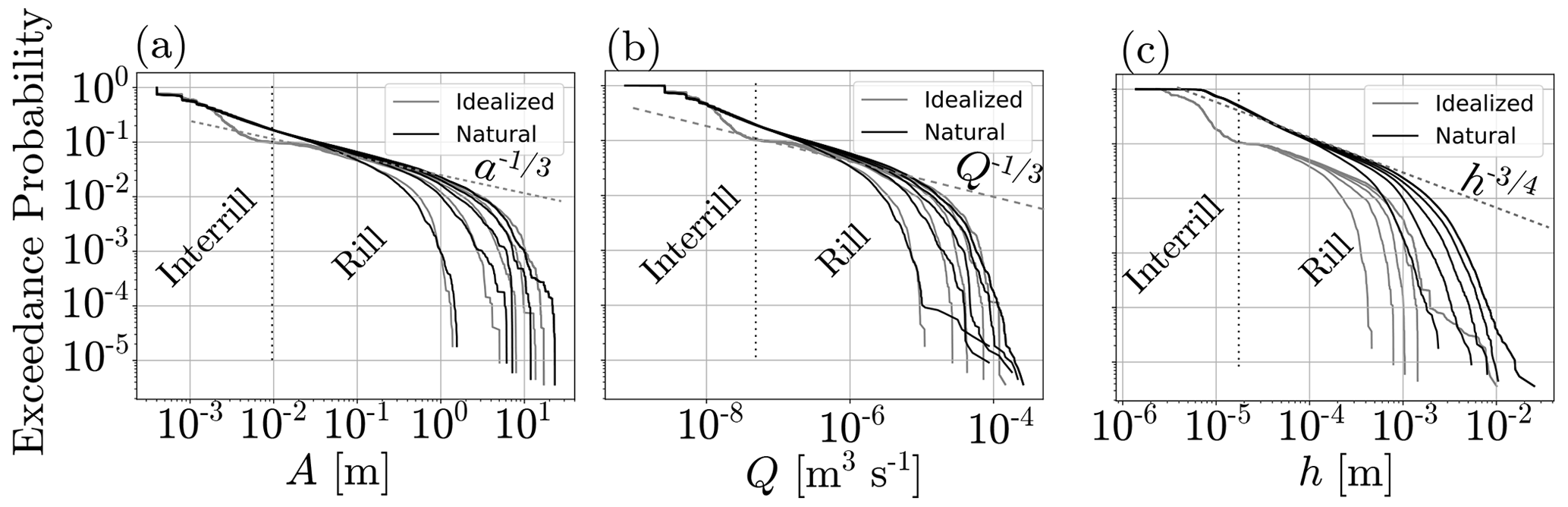
Figure 14 Exceedance probability plots for (a) contributing area, (b) discharge, and (c) flow depth from the hillslope in northern Arizona and an idealized slope. Log–log slopes from theory are plotted on top of the data. The log–log slope in (c) is for $p=\mathrm{1}/\mathrm{3}$ in r_w=kQ^p.

Plots of exceedance probabilities for A, Q, and h (Fig. 14) from the idealized surface reveal similar patterns to theoretical distributions (Fig. 9). As hillslopes lengthen or we sample to progressively lower parts of the hillslope, probability is added to the tail of all empirical distributions. There is good agreement between distributions of geometric variables (A and Q) of the idealized case and the natural one (Fig. 14a and b), which suggests that our theory accurately describes the arrangement of rills. This lends confidence to our Monte Carlo simulation and the implications for the scaling between hillslope length and sediment yield.

Though geometric variables of A and Q match well, there is a notable difference between natural and idealized distributions of h. The forms are again similar; however, the location of truncation for the idealized case is about half an order of magnitude shallower than that for the natural hillslope. There are two reasons for this discrepancy. First, for the idealized case, rill widths are uniform. Second, the natural hillslope is rough and the bed slope contains some noise. Therefore, reductions in slope or the quasi-random narrowing and widening of channels drives an increase in flow depth (Mei et al., 2008). Uncertainty in the spatial patterns of channel width have a significant impact on the distributions. Coupling the work here with a more detailed treatment of w_r may yield interesting results.

5 Discussion

We have contributed to a formal development of the probability functions for topographic variables of A and l for the Scheidegger model. The mathematical steps involve (1) recognizing the width function as a Brownian random walk, (2) developing the description for f_w(w,s), and (3) calculating statistical moments for A based on the moments of w. These steps should be appropriate for many networks; however, they are most applicable to Scheidegger-like networks. By this, we mean networks for which there is a single obvious downslope direction and the surface is roughly planar such that channels do indeed take random walks. This is the case for rilled hillslopes, channels on alluvial fans (McGuire and Pelletier, 2016), and perhaps some large-scale river networks. It is clear that if one can characterize the paths of divide lines as some one-dimensional random walk, then the contributing area becomes the integrated random walk and the steps above hold. Scheidegger networks are simply a special case where the divide lines and the channels share probabilistic properties. This may not be true for other networks.

Though we have developed the moments of the distribution of A, some items remain outstanding. First, in Eq. (11) we have noted that the variance increases at a rate 6 times slower than that of an unrestricted integrated random walk. We suggest this arises from the requirement that the random walk always be positive. However, we currently lack a theoretical explanation for the value of six in the denominator. Further, we have relied on the work of Dodds and Rothman (2000) for the form of the distribution. Although the inverse Gaussian distribution has its foundation in random walk theory, the formal development of the distribution from considering the properties of the random walks remains to be done. We anticipate that the demonstration of f_w(w;s) can contribute towards this because the distribution of a random walk is related to the distribution of its integral.

The theory that we have developed is intended to capture the essence of runoff-driven entrainment. However, it does not consider all processes of entrainment, namely the role of rainfall detachment (Hairsine and Rose, 1992; McGuire et al., 2013). We have not included a theoretical treatment of this process, though it may serve to reduce the nonlinear sediment yield–length relationship. The role of raindrop impacts is greatest on bare surfaces and declines as flow depth increases. In our rilled settings, rain drop detachment will therefore be greatest at the top of the hill and will decline downslope. This is the opposite trend that we see for flow-driven detachment, which only increases downslope. If one were to incorporate raindrop detachment into the theory developed above, it would tend to reduce the nonlinear relationship between sediment yield and hillslope length. We note that Fig. 10 shows nonlinear relationships that are stronger than we typically observe. Therefore, including raindrop impact may contribute to more reasonable scaling relationships. To be clear, this only impacts sediment yield calculated from ω or τ and not concentration, which implicitly incorporates all detachment processes and deposition.

Numerical flow routing highlights the success and challenges of applying the theory developed above. To the first order, the arrangement of rills in a Scheidegger network describes the flow routing on natural hillslopes. This is evident from the distributions of contributing area and discharge. Results shown in Fig. 14a and b highlight that, for both cases, these distributions decay as power laws with exponents close to the theoretical $-\mathrm{4}/\mathrm{3}$. There are, however, distinct differences between them. First, we note that in the natural case, exceedance probabilities R_A(A;L_h) and R_Q(Q;L_h) appear to decay faster than the $A^{-\mathrm{1}/\mathrm{3}}$ that is predicted from theory. This may indicate that the idealized Scheidegger model may not be a perfect description for this network. As mentioned above, other network classes exist, such as OCNs, which may more accurately describe natural networks. However, those networks are not amenable to the type of theory developed above because they lack the clarity in rules for links and nodes of the network. The Scheidegger model serves as a guide to inform probability distributions and provide a basic reasoning for nonlinear relationships. We emphasize that despite the slight difference in power law relationships, the distributions are truncated at remarkably similar locations, which leads to similar scaling relationships.

Another difference is apparent in the distinction between interrill and rill contributions to the distributions. For the idealized case, the distinction between rills and interrills is clear where the interrill portion of the distribution is distinctly not a power law. The same distinction is not clear in the natural slope. We hypothesize that interrill and rill portions do not separate clearly because of the rough topography in the natural hillslope which, even in the interrill areas, tends to focus flow to some degree. The idealized hillslope lacks all roughness, and thus there is no variance in flow for the interrill areas.

We have specified that the mean channel width increases nonlinearly as 〈r_w〉=kQ^γ. For the case where $\mathit{\gamma }=\mathrm{1}/\mathrm{3}$, we expect R_h(h;L_h) to be a truncated power law that decays as $-\mathrm{3}/\mathrm{4}$ for our idealized case. Indeed, this is the slope of exceedance probability for the natural slope shown in Fig. 14c despite slight differences in network geometry. The shape of R_h(h;L_h) depends on γ and the shape of R_A(A;L_h). Assuming that the deterministic relationships hold, we can solve for γ given the slopes of the power law portions of R_A(A;L_h) and R_h(h;L_h). Doing so, we find $\mathrm{1}/\mathrm{5}<\mathit{\gamma }<\mathrm{3}/\mathrm{10}$ for the natural case, which represents the lower range of values from Torri et al. (2006).

There is a legacy of work that describes the behavior of a cohort of particles (Martin et al., 2012; Fathel et al., 2016; Wu et al., 2019; Pierce and Hassan, 2020) that begin their motions at a common location and time. Also referred to as tracer problems, research in this area often targets how that cohort of particles disperses through time. The majority of this work is with regard to transport in fluvial systems where particles take a great number of hops and intervening rest times over timescales that are appropriate for human observation. On hillslopes, particle motion is infrequent and observation of a great number of individual motions involving a cohort of particles is not practical for most settings. Rilled hillslopes, however, offer a unique setting where particles may move frequently. Though an empirical or experimental component of this work remains to be done, Lisle et al. (1998) present probability theory that informs particle dispersion for a rilled setting. However, they consider a single rill that may or may not nonlinearly accumulate flow in the downslope direction. We have demonstrated a probabilistic framework for the rate of flow accumulation downslope, and, in principle, could be used as a basis for further work exploring particle dispersion or residence times on rilled slopes.

6 Conclusions

We have demonstrated probability functions of geometric and hydraulic variables for rilled hillslopes. The theory represents an application of Hack's Law and Hack statistics to hillslopes. The limited space of hillslopes introduces a fundamental difference from the typical application of network scaling arguments (Dodds and Rothman, 2000). We show that the arrangement of rills can lead to nonlinear relationships with sediment detachment that are similar to $Q_{\mathrm{s}}\propto L_{\mathrm{h}}^{\mathit{\beta }}$ that is typically observed in nature (Moore and Burch, 1986; Liu et al., 2000; Govers et al., 2007). Flow-routing numerical simulations on idealized and natural hillslopes demonstrate agreement between geometric probability distributions, which lends merit to the theory.

In pursuing a theoretical form for the distribution of hydraulic variables on hillslopes, we have developed formal expressions for the probability functions of geometric variables. From considering the properties of random walks that define drainage areas, we have developed the joint, conditional, and marginal distributions of watershed length and area. Building on the work in Dodds and Rothman (2000), we have provided a probabilistic basis for the moments of the conditional distribution, f_A(A|l). The first moment of this distribution is the well-known Hack's Law. This result is specific to Scheidegger networks, but the mathematical steps extend to others.

The work presented above is a combination of probability and determinism. We have relied on simple but demonstrable deterministic relationships to extend our understanding of network geometry to hydraulic variables. This represents an attempt to explain the first-order behavior. The theory provides a foundation to consider more detailed and stochastic elements of rill networks such as channel geometry and width variations, variable slope, and the consequences of storm-driven hydrographs.

Appendix A

Symbol	Variable	Units
α	Constant	${\mathrm{L}}^{\mathrm{1}/\mathrm{2}}$
A	Contributing area	L2
b	Lateral position of divide line	L
β	Sediment yield–length exponent	–
c	Sediment concentration	–
Ds	Sediment detachment	L3 T−1
fx(x)	Probability density function for variable x	units of x−1
g	Acceleration due to gravity	L T−2
h	Flow depth	L
k	Discharge–rill width coefficient	${\mathrm{L}}^{-\mathit{\gamma }-\mathrm{2}}{\mathrm{T}}^{-\mathit{\gamma }}$
κ	Sediment concentration coefficient	L−2
l	Channel length of closed watershed	L
L	Downslope distance from ridge	L
Lh	Total hillslope length	L
λ	Constant	L
m	Hack exponent	–
μx	Mean of variable x	units of x
n	Manning's coefficient	${\mathrm{L}}^{\mathrm{1}/\mathrm{3}}\mathrm{T}$
η	Placeholder exponent for detachment models	units vary
ϕ	Hack Coefficient	${\mathrm{L}}^{\mathrm{2}-\mathrm{1}/m}$
ρ	Fluid density	M L−3
γ	Discharge–rill width exponent	–
Qs	Volumetric sediment yield	L3 T−1
Q	Water discharge	L3 T−1
R	Runoff	L T−1
Rx	Exceedance probability for random variable x	–
rh	Hydraulic radius	L
r	Interrill spacing	L
rw	Rill width	L
s	Downslope distance	L
S	Fluid surface slope	–
${\mathit{\sigma }}_x^{\mathrm{2}}$	Variance of variable x	units of x2
θ	Hack coefficient	${\mathrm{L}}^{-m+\mathrm{1}}$
τ	Shear stress	$\mathrm{M}{\mathrm{L}}^{-\mathrm{1}}{\mathrm{T}}^{-\mathrm{3}}$
Tc	Maximum sediment concentration	–
v	Depth-averaged flow velocity	L T−1
ω	Stream power	M L−3
w	Watershed width	L