Coastal change patterns from time series clustering of permanent laser scan data

Sandy coasts are constantly changing environments governed by complex, interacting processes. Permanent laser scanning is a promising technique to monitor such coastal areas and to support analysis of geomorphological deformation processes. This novel technique delivers 3-D representations of the coast at hourly temporal and centimetre spatial resolution and allows us to observe small-scale changes in elevation over extended periods of time. These observations have the potential to improve understanding and modelling of coastal deformation processes. However, to be of use to coastal researchers and coastal management, an efficient way to find and extract deformation processes from the large spatiotemporal data set is needed. To enable automated data mining, we extract time series of surface elevation and use unsupervised learning algorithms to derive a partitioning of the observed area according to change patterns. We compare three well-known clustering algorithms (k-means clustering, agglomerative clustering and density-based spatial clustering of applications with noise; DBSCAN), apply them on the set of time series and identify areas that undergo similar evolution during 1 month. We test if these algorithms fulfil our criteria for suitable clustering on our exemplary data set. The three clustering methods are applied to time series over 30 d extracted from a data set of daily scans covering about 2 km of coast in Kijkduin, the Netherlands. A small section of the beach, where a pile of sand was accumulated by a bulldozer, is used to evaluate the performance of the algorithms against a ground truth. The k-means algorithm and agglomerative clustering deliver similar clusters, and both allow us to identify a fixed number of dominant deformation processes in sandy coastal areas, such as sand accumulation by a bulldozer or erosion in the intertidal area. The level of detail found with these algorithms depends on the choice of the number of clusters k. The DBSCAN algorithm finds clusters for only about 44 % of the area and turns out to be more suitable for the detection of outliers, caused, for example, by temporary objects on the beach. Our study provides a methodology to efficiently mine a spatiotemporal data set for predominant deformation patterns with the associated regions where they occur.

1 Introduction

Coasts are constantly changing environments that are essential to the protection of the hinterland from the effects of climate change and, at the same time, belong to the areas that are most affected by it. Especially long-term and small-scale processes prove difficult to monitor but can have large impacts (Aarninkhof et al., 2019). To improve coastal monitoring and knowledge of coastal deformation processes, a new technique called permanent laser scanning (PLS) (also called continuous laser scanning) based on light detection and ranging (lidar) measurements is available. For this purpose, a laser scanner is mounted on a high building close to the coast in a fixed location acquiring a 3-D scan every hour during several months up to years.

The resulting spatiotemporal data set consists of a series of point cloud representations of a section of the coast. The high temporal resolution and long duration of data acquisition in combination with high spatial resolution (on the order of centimetres) provides a unique opportunity to capture a near-continuous representation of ongoing deformation processes, for example, storm and subsequent recovery, on a section of the coast. As reported by Lazarus and Goldstein (2019), the natural effects of a storm on a typical urban beach can rarely be analysed separately from anthropogenic activities, since in most cases work with bulldozers starts immediately after or even during severe storms. There is a need for the detection and quantification of change processes that influence the geomorphology of the coast, to allow understanding and modelling them, as the reaction of the coast to extreme weather events gains importance (Masselink and Lazarus, 2019). More examples for potential use of such a data set are presented by O'Dea et al. (2019), who use data from a similar setup in Duck, USA.

The PLS data set is large (on the order of hundreds of gigabytes), and to be relevant, the information on deformation processes has to be extracted concisely and efficiently. Currently, there are no automated methods for this purpose and studies focus on one or several two-dimensional cross-sections through the data (for example, O'Dea et al., 2019). The high temporal resolution and long observation period lead to a high-dimensional data set of long time series (i.e. 30 data points up to several thousands). Data mining on high-dimensional data sets can be challenging as discussed, for example, by Zimek et al. (2012). In a first step towards extraction of interesting events and change patterns, we build on the method introduced by Lindenbergh et al. (2019). We use clustering algorithms on time series representing the evolution of topography to group these time series according to their similarity in change pattern and then identify underlying processes. We use clustering (or unsupervised learning) to avoid having to specify the patterns and processes that we are looking for in advance.

One example of spatiotemporal segmentation on our data set from permanent laser scanning was recently developed by Anders et al. (2020). They detected seed points for deformation in time series from permanent laser scanning, to then grow a region affected by the detected change around the seed points with the use of dynamic time-warping distance to spatial neighbours. Dynamic time warping (DTW) is a distance measure between time series that accounts for similarity in patterns even though they might be shifted in time (see, for example, Keogh and Ratanamahatana, 2005). One drawback of this approach is that temporal patterns of interest have to be defined beforehand, and therefore only deformation patterns that are expected can be found. Another approach to model spatiotemporal deformations in point clouds from laser scanning is presented by Harmening and Neuner (2020). Their model assumes that the deformation can be represented by a continuous B-spline surface. This approach could potentially be used to further analyse some of the deformation patterns found in our study but does not allow the exploratory data mining that we are aiming to accomplish. A more general overview of methods to find spatiotemporal patterns in Earth science data was published by Tan et al. (2001) and a continuation of this study was presented by Steinbach et al. (2001). The study of Tan et al. (2001) deals with pre-processing of time series of different variables from satellite data including issues with auto-correlation and seasonality. Steinbach et al. successfully apply a novel clustering technique introduced by Ertöz et al. (2003) to explore spatiotemporal climate data. However, this technique only focuses on contiguous clusters, where all time series are in a close neighbourhood to each other, and does not allow us to find general patterns independent of location.

Time series data sets are also used to assess patterns of agricultural land use by Recuero et al. (2019). For this study, time series of normalized difference vegetation index (NDVI) data have been analysed using auto-correlation values and random forest classification. Benchmark data from an alternative source were needed to train the classifier. Such benchmark data are currently not available in our case. A study by Belgiu and Csillik (2018) used time series from Sentinel-2 satellite data for cropland mapping. They made use of dynamic time-warping classification and showed that in areas with little available reference data for training a classifier, their approach delivers good results in segmentation based on time series' evolution. Also in this case, pre-labelled training data are required. Another approach using expectation-based scan statistics was presented by Neill (2009): to detect spatial patterns in time series from public health data, a statistical method based on expectation values is used. Clusters are formed where the observed values significantly exceed the expectation. The results are promising but depend on the choice of time series analysis method, statistics used and the shape of the search region, which all have to be defined in advance specific to each data set and application. Generally, there is a lack of studies on mining spatiotemporal data for deformation patterns, without using training data or predefined change patterns.

The goal of the present study is to evaluate the application of clustering algorithms on a high-dimensional spatiotemporal data set without specifying deformation patterns in advance. Our objectives in particular are

1. to analyse and compare the limits and advantages of three clustering algorithms for separating and identifying change patterns in high-dimensional spatiotemporal data, and

2. to detect specific deformation on sandy beaches by clustering time series from permanent laser scanning.

We compare the k-means algorithm, agglomerative clustering and the density-based spatial clustering of applications with noise (DBSCAN) algorithm on a PLS data set over 30 d to investigate the effectiveness of the identification of coastal change patterns. All three algorithms are well established and represent three common but different approaches to data clustering. To determine if an algorithm is suitable, we expect that it fulfils the following criteria:

• A majority of the observation area is separated into distinct regions.

• Each cluster shows a change pattern that can be associated with a geomorphic deformation process.

• Time series contained in each cluster roughly follow the mean change pattern.

We use the different clustering approaches on a small area of the beach at the bottom of a footpath, where sand accumulated after a storm, and a bulldozer subsequently cleared the path and formed a pile of sand. We determine the quality of the detection of this process for both algorithms and compare them in terms of standard deviation within the clusters and area of the beach covered by the clustering. We compare and evaluate the resulting clusters using these criteria as a first step towards the development of a method to mine the entire data set from permanent laser scanning for deformation processes.

2 The permanent laser scan data set

The data set from permanent laser scanning is acquired within the CoastScan project at a typical urban beach in Kijkduin, the Netherlands (Vos et al., 2017). For the acquisition, a Riegl VZ-2000 laser scanner was used to scan over a period of 6 months from December 2016 to May 2017. The full data set consists of hourly scans of a section of sandy beach and dunes.

For the present study, a subset of the available data is used to develop the methodology. This subset consists of 30 daily scans taken at low tide over a period of 1 month (January 2017). It covers a section of the beach and dunes in Kijkduin and is displayed in top view in Fig. 1. The area contains a path and stairs leading down to the beach, a paved area in front of the dunes, a fenced in dune area and the sandy beach. It is about 950 m long, 250 m wide and the distance from the scanner to the farthest points on the beach is just below 500 m. For the duration of the experiment, the scanner was mounted on the roof of a hotel just behind the dunes at a height of about 37 m above sea level (as shown in Fig. 2).

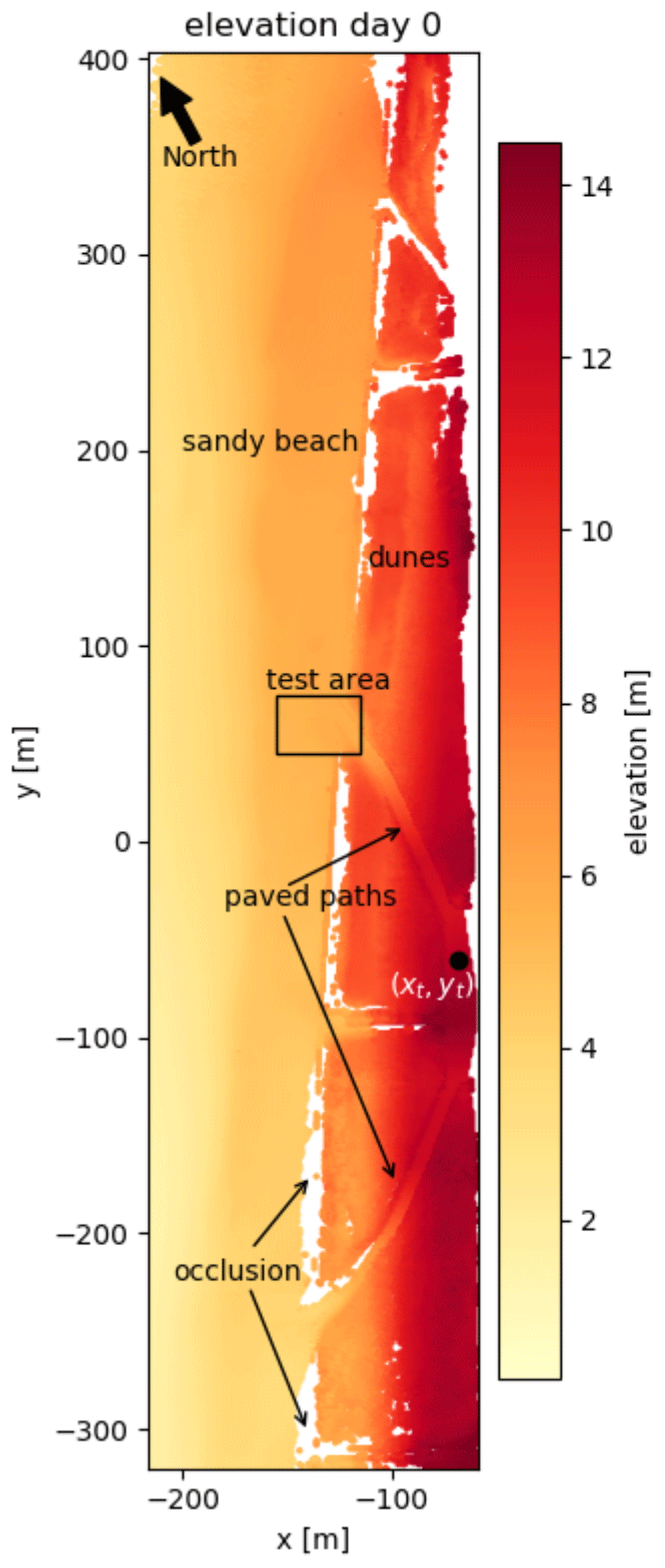
Figure 1 Top view of a point cloud representing the observation area at low tide on 1 January 2017. The laser scanner is located at the origin of the coordinate system (not displayed). The point (x_t,y_t) indicates the location of the time series shown as an example in Fig. 3. The test area, which is discussed in Sect. 3.4, is indicated with a box at the end of the northern path leading to the beach. The paved paths leading to the beach are used as a stable reference surface for the errors reported in Table 1. Parts that are white between the dunes and the sandy beach are gaps in the data due to occlusions caused by the dunes.

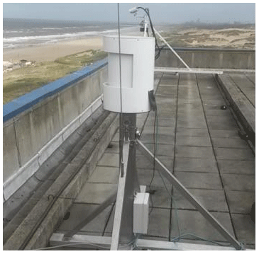
Figure 2 Riegl VZ2000 laser scanner mounted on the roof of a hotel facing the coast of Kijkduin, the Netherlands. The scanner is covered with a protective case to shield it from wind and rain.

The data are extracted from the laser scanner output format and converted into a file that contains xyz coordinates and spherical coordinates for each point. The data are mapped into a local coordinate system, where the origin in x and y directions is at the location of the scanner and the height (z coordinate) corresponds to height above sea level. Since we are interested in relative changes between consecutive scans, we do not transform the data into a georeferenced coordinate system for this analysis.

Each point cloud is chosen to be at the time of lowest tide between 18:00 and 06:00 LT, in order to avoid people and dogs on the beach, with the exception of two instances where only very few scans were available due to maintenance activities. The data from 9 January 2017 are entirely removed from the data set because of poor visibility due to fog. This leads to the 30 d data set, numbered from 0 to 29. Additionally, all points above 14.5 m elevation are removed to filter out points representing the balcony of the hotel and flag posts along the paths. In this way, also a majority of reflections from particles in the air, birds or raindrops are removed. However, some of these particles might still be present at lower heights close to the beach.

Since the data are acquired from a fixed and stable position, we assume that consecutive scans are aligned. Nevertheless, the orientation of the scanner may change slightly due to strong wind, sudden changes in temperature or maintenance activities. The internal inclination sensor of the scanner measures these shifts while it is scanning, and we apply a correction for large deviations (more than 0.01^∘) from the median orientation.

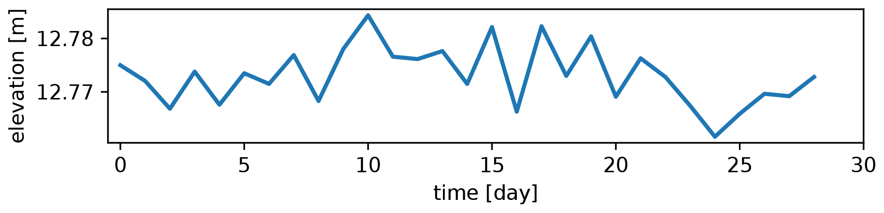
The remaining error in elevation is estimated as the standard error and the 95th percentile of deviations from the mean elevation over all grid cells included in the stable paved area. We chose the stable surface that is part of the paved paths on top of the dunes and leading to the beach in the northern and southern directions as indicated in Fig. 1. This area includes 1653 grid cells with complete time series. The derived mean elevation, standard error and overall 95th percentile of deviations from the mean per time series averaged over the stable area are reported in Table 1. The elevation on average does not deviate more than 1.4 cm from the mean elevation, and 95 % of deviations from the mean elevation are on average below 3.5 cm. An example time series from the stable paved area on top of the dunes (at location (x_t,y_t) marked in Fig. 1) is shown in Fig. 3.

Table 1 Test statistics of the gridded elevation values on the paved area, which is assumed to be stable throughout the observation period of 1 month. Values are calculated per time series and averaged over the entire stable area, which results in mean elevation, standard error and an average 95th percentile of deviations from the mean.

Figure 3 Time series of elevation at location (x_t,y_t) (marked in Fig. 1) on the path that is assumed to be stable throughout the entire month. Elevation varies within less than 2 cm.

3 Methods

To derive coastal deformation processes from clusters based on change patterns, we follow three steps: extraction of time series, clustering of time series with three different algorithms and derivation of geomorphological deformation processes. To cluster time series, the definition of a distance between two time series (or the similarity) is not immediately obvious. We discuss two different options (Euclidean distance and correlation) to define distances between time series with different effects on the clustering results. The rest of this section is organized as follows: we focus on time series extraction in Sect. 3.1, discuss distance metrics for time series (Sect. 3.2), and introduce three clustering algorithms (Sect. 3.3) and our evaluation criteria (Sect. 3.4). The derivation of deformation processes will be discussed with the results (Sect. 4).

3.1 Time series extraction

Time series of surface elevation are extracted from the PLS data set by using a grid in Cartesian xy coordinates. We only use grid cells that contain at least one point for each of the scans.

Before defining a grid on our observed area, we rotate the observation area to make sure that the coastline is parallel to the y axis, as shown in Fig. 1. This ensures that the grid covers the entire observation area efficiently and leaves as few empty cells as possible. Then we generate a regular grid with grid cells of 1 m × 1 m. Time series are generated for each grid cell by taking the median elevation z_i for each grid cell and for each time stamp t_k. That means, per grid cell with centre (x_i,y_i), we have a time series

$$\begin{array}{}\text{(1)}& {\stackrel{\mathrm{̃}}{Z}}_i=\left(z_i\left(t_{\mathrm{1}}\right),\mathrm{\dots }{z}_i\left(t_T\right)\right),\end{array}$$

with the number of time stamps T=30. To make the time series dependent on change patterns, rather than the absolute elevation values, we remove the mean elevation ${\stackrel{\mathrm{‾}}{z}}_i$ of each time series ${\stackrel{\mathrm{̃}}{Z}}_i$. This leads to time series

$$\begin{array}{}\text{(2)}& Z_i=\left(z_i^{\prime }\left(t_{\mathrm{1}}\right),\mathrm{\dots },z_i^{\prime }\left(t_T\right)\right),\end{array}$$

with $z_i^{\prime }\left(t_k\right):=z_i\left(t_k\right)-{\stackrel{\mathrm{‾}}{z}}_i$.

In this way, we extract around 40 000 grid cells that contain complete elevation time series for the entire month. The point density per grid cell varies depending on the distance to the laser scanner. For example, a grid cell on the paved path (at about 80 m range) contains about 40 points (i.e. time series at (x_t,y_t) in Fig. 1), whereas a grid cell located close to the water line, at about 300 m distance from the scanner, may contain around three values. This implies that the median per grid cell is based on more points the closer a grid cell is to the scanner.

3.2 Distance metrics

We consider two different distance metrics for our analysis: the Euclidean distance as the default for the k-means algorithm and agglomerative clustering, and correlation distance for the DBSCAN algorithm.

3.2.1 Euclidean distance

The most common and obvious choice is the Euclidean distance metric defined as

$$\begin{array}{}\text{(3)}& d_{\mathrm{E}}\left(Z_{\mathrm{0}},Z_{\mathrm{1}}\right)=\left|\right|Z_{\mathrm{0}}-Z_{\mathrm{1}}\left|\right|=\sqrt{\sum _{i=\mathrm{1}}^n|Z_{\mathrm{0}i}-Z_{\mathrm{1}i}{|}^{\mathrm{2}}}\end{array}$$

for two time series Z₀ and Z₁ of length n.

3.2.2 Correlation distance

Another well-known distance measure is correlation distance, defined as 1 minus the Pearson correlation coefficient (see, for example, Deza and Deza, 2009). It is a suitable measure of similarity between two time series, when correlation in the data is expected (see Iglesias and Kastner, 2013). Correlation between two time series Z₀ and Z₁ is defined as

$$\begin{array}{}\text{(4)}& \text{Cor}\left(Z_{\mathrm{0}},Z_{\mathrm{1}}\right)=\mathrm{1}-{\displaystyle \frac{\left(Z_{\mathrm{0}}-{\stackrel{\mathrm{‾}}{Z}}_{\mathrm{0}}\right)\cdot \left(Z_{\mathrm{1}}-{\stackrel{\mathrm{‾}}{Z}}_{\mathrm{1}}\right)}{\left|\right|Z_{\mathrm{0}}-{\stackrel{\mathrm{‾}}{Z}}_{\mathrm{0}}\left|\right|\cdot \left|\right|Z_{\mathrm{1}}-{\stackrel{\mathrm{‾}}{Z}}_{\mathrm{1}}\left|\right|}},\end{array}$$

with $\stackrel{\mathrm{‾}}{Z}$ being the mean value of time series Z and $\left|\right|\cdot \left|\right|$ the Euclidean 2-norm as in Eq. (3). We have to note here that correlation cannot compare simple constant time series (leads to division by zeros) and is therefore not a distance metric in the sense of the definition (Deza and Deza, 2009).

3.2.3 Comparison

For a comparison of the two distances for some example time series, see Fig. 4. The example shows that the distance between two time series is not intuitively clear. The use of different distance metrics results in different sorting of distances between the shown pairs of time series. When normalizing all time series (subtracting the mean and scaling by the standard deviation), correlation distance and Euclidean distance are equivalent (as shown, for example, by Deza and Deza, 2009). However, this leads to issues when comparing to a constant time series (with 0 standard deviation).

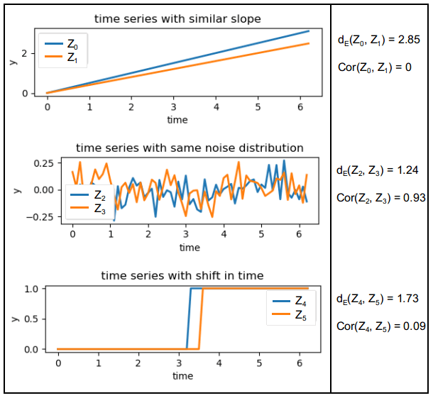
Figure 4 Example of three pairs of time series that are “similar” to each other in different ways. The Euclidean distance would sort the differences as follows: $d_{\mathrm{E}}(Z_{\mathrm{2}},Z_{\mathrm{3}})<d_{\mathrm{E}}(Z_{\mathrm{4}},Z_{\mathrm{5}})<d_{\mathrm{E}}(Z_{\mathrm{0}},Z_{\mathrm{1}})$, whereas according to the correlation distance the order would be $\text{Cor}(Z_{\mathrm{0}},Z_{\mathrm{1}})<\text{Cor}(Z_{\mathrm{2}},Z_{\mathrm{3}})<\text{Cor}(Z_{\mathrm{4}},Z_{\mathrm{5}})$.

Both Euclidean distance and correlation are not taking into account the order of the values within each time series. For example, two identical time series that are shifted in time are seen as “similar” with the correlation distance but not as similar with the Euclidean distance and would not be considered identical by either of them (see Fig. 4). Additionally, neither of the two distance metrics can deal with time series of different lengths or containing gaps.

3.3 Clustering methods

Clustering methods for time series can be divided into two categories: feature-based and raw-data-based approaches (see, for example, Liao, 2005). Feature-based methods first extract relevant features to reduce dimensionality (for example, using Fourier or wavelet transforms) and then form clusters based on these features. They could also be used to deal with gaps in time series. We focus on the raw-data-based approach to not define features in advance and to make sure that no information within the data set is lost. We use three different methods: k-means clustering, agglomerative clustering and DBSCAN. In Fig. 5, an illustration of a partitioning of a simple 2-D data set is shown for each of the three algorithms. The two clusters that can be distinguished in this example have different variances and are grouped differently by each of the algorithms.

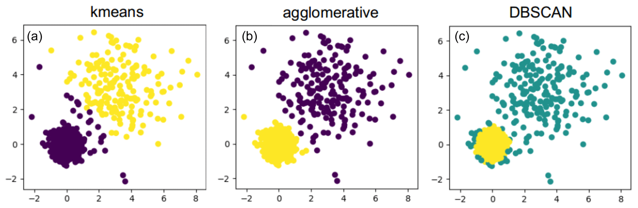
Figure 5 Example of clustering of data with two clusters with different variance: the k-means algorithm separates them but adds a few points in the middle to the purple cluster instead of the yellow one (a). Agglomerative clustering separates both clusters according to their variances (b) and DBSCAN detects the cluster with low variance and high point density (yellow) and discards all other points as outliers (turquoise) (c).

For the implementation of all three algorithms, we make use of the Scikit-learn package in Python (see Pedregosa et al., 2011).

3.3.1 k-means clustering

The k-means algorithm was first introduced in 1955 and is still one of the most widely used clustering methods (Jain, 2010). The algorithm is based on minimizing the sum of all distances between points and centroids over all possible choices of k-cluster centroids $V=\mathit{\{}{v}_{\mathrm{1}},\mathrm{\dots },v_k\mathit{\}}$:

$$\begin{array}{}\text{(5)}& {\text{Min}}_{V}J\left(V\right)=\sum _{j=\mathrm{1}}^k\sum _{x_i\in v_j}\left|\right|x_i-v_j|{|}^{\mathrm{2}},\end{array}$$

with Euclidean distance metric $\left|\right|\cdot \left|\right|$. After the initial choice of k centroids among all points, the following steps are repeated iteratively until the above sum does not change significantly:

1. assign each point to the cluster with the closest centroid;

2. move centroid to the mean of each cluster;

3. calculate the sum of distances over all clusters (Eq. 5).

Note that minimizing the squared sum of distances over all clusters coincides with minimizing the squared sum of all within-cluster variances. The convergence to a local minimum can be shown for the use of Euclidean distance (see, for example, Jain, 2010). The convergence is sped up using so-called k-means++ initialization: after the random selection of the first centroid, all following centroids are chosen based on a probability distribution proportional to their squared distance to the already-defined centroids. In this way, the initial centroids are spread out throughout the data set and the dependence on the random initialization of the cluster centroids is reduced.

There are variations of the k-means algorithm using alternative distance metrics such as the L¹ norm (k-medoids clustering; Park and Jun, 2009); however, the convergence is not always ensured in these cases. Another issue to take into account when considering alternative distance metrics is the definition of the cluster centroids as a mean of time series, which is not automatically defined for any distance metric. For more information on k-means clustering, see Jain (2010), Liao (2005) and the documentation of the Scikit-learn package (Pedregosa et al., 2011).

3.3.2 Agglomerative clustering

Agglomerative clustering is one form of hierarchical clustering: it starts with each point in a separate cluster and iteratively merges clusters together until a certain stopping criterion is met. There are different variations of agglomerative clustering using different input parameter and stopping criteria (see, for example, Liao, 2005, or the documentation of the Scikit-learn package (Pedregosa et al., 2011)). We choose the minimization of the sum of the within-cluster variances using the Euclidean distance metric (Eq. 5, where the centroids v_j are the mean values of the clusters) for a predefined number of clusters k. The algorithm starts with each point in a separate cluster and iteratively repeats the following steps until k clusters are found:

1. Loop through all combinations of clusters:

   • form new clusters by merging two neighbouring clusters into one and

   • calculate the squared sum of distances (Eq. 5) for each combination.

2. Keep clusters with minimal squared sum of distances.

In this way, we use agglomerative clustering with a similar approach to the k-means algorithm, the same optimization criterion with the same input parameter and Euclidean distance measure. We therefore expect similar results. However, this agglomerative clustering can easily be adapted to alternative distance measures and could therefore potentially deal with time series of different lengths or containing gaps.

3.3.3 DBSCAN algorithm

DBSCAN is a classical example of clustering based on the maximal allowed distance to neighbouring points that automatically derives the numbers of clusters from the data. It was introduced in 1996 by Ester et al. (1996) and recently revisited by Schubert et al. (2017). The algorithm is based on dividing all points into core points or non-core points that are close to core points but not surrounded by enough points to be counted as core points. The algorithm needs the maximum allowed distance between points within a cluster (ε) and the minimum number of points per cluster (N_min) as input parameters. These two parameters define a core point: if a point has a neighbourhood of N_min points at ε distance, it is considered a core point. The algorithm consists of the following steps (Schubert et al., 2017):

1. Determine neighbourhood of each point and identify core points.

2. Form clusters out of all neighbouring core points.

3. Loop through all non-core points and add to cluster of neighbouring core point if within maximal distance; otherwise, classify as noise.

In this way, clusters are formed that truly represent a dense collection of “similar” points. Since we choose to use correlation as a distance metric, each cluster will contain correlated time series in our case. All points that cannot be assigned to the neighbourhood of a core point are classified as noise or outliers.

3.4 Evaluation criteria

To determine if an algorithm is suitable, we expect that it fulfils the previously defined criteria:

• A majority of the observation area is separated into distinct regions.

• Each cluster shows a change pattern that can be associated with a geomorphic deformation process.

• Time series contained in each cluster roughly follow the mean change pattern.

In order to establish these criteria, we compare the three clustering algorithms, as well as two choices for the number of clusters k, using the following evaluation methods.

3.4.1 Visual evaluation

The clustered data are visualized in a top view of the observation area, where each point represents the location of a grid cell. Each cluster is associated with its cluster centroid, the mean elevation time series of all time series in the respective cluster. For visualization purposes, we have added the median elevation back to the cluster centroids, even though it is not taken into account during the clustering. We subsequently derive change processes visually from the entire clustered area. We establish which kind of deformation patterns can be distinguished and estimate rates of change in elevation and link them to the underlying process.

3.4.2 Quantitative evaluation

We use the following criteria to compare the respective clustering and grid generation methods quantitatively:

• percentage of entire area clustered;

• minimum and maximum within-cluster variation;

• percentage of correctly identified change in test area with bulldozer work.

The percentage of the area that is clustered differs depending on the algorithm. Especially DBSCAN sorts out points that are too far away (i.e. too dissimilar) from others as noise. This will be measured over the entire observation area. The number of all complete time series counts as 100 %.

Each cluster has a mean centroid time series and all other time series deviate from that to a certain degree. We calculate the average standard deviation over the entire month per cluster and report on the minimum and maximum values out of all realized clusters.

3.4.3 Test area

To allow for a comparison of the clusters with a sort of ground truth, we selected a test area at the bottom of the footpath. In this area, a pile of sand was accumulated by a bulldozer after the entrance to the path was covered with lots of sand during a period of rough weather conditions (8–16 January, corresponding to days 7–14 in our time series), as reported by Anders et al. (2019). We chose two time stamps for illustration and show the elevation before the bulldozer activity at the end of the stormy period on 16 January, after the bulldozer activity on 18 January and the difference between the elevations on these two days in Fig. 6a–c. The area does not change significantly after this event. Within this test area, we classify (manually) each point as “stable” or “with significant change” depending on a change in elevation of more than 5 cm (positive or negative). Then we evaluate for each clustering method if the points that are classified as “with significant change” are in a separate cluster than the “stable” points.

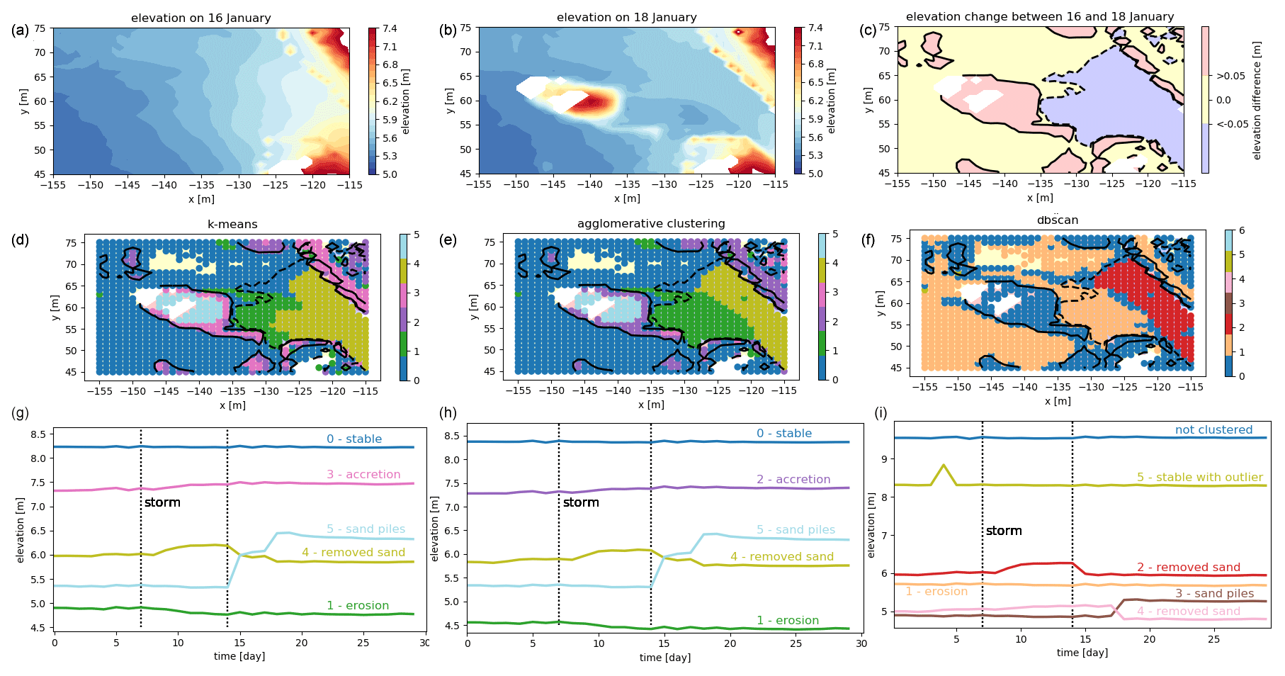
Figure 6 Test area for the comparison of clusters generated with three different algorithms. The test area is located where the northern access path meets the beach (see Fig. 1). (a–c) The elevation in the test area is shown on the day before the bulldozer accumulated a sand pile, when the entrance of the path was covered in sand (a) and after the bulldozer did its job (b). Behind the sand pile, a gap appears in the data (in white), as the sand pile is obstructing the view for the laser scanner. To the right, we show the difference in elevation between 16 and 18 January from a significant level upwards (red) and downwards (blue) (c). (d–f) Test area with significant changes in elevation (contour lines) and points clustered using the k-means algorithm (d), agglomerative clustering (e) and the DBSCAN algorithm (f). The colours of the clustered dots represent the clusters, as shown in Figs. 7, 8 and 9, respectively. (g–i) The corresponding mean time series for each of the relevant clusters are displayed below each of the plots (g, h, i). The dotted lines mark the beginning and end of a stormy period.

The stable cluster consists of cluster 0, the largest cluster when using k=6 for k-means and agglomerative clustering and clusters 0 and 1 combined in the case of k=10 clusters. For evaluating the results of the DBSCAN algorithm, we consider all locations that are not clustered (noise) and points in cluster 1 as the “stable” areas, because the average erosion in cluster 1 is less than 0.15 cm d⁻¹. We do not distinguish if there are different clusters within the category of “with significant change”. However, in Fig. 6, the different clusters can be distinguished by their colours, corresponding to the colours of the clusters shown in subsequent figures (Figs. 7, 8 and 9). We then compare the percentage of correctly classified grid points for the test area, for each of the grid generation and clustering methods.

4 Results

The results are presented in two parts. First, we compare two different choices of the parameter k for the k-means algorithm and for agglomerative clustering. Then, we compare all three clustering methods and evaluate results on the test area, where a bulldozer created a pile of sand (as indicated in Fig. 1) and in terms of percentage of data clustered, standard error within each cluster and physical interpretation of clusters.

4.1 Clustering

For the k-means algorithm and agglomerative clustering, we consider two different values (k=6 and k=10), which are exemplary for a smaller number of clusters and a higher number of clusters.

4.1.1 k-means clustering

With the k-means algorithm, the entire observation area is partitioned. The resulting partition depends on the random initialization. The standard error within each cluster is relatively high, compared to the stable area (see Table 1) and generally increases with the size of the cluster. Even the cluster with the smallest standard error (averaged standard deviation per time series over the clustered area) still shows a standard error of 0.77 m (cluster 5 for k=6). We show the resulting clusters obtained using the k-means algorithm with number of clusters k=6 and k=10. Visual inspection shows that both values lead to good, usable results by partitioning the set of time series into clusters that are small enough to capture geomorphic changes but not too large, which would make them less informative. As displayed in Fig. 7, a large part of the beach is contained in a “stable” cluster when using k=6 (cluster 0, blue). This cluster, as well as some of the others, is split up into several smaller clusters when using k=10. For example, the intertidal zone (i.e. the area that is under water during high tide and exposed during low tide) is eroding mostly during stormy days in the first half of the month. This zone is contained entirely in cluster 1 (green) when using k=6. In the case of k=10, this part is split up into three clusters: one with a similar mean time series (cluster 2, green), one eroding with a pattern similar to cluster 2 but mostly representing sand banks (cluster 3, brown) and one gradually eroding at a low rate over the entire month (cluster 1, orange). It also becomes clear that the sand piles that were generated by bulldozer work at different locations (k=6 cluster 5, light blue) were created on different days (k=10, clusters 8 and 9, yellow and light blue). Some features, like the cleared part of the paths, the sand piles and the intertidal zone, can be distinguished in both cases.

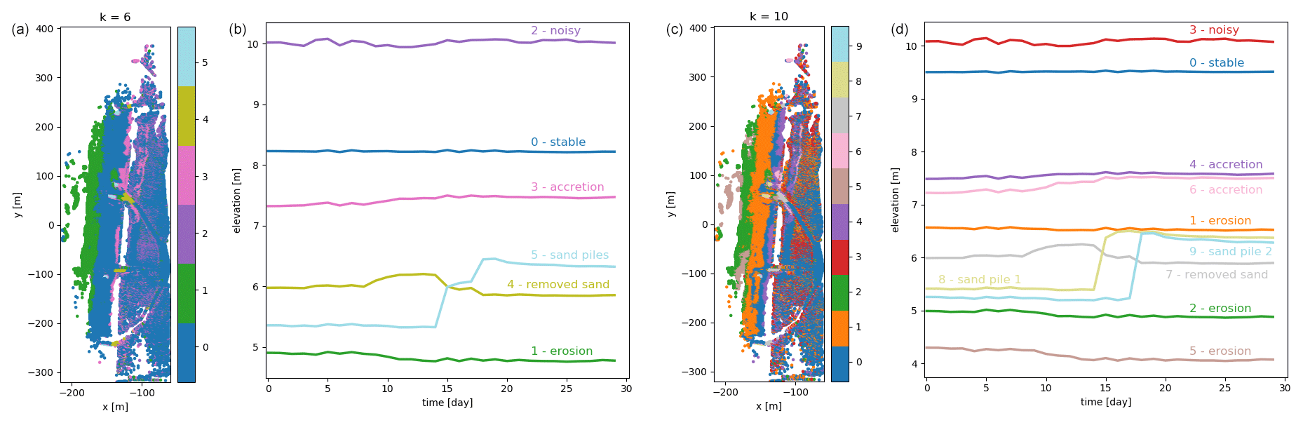
Figure 7 (a, c) Overview of the entire observation area divided into clusters using the k-means algorithm with k=6 (a) and k=10 (c). (b, d) Corresponding cluster centroids for each of the clusters are shown in panels (a) and (c), respectively. By using a larger number of clusters k, more processes become visible, for example, two sand piles (a, b: cluster 5) created on two different days (c, d: clusters 8 and 9). Also the large stable areas (a, b: cluster 0) and slowly accreting areas (a, b: cluster 3) are split up into several clusters: a slightly eroding area (c, d: cluster 3) is split up from the stable part, and the accreting area is split into two (c, d: cluster 4 and cluster 6).

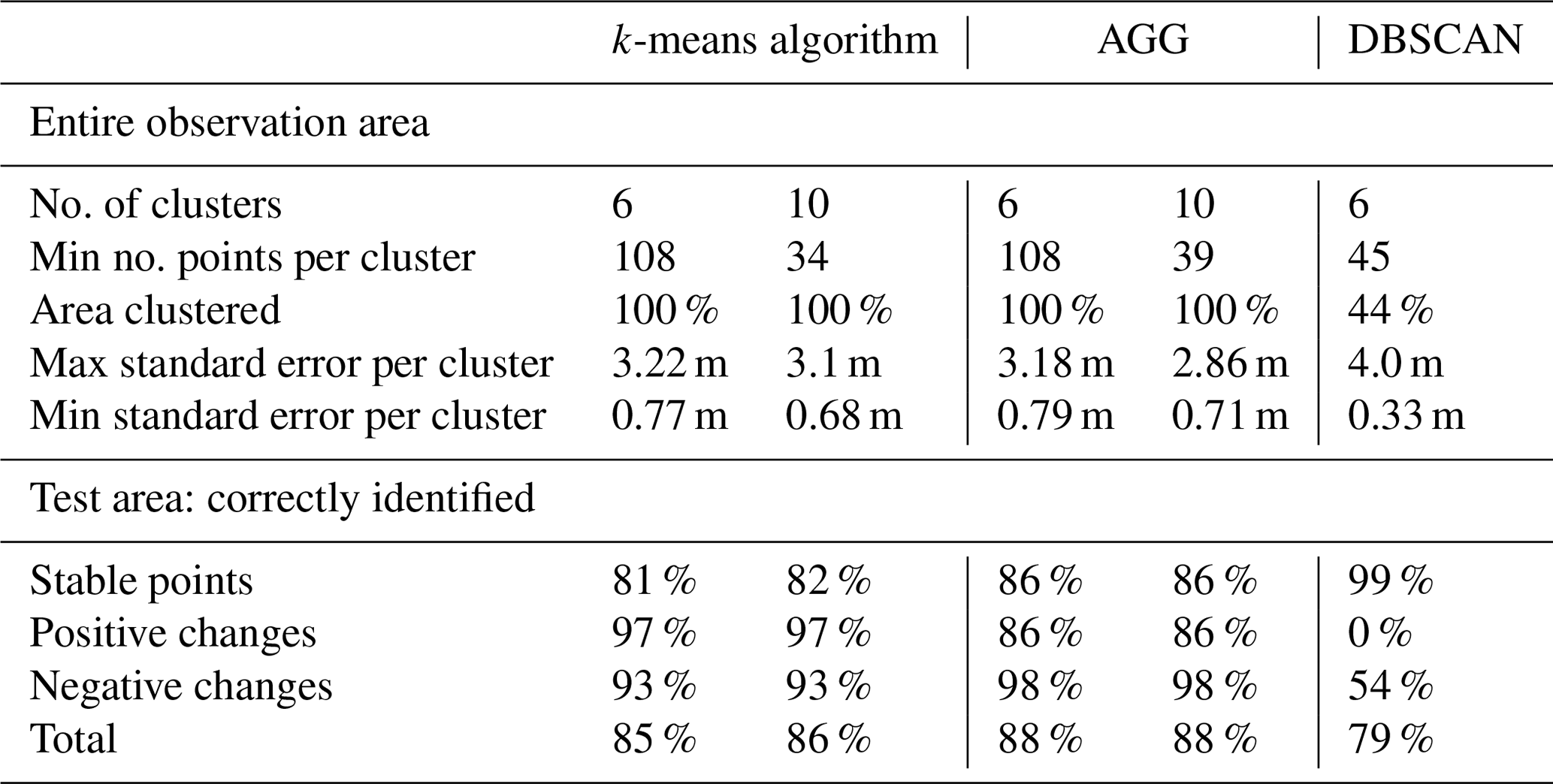
Table 2 Summary of comparison of k-means algorithm, agglomerative clustering (AGG) and DBSCAN algorithm.

On the test area the k-means algorithm correctly classifies about 85 % of points into “stable”, “significant negative change” or “significant positive change” in the case of k=6. However, as can be seen in Fig. 6, a part of the points with negative change are not identified. These clusters are split up further in the case of k=10, which does not influence the results in the test area a lot. A summary of these results is provided in Table 2.

4.1.2 Agglomerative clustering

The agglomerative clustering algorithm is set up, as the k-means algorithm, to find 6 and 10 clusters. It produces results very similar to the clusters found with the k-means algorithm, as can be seen by comparing Figs. 7 and 8 and Fig. 6d and e. Clusters 2 and 3 from agglomerative clustering correspond roughly to clusters 3 and 2 from k-means clustering. The ordering of clusters is according to size, so more time series are considered “noisy” according to k-means clustering, whereas agglomerative clustering assigns more of these time series to the gradually accreting cluster. All other clusters appear to be nearly identical and show similar spatial distributions as well as centroid shapes. The differences between the two choices of the number of clusters k are also very similar.

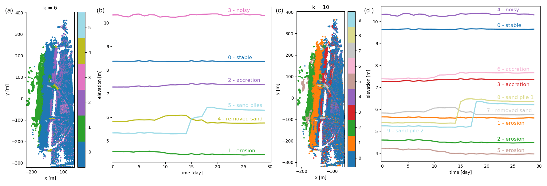
Figure 8 (a, c) Overview of the entire observation area divided into clusters using agglomerative clustering with k=6 (a) and k=10 (c). (b, d) Corresponding cluster centroids for each of the clusters shown in panels (a) and (c), respectively. The clusters are similar to the ones found with k-means clustering.

On the test area, the detection of negative and positive changes is more balanced and leads to an overall score of 88 % correctly identified points. Agglomerative clustering clearly separates the path that was cleared by the bulldozer and identifies it as eroding.

4.1.3 DBSCAN

When we use the DBSCAN algorithm on the same data set, with minimum number of points $N_{min}=\mathrm{30}$ and maximum distance ε=0.05, a large part of the time series (55 %) is classified as noise, meaning that they are not very similar (i.e. not correlated, since we use correlation as distance measure) to any of the other time series. However, they roughly match the combined areas that are identified as stable and noisy by the k-means algorithm (clusters 0 and 2 for k=6). The remaining time series are clustered into six clusters. The standard error within each cluster is generally lower than in the clusters generated with k-means clustering (minimum standard error is 0.33 m) without considering the time series that are classified as noise.

The intertidal zone cannot be separated clearly from the “noise” part of the observation area, nor can we distinguish the stable path area or the upper part of the beach. In the test area, the sand pile is not represented by a separate cluster and positive changes in elevation are not found, which results in an overall worse percentage of correctly identified points. However, two clusters represent areas which are relatively stable throughout the month, except for a sudden peak in elevation on 1 d. These peaks are dominated by a van parking on the path on top of the dunes and people passing by and are not caused by actual deformation; compare Fig. 9.

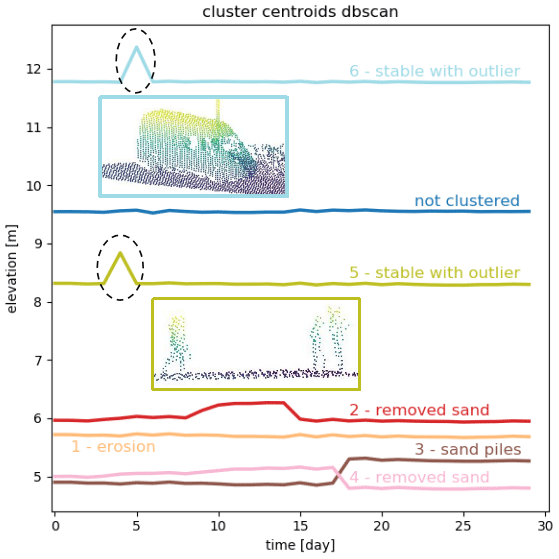
Figure 9 Mean time series per cluster found with the DBSCAN algorithm. Outliers or points that are not clustered are represented by the blue mean time series. The two most prominent time series (clusters 5 and 6, light green and light blue) are located on the path on top of the dunes. The peaks are caused by a group of people and a van, on 5 and 6 January, respectively, illustrated by the point clouds in the middle of the plot.

On the test area, the DBSCAN algorithm performs worse than both other algorithms. In total, 79 % of points are correctly classified into “stable” or “significant negative change”. As stable points, we count in this case all points that are classified either as noise or belonging to cluster 1 (orange). The reason for this is that the mean of all time series that are not clustered appears relatively stable, while cluster 1 describes very slow erosion of less than 0.15 cm d⁻¹. This matches with 99 % of points classified as stable in the ground truth data. However, no single cluster is formed containing only the points where sand is accumulating, even though these clusters are distinguished by the other two algorithms. These points are mixed up with the large cluster of slightly eroding points in cluster 1. We can see in Fig. 6 that the only significant process found in the test area is the cleared path (cluster 2, red).

4.2 Identification of change processes

Considering the clusters found by the k-means algorithm and agglomerative clustering, we can clearly distinguish between time series that represent erosion and accretion with different magnitudes and at different times of the month, as well as a sudden jump in elevation, caused by bulldozer work. In Fig. 10, we show the clusters and associated main process. To give an idea of the magnitude of the most prominent change patterns, we fit straight lines through the mean time series or parts of it (where the slope is steepest) and derived average rates of change in elevation from the estimated slopes. The clusters dominated by erosion close to the water line (clusters 2 and 5) represent the intertidal zone of the beach. The elevation changes in this area are likely caused by the effects of tides and waves. The change rates were partly accelerated during the stormy period in the first half of the month. Accreting areas are mostly at the upper beach, close to the dune foot and on the paths in the dunes (clusters 4, 6 and 7). These areas as well as a large cluster on the upper beach (cluster 1, orange), which undergoes a slight and gradual erosion over the entire month, are likely dominated by aeolian sand transport. The most obvious change process is the sand removed from the entrances of the paths leading to the beach by bulldozer work (cluster 7) and accumulated in piles of sand at four different locations on 2 d (clusters 8 and 9). Points contained in the noisy cluster (cluster 3) are spread out through the dune area, and noise is probably caused by moving vegetation.

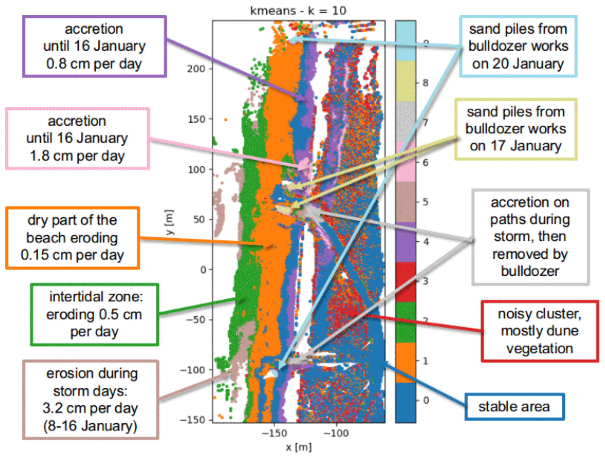
Figure 10 Observation area partitioned into clusters by the k-means algorithm with k=10. The associated processes are annotated with the corresponding colours.

5 Discussion

We successfully applied the presented methods on a data set from permanent laser scanning and demonstrated the identification of deformation processes from the resulting clusters. Here, we discuss our results on distance measures, clustering methods and the choice of their respective input parameters and derivation of change processes.

5.1 Distance measures

Possible distance measures for the use in time series clustering are analysed, among others, by Iglesias and Kastner (2013) and Liao (2005). We use Euclidean distance in combination with the k-means algorithm and agglomerative clustering for our analysis. It has been shown by Keogh and Kasetty (2003) that especially for time series with high dimensions, alternative distance measures rarely outperform Euclidean distance. However, we have to note here that Euclidean distance is affected by the so-called “curse of dimensionality”, which causes a space of long time series (with many dimensions) to be difficult to cluster. The problem with clustering time series in high-dimensional spaces with the k-means algorithm is that Euclidean distance is based on the sum of all pointwise differences. This leads to a space where the variance of the distances decreases with increasing time series length. Therefore, it will be harder to categorize time series as similar, and fewer meaningful clusters will emerge, the more observations we use. This could possibly lead to difficulties when extending these methods to the use of longer time series but does not appear to degrade results on our current data set. For more details on this issue, see Assent (2012), Verleysen and François (2005) and Zimek et al. (2012).

We chose the use of correlation distance with the DBSCAN algorithm, because correlation in principle represents a more intuitive way of comparing time series (see Fig. 4). DBSCAN is based on identification of clusters of high density, which in our case works better using correlation distance instead of Euclidean distance. Using Euclidean distance, there are very few clusters of “very similar” time series and an even larger part of the beach is classified as noise. Only in combination with correlation distance could we derive a set of input parameters for the DBSCAN algorithm to produce relevant results.

Scaling the time series with their respective standard deviations for the use of Euclidean distance would make these two distance measures equivalent. However, this did not improve our results using k-means or agglomerative clustering. Subtle differences within the stable cluster would become prominent in that case, but the larger differences between clusters as we find them without the scaling would be reduced.

Neither of the two distance measures analysed here can deal with gaps in the time series, which would be of great interest to further analyse especially the intertidal area and sand banks. Additionally, both distance measures do not allow us to identify identical elevation patterns that are shifted in time as similar. An alternative distance measure suitable to deal with these issues would be DTW, which accounts for similarity in patterns even though they might be shifted in time (Keogh and Ratanamahatana, 2005). An interpolation method to fill gaps in elevation over short time spans based on surrounding data or a feature-based clustering method could be other alternatives.

5.2 Clustering methods

The use of k-means clustering on elevation time series from the same data set was demonstrated by Lindenbergh et al. (2019) and has shown promising first results. We follow the same approach and, as a comparison, use agglomerative clustering, with the same optimization criterion, distance metric and input parameter. As expected, the results are similar, although agglomerative clustering does not depend on random initialization. It therefore delivers the same result for every run, which is an advantage. Considering our previously defined criteria stating that

• a majority of the observation area is separated into distinct regions,

• each cluster shows a change pattern that can be associated with a geomorphic deformation process, and

• time series contained in each cluster roughly follow the mean change pattern,

both algorithms are suitable and the differences in the resulting clusters are negligible for our specific data set.

However, the computational effort needed to loop through all possible combinations of merging clusters for agglomerative clustering is considerably higher. Of the three algorithms that were used in this study, agglomerative clustering is the only one that regularly ran into memory errors. This is a disadvantage considering the possible extension of our method to a data set with longer time series.

One of the disadvantages of the k-means algorithm and our configuration of agglomerative clustering is that the number of clusters has to be defined in advance. Our choices of k=6 and k=10 clusters both yield promising results but remain somewhat arbitrary, especially without prior knowledge of the data set. A lower number of clusters k (for example, k=6) yields a division of the beach into sections (intertidal zone, dry part of the beach) and highlights the most prominently occurring changes (bulldozer work). When using a larger number of clusters k, several of the previously mentioned clusters are split up again and more detailed processes become visible. The erosion and accretion patterns on the beach appear at different degrees in distinct regions, which is valuable information. Also the sand piles, which appeared in one cluster for k=6, are now split up according to the different days on which they were generated. We consider this possibility to identify and specify anthropogenic-induced change an illustrative example of the influence of the choice of the number of clusters k. We have considered two data-independent methods to determine a suitable value for k: analysis of the overall sum of variances for different values of k and so-called “cluster balance” following the approach of Jung et al. (2003). Neither of them resolved the problem satisfactorily, and we cannot make a generalized recommendation, independent of the application, for the choice of k at this point.

To avoid this issue, we also compare both approaches with the use of the DBSCAN algorithm. It is especially suitable to distinguish anomalies and unexpected patterns in data as demonstrated by Çelik et al. (2011) using temperature time series. To decide which values are most suitable for the two input parameters of the DBSCAN algorithms, we plot the percentage of clustered points and the number of clusters depending on both parameters (see Fig. 11). However, this did not lead to a clear indication of an “optimal” set of parameters. After the trade-off analysis between the number of points in clusters and the number of clusters (not too high, so that the clusters become very small and not too low so that we generate only one big cluster), we chose ε=0.05 and $N_{min}=\mathrm{30}$ by visually inspecting the resulting clusters.

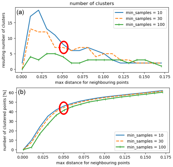
Figure 11 DBSCAN selection of input parameters: number of clusters versus input parameter maximum distance within clusters, and minimum number of points and percentage of total points in clusters (not classified as noise or outliers). The choice of an “optimal” set of parameters is not obvious. We indicate our selection with a red circle in both plots.

An alternative clustering approach for time series based on fuzzy C-means clustering is proposed by Coppi et al. (2010). They develop a method to balance the clustering based on the pattern of time series while keeping an approximate spatial homogeneity of the clusters. This approach was successfully applied to time series from socioeconomic indicators and could be adapted for our purpose. It could potentially improve detection of features like sand bars or bulldozer work but not distinguish moving vegetation in the dunes as our current approach does.

A similar approach would be to use our clustering results and identified change patterns as input to the region-growing approach of Anders et al. (2020). In this way, we could combine advantages of both methods by making the identification of the corresponding regions for each distinct deformation pattern more exact, without having to define possible deformation patterns in advance.

5.3 Derivation of change processes

As shown in Fig. 10, we identified change processes from the clusters generated by the k-means algorithm. Agglomerative clustering shows similar clusters and therefore yields similar results. Each centroid representing the mean time series of the k-means clusters shows a distinct change pattern (see Figs. 7 and 8), which allows us to conclude on a predominant deformation process. By fitting a straight line through the mean time series, or part of it, we estimated the slope corresponding to the average rate of change in elevation. Associating the centroids with the location and spatial spread of the clusters allows us to derive the main cause for the respective deformations. In some cases, extra information or an external source of validation data would be useful to verify the origin of the process. This will be taken into account for future studies. The location of the clusters and, for example, the steep rise of the mean time series representing the sand piles allow for the conclusion that the cause of this sudden accretion is anthropogenic. The information found by Anders et al. (2019) for the research on their study confirms the coinciding bulldozer work. The derived average rates of change in elevation allow for the possibility to derive mass budgets to quantify volume changes over specific amounts of time from our data, showing a possible application of our method that is of large scientific interest (see, for example, de Schipper et al., 2016).

The DBSCAN algorithm successfully identifies parts of the beach that are dominated by a prominent peak in the time series (caused by a van and a small group of people). Out of the three algorithms that we compare, it is most sensitive to these outliers in the form of people or temporary objects in the data. It was not our goal for this study to detect people or objects on the beach, but this ability could be a useful application of the DBSCAN algorithm to filter the data for outliers in a pre-processing step.

6 Conclusions

We compared three different clustering algorithms (k-means clustering, agglomerative clustering and DBSCAN) on a subset of a large time series data set from permanent laser scanning on a sandy urban beach. We successfully separated the observed beach and dune area according to their deformation patterns. Each cluster, described by the mean time series, is associated with a specific process (such as bulldozer work, tidal erosion) or surface property (for example, moving vegetation cover).

The most promising results are found using k-means and agglomerative clustering, which both correctly classify between 85 % and 88 % of time series in our test area. However, they both need the input of the number of clusters we are looking for, and agglomerative clustering is computationally expensive. DBSCAN turned out to be more suitable for the identification of outliers or unnatural occurring changes in elevation due to temporary objects or people in the observed area.

Our key findings are summarized as follows:

1. Both k-means and agglomerative clustering fulfil our criteria for a suitable method to cluster time series from permanent laser scanning.

2. Predominant deformation patterns of sandy beaches are detected automatically and without prior knowledge using these methods. The level of detail of the detected deformation processes is enhanced with increasing number of clusters k.

3. Change processes on sandy beaches, which are associated with a specific region and time span, are detected in a spatiotemporal data set from permanent laser scanning with the presented methods.

Our results demonstrate a successful method to mine a spatiotemporal data set from permanent laser scanning for predominant change patterns. The method is suitable for the application in an automated processing chain to derive deformation patterns and regions of interest from a large spatiotemporal data set. It allows such a data set to be partitioned in space and time according to specific research questions into phenomena, such as the interaction of human activities and natural sand transport during storms, recovery periods after a storm event or the formation of sand banks. The presented methods enable the use of an extensive time series data set from permanent laser scanning to support the research on long-term and small-scale processes on sandy beaches and improve analysis and modelling of these processes. In this way, we expect to contribute to an improved understanding and management of these vulnerable coastal areas.