Size, shape and orientation matter: fast and semi-automatic measurement of grain geometries from 3D point clouds

The grain-scale morphology and size distribution of sediments are important factors controlling the erosion efficiency, sediment transport and the aquatic ecosystem quality. In turn, characterizing the spatial evolution of grain size and shape can help understand the dynamics of erosion and sediment transport in coastal, hillslope and fluvial environments. However, the size distribution of sediments is generally assessed using insufficiently representative field measurements, and determining the grain-scale shape of sediments remains a real challenge in geomorphology. Here we determine the size distribution and grain-scale shape of sediments located in coastal and river environments with a new methodology based on the segmentation and geometric fitting of 3D point clouds. Point cloud segmentation of individual grains is performed using a watershed algorithm applied here to 3D point clouds. Once the grains are segmented into several sub-clouds, each grain-scale morphology is determined by fitting a 3D geometrical model applied to each sub-cloud. If different geometrical models can be tested, this study focuses mostly on ellipsoids to describe the geometry of grains. G3Point is a semi-automatic approach that requires a trial-and-error approach to determine the best combination of parameter values. Validation of the results is performed either by comparing the obtained size distribution to independent measurements (e.g., hand measurements) or by visually inspecting the quality of the segmented grains. The main benefits of this semi-automatic and non-destructive method are that it provides access to (1) an un-biased estimate of surface grain-size distribution on a large range of scales, from centimeters to meters; (2) a very large number of data, mostly limited by the number of grains in the point cloud data set; (3) the 3D morphology of grains, in turn allowing the development of new metrics that characterize the size and shape of grains; and (4) the in situ orientation and organization of grains. The main limit of this method is that it is only able to detect grains with a characteristic size significantly greater than the resolution of the point cloud.

1 Introduction

Rock particles or grains are characterized by a large range of size, from clays to large boulders, and a diverse variety of shape and angularity, from spherical or ellipsoidal to cubic or polyhedral (e.g., Blott and Pye, 2008; Domokos et al., 2014; 2020). Grains form initially by fragmentation or chemical weathering, transforming a cohesive rock mass into a granular material. The initial size or shape distributions are controlled by fragmentation, weathering processes and structure of the rock mass (e.g., fracture density and orientation, mineral size) (e.g., Molnar et al., 2007; Garzanti et al., 2008; Sklar et al., 2017; DiBiase et al., 2018; Neely and DiBiase, 2020; Verdian et al., 2021). These initial distributions then evolve due to the action of geomorphological processes, including attrition, chipping, abrasion, fragmentation, chemical weathering and transport of grains by wind, river flow, avalanches along hillslopes, and sea waves and currents (e.g., Attal and Lavé, 2006; 2009; Domokos et al., 2014; Miller et al., 2014; Várkonyi et al., 2016; Novák-Szabó et al., 2018; Marc et al., 2021). Grains are also found at the surface of other planetary bodies or asteroids (Burke et al., 2021) and offer unique constraints on their surface conditions. A striking example is the use of the shape of grains to reconstruct the transport history of pebbles on Mars (Szabo et al., 2015). Moreover, the in situ orientation of grains found in deposits can also provide information on the paleo-flow conditions during sediment deposition (e.g., Johansson, 1963; Rust, 1972).

The distributions of grain size, shape and orientation impact the dynamics of fluvial and sedimentary environments. At the scale of rivers, the size of the sediments strongly controls the mobility of alluvial grains and their incipient threshold of motion (e.g., Shields, 1936), the timescale required to mobilize landslide-driven sediments (e.g., Croissant et al., 2017), the rate of river bedrock incision through the tool-and-cover effect (Sklar and Dietrich, 2004), the width of river channels (e.g., Finnegan et al., 2007; Baynes et al., 2020), and the rate of knickpoint propagation (Cook et al., 2013). At the scale of a sedimentary basin, the size of grains influences the stratigraphy of the basin together with the chemical and mechanical properties of the sediment (e.g., Armitage et al., 2011). Grain size, shape and orientation in riverbeds are also key factors for aquatic habitats (e.g., Kondolf and Wolman, 1993; Riebe et al., 2014), for water and nutrient exchange through the hyporheic zone (e.g., Tonina and Buffington, 2009), and even for river hydraulics by impacting basal friction (e.g., Hodge et al., 2009).

Despite the ubiquitous role of grain geometry on landscape properties and dynamics, and its potential to constrain paleo-conditions on Earth and other planetary bodies, robustly documenting the 3D geometry of grains and their statistical distributions in natural environments remains a challenge. Sampling the grain-size distribution of the sediments lying at the surface of a riverbed is often done by the grid-by-number method (Wolman, 1954). This method measures the diameter of a pre-defined number of grains, generally greater than 100. The grid-by-number method is simple to implement and is regarded as directly similar to a volumetric sampling (see Bunte and Abt, 2001; and references therein). It is therefore widely used in the field (e.g., D'Arcy et al., 2017; Guerit et al., 2014; 2018; Chen et al., 2018; Roda-Bodula et al., 2018; Watkins et al., 2020; Baynes et al., 2020). However, samples are often taken over a few square meters and thus lead to inherent representativeness and statistical biases associated with the operator, the grain sampling strategy, the measurements themselves and with the choice of the diameter to be measured. Collecting a data set can be extremely time-consuming, especially when many grains have to be measured to be statistically significant (Rice and Church, 1996; Green, 2003; Eaton et al., 2019; Purinton and Bookhagen, 2021). Measurements are also partly destructive (i.e., grains are moved), which generally leads to information being lost on grain orientation and exact location.

These issues have led to the development of alternative methods based on image analysis to characterize large areas in a manageable amount of time. Object-based and statistically based approaches have been developed to characterize grain-size distributions from pictures or 3D data. The first approach (the so-called “photo sieving”) measures each grain or a number of selected grains on a picture (e.g., Bunte and Abt, 2001). Several algorithms now exist to perform these measurements manually on an image (Roduit, 2008). Because this manual procedure can be time-consuming, (semi-)automatic procedures have been implemented to recognize grains from pictures (Butler et al., 2001; Graham et al., 2005a, b; Detert and Weitbrecht, 2012; Buscombe et al., 2013; Langhammer et al., 2017; Carbonneau et al., 2018; Purinton and Bookhagen, 2019) Machine learning approaches are being developed to support grain segmentation for images (Soloy et al., 2020). However, these methods are still time-consuming as they require the manual labeling of a large number of grains. The second approach is based on image-texture analyses and aims to correlate some statistical properties of images with grain sizes of the study site (Buscombe and Masselink, 2009; Buscombe et al., 2010; Rubin, 2004; Carbonneau et al., 2004). Similarly, 3D approaches empirically relating bed roughness measured on high-resolution topographic data can be implemented to infer the grain-size distribution from locally calibrated relationships (e.g., Rychkov et al., 2012; Westoby et al., 2015; Woodget and Austrums, 2017; Vazquez-Tarrio et al., 2017; Pearson et al., 2017; Groom et al., 2018; Detert et al., 2018). These approaches considerably reduce the time spent in the field, efficiently increase the sampling density and coverage, and are non-destructive. Yet, post-processing remains time-consuming, and these methods are inherently limited to the 2D measurement of the apparent axis of individual grains (Graham et al., 2010) or to empirical local correlations with little generalization capability and limited potential to fully explore the 3D geometry of individual grains.

The last decade has seen a steep growth in the use of high-resolution 3D topographic data in Earth Sciences and geomorphology, obtained by lidar measurements and photogrammetry (e.g., Schneider et al., 2015; Westoby et al., 2012; Leduc et al., 2019). The resulting 3D point clouds offer unprecedented access to landscape heterogeneities and to landscape temporal evolution (e.g., Hodge et al., 2009; Leyland et al., 2017; Beer et al., 2017; Bernard et al., 2021). The accessibility of 3D point clouds, obtained from terrestrial, drone and airborne data, and their ability to capture object geometries robustly and accurately in 3D at various scales represent a timely opportunity to develop point-cloud-based methods for the issue of grain-size measurement. Building on this opportunity, Chen et al. (2020) recently developed a deep-learning workflow to segment grains based on structure-from-motion (SfM) data. Walicka and Pfeifer (2022) also successfully applied a DBSCAN (density-based spatial clustering of applications with noise, see Ester et al., 1996) algorithm to segment grains.

In this paper, we develop another efficient and semi-automatic approach, entitled G3Point (standing for “Granulometry from 3D Point clouds”), to measure grain size, shape and orientation using 3D point clouds. G3Point is a purely geometric algorithm, which in turn does not rely on the a priori training of a neural network on thousands or more grains which is required in Chen et al. (2020). Indeed, the associated workflow consists of the 3D segmentation of individual grains using a type of watershed algorithm, the geometrical description of individual grains using 3D ellipsoidal models, and the description of the 3D geometry of the grain population using statistical distributions. G3Point can be characterized as a semi-automatic approach as it is based on several parameters which can be optimized by a trial-and-error approach. Moreover, validation of the obtained results is performed either by comparing the obtained size distribution to independent measurements (e.g., hand measurements) or by visually inspecting the quality of the segmented grains. After describing the new method, we test it against lab and natural controlled experiments (e.g., riverbeds and beaches), considering point clouds obtained from SfM, to check its ability to robustly capture the 3D geometry and size of grains, independently constrained by hand measurements.

Figure 1 Overview of the G3Point algorithm showing the main series of functions (center) and the results (top and bottom figures). Each main function is described in detail in the Method section.

2 Method

G3Point is a Matlab program which aims at measuring the size, shape and orientation of a large number of individual grains as detected from 3D point clouds describing the topography of surfaces covered by sediments. The main functions of G3Point are described in the following and Fig. 1. Compared to 2D digital elevation models (DEMs), where elevation z is defined as a function of the horizontal coordinates (x, y), 3D point clouds can include several points located at the same horizontal position (e.g., the face above and below a grain), allowing a better description of geomorphological features such as grains. In the following, we assume that the considered point cloud is already denoised and cleaned of any geometrical feature not corresponding to pebbles. These features include trees, trunks, vegetation, the water surface, human-made objects and patches of fine grains (i.e., smaller than the minimal detected grain size). Several efficient algorithms are available to perform the denoising task (e.g., Lague and Brodu, 2013). We also assume that the point cloud surface, over the region of interest (i.e., generally an area of a few tens of square meters, what we later refer to as the “patch scale”), is relatively planar with its normal oriented vertically upward. We provide functions to denoise and reorient the point cloud accordingly. We also assume that in most cases vertically stacked rocks cannot be individually segmented.

Figure 2 Three-dimensional view of the point cloud, its segmentation into individual grains and the fit ellipsoids. (a) Initial point cloud with the color map indicating the elevation of the points. (b) Initial segmentation of the point cloud into individual grains performed with a modified watershed algorithm using the steepest upward slope criterion to route water. (c) Segmentation after merging close grains together. (d) Ellipsoid fit to each individual grain identified in panel (c) is represented by colored lines (same color as in panel c) over the point cloud (black dots). Color in panels (a), (b) and (c) indicates the label of the grains (i.e., one color per grain). Red dots in panels (a) and (b) indicate the location of the summit point of each grain. (e) Picture showing the location of the point cloud surface, bounded by a red polygon, relative to the Otira river.

To illustrate the method, we apply it to a point cloud of an active alluvial riverbed, of an area of ∼40 m², acquired in 2011 with a terrestrial lidar scanner (Leica ScanStation 2) along the Otira River in New Zealand (Fig. 2) and already featured in Brodu and Lague (2012). The subset of this point cloud that we use in the following is made of ∼10⁵ points with an average point density of ∼2.410³ pt m⁻² and was obtained after a single scan (Fig. 2a). Because it was acquired after a single scan and therefore misses a significant surface area for each visible grain, this point cloud is not optimal to obtain robust information on grain size. However, it represents a valuable test to check the ability of G3Point.

2.1 Initial segmentation: from a global point cloud to individual grains using a watershed algorithm

The segmentation of the point clouds into sub-point clouds representing individual grains uses a single flow algorithm based on the steepest slope criterion (O'Callaghan and Mark, 1984). This algorithm is generally used to route water and identify watersheds on 2D DEMs. It uses the steepest slope criterion to route water between neighborhood points until reaching a local topographic minimum, which corresponds to the outlet of the watershed. Each watershed is therefore described by a directed acyclic graph which associates each point of the point cloud with its outlet node through a single flow path (e.g., Schwanghart and Scherler, 2014). To perform the watershed segmentation, we use the Fastscape algorithm as it offers a fast solution to order points along the steepest water flow path (Braun and Willett, 2013). For each node i, Fastscape defines a receiver node, corresponding to the neighborhood node leading to the steepest slope (i.e., that therefore would receive water when defining a flow topology), and donor nodes, corresponding to neighborhood nodes that give water to node i. Starting from each outlet node, a stack of nodes is built by recursively adding the donor nodes to the stack until reaching nodes without donors. The list of nodes in each stack therefore defines a watershed associated with one outlet node. This algorithm, designed for regular grids, can be readily adapted to irregular grids, such as 3D point clouds, as long as the neighborhood nodes of each node are known. We use here the k-nearest neighbors algorithm, using 3D Euclidean distances, to identify the neighborhood nodes. The parameter k controls the “neighborhood scale”, which varies locally based on the spatial density of points (Fig. A1a). For the point cloud of the Otira River, k was taken as equal to 20 as this provides a good solution to grain segmentation. We provide some guidelines on how to choose a suitable value of k in the Supplement (Fig. S1).

To identify grains instead of watersheds, the single flow algorithm is modified by using the criterion of the steepest slope upward instead of the steepest slope downward to route water. In other words, water is routed from a point to its steepest upward neighbor, which is associated with the maximum value of $\mathrm{\Delta }z/{\left(\mathrm{\Delta }{x}^{\mathrm{2}}+\mathrm{\Delta }{y}^{\mathrm{2}}\right)}^{\mathrm{1}/\mathrm{2}}$, with Δx, Δy and Δz the distance along x, y and z between the considered point and its k-nearest neighbors. Using this approach, each grain should be identified by a single watershed, with the outlet corresponding to the summit of the grain. For the Otira River, the initial segmentation identifies 772 grains (Fig. 2b), and their set of points are associated with a unique label. This segmentation approach is relatively simple to implement, and the topology of a grain can be simplified to the position of its summit (red dots in Fig. 2b). Moreover, this segmentation method is fast as it takes ∼0.1 or ∼1 s of CPU time for ∼10⁵ or ∼10⁶ points, respectively, on a laptop with 32 GB of RAM and an Intel i9 CPU of eight cores with a clock speed of 2.4 GHz. We emphasize that this algorithm is not intended to provide an accurate description of hydrological flow over a point cloud as in Rheinwalt et al. (2019) but simply to provide a fast segmentation of the point cloud. This algorithm only imposes one spatial scale: the theoretical minimum grain diameter which can be segmented, i.e., the local neighborhood scale. This scale can lead to under-segmentation of small grains, when their number of points is lower than or of the same order as the k parameter. Except for the neighborhood scale, no other scale is introduced, and the algorithm can identify grains of varying size. However, results show that this watershed segmentation approach also leads to a global over-segmentation of grains. Indeed, grains can exhibit several local maxima, due to the geometry of the grain (i.e., angularity) or to a rough surface or to potential data noise, leading to a grain being over-segmented (Fig. 2b). Over-segmentation is a classical issue for algorithms dedicated to grain segmentation in 2D (e.g., Purinton et al., 2019; Purinton and Bookhagen, 2021) or 3D.

2.2 Correcting from over-segmentation by merging grains

Correcting over-segmentation is not a trivial task due to the large range of grain sizes. Mostly because of this issue, classical clustering approaches such as hierarchical clustering or DBSCAN (e.g., Esther et al., 1996) proved ineffective to solving this issue. Moreover, approaches that use all the points in the point cloud can lead to a longer computational time, which might become prohibitive for large point clouds. Here, we develop an approach which makes use of the properties of the segmented watersheds, which associate grains (i.e., watersheds) to their unique summit points (i.e., outlets) and to their border nodes (i.e., crests). We combine three criteria (Fig. A1b) to decide if a pair of grains (ij) should be merged into a single grain.

• Criterion 1: the distance d_ij between two summit points should be smaller than the sum of the characteristic radius of the two grains. Using a criterion based on a single scale to decide whether two grains should be merged would be problematic due to the large range of grain size. We therefore use the drainage area A at the summit node (i.e., outlet), which receives water from all the points sharing the same label, to determine a characteristic scale or grain radius $l_i={\left(A_i/\mathit{\pi }\right)}^{\mathrm{1}/\mathrm{2}}$. The criterion to merge the pair of grains (ij) together is therefore d_ij<C_F(l_i+l_j), with C_F a factor that we take generally to be equal to 0.5–1. These values were obtained after several trial-and-error tests.

• Criterion 2: grains i and j should be neighbors (i.e., at least one of the points of grain i belongs to the k neighbors of one point of grain j and vice versa).

• Criterion 3: the 3D angle between the normals of the crest points of grains i and j should be small. Orientation of the normal is computed by taking the normal of the best-fitting local plane to the k-nearest neighbors of the considered point. For each of the crest nodes of grain i, the sum of the 3D angle between its normal and the normal of its neighbors belonging to grain j is computed. This operation is performed for every crest point of grains i and j, and then a mean 3D angle is determined. The criterion to merge the grains is that their mean 3D angle is lower than a threshold α that we take as equal to 60^∘ for the point cloud of the Otira River. This last criterion prevents grains that are separated by a clear change in surface orientation from being merged.

A pair of grains (ij) is merged if, and only if, these three criteria are respected. Due to the low number of grains compared to the number of points in the point cloud, this step is also fast (i.e., $\sim \mathrm{0.1}-\mathrm{1}$ or $\sim \mathrm{1}-\mathrm{10}$ s of CPU time on a laptop for ∼10⁵ or ∼10⁶ points, respectively). The results show that many labels, suffering from over-segmentation and describing a single grain, were effectively merged by applying this test, leaving only 657 labels or grains instead of 772 (Fig. 2c). Overall, the resulting segmentation looks qualitatively good, even if some grains still suffer from over-segmentation while a limited number of labels now suffer from under-segmentation and include more than one grain. We provide some guidelines on how to choose suitable values of C_F and α in the Supplement (Fig. S2).

2.3 Segmentation cleaning operations

To increase the quality of the segmentation, we offer optional routines to perform several post-segmentation operations (Fig. A1c):

• applying Criterion 3 only, which merges a pair of grains if the 3D angle between their normal, computed on the common border, is lower than a threshold β. The objective is mostly to merge small grains, resulting from the initial over-segmentation due to grain local maxima, with large ones.

• cleaning the segmentation by removing grains with less than n_min points. This number of points should be greater than or equal to k, the number of nearest neighbors, and greater than or equal to 10, regarded as the strict minimum number of points required to fit an ellipsoid (i.e., number of parameters of an ellipsoid). However, larger values of n_min should be favored to reduce the uncertainty in the resulting ellipsoidal model.

• removing flattish or over-elongated grains, as they generally do not correspond to individual grains but to clusters of fine grains with a characteristic size much lower than the typical point spacing of classical point clouds or to improperly segmented grains. To detect flattish or over-elongated grains, we perform a singular value decomposition (SVD) over the 3D coordinates of each of the sub-point clouds. If a grain has a minimum or an intermediate singular value divided by its maximum singular value (i.e., the axis ratio between the intermediate or minimum dimension of the 3D labeled point cloud and its maximum dimension) lower than a threshold, ∅_flat or 2∅_flat, then this grain is considered flattish or over-elongated, respectively, and removed from the segmentation. Values of ∅_flat<0.1 were found to be suitable in this study, even if natural settings with very flat (e.g., as found for slate grains) or elongated grains should probably consider smaller values.

In the example shown in Fig. 2, the segmentation was not cleaned. We provide some guidelines on how to choose suitable values of β, n_min and ∅_flat in the Supplement (Fig. S3).

2.4 Geometrical modeling: 3D ellipsoidal fitting of grains

Once the grains are segmented and labeled, the following phase consists of the 3D geometrical description of each grain, particularly their size and orientation. A strong constraint results from the fact that only an unknown fraction of the upper surface of the segmented grains (i.e., the visible part of the grain) is topographically described by the point cloud. This prevents us from directly using the point cloud to describe each grain and measure their sizes and orientations. Instead, we rely on geometrical models to represent each grain. The simplest 3D geometrical model to describe a grain is the ellipsoidal model. Two strategies are adopted to describe the geometry of a grain with an ellipsoidal model: fitting an ellipsoid or determining its ellipsoid of inertia.

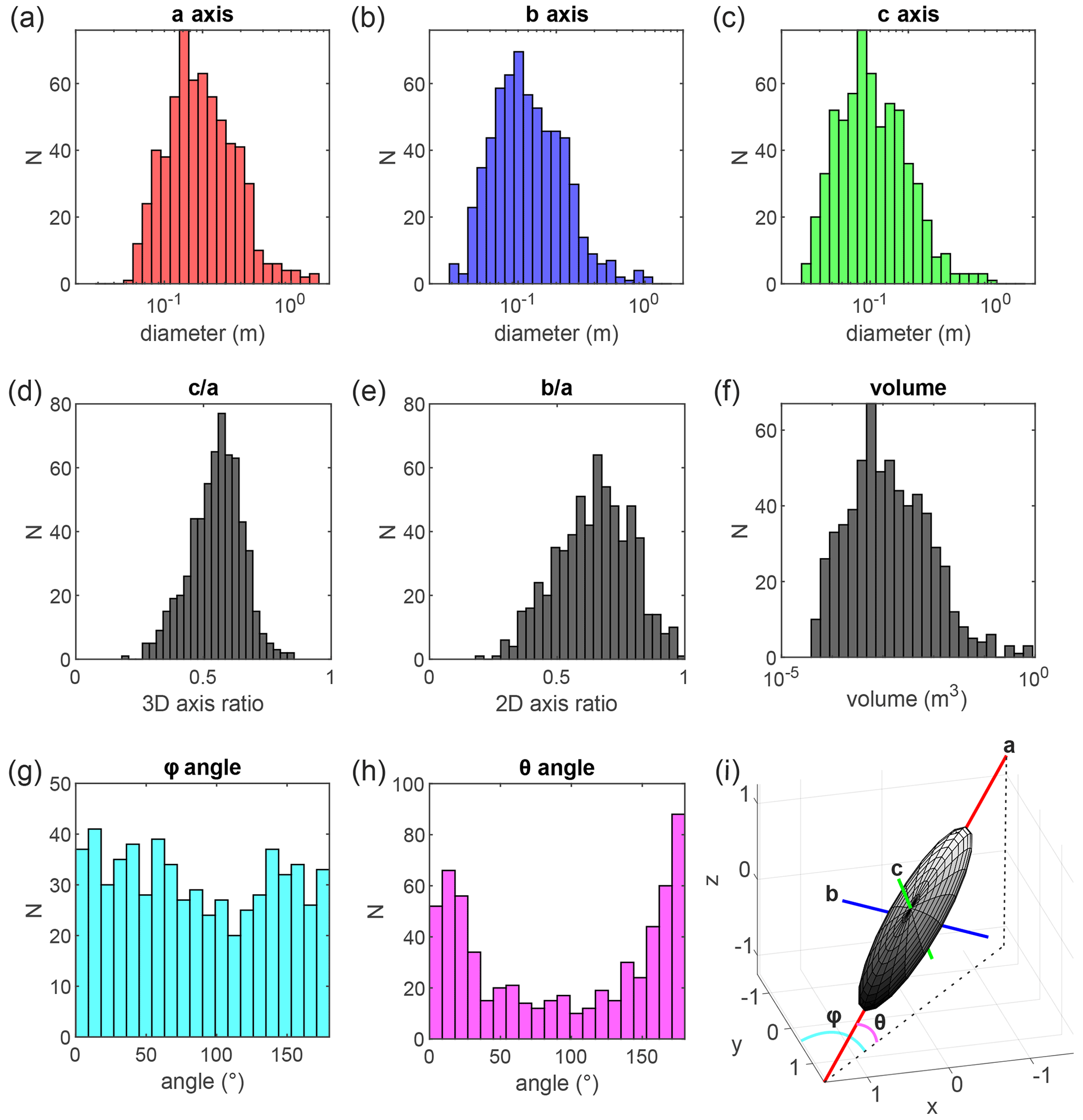
Figure 3 Size, shape and orientation distribution of 630 ellipsoids correctly fitted to the labeled grains. Histogram distribution of the diameters of the ellipsoids along their (a) major a, (b) intermediate b and (c) short c axis. Histogram distribution of the (d) 3D axis ratio ($c/a$), (e) 2D axis ratio ($b/a$) and (f) volume of the ellipsoids. Histogram distribution of the (g) azimuth φ and (h) dip θ angle. (i) Three-dimensional view of an arbitrary ellipsoid and representation of the different metrics used to characterize ellipsoid size, shape and orientation.

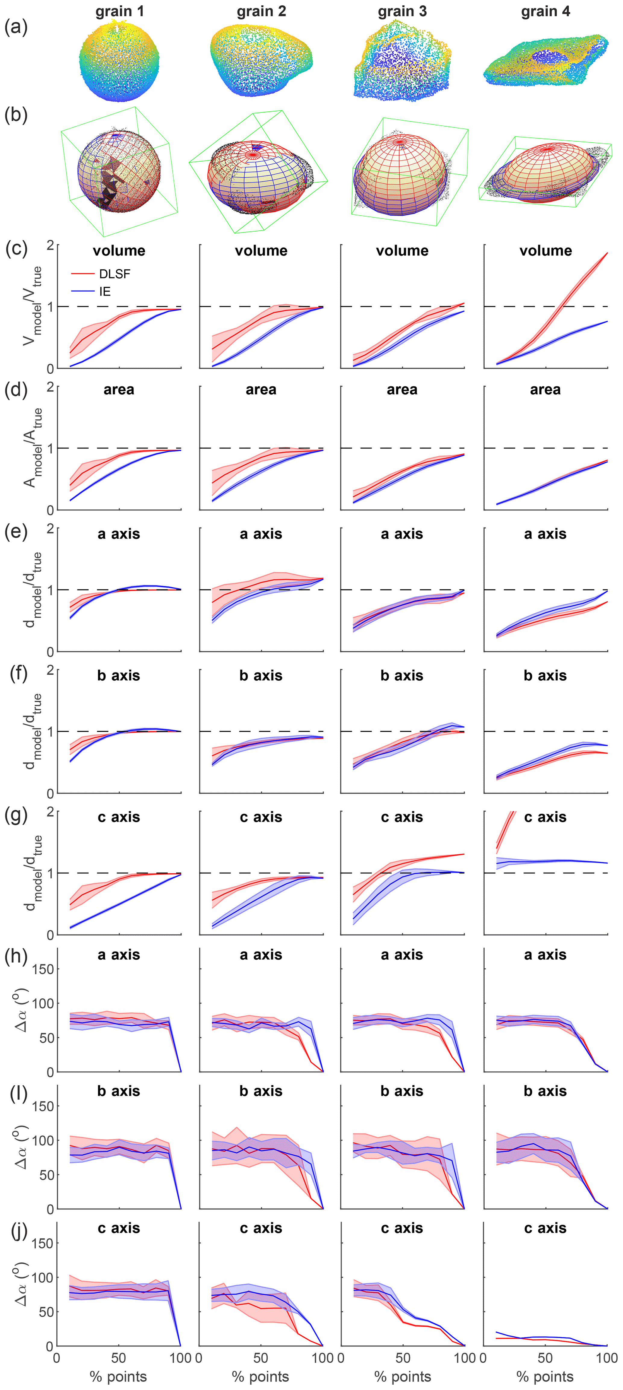
Figure 4 Influence of the grain surface covered by 3D data on the modeled ellipsoidal geometry of a grain. (a) Point clouds of the four tested grains, which consist of grains with increasing angularity and elongation from left (grain 1) to right (grain 4). (b) Resulting bounding box (green) and ellipsoid fit on each grain (black dots), using either the direct least-square fitting algorithm DLSF (red) or the inertia ellipsoid algorithm IE (blue). (c) Volume V and (d) surface area A of the modeled ellipsoids normalized by the volume and area of the convex hull of the point clouds of the entire grains, regarded as true estimates. Length of the modeled (e) a axis, (f) b-axis and (g) c axis normalized by the major, intermediate and minor length of the bounding box around the entire grain. Three-dimensional angle between the 3D vector of the (h) a axis, (i) b axis and (j) c axis with the orientation of the same vector resulting from the ellipsoid fitting the entire grain. In panel (c) to (j), results obtained with the direct last-square fitting approach (DLSF) and the inertia ellipsoid approach (IE) are represented in red and blue, respectively. The error bar, given as a shaded surface around the mean value (solid line), is the standard deviation of the considered metrics obtained by changing 10 times the random seed.

Fitting an ellipsoid to a set of points in 3D is a complex problem that has received attention from different applied mathematics communities, including computer vision, pattern recognition, numerical analysis and statistics. Ellipsoids belong to the family of quadric surfaces that can be defined as

$$\begin{array}{}\text{(1)}& \begin{array}{rl}A{x}^{\mathrm{2}}& +B{y}^{\mathrm{2}}+C{z}^{\mathrm{2}}+\mathrm{2}F\mathrm{yz}+\mathrm{2}G\mathrm{xz}+\mathrm{2}H\mathrm{xy}\\ & +\mathrm{2}Px+\mathrm{2}Qy+\mathrm{2}Rz+D=\mathrm{0},\end{array}\end{array}$$

where A, B, C, F, G, H, P, Q, R and D are the parameters of the quadric surface. Defining $I=A+B+C$ and $J=\mathrm{AB}+\mathrm{BC}+\mathrm{AC}-F^{\mathrm{2}}-G^{\mathrm{2}}-H^{\mathrm{2}}$, it can be shown that Eq. (1) must represent an ellipsoid when $\mathrm{4}J-I^{\mathrm{2}}>\mathrm{0}$ (Li and Griffiths, 2004). This condition is respected when the short radius is at least half the length of the major radius of an ellipsoid. This represents a sufficient condition, but not a necessary one, and ellipsoids can be mathematically defined without respecting $\mathrm{4}J-I^{\mathrm{2}}>\mathrm{0}$. We use an efficient and robust Matlab version (Hunyadi, 2022) of a direct least-square fitting method (Li and Griffiths, 2004), based on the condition that $\mathrm{4}J-I^{\mathrm{2}}>\mathrm{0}$, to describe the geometry of the segmented grains by minimizing the square of the distance between labeled points and the ellipsoidal model. For ellipsoids fitting grains which do not satisfy this condition, the fitting method might still lead to ellipsoids or to other quadric surfaces. Grains suffering from fitting issues or leading to quadric surfaces other than an ellipsoid are filtered out, leaving 630 correctly fit ellipsoids over 657 labeled grains. The resulting ellipsoids, fitted to each labeled grain, appear qualitatively consistent with the shape, size and orientation of the labeled grains (Fig. 2d). Other ellipsoidal fitting algorithms exist, but this direct least-square approach was found to lead to the best solution for the data set we used. In turn, the condition $\mathrm{4}J-I^{\mathrm{2}}>\mathrm{0}$ prevents the occurrence of flat or over-elongated ellipsoids, which could otherwise represent better mathematical solutions despite being, in some cases, physically unlikely.

The second approach considered to characterize the geometry of the grains computes the inertia ellipsoids corresponding to the labeled points of the grains. This is performed first by computing the mean position of the points, second by computing the covariance matrix of the points subtracted from their mean position and third by making an SVD of the covariance matrix normalized by the number of points.

The approach based on the inertia ellipsoid can be considered simpler than the direct least-square fitting method and does not suffer from mathematical constraints of the direct least-square approach. However, as it is not a fitting method, its main drawback is that it is unable to guess the “hidden” geometry of the grains (i.e., by using the curvature of the visible part of the grain), and the obtained inertia ellipsoids will tend to be flatter than the grains. We later compare the two approaches in the Results section. We also compare the obtained ellipsoids to cuboids that are obtained by determining the minimal 3D bounding box for each grain, with at least one side oriented along the horizontal plan. More specifically, the orientation and dimensions (i.e., length, width and height) of the cuboids are compared to the orientation and dimensions of the major, intermediate and short axes of the ellipsoids.

2.5 Geometrical and statistical description of grain size, shape and orientation

Once the grains are fitted by an ellipsoid, it is straightforward to access their geometrical information. For each ellipsoid, we measure the radius (and the diameter, as classically used for grain-size distributions) of the major a, intermediate b and short c axes, the orientation (i.e., azimuth and dip) of these three axes, the volume of the ellipsoid $V=\mathrm{4}/\mathrm{3}\mathit{\pi }abc$, and the approximate surface area A of the ellipsoid using Knud Thomsen's formula $A=\mathrm{4}\mathit{\pi }{\left(\left(a^p{b}^p+a^p{c}^p+b^p{c}^p\right)/\mathrm{3}\right)}^{\mathrm{1}/p}$. Indeed, there is no general formula for estimating A and this formula approximates the ellipsoid area with an error of less than 1.061 % when p=1.6705. We can also compute two different axis ratios, with $c/a$ the 3D axis ratio between the short and major axis and $b/a$ the 2D axis ratio (or elongation ratio) between the intermediate and the major axis. We coin this latter the 2D axis ratio as it generally corresponds to the axis ratio measured from 2D images, by contrast with the 3D axis ratio that is generally not measurable from 2D images (i.e., assuming that the short axis is oriented vertically).

For each grain, we can also compute the distance of each point of the grain, of coordinates (xyz), to its projection on the ellipsoid surface, of coordinates (x_ey_ez_e). The square of this distance, corresponding to the residuals in a least-square sense, characterizes the goodness of the fit through the coefficient of determination:

$$\begin{array}{rl}{R}^{\mathrm{2}}=\mathrm{1}& -\sum \left({\left(x-x_{\mathrm{e}}\right)}^{\mathrm{2}}+{\left(y-y_{\mathrm{e}}\right)}^{\mathrm{2}}+{\left(z-z_{\mathrm{e}}\right)}^{\mathrm{2}}\right)\\ & /\sum \left({\left(x-\overline{x}\right)}^{\mathrm{2}}+{\left(y-\overline{y}\right)}^{\mathrm{2}}+{\left(z-\overline{z}\right)}^{\mathrm{2}}\right),\end{array}$$

with $\overline{x},\overline{y},\overline{z}$, and the mean coordinates of the points. R² provides information on the quality of the mathematical fit itself and on the consistency between the ellipsoidal model and the shape of the grain, which can deviate significantly from an ellipsoidal geometry.

The statistical description of grain geometrical properties of a grain population, such as the classical 1D grain-size distribution (GSD), is then performed based on the geometrical attributes of each individual grain of the considered population (Fig. 3). The range of measured diameters, ∼0.01 to ∼1 m, spans 2 orders of magnitude (Fig. 3a–c), and the 3D ($c/a$) and 2D ($b/a$) axis ratios unsurprisingly vary between 0 and 1 with mean values of 0.55 and 0.65, respectively (Fig. 3d–e). The range of volume of the ellipsoids spans almost 5 orders of magnitude, from 10⁻⁵ to 1 m³ (Fig. 3f). In addition to this classic description, G3Point also provides information on the 3D organization of the grains. Here, the orientation distribution of the grains along this active alluvial bed shows that there is no preferential orientation of grains due to the river flow, as they appear to follow a mostly uniform distribution of the azimuth φ (Fig. 3g), and, as testified by their dip angle θ, that most grains are lying in a sub-horizontal position with $\mathrm{0}<\mathit{\theta }<\mathrm{30}$ or $\mathrm{150}<\mathit{\theta }<\mathrm{180}{}^{\circ }$ (Fig. 3h).

3 Results: method validation and application to lab or natural environments

In addition to its robustness and efficiency, an algorithm dedicated to extract granulometric information from point clouds must be able to manage various sources of data, including SfM and lidar. In the following, we therefore test the newly developed algorithm against “ground truth” data sets of grain size, obtained in the lab or natural environments. For each data set, we compare the distribution obtained with G3Point to the grain-size distribution measured by hand. It is important to highlight that the grain sampling approach of G3Point belongs to the family of areal or area-by-number approaches. We first start by assessing the pros and cons of the different grain fitting approaches by applying them to individual grains of various shapes.

3.1 The influence of grain shape and surface cover on the resulting ellipsoid size and orientation

Two strategies are adopted to describe the geometry of a grain with an ellipsoidal model: fitting an ellipsoid by a direct least-square fitting approach (DLSF) or determining its ellipsoid of inertia (IE). We here test the influence of using these two strategies on the quality of the resulting geometrical models, for individual grains, considering a variable surface covered by the point cloud (Fig. 4).

Indeed, in natural environments, grains have a significant proportion of their surface that is not topographically described, as it is hidden under the grain itself, by other grains or features (e.g., vegetation, water), or due to a lack of visibility with respect to the sensor (e.g., lidar station). The tested grains consist of a spherical ball (grain 1), a low-angularity grain (grain 2), an angular grain (grain 3), and an angular, flattish and elongated grain (grain 4). The point clouds representing the surface of these four grains were obtained by SfM using Agisoft Metashape. Each grain was put on a 1 cm radius plastic plate attached to the top of a tripod and about 50 pictures were acquired all around the grain. For each of these point clouds, we generated ellipsoidal models considering only a prescribed percentage of their surface covered by the point cloud, from 10 % to 100 %. Practically, surface cover is varied by first choosing a random seed among the points of the point cloud and then sampling a number of nearest neighbors leading to the sought surface cover of the grain. Ellipsoidal modeling by DLSF and IE is then applied only to this sampled part of the total point cloud. The modeled ellipsoidal volume V_model and surface area A_model are then compared to the volume V_true and surface area A_true of the convex hull of the point cloud. The modeled diameters d_model of the three axes are compared to the dimensions d_true of the bounding box of the point cloud. Last, the 3D angle Δα, between the modeled orientation of the ellipsoid axes and axes of the “true” ellipsoid obtained by considering the entire grain, is computed. For each surface cover, 10 samples are tested, leading to 10 models obtained by the DLSF and IE approaches, allowing us to define a mean value and a standard deviation for each metric.

For the two low angular grains (grains 1 and 2), metrics obtained with DLSF or IE are consistent with the true geometry of the grain even for relatively low surface cover, down to 20 %–30 %. DLSF gives significantly better results than IE, in particular for a surface cover between 20 % and 80 %, which likely represents a common range for most labeled grains. Thanks to grain curvature, the DLSF fitting algorithm also converges towards value for V, A and d which are close to the true values. For the orientation, both approaches are unable to converge towards the true one for the spherical grain (i.e., grain 1), which is not surprising as the orientation of a sphere is not defined. For grain 2, both approaches converge slowly towards the true orientation for a surface cover greater than 50 %–75 %.

For the angular grain (grain 3), the DLSF and IE approaches give similar results. The dimensions are well captured for a surface cover greater than 60 %–70 %. The orientation, in particular of the c axis, converges more rapidly than for low-angularity or spherical grains. For the angular, elongated and flattish grain (grain 4), the IE approach gives better results than the DLSF for the length of the c axis and the volume, while other metrics are relatively similar. Indeed, the algorithm of the DLSF imposes some constraints on the minimum size of the c axis compared to the a axis, which makes it unable to properly capture the 3D dimensions of flattish grains.

These results show that the dimensions of spherical or low-angularity grains are well captured by the IE and DLSF approaches, with this latter giving good results even for a surface cover lower than 50 %, while their orientation is poorly captured for a surface cover lower than ∼75 %. On the other hand, grains that clearly depart from the spherical model, in particular due to their high angularity, need a greater surface cover, around 60 %–70 %, to be properly captured for their dimensions by ellipsoidal models, while their orientations converge more rapidly towards their true value. Flattish grains are better modeled by the IE approach, as the DLSF leads to a large value of the c axis. Last, we note that the orientation of the c axis is generally better captured than the one of the a and b axis, which suggests that the azimuthal orientation of grains is less well resolved than their inclination (assuming that the c axis of grains is sub-vertical).

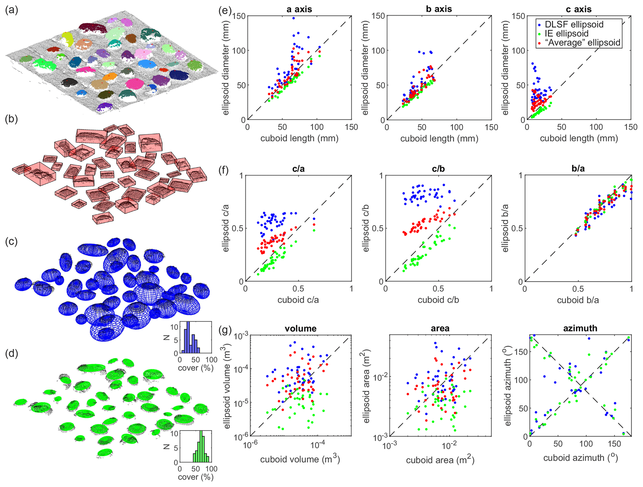
Figure 5 Results from the lab experiment considering 39 pebbles on a flat surface. (a) Point cloud (gray dots) of the experiment overlaid by the label (color) of each identified grain and their summit node (red dot). The resulting (b) cuboid (red) and ellipsoids obtained with (c) a direct least square (DLSF, blue) and (d) the inertia ellipsoid (IR, green) approaches. Diameters measured along the (e) a axis (left), b axis (center) and c axis (right) using the direct least square (DLSF, blue dots) and the inertia ellipsoid (IE, green dots) approaches for the 39 grains as a function of the cuboid lengths (see Fig. S4). The red dots show the dimensions of the average ellipsoid between the IE and DLSF ellipsoids. (f) Axis ratios of the ellipsoids as a function of the axis ratios of the cuboids. (g) Volume, area and azimuthal angle of the a axis (0–180^∘) of the ellipsoids as a function of the azimuthal angle of the cuboids. The black dashed lines show the 1:1 line on all the panels.

3.2 Lab experiment: the test of the pebbles on a flat surface

Here, we apply G3Point to a lab experiment, consisting of 39 black pebbles, bought in a hardware store, lying in a horizontal position over a planar surface of 0.5×0.5 m (Fig. 5a). This lab experiment was photographed using a Nikon D3500 in a 4000×6000 pixel format with about 50 pictures, taken with different angles, to generate a 3D point cloud by SfM. Data were processed with Agisoft Metashape and the resulting point cloud, made of $\sim \mathrm{2}\times {\mathrm{10}}^{\mathrm{5}}$ points, has a native point density of ∼1 point per mm⁻¹. To segment grains, and only grains, the planar surface is removed from the point cloud by removing all the points below a threshold elevation over the vertical coordinate. G3Point is then applied to this point cloud using the couple of parameters k=100 and C_F=0.8, after a trial-and-error series of tests. Indeed, the 39 pebbles are perfectly detected and labeled as individual grains. Each grain is then described by a cuboid (Fig. 5b) and ellipsoidal models using the direct least-square fitting method (DLSF) (Fig. 5c), as previously done, and the inertia ellipsoid (IE) approach (Fig. 5d). We force the vertical dimension of the cuboids to start at the elevation of the planar surface for their lower face, to correctly capture the height of the grains. As the grains are lying flat, the length and the width of the cuboids correspond to the long and intermediate axes of the grains, respectively. The major a, intermediate b and short c axes of the modeled ellipsoids are then compared to the true diameters of the pebbles, which are assumed to be characterized by the length, width and height of the cuboids, respectively. We emphasize here that most of the pebbles used for this test are strongly elongated ($b/a\sim \mathrm{0.5}$) and flat ($c/a\sim \mathrm{0.25}$), which can represent real challenges for most ellipsoidal fitting algorithms. This test should therefore be regarded as an end-member scenario, testing the ability of the approach to properly describe the geometry of grains using ellipsoidal models.

Despite this, the obtained diameters for the a, b and c axes are roughly consistent between the three approaches (Fig. 5e), even if the diameters obtained with the DLSF and IE approaches are systematically higher or lower, respectively, than the cuboid dimensions. The ratios between the ellipsoid diameters and the cuboid lengths for the a and b axis range between 0.8 and 1 for the IE and between 0.8 and 2 for the DLSF (see Fig. S4 in the Supplement). For the c axis, the consistency is less good and the ratio range between 0.4–0.9 and 1.1–9 for the IE and DLSF approaches, respectively. These results reflect the pros and cons of each approach: the DLSF approach leads to larger than expected ellipsoids, due to the geometrical constraint of the fitting algorithm for the c axis, while the IE approach leads to smaller than expected ellipsoids, as only the upper face of the grains is accounted for. This is well illustrated by the difference in the resulting 3D ($c/a$) and 2D ($b/a$) axis ratio. If the 2D axis ratio is relatively consistent between the three approaches (Fig. 5f), the 3D axis ratio of the DLSF ellipsoids (0.4–0.65) is significantly higher than the one of the cuboids (0.1–0.4), except for one grain. By contrast, the 3D axis ratio of the IE ellipsoids is always lower than the one of the cuboids. These discrepancies also lead to a larger or lower volume and area for the DLSF or IE ellipsoids, respectively, compared to the cuboid volume and area (Fig. 5g). We note that the consistency of the DLSF ellipsoids with the cuboids is greatly improved when increasing the 3D axis ratio (i.e., when considering more spherical grains), which limits the role of the geometrical constrain on the quality of the fit ellipsoid. Last, the horizontal orientation of the DLSF or IE ellipsoids, given by the azimuthal angle of the a axis, is relatively consistent with the orientation of the cuboids (Fig. 5g).

Despite a good first-order accuracy of the considered ellipsoidal models to represent the 3D dimensions of grains, none of these approaches is deemed systematically suitable by itself. The consistency of the ellipsoidal models with the true geometry of the grains depends on the considered geometrical model, on the surface coverage of the grain by the point cloud and on the shape of the grain itself (Fig. 4). In the following, instead of relying on a single ellipsoidal model, we rather assess the geometry and dimensions of grains by using both the DLSF and IE ellipsoidal models. Indeed, considering the size (or size distribution) obtained with the DLSF and IE ellipsoidal models offers an upper and lower bound on the true size (or size distribution) of the grain (or grain population). We also provide a mean size (or size distribution) obtained with these two ellipsoidal models to offer an approximate solution to the true size of the grain (or grain population).

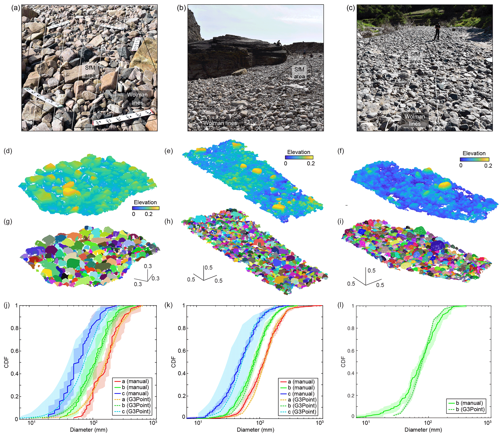
Figure 6 Field pictures (a–c), initial point clouds colored coded in elevation and segmented point clouds (d–i), and grain-size distributions (j–l) from (a) Site 1 and (b) Site 2 of the Pointe du Château Renard and (c) the Hérault River. Distributions of the a (red), b (green) and c (blue) axis result from Wolman counts (dark colors) and G3Point (light color dash lines). Shaded envelopes correspond to uncertainties defined by bootstrap approach for Wolman counts and by the envelope defined by the two fitting methods for G3Point (see text for details). Locations of the Wolman lines (white) and SfM covers (black polygons) are indicated in the pictures.

3.3 Field experiments with SfM 3D point clouds

The second experiment consists of pebbles from three natural field sites in France: the beach of Pointe du Château Renard (Brittany) with coarse and angular grains at Site 1 and smaller rounded grains at Site 2 (Fig. 6a–b) and the Hérault River near Saint-André-de-Majencoules (Cévennes) with rounded, fluvially transported pebbles (Fig. 6c). At each site, we sampled the grain-size distribution by the Wolman grid-by-number method (Wolman, 1954). At Site 1 of Pointe du Château Renard, we defined a grid of about 2.5×3 m with nodes every 0.3 m, we measured the three axes of each grain lying under a node, and a total of 76 grains were measured. At Site 2, we stretched two parallel decameters and two operators walked along these lines, picked the two grains lying under each of their hands (random selection) about every meter and measured the three axes of the grains. In total, 529 grains were measured. For the Hérault River, we defined a grid of 2.5×13 m with nodes every 0.4 m and we measured the intermediate axis of 197 grains. The others diameters were not measured due to time constraints. Measurements were performed with a calliper and rounded toward the nearest millimeter or with a decameter and rounded toward the nearest 5 mm, for small or large grains, respectively. Only grains larger than 4 mm were measured.

In addition to operator errors, related to the measurement itself and to the choice of the diameter to measure, the resulting distribution is associated with uncertainties related to the size of the sample. We used a bootstrap approach with replacement to evaluate the confidence interval of each distribution (Rice and Church, 1996; Bunte and Abt, 2001; Green, 2003). For each sample, we randomly sampled 10 000 replicates of the distribution, and the scatter defines the confidence interval. The pebbles at Site 1 of the beach of Pointe du Château Renard have a median a axis of 170±48 mm, a median b axis of 110±40 mm and a median c axis of 60±20 mm (Fig. 6a, Table S1 in the Supplement). At Site 2, the pebbles have a median a axis of 117±15 mm, a median b axis of 80±9 mm and a median c axis of 50±6 mm (Fig. 6b, Table S1). The fluvial pebbles along the Hérault River are smaller, with a median b axis of 75±18 mm (Fig. 6c, Table S1).

Table 1 Statistics of the grain-size distributions for the three sites surveyed by SfM. The six coefficients (k, CF, α, β, φ_flat, A_thres) are the parameters required for G3Point (see text for details).

At Château Renard, we used a Nikon D3500 in a 4000×6000 pixel format, and for the Hérault River, we used a Nikon D7500 in a 4176×2784 pixel format. At each site, we took about 100 pictures covering a few square meters to build a 3D point cloud by SfM. Data were processed with Agisoft Metashape and the resulting point clouds have a native point density of ∼1 point per mm⁻¹. We subsampled the point clouds with CloudCompare to ∼ one point per 2 to 3 mm to reduce calculation duration. G3Point is then applied to the resulting point clouds with parameters defined after a trial-and-error series of tests so that the segmentation of the grains is visually satisfying (Table 1, Fig. 6).

A large number of grains are detected (428, 1077 and 678 for Château Renard Site 1, Site 2 and the Hérault River, respectively, Table 1). Yet, to compare the distributions obtained by G3Point to the distributions obtained by Wolman counts in the field, we must perform virtual Wolman samplings on the fitted grains. We apply a virtual grid to the 3D point cloud and automatically extract the three axes of the grains lying under the nodes, with grid spacing defined as half the maximum b axis (this roughly corresponds to the D90). Because we can easily resample the point cloud, we repeat this operation 25 times and define the grain-size distribution as the average of these 25 samples, for each fitting method. The DLSF and IE distributions are used as the confidence interval of the average distribution (see Method section). We now have 77, 332 and 183 grains for Château Renard Site 1, Site 2 and the Hérault River, respectively (Table 1). The confidence intervals of the a and b axis are up to ±14 %, but we observe intervals close to ±50 % for the c axis due to the assumptions made by the fitting methods for the c axis (Table S1, and see the Method section for details).

Figure 7 Comparison of the key percentiles (10th, 16th, 25th, 50th, 75th, 84th, 90th) obtained by manual counts and by G3Point at the three study sites and for the three diameters. Distributions from G3Point are derived from the virtual Wolman sampling and uncertainties correspond to the envelopes defined by the DLSF and IE models. For manual counts, uncertainties are derived from a bootstrap approach with replacements. The dash lines indicate a 1:1 ratio (points under/above the line indicate that G3point under/overestimates the percentile with respect to field measurements).

To better compare the two approaches, we compare the key percentiles (10th, 16th, 25th, 50th, 75th, 84th, 90th) of the grain-size distributions obtained by manual counts and by virtual Wolman on the segmented point cloud (Fig. 7). For each diameter at each study site, points align along a 1:1 line in a quantile–quantile diagram, indicating that the average distributions obtained with G3Point are similar to the ones obtained by manual counts (Fig. 7). In particular, the 50th percentiles (i.e., the D50s of the distributions) fall very close on the 1:1 line of the Q–Q plots, implying that G3Point leads to similar median diameters for any grain axis. As observed with the previous examples, the DLSF and the IE approaches perform similarly well on the a and b axis but they tend to overestimate and underestimate the c axis, respectively (Fig. S5). Other diameters are within uncertainties but must be considered with more care (Fig. 7, Table S1). In fact, at Site 1, G3Point tends to underestimates the smallest percentiles of the distributions and to overestimate the coarsest ones (Fig. 7a–c). Yet, this discrepancy is limited and always within the error bars of manual counts. For example, for the a axis, the D90 measured on the field is 304±135 mm, while it is 334±46 mm with G3Point (overestimation by ∼10 %, Fig. 7a). We observe the opposite trend at Site 2 and for the Hérault River, with an overestimation of the smallest percentiles and an overestimation of the coarsest ones (Fig. 7d–f). Here again, this trend is quite limited as, for example, the D10 of the b axis at Site 2 is 38±6 mm from manual counts and 43±3 mm with G3Point (overestimation of ∼13 %). The algorithm is unable to recover small grains because they are described by a limited number of points. As a consequence, the worst performance of G3Point is observed for the small percentiles of the c axis. For example, at Site 2, the D10 of the c axis is overestimated by ∼35 % (Fig. 7f, Table S1).

This second experiment based on natural grains thus confirms that G3Point is efficient at recovering Wolman-like grain-size distributions for pebble and cobble populations in different environments and for various grain angularity, with a limited temporal cost in the field and in the lab.

4 Discussions

4.1 Practical considerations for using G3Point

As already demonstrated, G3Point is designed to perform semi-automatic 3D granulometric measurements on point clouds over surface area 1: 100 m² (hereinafter referred to the patch scale) with a typical point density of $\sim \mathrm{0.1}-\mathrm{1}$ cm per point and a total number of points around 10⁶. The point density should be high enough so that each grain is described by at least several dozen points. This scale enables us (1) to perform efficient and fast measurements (i.e., several seconds), (2) to visually check the quality of the resulting segmentation of the grains, and (3), if needed, to compare the resulting grain-size distribution with the one obtained with manual counting. We therefore suggest using G3Point mostly for patch-scale studies. In terms of computational time, there is a tradeoff between the total surface area and point density. G3Point can also perform grain size, shape and orientation analysis over larger study areas (>100 m²). In this case, the best practice consists either (1) in decreasing point density and in turn losing the ability to detect smaller grains or (2) in segmenting the initial point cloud into several sub-point clouds, at the patch-scale and with the initial point density, which can then be successively processed by G3Point. We generally recommend validating the results against some field measurements (e.g., grain-size distribution obtained by a Wolman count), at least on some parts of the studied area. When no classical grain-size data are available, we recommend carefully checking the results of the grain segmentation phase and testing its sensitivity to the different parameters of G3Point. For instance, this could be the case for the measurement of grain size and shape on other planetary bodies (Szabo et al., 2015; Lauretta et al., 2019; Burke et al., 2021) or in inaccessible and remote areas. The outcomes of G3Point are tightly linked to the choice of the local neighborhood scale through the parameter k. This parameter should therefore be taken as small as possible to enable the segmentation of small grains but not too small to prevent the over-segmentation of large grains due to local topographic minima associated with surface roughness or noise. Suitable values of k are generally determined by a trial-and-error series of tests (Fig. S1).

4.2 SfM- or lidar-derived point clouds?

As demonstrated in this paper, G3Point can be applied to point clouds obtained with a terrestrial lidar or by SfM. Point clouds obtained with terrestrial lidar data provide better accuracy than SfM but can be associated with varying point density, while the ones obtained by SfM provide uniform point density but can lead to some inaccuracies. In particular, point clouds obtained with SfM were observed to generate smooth or inaccurate topographic transitions between grains, as these correspond to “shadow” areas difficult to capture with pictures. This might be related to the quality of the photos (lighting, blurring, resolution), as with any SfM study. These smooth transitions are not too problematic for G3Point, as it is based on the steepest slope, but they prevent efficiently using a criterion based on topographic curvature to segment grains or to correct the segmentation obtained with G3Point. In that case, we recommend removing points located at local topographic minima to ease segmentation (this is an option provide by G3point). For lidar data, the issue of spatially varying point density can lead to a non-optimal set of parameters, in particular k, the number of nearest neighbors considered, over the entire surface of the considered point cloud. In this case, we recommend working on sub-point clouds of rather homogeneous spatial point density. The use of point clouds obtained with only one station does not represent an issue for the watershed segmentation of G3Point (Fig. 2), even if it limits the number of data points per grain and their spatial distribution along the surface of the grains, which is not optimal for shape fitting algorithms.

4.3 Comparison of G3Point with previous methods

In terms of total working time, using G3Point over a surface area of about 1–100 m² captured by SfM involves collecting field pictures (∼5–10 min), processing the pictures by SfM to obtain a point cloud (10 min to several hours) and running G3Point several times to find a good parametrization (∼10 min). Interestingly, G3Point itself is not the limiting factor, as field data acquisition (i.e., pictures or lidar data) and data processing (i.e., SfM) appear to be more time-consuming. The total working time is roughly equivalent to a typical manual pebble count, which takes about 60 min to measure the three axes of 100 grains. However, data sampling for G3Point is not destructive; it can be done by a single operator, and G3Point will result in the measurement of a much larger number of grains for the same sample extension (>10² grains) including their size, location and orientation in 3D. It offers a real benefit in terms of representativeness and opens new avenues to quantitatively characterize populations of grains (e.g., not only their size distribution), based on the geometry on their upper surface. Moreover, because point cloud data acquisition in the field is fast, large areas or multiple locations along a fluvial system can be documented in a limited amount of time. In addition, pictures for SfM can be acquired with drones so that remote locations or very coarse-grained environments can be safely characterized. Together with the large number of grains being considered, G3Point represents a real improvement in terms of spatial representativeness with respect to Wolman or photographic approaches which are usually limited to a few square meters and a few hundreds of grains (Bunte and Abt, 2001). Last, while most methods based on 3D data use texture or any other morphological index to estimate the grain sizes (Vazquez-Tarrio et al., 2017; Woodget et al., 2018; Chardon et al., 2020), G3Point works directly on the grains and does not require a calibration phase. Once again, this limits bias and time spent in the field and allows remote areas to be characterized. G3Point shares some common objectives with the automatic method developed by Walicka and Pfeifer (2022), which directly segments grains from 3D point clouds. It uses a random forest algorithm to classify grains and then a DBSCAN algorithm to segment each grain individually. Compared to Chen et al. (2020), who developed a deep learning approach to segment grains based on 3D point clouds, G3Point does not rely on the a priori training of a neural network on thousands or more grains, which can be highly time-consuming. Yet, G3Point could represent a good alternative to train deep learning algorithms, as it can provide thousands of grains in a few minutes that otherwise take weeks of work when manually labeled.

4.4 In situ results on the granulometric conversion factors

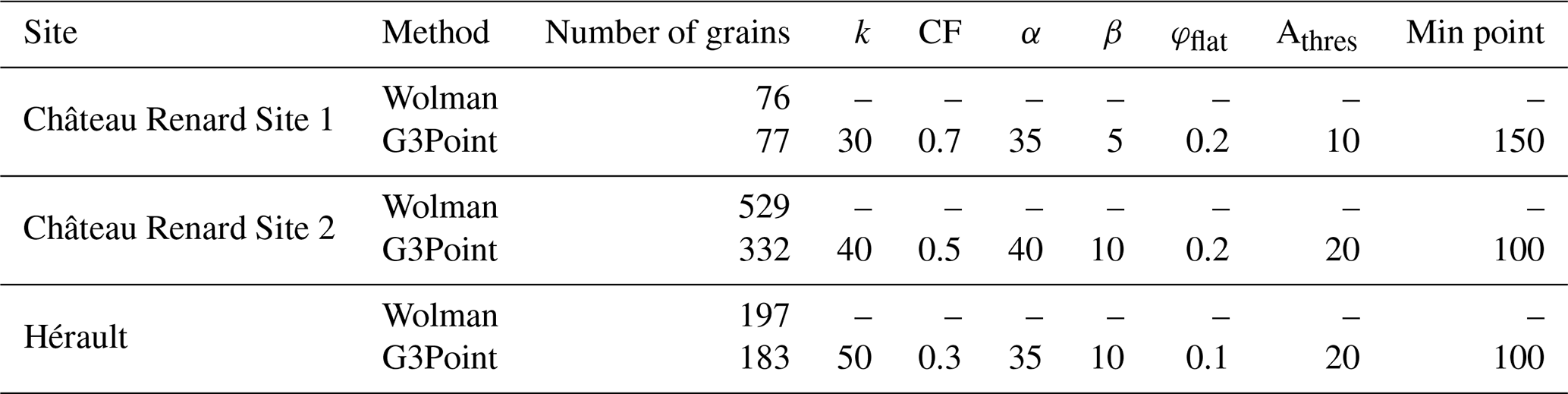
Because G3Point samples virtually all the grains at the surface, it belongs to the family of areal or area-by-number grain sampling approaches. To compare this distribution to the Wolman field counts, it must be converted to a grid-by-number distribution, which is considered equivalent to a volumetric grain-size distribution. Conversion factors have been proposed to convert grain-size data acquired with one approach to another one, based on geometrical arguments (Kellerhals and Bray, 1971; Church et al., 1987; Diplas and Fripp, 1992). For example, converting an area-by-number (or areal) distribution to a grid-by-number (or volumetric; e.g., Wolman) distribution requires multiplying the frequency of all the particle classes by the factor D². However, this exponent of 2 is theoretically valid only for spherical sediments with the same density and without porosity. The use of such a conversion factor thus requires a calibration phase and should, in any case, only be regarded as an approximate conversion method (Bunte and Abt, 2001).

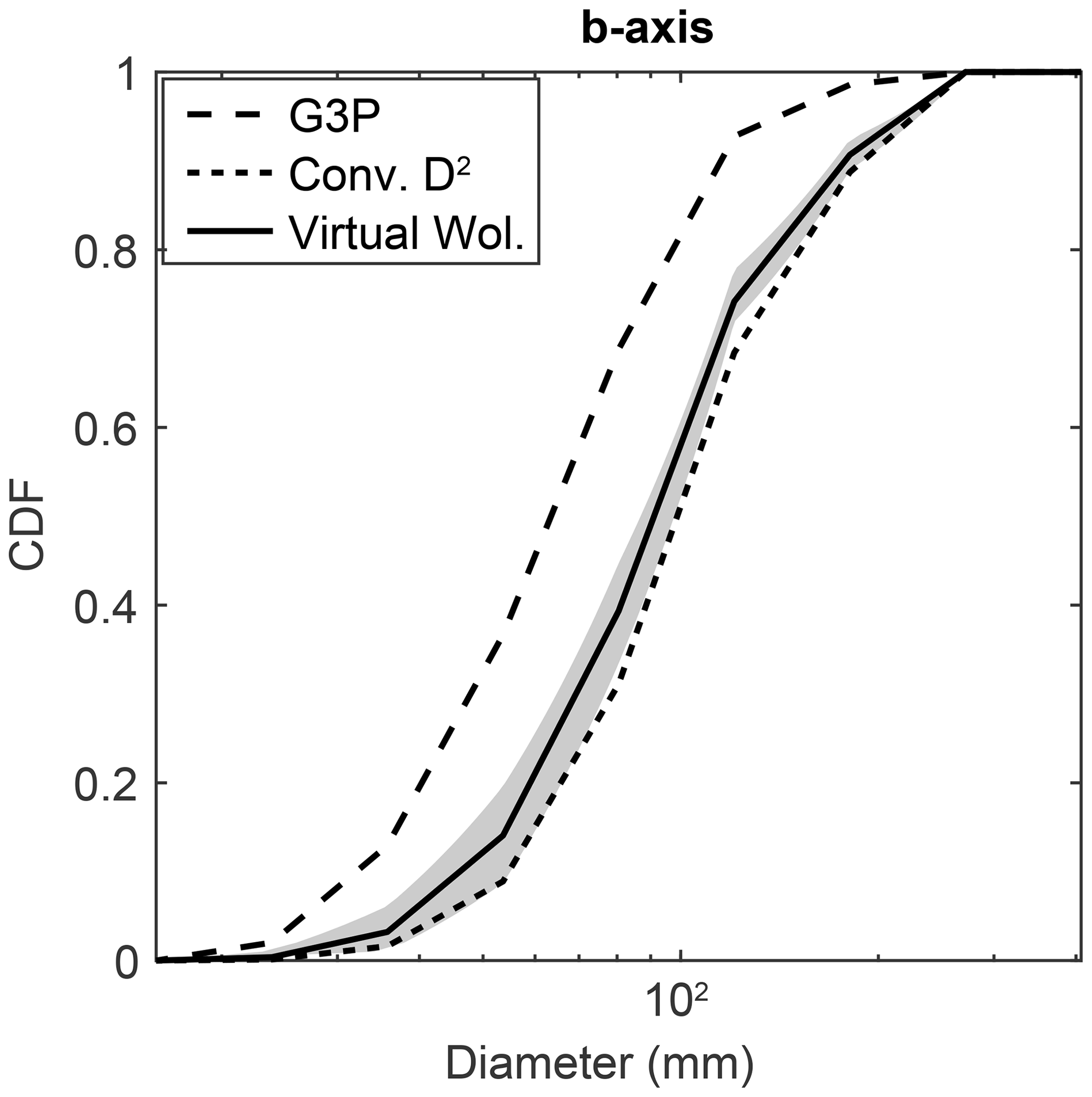
Figure 8 Illustration of conversion from a G3Point grain-size distribution to a Wolman-like distribution. Data are from Site 2 of Château Renard. The initial G3point distribution is an area-by-number one (large dashed line) that can be converted to a grid-by-number (e.g., Wolman) one with a conversion factor of 2 (small dashed line). Alternatively, a virtual Wolman count can be performed directly on the segmented and fitted grains (black line). The shaded envelope indicates the variability observed with 50 realizations.

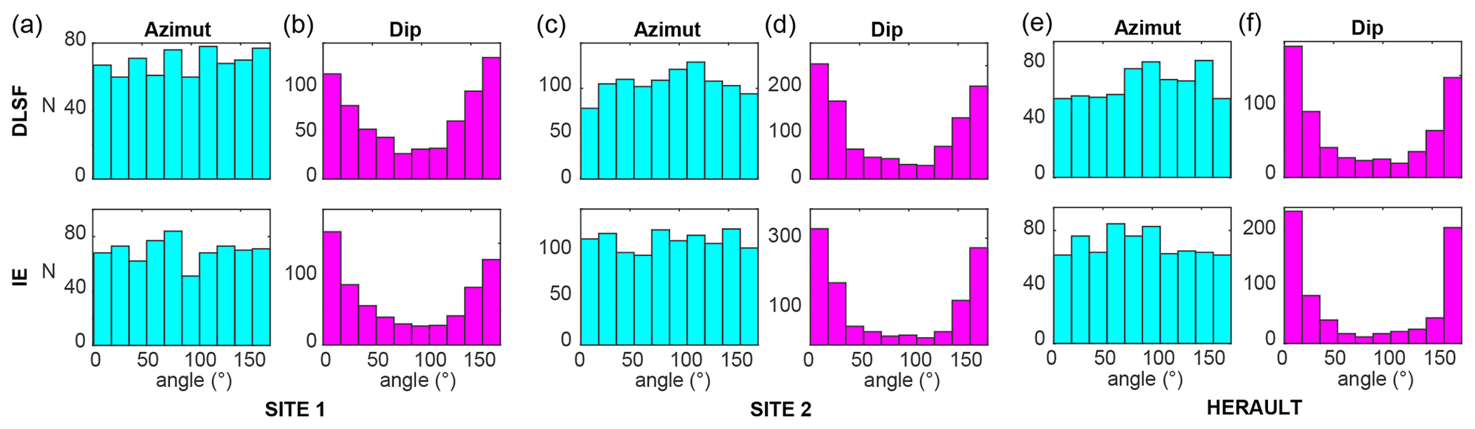
Figure 9 Azimuth and dip angles of the grains fitted to the two approaches (DLSF and IE) at (a–b) Site 1, (c–d) Site 2 and (e–f) the Hérault River. N is the number of grains of a given angle in degree.

With our new approach, we work on 3D point clouds covering large areas, and a large number of grains can be identified. Therefore, instead of converting from an area-by-number to a grid-by-number distribution, we can apply a virtual grid over the point cloud and perform a Wolman count on the fitted grains. To account for the spatial variability of the grains, we repeat this operation 25 times to define an uncertainty envelope and use the average distribution as the grain-size distribution of the sample. For our field examples, we observe that the geometrical conversion is always coarser than the virtual Wolman distribution, yet within uncertainties (Figs. 8, S6, S7, S8). The only exception is for the c axis of the grains with the IE fit. Because this fit leads to very flat ellipsoids, the geometrical conversion factor largely overestimates the size of the grains (Figs. S6, S7, S8). In agreement with previous work (Graham et al., 2010), this suggests that the geometrical factors are a correct approximation that tend to maximize the size of the grains, so that Wolman counts should be favored when possible. We emphasize that the field examples presented above were acquired in order to test our approach and the extent of the point clouds are thus similar to the extent of the Wolman counts performed in the field. Therefore, we sampled approximately the same number of grains in the field and virtually (Table 1). Yet, G3Point is designed to operate on larger point clouds so that a few hundreds of grains will be sampled with the virtual Wolman sampling, allowing for an even more accurate description of the grain-size distribution from point clouds.

4.5 Opportunities to explore and measure uncharted metrics: grain 3D orientation

Here, we briefly present some results on the orientation of grains that we obtain with G3Point. The idea is not to dedicate a detailed study of this metric but to illustrate the ability of G3Point to automatically measure it with no additional efforts. This represents a real benefit of G3Point as most field or picture measurements of grain orientation are either cumbersome or approximate (e.g., using qualitative classification), with the exception of the azimuth angle that can be accessed with approaches based on 2D pictures (e.g., Purinton and Bookhagen, 2019).

The azimuth and dip angles of a grain may give some information about the flow that transported and deposited a population of grains. G3Point offers a very simple way to access the orientation of a large population of grains as the azimuth and dip angles can easily be determined from the fit ellipsoids (Fig. 3). On average, the two fitting methods are efficient at recovering orientation, but they do not lead to the exact same results (Fig. 5g). Therefore, if grain orientation is a key element of a study, preliminary tests may be useful to determine the best-fitting approach in terms of orientation (which may depend for example on the geometry of studied grains). Here, we show the results of both approaches to illustrate their similarity and differences. Azimuth is given with respect to the y axis defined as parallel to the main water flow. At Site 1, the grains show no preferential azimuth (Fig. 9a), and most grains rest flat on the beach, with a dip angle smaller than to 30^∘ or larger than 150^∘ (Fig. 9b). However, 40 % to 50 % of the grains exhibit a dip angle between 30 and 150^∘. We propose that their orientation results from their fall from the nearby cliffs rather than from transport by the sea. At Site 2, a slightly preferential orientation can be inferred from the DLSF fit, with more grains showing an angle with the main flow than grains aligned with the flow (Fig. 9c). Here again, most grains rest flat and 30 %–40 % of them exhibit a dip angle comprised between 30 and 150^∘ (Fig. 9d). We propose that this is due to a stronger control of the sea on this site with respect to Site 1. Along the Hérault River, grains tend to orient themselves perpendicular to the main flow (Fig. 9e) and to rest flat, with 27 %–38 % of them with a dip angle comprised between 30 and 150^∘ (Fig. 9f).

5 Conclusion

The G3Point algorithm presented here makes progress on the issue of grain segmentation and shape analysis from 3D point cloud data. G3Point represents a methodological alternative to previous granulometric approaches, including hand measurements or 2D image analysis. Its main advantages are (1) its computational efficiency and speed that rely on the use of a state-of-the-art watershed algorithm (e.g., Braun and Willett, 2013) to segment grains, (2) its scale-free approach which enables the segmentation of grains with a large range of sizes above the neighborhood scale (i.e., typically a few centimeters), (3) its 3D nature which enables the calculation of metrics (e.g., sphericity, orientation) which are seldom obtained in the field, and (4) its ability to perform a large number of measurements, which favors a good representativeness of the results.

The G3Point algorithm was able to properly describe the size and orientation of grains in a lab experiment. It was also qualitatively successful compared to hand measurements (e.g., Wolman count) in segmenting and quantitatively capturing the size distribution of hundreds to thousands of grains in fluvial and coastal environments. The modeling of grain geometry was performed using ellipsoidal models obtained either with a direct least-square fitting approach or by taking the inertia ellipsoid. Both ellipsoid models accurately infer the major and intermediate axes, but the inertia ellipsoids and the direct least-square ellipsoids tend to underestimate or overestimate the minor axis, respectively. This in turn impacts the ability of G3Point to infer the volume and surface area of grains. For the minor axis, the mean value of the inertia and direct least-square ellipsoids provides estimates that are consistent with hand measurements. Other geometrical models were tested, including bounding boxes. We acknowledge that future work could focus on providing better geometrical models or a better fitting approach to describe the geometry of grains. Alternatively, future efforts could investigate the surface geometry of segmented grains by G3Point, without relying on fitted geometrical models (e.g., ellipsoidal model) but by exploring the topology of the segmented point clouds. An inherent limit remains that, in natural environments, only a fraction of the grain surface is visible and can be topographically described using lidar or SfM.

Fascinating and first-order issues remain for understanding the shape and size of grains and interpreting them in terms of abrasion and fragmentation processes (Domokos et al., 2014, 2015, 2020; Novák-Szabó et al., 2018). This is pivotal for better exploiting the unique geological archives contained in the size, shape and orientation of grains found in natural systems on Earth and other planetary bodies (e.g., Szabo et al., 2015). G3Point, by filling a methodological gap, could foster the development of a more systematic characterization of grain shape in natural environments and lead to a better understanding of the physics of geomorphological processes and of their past dynamics.

Appendix A

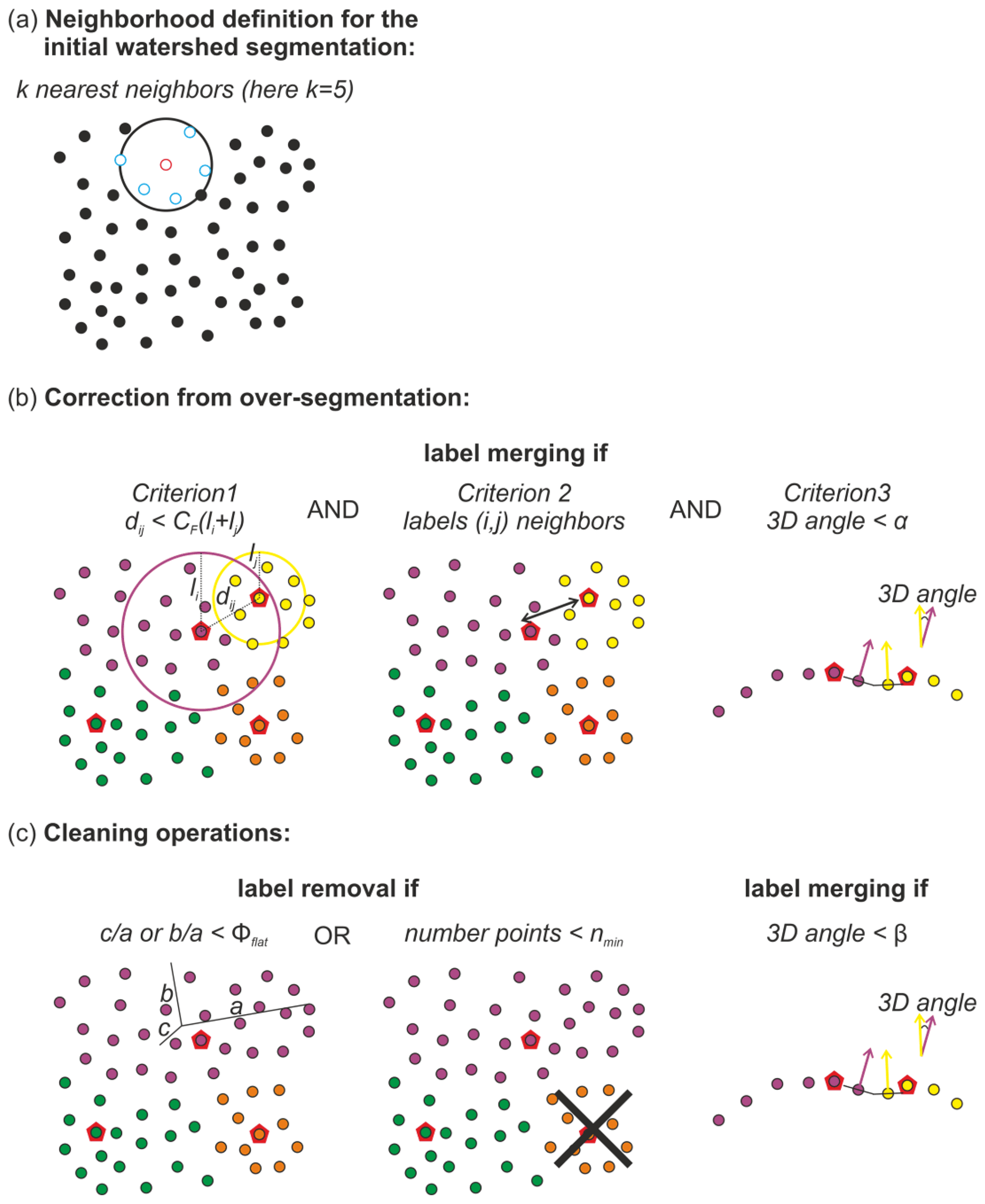
Figure A1 Schematic schemes illustrating the different parameters of G3Point used during (a) the initial watershed segmentation (see Sect 2.1), (b) the correction of the initial segmentation from over-segmentation by grain merging (see Sect. 2.2) and (c) the cleaning of the segmentation by various operations (see Sect. 2.3). Black or color circles represents the points of the point cloud. The blue points represent the k nearest neighbors of the red point in caption (a). Labels in captions (b) and (c) are shown by the color of the points, and the summit (or outlet) of each grain is represented by a red polygon.