Coupling between downstream variations of channel width and local pool–riffle bed topography

A potential control of downstream channel width variations on the structure and planform of pool–riffle sequence local bed topography is a key to the dynamics of gravel bed rivers. How established pool–riffle sequences respond to time-varying changes in channel width at specific locations, however, is largely unexplored and challenging to address with field-based study. Here, we report results of a flume experiment aimed at building understanding of how statistically steady pool–riffle sequence profiles adjust to spatially prescribed channel width changes. We find that local bed slopes near steady-state conditions inversely correlate with local downstream width gradients when the upstream sediment supply approximates the estimated transport capacity. This result constrains conditions prior to and following the imposed local width changes. Furthermore, this relationship between local channel bed slope and downstream width gradient is consistent with expectations from scaling theory and a broad set of field-based, numerical, and experimental studies (n=88). However, upstream disruptions to coarse sediment supply through actions such as dam removal can result in a transient flipping of the expected inverse correlation between bed slope and width gradient, collectively highlighting that understanding local conditions is critical before typically implemented spatial averaging schemes can be reliably applied.

1 Introduction

Gravel bed rivers commonly show downstream variations of channel width over distances that are comparable to or greater than the local mean width, i.e., the length scale for “local” used here (see, e.g., Wolman, 1955; Richards, 1976; Furbish et al., 1998). An important effect of downstream width variation is the associated differences among spatial patterns of bed sediment erosion and deposition, which includes features such as pools and riffles (e.g., Richards, 1976; Carling, 1991; Clifford, 1993; Sear, 1996; Furbish et al., 1998; Thompson et al., 1998; Wilkinson et al., 2004; White et al., 2010; de Almeida and Rodríguez, 2012; Byrne et al., 2021). It has been shown that pool–riffle sequences are mechanically coupled to downstream width variations through associated differences in the width-averaged flow velocity (Fig. 1; Repetto et al., 2002; Chartrand et al., 2018; Morgan, 2018; also see Furbish et al., 1998) and consequently the mean near-bed shear velocity and shear stress (Carling and Wood, 1994; Cao et al., 2003; Wilkinson et al., 2004; MacWilliams et al., 2006; also see MacVicar and Roy, 2007).

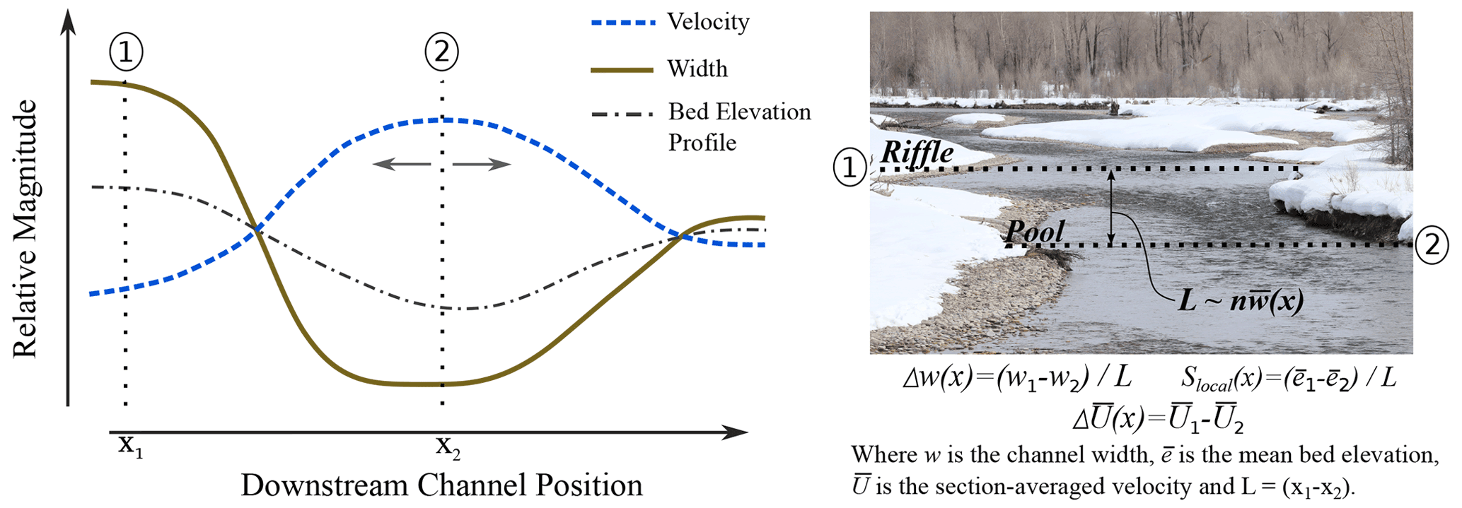
Figure 1 Conceptual diagram illustrating an inverse correlation between channel width and the width-average flow velocity (or the local shear velocity) and the likely resulting bed topography profile. The inverse correlation has been shown to occur along river segments and has been reproduced by numerical simulations of pool–riffle sequences and analogue physical experiments (Thompson et al., 1999; de Almeida and Rodríguez, 2012; Bolla Pittaluga et al., 2014; Nelson et al., 2015; Chartrand et al., 2018). The gray arrows indicate that the location of the velocity maxima (and minima) shifts depending on the flow stage (Wilkinson et al., 2004). The photograph on the right shows a gravel bed river in the spring rising snowmelt stage with a width gradient from points 1 to 2 over a distance $n\stackrel{\mathrm{‾}}{w}\left(x\right)$, where n can vary from 1 and higher. Bed architecture at point 1 is a riffle and is a pool at point 2. Flow direction is from the top to the bottom of the image. Note the broken water surface as flow transitions into the narrower location at point 2. Photograph by Shawn M. Chartrand, Flat Creek, near Jackson Hole, WY, USA.

Downstream differences in the width-averaged flow velocity and near-bed shear stress give rise to varying momentum fluxes delivered to the gravel bed surface. Over years to decades or longer, the fluctuating magnitude of momentum fluxes associated with flood and sediment supply events of varying magnitude and duration (intensity) shapes the local bed topography and surface grain size distribution through sediment particle entrainment and deposition (Chartrand et al., 2019) and bed load transport more generally (e.g., Church, 2006). Event-specific feedbacks between the flow, bed topography, bed sediment texture, and bed load transport continually refine and further shape local bed architectures (Leopold et al., 1964; Parker, 2007) and generally determine whether there is a tendency for net local deposition or erosion along pool–riffle sequences (Wilkinson et al., 2004; MacWilliams et al., 2006; de Almeida and Rodríguez, 2011, 2012; Brown and Pasternack, 2017; Chartrand et al., 2018). The combination of these factors provides a basic construct for the formation of pool–riffle sequences along gravel bed rivers with downstream width variations. At narrowing channel segments, flows speed up and deliver relatively higher momentum flux to the bed surface, leading to net erosion, whereas at widening segments flows slow down and deliver lower momentum flux, favoring net deposition (see Furbish et al., 1998). However, the specifics of how pool–riffle sequences respond to temporal changes in local width conditions and evolve to statistically steady-state bed topography are largely unexplored. This knowledge gap has implications for anticipating and projecting gravel bed river responses to restoration actions and dam removal (East et al., 2015; Gartner et al., 2015; Magilligan et al., 2016; Harrison et al., 2018; De Rego et al., 2020); coarse sediment management at upstream reservoirs (Chartrand, 2022); and effects related to climate change that are likely to influence basin hydrology, the intensity and magnitude of flood events, and sediment production (East and Sankey, 2020).

Here, we make progress using scaling theory understood through an analogue experiment, the results of which are in line with an extensive data set drawn from the literature. We address two research questions through our analysis. First, how does a pool–riffle channel segment respond to local temporal changes in channel width? Second, do resultant topographic adjustments conform to expectations of an inverse correlation between the local dimensionless downstream width gradient Δw(x) and bed slope S_local(x) (Fig. 1)? The width gradient is calculated as the quotient of the downstream width difference between two points where the direction of width variation changes, divided by the downstream distance between these points. The bed slope is calculated as the quotient of the bed elevation difference between the same two points where the direction of width variation changes, also divided by the downstream distance between these points. An inverse correlation in the present sense provides two possible conditions: −Δw(x) (downstream narrowing) with +S_local(x) (positive downstream slope) and +Δw(x) (downstream widening) with −S_local(x) (negative or adverse downstream slope) (see Brown and Pasternack, 2017, for a complementary discussion). To this end, the paper is structured in the following way. In the next section we present a scaling argument that offers a general explanation for the inverse correlation between the local downstream width gradient Δw(x) and bed slope S_local(x). Local bed slope is a basic descriptor of topographic conditions, and collectively over many mean widths in length describes the bed architecture. Following an explanation of the scaling theory, we describe the physical experiment and then present our results, followed by a discussion of the implications of our work with respect to natural rivers. Throughout the text we refer to spatial differences in channel width as “variations” and temporal differences of channel width at specific locations as “changes”.

We show that adjustments of local bed slope following prescriptive temporal changes to channel width generally follow an expected inverse correlation. This outcome is consistent with a new and expanded data set drawn from the literature representing available field-based studies and results from numerical analyses and analogue experiments (n=88). The expanded field-based data sets motivated a more careful consideration of profile responses to associated width variations. We find that actions such as dam removal, which impulsively increases the supply of bed load sediment to downstream river reaches, can cause a transient flipping of the expected inverse correlation between the local downstream width gradient and bed slope due to pool filling (e.g., Lisle and Hilton, 1992) and smoothing of the local topographic profile. The timing and sequence of hydrograph events post dam removal may also play a role in downstream bed profile dynamics (Nelson et al., 2015; Morgan and Nelson, 2021). We use the transient flipping of the expected inverse correlation between Δw(x) and S_local(x) to expand interpretation of the proposed scaling theory and suggest further context for expected short-term river dynamics associated with dam removal and similar transient events that disrupt upstream coarse-sediment supplies (Cui et al., 2006; East et al., 2015; De Rego et al., 2020).

2 Theory

Assuming steady-state conditions, the local bed slope S_local(x) between two points where the direction of width variation changes along a river profile can be expressed as the product of two terms (see Chartrand et al., 2018, for more details regarding assumptions and derivation):

$$\begin{array}{}\text{(1)}& S_{\mathrm{local}}\left(x\right)\sim \mathrm{\Lambda }\left(\mathit{\Delta }{\stackrel{\mathrm{‾}}{U}}_x^{\ast }\right).\end{array}$$

The bed architecture stability parameter Λ sets the relative magnitude of the local channel profile in terms of characteristic timescales for the flow t_f and gravel bed river topographic adjustment t_y:

$$\begin{array}{}\text{(2)}& \mathrm{\Lambda }=\underset{\mathrm{1}/t_y}{\underbrace{\left({\displaystyle \frac{[{\mathit{\rho }}^{\prime }g{D}_{\mathrm{90}f}{]}^{\mathrm{0.5}}}{\mathit{\epsilon }w}}\right)}}\underset{t_f}{\underbrace{\left({\displaystyle \frac{D_{\mathrm{90}f}}{u^{\ast }}}\right)}}={\displaystyle \frac{t_f}{t_y}},\end{array}$$

where ${\mathit{\rho }}^{\prime }=\left[\right({\mathit{\rho }}_{\mathrm{s}}/{\mathit{\rho }}_{\mathrm{w}})-\mathrm{1}]$, ρ_s=2650 kg m⁻³ is the density of sediment, ρ_w = 1000 kg m⁻³ is the density of water, g=9.81 is the acceleration of gravity, D_90f is the grain size for which 90 % of all particles of the sediment supply are smaller, $\mathit{\epsilon }=(\mathrm{1}-\mathit{\varphi })$ is the solid fraction in the bed, ϕ=0.4 is the volume-averaged streambed porosity of the active layer L_a=kD_i (Hirano, 1971), k is constant between 1 and 2 (Parker, 2008), w is the local channel width, and u_∗ is the local shear velocity defined as $(g\stackrel{\mathrm{‾}}{d}S{)}^{\mathrm{0.5}}$, where $\stackrel{\mathrm{‾}}{d}$ is the width-averaged water depth.

Here, the topographic adjustment time is a timescale for particle mixtures to aggregate or disaggregate and is a metric for the tendency for sediment particle deposition or entrainment, respectively. The topographic adjustment time t_y is set by the relative mass (i.e., size) of the D_90f, the packing condition of the bed surface sediments which governs particle–particle stress coupling and the local channel width. The flow time t_f indicates the intensity of momentum flux delivered to the gravel bed surface (cf. Yalin, 1971; Carling and Orr, 2000). The flow time is set by the magnitude of the shear velocity in comparison to the relative mass of the D_90f. Critically, Λ identifies an inherent covariation between the flow velocity and channel width that governs the resilience of pool–riffle bed architecture (see the updated discussion of pool–riffle maintenance in Morgan and Nelson, 2021) (Fig. 1).

The dimensionless velocity change $\mathit{\Delta }{\stackrel{\mathrm{‾}}{U}}_x^{\ast }$ quantifies the acceleration between two locations moving downstream where width change occurs:

$$\begin{array}{}\text{(3)}& \mathit{\Delta }{U}_x^{\ast }={\stackrel{\mathrm{‾}}{U}}_x^{\ast }\left(x\right)-{\stackrel{\mathrm{‾}}{U}}_x^{\ast }(x+\mathit{\Delta }x),\end{array}$$

and specifically,

$$\begin{array}{}\text{(4)}& {\stackrel{\mathrm{‾}}{U}}_x^{\ast }=\left({\displaystyle \frac{{\stackrel{\mathrm{‾}}{U}}_x}{{\left({\mathit{\rho }}^{\prime }g\stackrel{\mathrm{‾}}{d}\right)}^{\mathrm{0.5}}}}\right),\end{array}$$

where ${\stackrel{\mathrm{‾}}{U}}_x^{\ast }$ is a dimensionless wave speed or Froude number $\mathit{Fr}={\stackrel{\mathrm{‾}}{U}}_x/(g{L}_{\mathrm{c}}{)}^{\mathrm{0.5}}$, the square of which expresses a balance between (a) the kinetic energy available in the velocity field to do work to deform the bed and (b) the restoring potential energy in the bed topography. The parameter ${\stackrel{\mathrm{‾}}{U}}_x$ is the width-averaged flow velocity and L_c a characteristic length. Local downstream gradients of dimensionless bed load transport vary inversely with dimensionless velocity gradients related to the role of $\stackrel{\mathrm{‾}}{d}$ in setting the magnitude of $\mathit{\Delta }{\stackrel{\mathrm{‾}}{U}}_x^{\ast }$, for example $\mathit{\Delta }{q}_{b_x}^{\ast }\sim -\mathit{\Delta }{\stackrel{\mathrm{‾}}{U}}_x^{\ast }$ (see Chartrand et al., 2018). Consequently, we assume that profile disturbances propagate at a wave speed that scales as spatial differences in ${\stackrel{\mathrm{‾}}{U}}_x^{\ast }$. Positive differences in ${\stackrel{\mathrm{‾}}{U}}_x^{\ast }$ drive profile changes upstream to downstream, and negative differences have the opposite effect. In relation to S_local(x), a key take away is that the sign of $\mathit{\Delta }{\stackrel{\mathrm{‾}}{U}}_x^{\ast }$ is determined on the basis of how downstream differences between ${\stackrel{\mathrm{‾}}{U}}_x$ and $\stackrel{\mathrm{‾}}{d}$ compare. As a result, this parameter captures how velocity and depth comparatively respond to downstream width changes, which itself could be dependent upon local bed surface texture conditions or spatial patterns of bed topography (Wolman, 1955). These points highlight how the effects of downstream width change are implicitly represented in Eq. (1), bridging a connection with Fig. (1). For the experiments discussed next we treat channel width and its local changes as an independent, random variable, and the local bed slope as a dependent, random variable.

3 Experimental design and methods

Here, we present a new analogue experiment referred to as Pool–Riffle Experiment 4 (PRE4) and revise and analyze in greater detail an extensive series published previously (Chartrand et al., 2018, 2019; Hassan et al., 2021). PRE4 was designed specifically to characterize local bed topographic responses to locally specific temporal changes in channel width after approximate topographic steady-state conditions were achieved. The pre- and post-width change periods are referred to as Phases 1 and 2, respectively (Table 1). This transient experiment was accomplished by manually adjusting the positions of rigid plywood channel walls inset within a flume over a centrally located segment of roughly 3 m (Fig. 2). This basic setup provided for experimental conditions with two distinct downstream channel width configurations for the region of interest, characterized by associated patterns of downstream width variations (Fig. 2c). The Phase 2 downstream width variation configuration was used for prior experiments (Chartrand et al., 2018) and includes a prominent widening and narrowing sequence. We choose to focus on a flume segment with relatively large downstream width variations based on the hypothesis that a measurable response would occur and thus facilitate testing against prior results and Eq. (1) (Fig. 2c).

Table 1 Experimental details for PRE4.

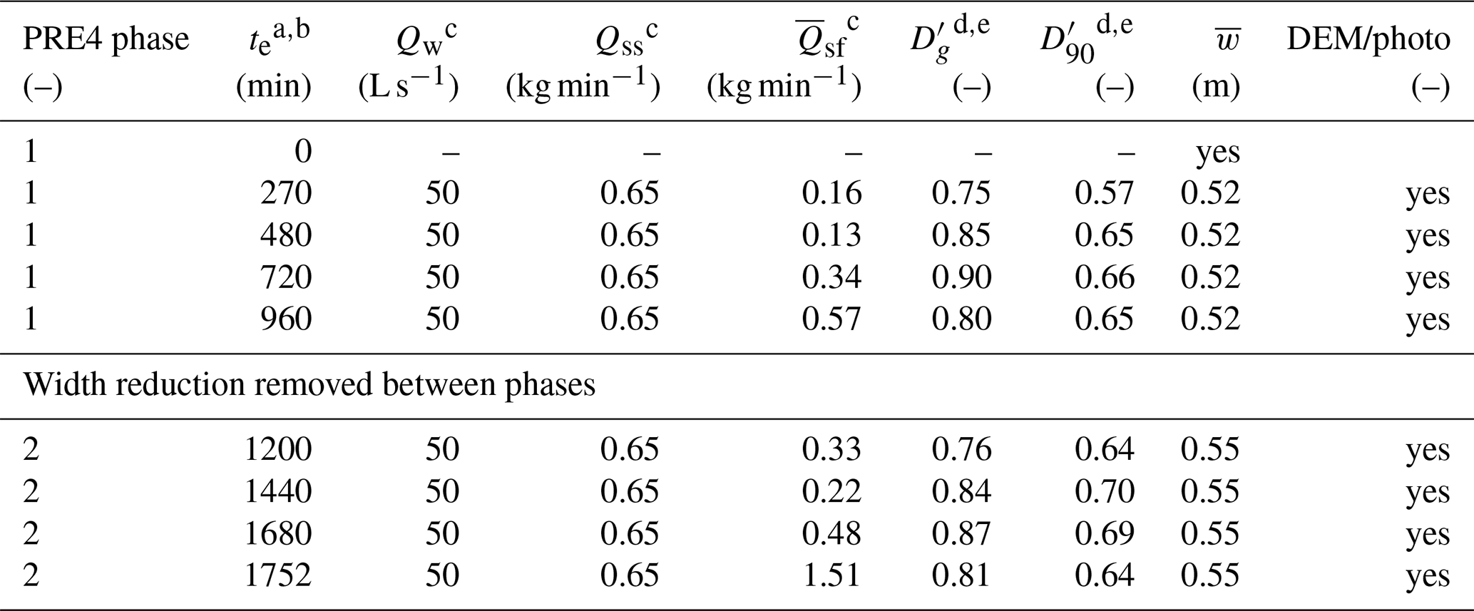
^a t_e is the elapsed time, which indicates the end time for the specified interval. ^b At the elapsed times shown, upstream supplies were stopped, the flume was drained, and measurements were made. ^c Q_w is the water supply rate, Q_ss is sediment supply rate, and ${\stackrel{\mathrm{‾}}{Q}}_{\mathrm{sf}}$ is the time-averaged sediment flux at flume outlet. ^d Grain size metrics are for the sediment flux at the flume outlet. ^e ′ denotes normalized by sediment supply grain size.​​​​​​​

Figure 2 Experimental design of channel width gradients for Phases 1 and 2 of PRE4. (a) Overhead view of the Phase 1 experimental channel showing how channel width changes in the downstream direction. Phase 1 ended at elapsed time 960 min (see Table 1). (b) Overhead view of the Phase 2 experimental channel showing how channel width changes in the downstream direction. Phase 2 began following Phase 1. Color shading for both (a) and (b) represents a relatively smoothed elevation condition for illustration only. The Phase 2 width configuration corresponds to the setup reported by Chartrand et al. (2018). (c) Downstream channel width gradients for Phases 1 and 2, connected by lines for illustration only. Points are plotted at locations that correspond to the red squares of (a), which set the downstream differencing length scale and locations where mean local width was calculated. Values above the zero-width gradient line represent widening conditions, and those below this line represent narrowing. The dashed red polygon highlights the location from approximately station 10.6 to 8.15 m where the bank positions were manipulated at elapsed time 960 min as per the experimental design.

PRE4 was conducted in a 15 m long and 1 m wide flume, with downstream variations of channel width modeled from a 75 m long reach of East Creek, University of British Columbia Malcolm Knapp Research Forest, BC, Canada. The field prototype is a small, gravel bed stream with pool and riffle bed architecture along the model reach. The experimental channel sidewalls were inset within the larger flume and constructed from rough-faced veneer-grade D​​​​​​​ plywood with a surface roughness ranging from 1 to 4 mm. Water and sediment were supplied at the upstream end of the flume, and water was recirculated via a pump. Sediment was introduced at the upstream end of the flume via a conveyor system and was captured at the downstream end of the flume in a wire mesh basket. Prior to capture, sediment sizes of the time-averaged transported load were estimated using a light table imaging device (Frey et al., 2003; Zimmermann et al., 2008; Chartrand et al., 2018).

Both the sediment supply and flume bed sediments had the same distribution of sizes ranging from 0.5 to 32 mm, with a geometric mean grain size of 7.3 mm and a D₉₀ of 21.3 mm. Bed topography was captured using a camera–laser system with a resolution of 1 mm in the longitudinal, lateral, and vertical planes. Width variations of the experimental flume provide a range of downstream channel width gradients Δw(x) ranging from −0.26 to +0.47 (Fig. 2c). The largest local width measured 0.758 m at station 9.960 m (during Phase 2) and the smallest width measured 0.37 m at station 8.150 m (both phases). The Phase 1 downstream width configuration had a mean width $\stackrel{\mathrm{‾}}{w}$ of 0.52 m, and the Phase 2 configuration had a mean width of 0.55 m. Phase 1 of PRE4 was conducted with a width reduction in place, and Phase 2 was done with it removed (Table 1 and Fig. 2). At the start of PRE4 Phase 1 we installed two pieces of plywood to connect bank positions from station 10.625 to 8.150 m, producing a negative width gradient between these locations of −0.06 – i.e., a gradual linear narrowing of the channel. The flume bed was then smoothed to a near-constant downstream bed slope of +0.015. Next, we ran water flow at 50 L s⁻¹ and supplied sediment at the approximate transport capacity and mass flow rate of 0.65 kg min⁻¹. The water flow rate scales as slightly higher than an assumed 2-year return period flood in East Creek.

Figure 3 Experimental conditions at approximate topographic steady-state times during PRE4 for Phases 1 and 2. (a) Photographs at elapsed times of 960 and 1752 min, taken just downstream of the narrowest channel segment. The location of the installed plywood to narrow the channel from station 10.6–8.15 m is highlighted. There is a water supply of 5 L s⁻¹ for the image on the left and 2 L s⁻¹ for the image on the right. (b) Bed topography at elapsed time 960 min. Red squares show locations where channel width and bed elevation were sampled to understand correlations between downstream width change and local bed slope. (c) Topographic profile at elapsed time 960 min (thick black line), with the profile at 720 min shown for discussion (thin orange line). (d) Bed topography at elapsed time 1752 min. The bank positions were adjusted from station 10.6 to 8.15 m, denoted by the dashed red polygon. (e) Topographic profile at elapsed time 1752 min (thick black line), with the profile at 1680 min shown for discussion (thin orange line). Water surface profiles were smoothed using a downstream windowed mean over a length scale of 0.5 m. Topographic profiles were spatially averaged from digital elevation models for a centered cross-stream length scale of 0.160 m. Zero crossing lines are calculated per Richards (1976). “P” stands for pool and “R” for riffle, with smaller font used for more subtle features.

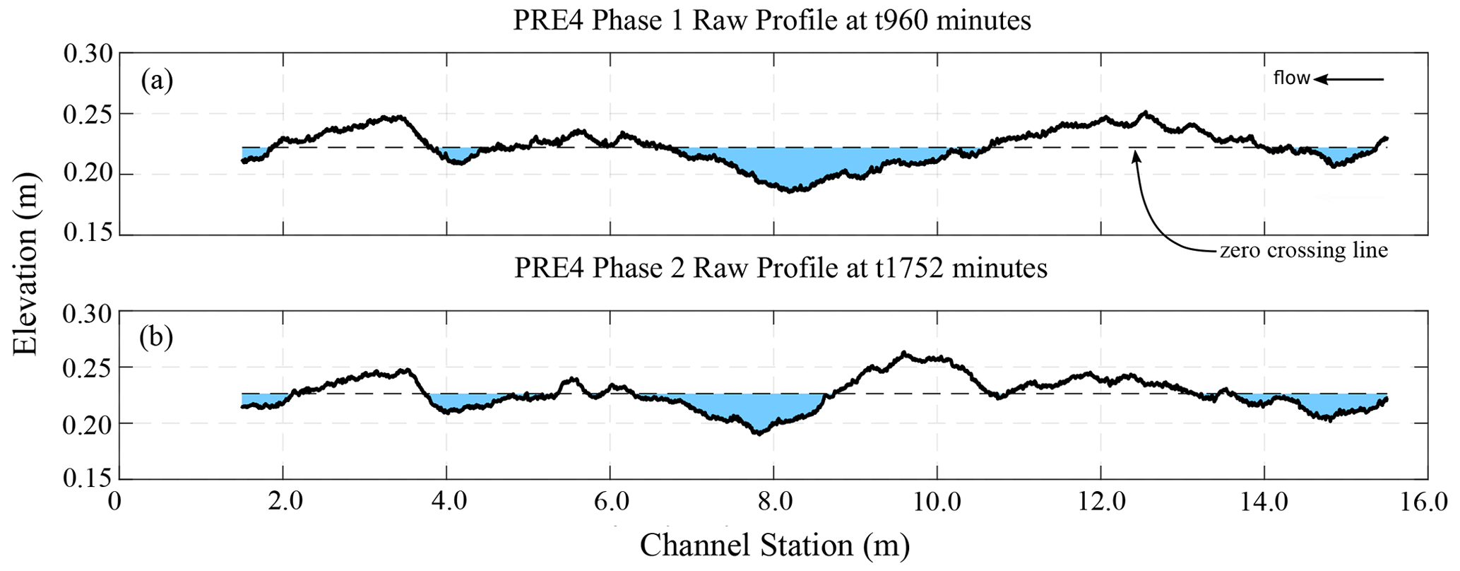
Figure 4 Detrended bed elevation profiles showing a zero-crossing line for Phases 1 and 2 of PRE4. (a) Bed elevation profile at t960 min and (b) t1752 min, each calculated as width-averaged elevations at a resolution of 2 mm. Both profiles are fit with a zero-crossing line (Richards, 1976). The elevation profiles do not have a trend and were sampled from the raw digital elevation models (see Chartrand et al., 2018, for more details regarding measurement methods for flume bed elevations). Pool-like features are shown with blue shading below the zero-crossing line.

Phase 1 was complete when approximate topographic steady state was achieved at elapsed time 960 min (compare orange and black profiles in Fig. 3c and see the video in the online repository). At this stage the plywood pieces from station 10.625 to 8.150 m were carefully removed to minimize disturbance of the bed surface sediments and local topography, and sediment was added to the regions that were located behind the plywood walls to match the local Phase 1 bed slope. We then started Phase 2 of PRE4 by resuming the same upstream water and sediment supply rates used during Phase 1. Phase 2 was carried out until approximate topographic steady state was achieved at an elapsed time of 1750 min (compare orange and black profiles in Fig. 3e and see the video in the online repository). Measurements were made at several points during Phases 1 and 2 of the experiment: elapsed times 270, 480, 720, 960, 1200, 1440, 1680, and 1752 min (Table 1). To facilitate measurements, the water and sediment supplies were stopped, and the flume was drained at the indicated times. In the discussion below we address a pool feature as the bed surface that occurs below the zero-crossing line, and a riffle feature is that which occurs above the same line (Richards, 1976) (Fig. 4a and b). Different morphologic classification systems exist (e.g., Carling and Orr, 2000; Wyrick et al., 2014), but here we choose a basic definition to reflect that we ran analogue experiments to natural settings.

4 Results

4.1 Topographic response to changes in width

Figure 3 shows images, digital elevation models (DEMs), and profiles of experimental conditions at the end of Phases 1 and 2 of PRE4. At the end of Phase 1 the bed topography of the experimental channel consisted of the following sequence of features from upstream to downstream: pool–riffle–pool–riffle–pool–riffle (Fig. 3b and c). Riffle features during Phase 1 are colocated with zones of channel widening, and pool features are colocated with zones of channel narrowing (Fig. 3b and c). The downstream width gradients associated with these topographic features range from −0.09 to +0.47, narrowing and widening, respectively (Fig. 2c). The riffle–pool sequence from stations 13 to 7 m was the most prominent topographic feature of Phase 1 with a maximum elevation difference from riffle to pool of approximately 0.07 m (Figs. 3b and c and 4a), and downstream width gradients of +0.07 and −0.06, respectively (Fig. 2c). This riffle–pool unit is illustrated in the left image of Fig. 3a. Differences relative to the zero-crossing line indicate that the riffle had a maximum amplitude of approximately +0.024 m, which occurred at station 12.6 m, whereas the pool had a maximum amplitude of −0.045 m, which occurred at station 8.3 m (Fig. 4a). An additional riffle feature was observed with its crest near station 3.7 m, with a maximum amplitude of +0.025 m. Less pronounced pool features formed at two other locations centered around stations 15.0 and 4.1 m.

At the end of Phase 2 the bed topography consisted of the following sequence of features from upstream to downstream: pool–riffle–riffle–pool–riffle (Fig. 3d and e). As with Phase 1, riffle and pool features during Phase 2 are colocated with zones of widening and narrowing, respectively, for width gradients ranging from −0.26 to +0.47 (Fig. 2c). The riffle–pool unit from stations 10.8 to 7 m was the most prominent topographic feature of Phase 2, with a maximum elevation difference from riffle to pool of approximately 0.07 m (Figs. 3d and e and 4a) and downstream width gradients of +0.35 and −0.26, respectively (Fig. 2c). This riffle–pool unit is illustrated in the right image of Fig. 3a. Differences relative to the zero-crossing line indicate that the riffle had a maximum amplitude of approximately +0.035 m, which occurred at stations 9.7 to 10 m, whereas the pool had a maximum amplitude of −0.037 m, which occurred at station 7.8 m (Fig. 4b). As with Phase 1, an additional riffle feature was observed with its crest near station 3.7 m, with a maximum amplitude of +0.02 m, and an additional riffle is observed centered around station 12 m. This feature has a maximum amplitude of +0.021 m (Fig. 4a). Two additional pool features formed at locations centered around stations 15.0 and 4.1 m.

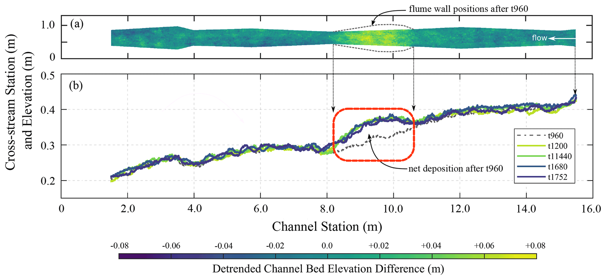
Figure 5 Bed elevation and profile changes after the width reduction was removed. (a) DEM of difference between t960 and t1200 min. The width profile for t960 min used to show elevation differences because it was narrower within the central part of the flume compared to t1200 min. Width profile following t960 min is shown with the light gray lines. (b) Trended mean channel bed profiles for t960, t1200, t1440, t1680, and t1752 min. The dashed red box lines up with region where the width reduction was removed following t960 min. Profiles calculated as width-averaged conditions with a resolution of 0.002 m.

Figure 5 shows a DEM of difference (DoD) between elapsed times 960 and 1200 min and width-averaged channel bed elevation profiles for elapsed times 960, 1200, 1440, 1680, and 1752 min. Following removal of the width reduction at t960 min, bed elevation conditions adjusted through deposition focused within the central part of the flume where the width reduction was removed (Figs. 3 and 5a and b). Over the course of 240 min following elapsed time t960 min, a width-averaged depth of 0 to 0.06 m of sediment was deposited between stations 10.6 to 8.1 m, with maximum deposition depths centered around stations 9.9 and 9.1 m (Fig. 5b). At the resolution of the underlying DEMs, deposition was spatially variable over the central region and tapers off in the upstream and downstream directions (Fig. 5a). Outside of the region between stations 10.6 to 8.1 m, bed elevation profiles are comparable prior to and after the width reduction was removed. Furthermore, following an elapsed time of t1200 min, adjustment of the elevation profile was relatively minor, with width-averaged differences ranging from 0.004 to 0.007 m (Fig. 5b), smaller than the geometric mean grain size.

4.2 Covariation of width change and local bed slope

Figure 6 shows how local bed slopes vary according to associated downstream width gradients and has four quadrants that describe the correlation between S_local(x) and Δw(x). The upper-left and lower-right quadrants mark inverse correlations, whereas the upper-right and lower-left describe direct correlations. Phase 1 and 2 results of PRE4 are broken down into two separate categories for plotting: (1) sites at which the width gradient changes between Phases 1 and 2 and (2) sites at which the width gradient is fixed for both phases of PRE4.

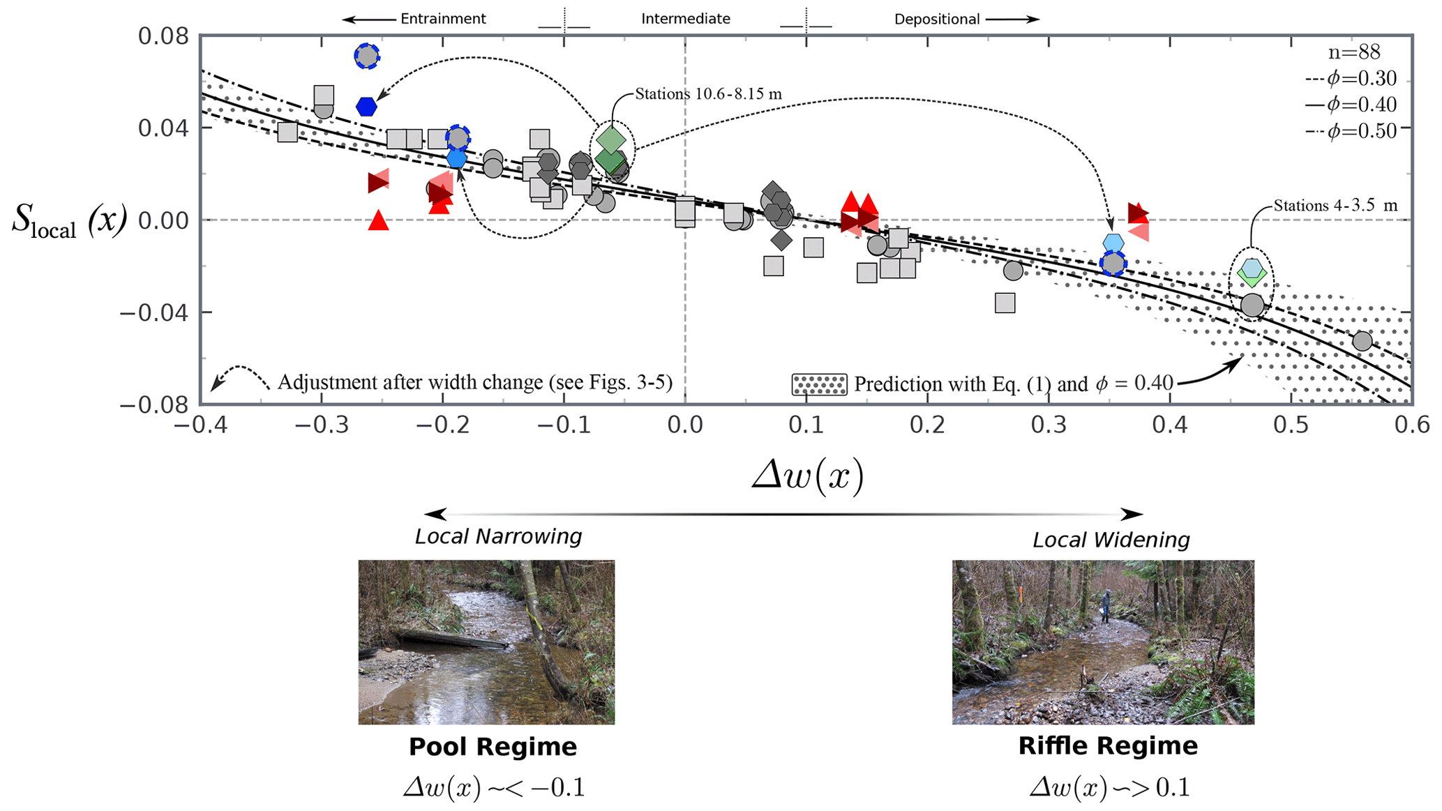
Figure 6 Local average bed slope S_local(x) as a function of the downstream channel width gradient Δw(x) for PRE4 and a wide range of additional field, numerical, and experimental studies. For the present experiment the symbols are used in the following way: the green diamond​​​​​​​ shows Phase 1 PRE4 and the blue hexagon shows Phase 2 PRE4 at locations where channel width is adjusted during the experiment, the dark gray diamond shows Phase 1 PRE4 and the dark gray hexagon shows Phase 2 PRE4 at locations where width remains unchanged during the experiment, and the light gray circle with dashed blue outline shows the result from Chartrand et al. (2018), which is comparable to PRE4 for the same downstream width gradient. For the literature-based data sets the symbols are used in the following way: the light gray circle represents Chartrand et al. (2018), which includes data from Thompson et al. (1999) (field), de Almeida and Rodríguez (2012) (numerical), Bolla Pittaluga et al. (2014) (numerical), and Nelson et al. (2015) (experiment); the light gray square includes data from Richards (1976) (field), Cao et al. (2003) (numerical), and Vahidi et al. (2020) (experiment). The pink triangle represents the period before the Elwha and Glines Canyon dams were removed on the Elwha River, the red triangle shows data following the removal of the Elwha dam and all but 9.1 m of the Glines Canyon dam in the spring prior to the freshet floods, and the dark red triangle shows data taken in the late summer after the freshet floods and with the remaining 9.1 m of Glines Canyon dam still in place. All three of these use data from Brew et al. (2015) (field). See Appendix A for more details regarding the literature-based data sets (light gray squares). Plotted lines represent the center of a distribution of predicted values using Eq. (1) for differing values of the packing fraction ε. See Appendix A and the online repository (Chartrand et al., 2022) for the calculation procedure of Eq. (1). The distribution of predicted values is shown with hatching for ϕ=0.40.

Local bed slope and width gradients for both phases of PRE4 are consistent with expectations of an inverse correlation between Δw(x) and S_local(x) of Eq. (1). At locations where the width gradient changes during the experiment, the Phase 1 steady-state topographic conditions converge at $\mathit{\Delta }w\left(x\right)=-\mathrm{0.06}$, and S_local(x) ranges from +0.026 to +0.035. Following adjustment of the downstream width gradients at the start of Phase 2 (Fig. 2c), the Phase 1 steady-state topographic conditions evolve according to the prescribed width changes: $\mathit{\Delta }w\left(x\right)=-\mathrm{0.26}$ and $S_{\mathrm{local}}\left(x\right)=+\mathrm{0.49}$, $\mathit{\Delta }w\left(x\right)=-\mathrm{0.19}$ and $S_{\mathrm{local}}\left(x\right)=+\mathrm{0.27}$, and $\mathit{\Delta }w\left(x\right)=+\mathrm{0.35}$ and $S_{\mathrm{local}}\left(x\right)=-\mathrm{0.01}$. At locations where the width gradients were fixed over the duration of PRE4, the Phase 1 and 2 bed slopes are similar. For example, stations 4–3.5 m at steady-state $S_{\mathrm{local}}\left(x\right)=-\mathrm{0.23}$ for Phase 1 and −0.21 for Phase 2 (Fig. 6). The trend of local bed slopes for PRE4 across the downstream width gradient parameter space corresponds to the scaling theory (Eq. 1) before and following the width changes (Fig. 3). More generally, the scaling theory projects a nonlinear slope response for downstream width gradients, with a tendency toward flat segments of bed at $\mathit{\Delta }w\left(x\right)\sim +\mathrm{0.10}$. For width gradients away from this transition point, projections of local bed slope are increasingly positive and negative for narrowing and widening channel segments, respectively, and correlates with the bed packing condition ε.

Data sets from published field studies and numerical and analogue experiments generally agree with expectations of an inverse correlation between S_local(x) and Δw(x) (n=88). On the basis of Eq. (1), data for natural rivers with reported downstream width variations include the river Fowey, Cornwall, UK (Richards, 1976), North Saint Vrain Creek, CO, USA (Thompson et al., 1999), and the Elwha River, WA, USA (Brew et al., 2015). Data for numerical experiments with downstream width variations include de Almeida and Rodríguez (2012), Bolla Pittaluga et al. (2014), and Cao et al. (2003). Data for analogue experiments with downstream width variations include Nelson et al. (2015), Chartrand et al. (2018), and Vahidi et al. (2020). A few studies merit specific mention. Bed slope responses for PRE4 show strong agreement with prior experimental results completed with the same setup, but for which the downstream sequence of channel width was fixed (Chartrand et al., 2018). In particular, PRE4 local steady-state bed slopes following the prescribed width changes are consistent with prior outcomes for the same downstream width gradients and are also consistent at locations where width gradients were unchanged for the duration of the experiments, for example, at stations 4–3.5 m (Fig. 6). Results of monitoring downstream bed elevation conditions before and during removal of the Elwha and Glines Canyon dams on the Elwha River show a range of local bed slope responses. Before dam removal S_local(x) and Δw(x) were inversely correlated (20 July 2011). After removal of the Elwha dam and during staged removal of the Glines Canyon dam, S_local(x) and Δw(x) were directly correlated at three of six sites (May 2013) following the first winter runoff season. Several months later and following the first summer snowmelt runoff season S_local(x) and Δw(x) were inversely correlated at four of six sites (Fig. 6) (August 2013).

5 Discussion and applications to natural rivers

Our scaling theory makes explicit predictions for local S_local(x) and Δw(x) conditions favoring the deposition of material to the bed to form riffles (Δw(x) ∼ > 0.10), the erosion of material from the bed to form pools (Δw(x) ∼ < −0.10), and intermediate regimes where both processes occur in concert (Δw(x)⇒0) (Fig. 6). Accordingly, here we discuss the primary implications of our combined results and theoretical expectations for natural rivers, including the importance of local width conditions and transient watershed processes that can contribute to time-varying bed slope responses. The PRE4 experimental channel exhibits distinct topographic patterns between Phases 1 and 2 that are correlated to the specific downstream patterns of channel width variation (Figs. 3, 4 and 6). During Phase 1 the upper and central portion of the experimental channel from stations 14–7 m included a zone of expansion followed by a relatively long zone of narrowing. This downstream organization of channel width led to development of a prominent pool–riffle–pool topographic response. Despite the moderate width gradient −0.06, the pool feature had the largest associated amplitude of the experiment, −0.045 m, according to the zero-crossing line method (Richards, 1976). During Phase 2 the width was adjusted from stations 10.6 to 8.1 m to include an abrupt zone of widening, +0.35, and then narrowing, −0.19 and −0.26. This change led to development of a prominent riffle–pool sequence, whereas in Phase 1 this region was occupied by a riffle tail transitioning to a pool. The Phase 2 zone of widening resulted in a riffle with the largest overall amplitude of the experiment, +0.35 m, and the pool had a marginally smaller amplitude compared to the Phase 1 pool of the same location, −0.035 m.

These results are important because they demonstrate that topographic responses within variable-width channel segments are strongly controlled by the quantitative character of width change (Richards, 1976; Cao et al., 2003; MacWilliams et al., 2006; de Almeida and Rodríguez, 2012; Nelson et al., 2015; Chartrand et al., 2018). More specifically, results for our geometrically simple experimental setups, as well as for literature-based data sets of Fig. 6 (see Appendix B), indicate that inflections in the profile curvature are generally locked with associated points or regions where the width gradient changes direction (Fig. 3): high points (riffles) along a profile are commonly aligned near places where a widening segment changes to a narrowing one and low points (pools) near places where a narrowing segment changes to a widening one. This outcome is explained by the scaling theory Eq. (1) as width-regulated feedbacks of local hydrodynamics and momentum exchange between the flow and the bed (Furbish et al., 1998), and consequently bed load sediment transport, depending on the grain size composition of the upstream sediment supply and the local bed packing state (also see Cao et al., 2003; Wilkinson et al., 2004; Bolla Pittaluga et al., 2014; Ferrer-Boix et al., 2016; Chartrand et al., 2018, 2019).

The spatial correlation between the local channel width gradient and bed slope includes comparatively more nuanced information that is important and merits discussion. For example, although a local width minimum at station 8.15 m did not change between Phases 1 and 2, the zone of maximum depth in the associated pool feature shifted its relative position. During Phase 1 the point of maximum amplitude in the pool occurred upstream of the location of minimum width at station 8.2 m, whereas it occurred downstream of the minimum width location during Phase 2 at station 7.8 m (Figs. 3 and 4). This result highlights that differing downstream configurations of width change can influence subtle aspects of pool morphology and dynamics (Carling and Wood, 1994; Thompson et al., 1998; Cao et al., 2003; Wilkinson et al., 2004; Thompson and McCarrick, 2010). Furthermore, a novelty of the topographic adjustments observed for PRE4 is the demonstration that simple manipulations of experimental width conditions for steady upstream supplies of water and sediment can yield a surprisingly diverse set of responses, which are consistent with expectations of the scaling theory (Fig. 6). However, unsteady upstream supplies of water and sediment also yield relatively large pool–riffle topographic responses (e.g., Lisle and Hilton, 1992; Brew et al., 2015; East et al., 2015; Vahidi et al., 2020; Morgan and Nelson, 2021), including lateral channel shifting and re-activation due to pool filling (e.g., East et al., 2015) and reduction of topographic (bar–pool) amplitude (Morgan and Nelson, 2021). The critical take away here is that local channel width conditions matter (Nelson et al., 2015; Brown and Pasternack, 2017; Chartrand et al., 2018), the context of which provides a rich understanding for general topographic and bed architecture conditions within gravel bed rivers. Similar importance is also attributed to downstream variations in valley width in relation to the longitudinal profile of riffle–pool river segments (Sawyer et al., 2010; White et al., 2010). Accordingly, explicit or implicit spatial averaging of channel and bed architecture geometry over distances that are greater than that describing local width variations can mask the correlations demonstrated here (Fig. 6). For example, consider the Phases 1 and 2 flume-wide average channel widths of 0.52 and 0.55 m, respectively. Averaging the bed profiles of Fig. 3 over the flume length yields slopes of 0.014 and 0.014, respectively. Consequently, identical bed slopes occur for similar flume-wide average channel width conditions and the same upstream water and sediment supplies, demonstrating a loss of information relative to the results presented here (Byrne et al., 2021).

A range of factors or processes not easily captured by the present scaling theory (Eq. 1) are relevant to setting the time-dependent local bed slope and are therefore important for understanding gravel bed river channel morphology. Specifically, factors that contribute to and may potentially overprint width-variation-driven downstream bed slope differences include effects of the stochastic nature of bed load transport (e.g., Furbish and Doane, 2021; Hassan et al., 2022), which make explicit “local” definitions of the flow timescale t_f and the bed adjustment timescale t_y challenging. However, Eqs. (2) and (4) indicate that the local bed slope at or near steady state is set by how the coarse fraction of the bed surface compares to the bed packing fraction, width, and shear velocity, and in turn how, through Λ, these quantities compare to the dimensionless downstream velocity change. The key here is if any of these quantities show change for a relatively long period of time (e.g., ≫t_y or t_f), for example, due to a disturbance in the upstream sediment supply, it is likely that the steady-state bed slope as a result of this change will differ from the pre-disturbance condition. Figure 6 suggests that as long as the local width variation condition does change appreciably, the pre- and post-disturbance bed slopes will be comparable and have an inverse correlation with Δw(x). Second, identification of appropriate response scales for pool–riffle gravel bed rivers are made complicated if time-dependent variations in the upstream supply of sediment (Dolan et al., 1978; Lisle and Hilton, 1992, 1999; de Almeida and Rodríguez, 2011; Brew et al., 2015; Vahidi et al., 2020; Morgan and Nelson, 2021) and water (Brew et al., 2015; Nelson et al., 2015; Morgan and Nelson, 2021; see discussion by East et al., 2015) occur over timescales comparable to that associated with achieving steady-state topographic conditions because river segments are continually responding to upstream disturbances (Ferrer-Boix and Hassan, 2014). Finally, strong transient variations of local bed surface sediment texture (Dolan et al., 1978; Lisle, 1986) and bank material composition over length scales $<\stackrel{\mathrm{‾}}{w}$ (Wolman, 1955; Richards, 1976) or landsliding within river segments where valley wall processes are coupled to the channel (Whiting and Bradley, 1993; Hassan et al., 2019) can lead to new local channel widths and bed topographic responses where the latter is decoupled from the former. In particular, the influence of upstream sediment supply to local bed topographic responses has been studied extensively in the field and laboratory and may be a primary factor that influences the correlation between the local downstream width gradient and bed slope (Fig. 6) (see helpful discussions in East et al., 2015; Morgan and Nelson, 2021).

Previously it was unclear whether pools and riffles express direct correlations between Δw(x) and S_local(x) – i.e., the upper-right and lower-left quadrants of Fig. 6 (Chartrand et al., 2018; also see Brown and Pasternack, 2017, and note that their covariance convention differs in sign to the width gradient–slope parameter space reported here). Field-based observations prior to and following substantial removal of the Elwha and Glines Canyon dams on the Elwha River, WA, USA, suggest that an increase in the upstream supply of bed load sediment (see East et al., 2015) without a substantial local adjustment to the downstream pattern of channel width is sufficient for pool–riffle segments to have a relatively short-lived, site-specific direct correlation between the local downstream width gradient and bed slope (Fig. 6) (see Fig. 5 of Brew et al., 2015). For example, prior to dam removal a riffle located between stations 50 500–50 000 ft (15 392–15 240 m) (from the river mouth) had a local width gradient $\mathit{\Delta }w\left(x\right)=+\mathrm{0.137}$ and a local bed slope $S_{\mathrm{local}}=-\mathrm{0.003}$. Following removal of the Elwha dam and most of the Glines Canyon dam, the spring freshet transported an increased bed load sediment supply to the reach, resulting in a changed local bed slope of $S_{\mathrm{local}}=+\mathrm{0.008}$ and a site-specific direct correlation with the width gradient, i.e., upper-right quadrant of Fig. 6 with +Δw(x), +S_local(x). Following completion of the spring freshet and summer storm season, a site-specific inverse correlation was re-established with $S_{\mathrm{local}}=-\mathrm{0.001}$. A similar trend is observed for a riffle with $\mathit{\Delta }w\left(x\right)=+\mathrm{0.151}$ located between stations 51 488 and 50 935 ft (15 694–15 525 m). However, S_local does not quite reach negative or downstream adverse slope conditions following the spring freshet and summer storm season. On the other hand, a pool with $\mathit{\Delta }w\left(x\right)=-\mathrm{0.25}$ located between stations 50 935 and 50 590 ft (15 525–15 420 m) shows a significant response to the dam removal but does not quite express a site-specific direct correlation. Prior to dam removal and following the spring freshet and summer storm season, $S_{\mathrm{local}}\sim +\mathrm{0.018}$. During the spring freshet the local bed slope decreases considerably due to pool filling through sediment deposition and has an approximately flat downstream profile. At the end of the runoff season, local bed slope has recovered to near pre-dam-removal conditions with $S_{\mathrm{local}}\sim +\mathrm{0.016}$. These results highlight that the observations of Brew et al. (2015) and East et al. (2015) and also the numerical and physical experiments of Cao et al. (2003), Wilkinson et al. (2004), MacWilliams et al. (2006), de Almeida and Rodríguez (2011, 2012), Vahidi et al. (2020), and Morgan and Nelson (2021) are important because they provide evidence that pool–riffle river segments can exhibit a broad and dynamic range of conditions between downstream channel width gradients and bed topography depending on the upstream supplies of water and sediment. In particular, the Elwha River data set suggests it is possible for pools and riffles to exhibit a relatively short-lived direct correlation between Δw(x) and S_local(x) (see Brown and Pasternack, 2017, for more discussion of direct correlations), presenting an opportunity to more carefully examine the role of upstream sediment supply in setting the local bed slope in relation to downstream width variations (Morgan and Nelson, 2021), which are understood here through the scaling theory Eq. (1). Adaptations of the scaling theory may require the direct incorporation of upstream sediment supply relative to the estimated steady-state transport capacity, with perhaps a dependence on u_∗ and D_90f.

6 Concluding remarks

An important result of our work is that local bed topography responds to temporal changes in downstream patterns of channel width in a manner consistent with a wide range of field-based, numerical, and experimental data (n=88) understood through scaling theory. River segments that exhibit riffles, or locations of net deposition in association with increasing river widths, can flip, and express pools, or locations of net erosion, if the width configuration changes to a narrowing condition (and vice versa). This inverse correlation between the local downstream width gradient and bed slope can be disturbed over relatively short timescales due to increases in the upstream supply of bed load sediment associated with dam removal. A critical implication of these results is not simply that width varies along a river reach. Topographic responses are strongly conditioned by how width specifically varies. In particular, what matters is the magnitude of width variation relative to the length scale over which width differences occur. This means that local conditions at the scale of the channel width are important to understanding the topographic structure of gravel bed mountain rivers. A key uncertainty of our work is identification of suitable local scales for the flow and channel topographic response during periods of transience such as, for example, following the removal of upstream dams. The associated impulsive release of coarse sediment to downstream reaches can overwhelm the local average properties of coupling between the flow and downstream width variations, leading to decoupled local bed slope responses. We believe a more informed perspective on this topic guided by theory can aid in ongoing and future environmental planning efforts that emphasize identification of how rivers may respond and adjust to altered processes as a result of infrastructure decisions and, importantly, climate change. This position in turn will benefit identification of natural resource protection and river restoration strategies that anticipate future river dynamics, and therefore it can provide for more resilient river corridors.

Appendix A: Calculation procedure for Fig. 6

In Fig. 6 of the main text we show three curves and one stippled region calculated using Eq. (1). The code used to complete the calculations and produce the figure are contained within an online repository accessible with the following digital object identifier (DOI): https://doi.org/10.6084/m9.figshare.20152235.v1 (Chartrand et al., 2022). To augment the code posted at the online repository and to motivate future use and advancement of the numerical work presented, below we provide a brief overview of how the curves and stippled region of Fig. 6 are calculated, beginning with the core assumption underlying our numerical approach. The assumption is supported by prior experimental measurements based on the same flume setup reported here (Chartrand et al., 2018) and for six different topographic steady-state conditions grouped under three different categories of water flow: 42, 60, and 80 L s⁻¹. Whereas the scaling expression Eq. (1) shows good agreement with the various experimental, numerical, and field-based conditions reported here (Fig. 6), the assumption should be more fully examined in future experimental and numerical analyses.

There are two challenges in expressing Eq. (1) within the context of Δw(x) (Fig. 6). First, providing estimates for how the random variables $\stackrel{\mathrm{‾}}{d}$ (local width-averaged water depth), S (local water surface slope), ${\stackrel{\mathrm{‾}}{U}}_x$ (local width-averaged flow velocity), and u_∗ (local shear velocity) vary for given local w (width) conditions. Second, understanding how the combined effect of these same parameters represented by Eq. (1) are distributed across different downstream width gradients Δw(x). We address these challenges by using applicable and prior experimental results to provide plausible estimates for the random variables, as well as how each may vary over Δw(x) given a specific set of downstream width configurations and experimental conditions.

The core assumption we make is that $\stackrel{\mathrm{‾}}{d}$, S, ${\stackrel{\mathrm{‾}}{U}}_x$ (and the gradient of local width-averaged flow velocities), and u_∗ each vary inversely with the local width and downstream width gradient (see Figs. 13 and S2 of Chartrand et al., 2018 and Fig. 10 of Furbish et al., 1998). For example, we assume that the local water depth is deeper where width is relatively narrow, or narrowing, compared to locations where width is relatively wide, or widening. Based on the prior experimental results this assumption is reasonable. However, the relationship between the downstream dimensionless velocity change $\mathrm{\Delta }{\stackrel{\mathrm{‾}}{U}}_x^{\ast }$ and width change Δw(x) shows considerable uncertainty for relatively small positive values of the downstream width gradient (see Fig. 13 of Chartrand et al., 2018)

All calculations for Eq. (1) as shown in Fig. 6 are done for the three different flow rates mentioned above: 42, 60, and 80 L s⁻¹. Then, results for $\stackrel{\mathrm{‾}}{d}$ and ${\stackrel{\mathrm{‾}}{U}}_x$ are used to calculate the downstream dimensionless velocity using Eq. (4), ${\stackrel{\mathrm{‾}}{U}}_x^{\ast }$, and the downstream dimensionless velocity change using Eq. (3), $\mathrm{\Delta }{\stackrel{\mathrm{‾}}{U}}_x^{\ast }$ (Steps 3c–3e of the Jupyter Notebook in the online repository). Results for $\stackrel{\mathrm{‾}}{d}$ and S are used to calculate the local shear velocity u_∗, defined as ($g\stackrel{\mathrm{‾}}{d}S$)^0.5 (Step 3h of the Jupyter Notebook in the online repository). With these calculation steps completed we have the data needed to evaluate Eq. (1) by calculating the lambda parameter and then using these results along with the downstream dimensionless velocity change outcomes to calculate the local channel bed slope S_local (Steps 3i and 3j of the Jupyter Notebook in the online repository).

At each of the above steps we calculate minimum, average, and maximum values based on the distribution of underlying parameter values for each experimental flow rate (22 values for each parameter and flow rate given 11 different downstream width configurations). The stippled region shown in Fig. 6 is based on the estimated maximum and minimum bounding curves across all three flow rates for a bed porosity of ϕ=0.40. These curves are found by fitting polynomials to the estimated and interpolated distribution of S_local values using Eq. (1) for all steady-state topographic and water flow conditions given the associated downstream width gradients (Step 3k of the Jupyter Notebook in the online repository). Use of polynomials was done to extend the experimental observations from Δw(x) = −0.30 : +0.45 to Δw(x) = −0.55 : +0.65, using a step size of 0.01 Δw(x). The solid, dashed, and dashed–dotted curves represent the average S_local conditions between the estimated maximum and minimum bounding curves for bed porosities of ϕ=0.30, 0.40, and 0.50 and the three water flow rates.

Appendix B: Literature data sets

Below we provide data derived from the literature that is included within Fig. 6 of the main article and which were not published as a part of prior work (Chartrand et al., 2018). Relevant figures from the literature were loaded into PlotDigitizer (© pOrbital 2022), and data were extracted after setting the scale of the axes and by placing points at locations associated with width directional change. If there was uncertainty regarding correspondence between width direction change and the bed elevation profile, point placement was guided by locations where the profile changed direction. Data were then exported to a text file and plotted using a Python-based script to produce Fig. 6. Below we provide screenshots (Figs. B1–B5) from PlotDigitizer for data derived from Richards (1976), Cao et al. (2003), Brew et al. (2015), and Vahidi et al. (2020). We also provide the resulting data in table form (Tables B1–B5). The data shown in the tables below is also contained within an online repository along with the Fig. 6 plotting script, which can be freely accessed at the following DOI: https://doi.org/10.6084/m9.figshare.20152235.v1 (Chartrand et al., 2022).

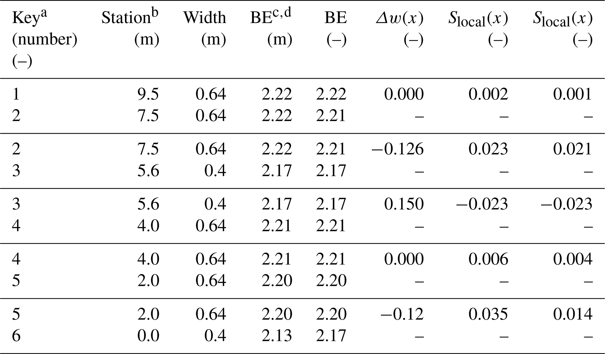
B1 Richards (1976), Fig. 3

Figure B1 Modified Fig. 3 of Richards (1976) showing the locations of channel width and elevation profile measurements indicated by the open circles. The width series is at the top of the image, and the elevation profile series is at the bottom. Values are in meters. Flow is right to left in the image.

Table B1 Measurement details for Fig. 3 of Richards (1976).

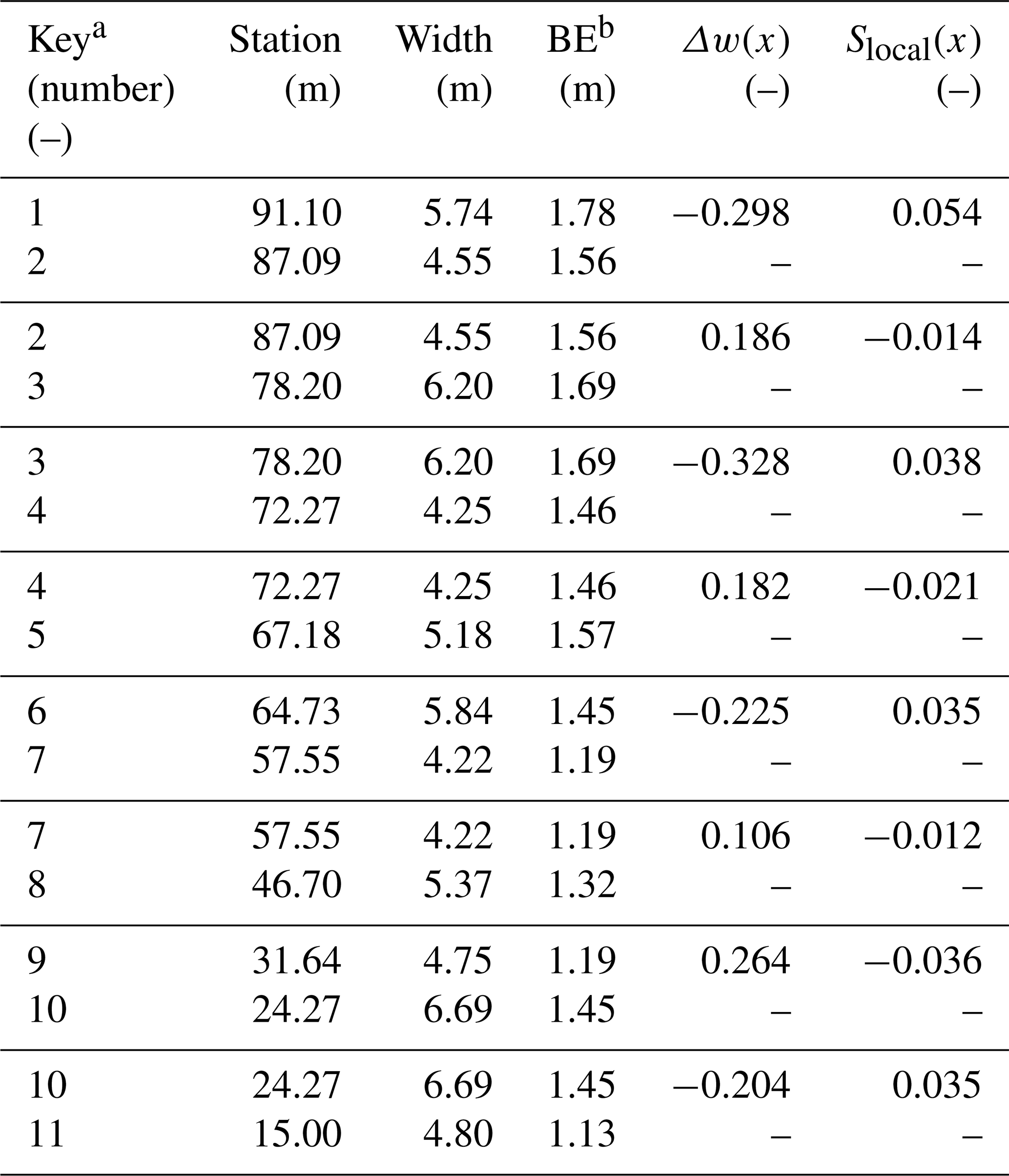
^a Key begins with the first measurement point at the upstream end of Fig. 1. ^b BE stands for bed elevation.

B2 Figure 4 of Richards (1976)

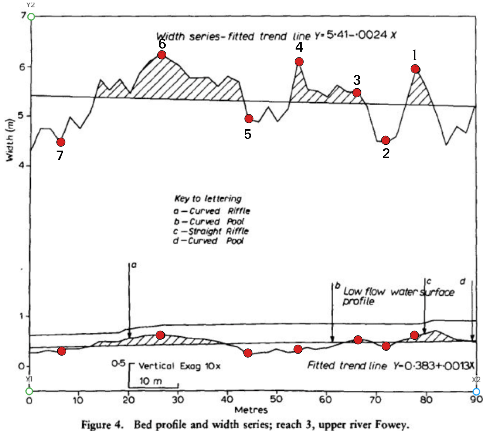
Figure B2 Modified Fig. 4 of Richards (1976) showing the locations of channel width and elevation profile measurements indicated by the open circles. The width series is at the top of the image and the elevation profile series is at the bottom. Values are in meters. Flow is right to left in the image.

Table B2 Measurement details for Fig. 4 of Richards (1976).

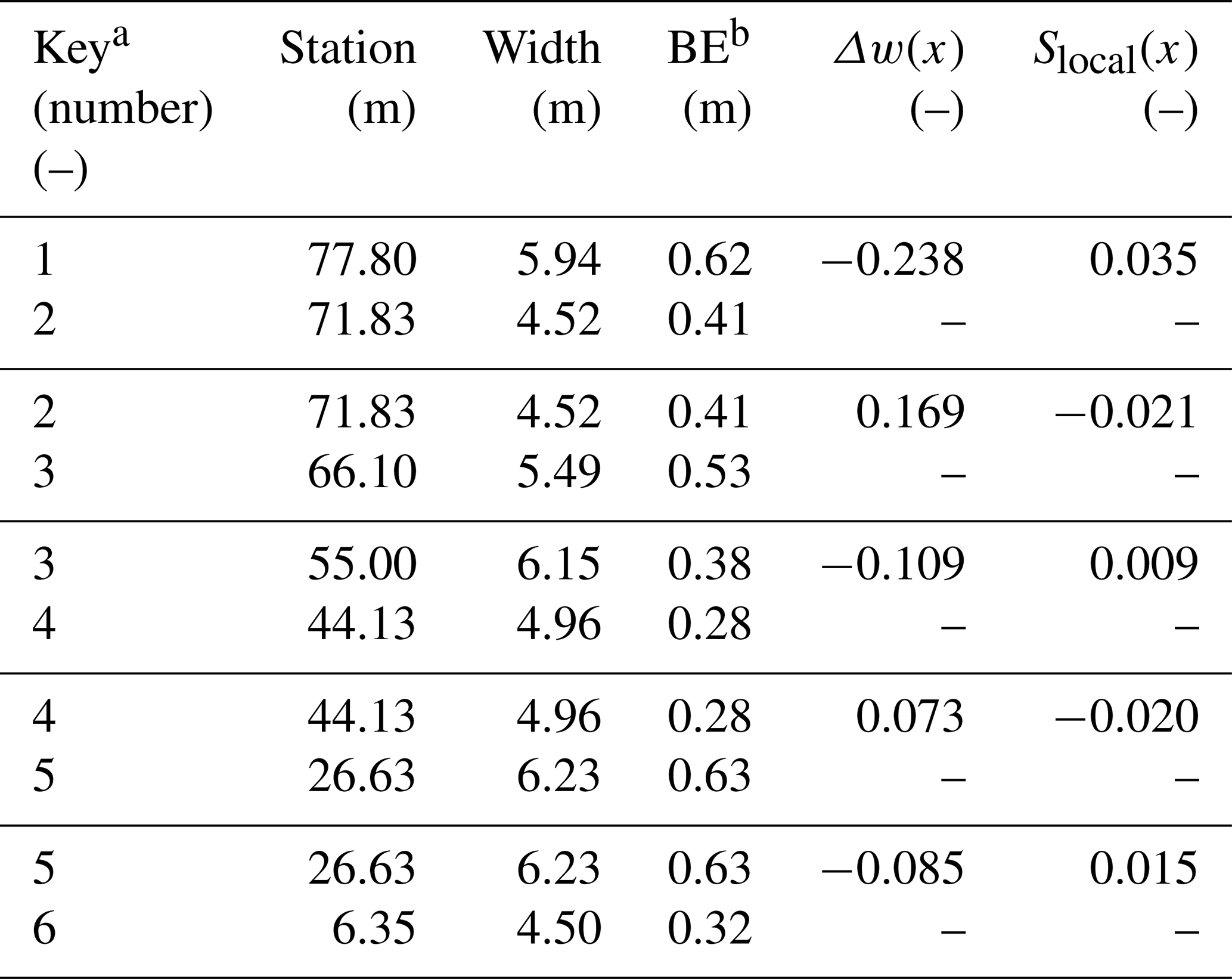
^a Key begins with the first measurement point at the upstream end of Fig. 3. ^b BE stands for bed elevation.

B3 Figures 3 and 4 of Cao et al. (2003)

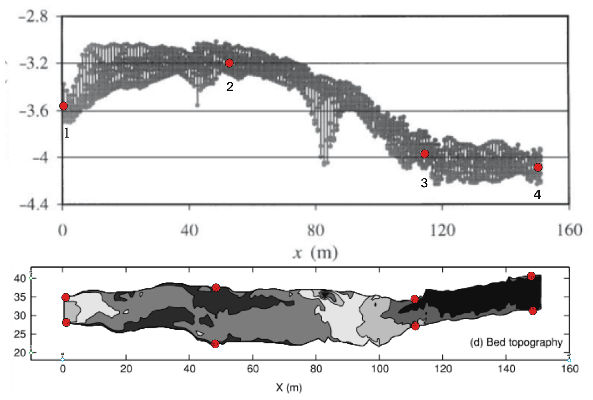
Figure B3 Modified Figs. 4 (top) and 3 (bottom) of Cao et al. (2003) showing the locations of channel width and elevation profile measurements indicated by the open circles. The bed elevation series is at the top of the image and the width series is at the bottom. Here channel width was measured as the distance in between the points at the two bounding edge positions at a given channel station. Units are meters. Flow is left to right in the image.

Table B3 Measurement details for Fig. 4 of Cao et al. (2003).

^a Key begins with the first measurement point at the upstream end of Fig. 6. ^b Channel stationing was flipped to have zero at the downstream end. ^c BE stands for bed elevation.

B4 Figure 5 of Brew et al. (2015)

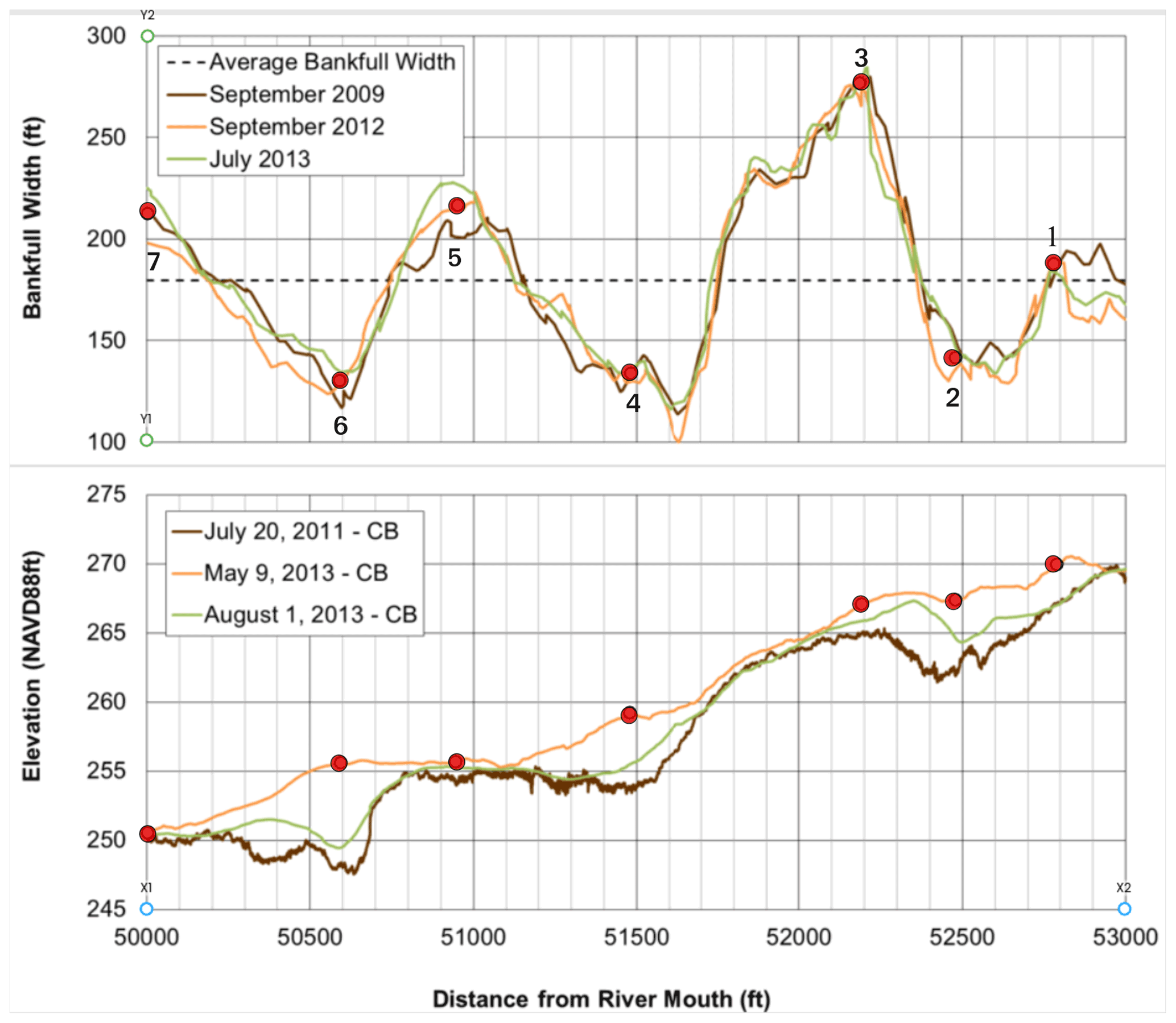
Figure B4 Modified Fig. 5 of Brew et al. (2015) showing the locations of channel width and elevation profile measurements indicated by the open circles. Width measurements are approximate averages of the three series shown. Elevation measurements were made for each profile by shifting the indicated points straight down to the next profile line below the top one (orange). Values are given in feet to remain consistent with the cited publication. To convert to SI units of meters multiply all values on the x and y axes by 0.3048. Flow is right to left in the image.

Table B4 Measurement details for Fig. 5 of Brew et al. (2015).

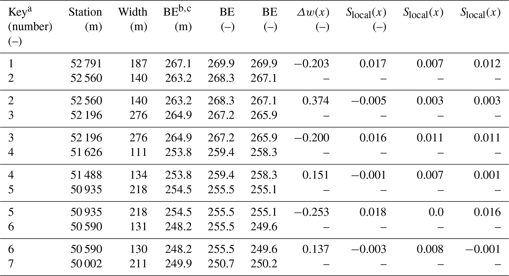
^a Key begins with the first measurement point at the upstream end of Fig. 4. ^b BE stands for bed elevation. ^c Bed elevation and S_local(x) ordered column-wise for July 2011, May 2013, and August 2013.

B5 Figure 3 of Vahidi et al. (2020)

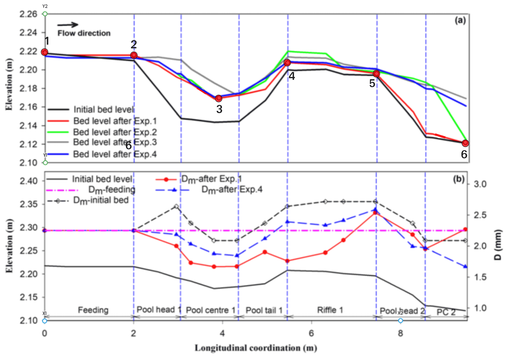
Figure B5 Modified Fig. 5 of Vahidi et al. (2020) showing the locations of channel width and elevation profile measurements indicated by the open circles. The elevation profile series is at the top of the image. Width measurements were taken from Fig. 1 of Vahidi et al. (2020). Elevation measurements were made for Experiments 1 and 4 by shifting the indicated points straight up to the Experiment 4 line where they do not overlap. Values are in meters. Flow is from left to right in the image.

Table B5 Measurement details for Fig. 5 of Vahidi et al. (2020).

^a Key begins with the first measurement point at the upstream end of Fig. 5. ^b Channel stationing was flipped to have zero at the downstream end. ^c BE stands for bed elevation. ^d Bed elevation and S_local(x) ordered column-wise: Experiment 1, Experiment 4.