Automated classification of seismic signals recorded on the Åknes rock slope, Western Norway, using a convolutional neural network

A convolutional neural network (CNN) was implemented to automatically classify 15 years of seismic signals recorded by an eight-geophone network installed around the back scarp of the Åknes rock slope in Norway. Eight event classes could be identified and are adapted from the typology proposed by Provost et al. (2018), of which five could be directly related to movements on the slope. Almost 60 000 events were classified automatically based on their spectrogram images. The performance of the classifier is estimated to be near 80 %. The statistical analysis of the results shows a strong seasonality of the microseismic activity at Åknes with an annual increase in springtime when snow melts and the temperature oscillates around the freezing point, mainly caused by events within classes of low-frequency slope quakes and tremors. The clear link between annual temperature variations and microseismic activity could be confirmed, supporting thawing and freezing processes as the origins. Other events such as high-frequency and successive slope quakes occur throughout the year and are potentially related to the steady creep of the sliding plane. The huge variability in the annual event number cannot be solely explained by average temperatures or varying detectability of the network. Groundwater recharge processes and their response to precipitation episodes are known to be a major factor of sliding at Åknes, but the relationship with microseismic activity is less obvious and could not be demonstrated.

1 Introduction

Norwegian landscapes have been shaped by deglaciation over thousands of years, creating very steep and mostly water-filled valleys, the fjords, over the western parts of the country. The steep flanks of the fjords are potentially unstable and their collapse poses a significant hazard. Most of these flanks are uninhabited and direct effects of a collapse would be rather limited. However, the mass sledging into the fjord can generate a local flood wave causing both infrastructure damage on shorelines and casualties. During the 20th century, 175 victims were reported in Norway due to such events (Kveldsvik, 2008). Worldwide, different factors contribute to the triggering of slides. For example, large earthquakes have the potential to trigger landslides or accelerate their sliding (Lacroix et al., 2015; Bontemps et al., 2020). Nevertheless, the most common causes for sliding are related to variations in the water content at depth both in terms of amount (e.g. infiltration following precipitation; Helmstetter and Garambois, 2010; Bontemps et al., 2020), pressure, and state (from solid during freezing to fluid during thawing; e.g. Krautblatter et al., 2013; Blikra and Christiansen, 2014). In addition to its sharp relief, Norway experiences cold winters and mild summers, especially in the north, which are favourable for the temporary extension of frozen ground in winter or the conservation of permafrost. A permafrost probability map for the steep slopes of Norway was established by Magnin et al. (2019). A total of 2 % of Norwegian slopes are believed to be covered with continuous permafrost, 9 % with discontinuous permafrost, and up to 20 % with sporadic permafrost. Elevations at which permafrost can be observed depend mainly on latitude and slope aspect; i.e. a high latitude and an exposure to the north would lower the limit (Magnin et al., 2019). In the same paper, it was additionally revealed that permafrost may occur on steep slopes at lower elevations than on less pronounced topography, particularly for north-facing flanks. Moreover, permafrost could have acted as a slope stabilizer over the past thousands of years. As a consequence of the current global warming, the permafrost cover shrinks, leading to rock slopes becoming more unstable (Hilger et al., 2021). Therefore, Norway may experience more catastrophic sliding events in the near future and a crucial aspect is to develop automatic monitoring systems on the slopes to mitigate the related risk.

Currently, only a few sites are instrumented in Norway (e.g. Blikra et al., 2005; Nordvik et al., 2010; Blikra and Christiansen, 2014; Böhme et al., 2013). The Åknes unstable rock slope, subject of the present work, started being heavily instrumented in 2004 (Nordvik et al., 2009) and is considered the best and most thoroughly monitored rock slope in Norway. As part of the monitoring system, seismic instruments were installed to passively record seismic activity on the slope. Because seismic sensors do not only record events related to the movements of the slope but also regional earthquakes and anthropogenic noise, it is important to be able to distinguish between different types of signals. The network was fully functional in 2007, and since then, around 60 000 events have been detected. The combination of this large number of data and the need for real-time implementation then required automation of the classification task.

In this paper, we will first present the Åknes site both in terms of geology and monitoring, with a particular focus on the seismic monitoring, and then describe the automatic classifier implementation. The statistical analysis of the results shows the implications in terms of slope monitoring, particularly with the aim of better understanding the processes at play.

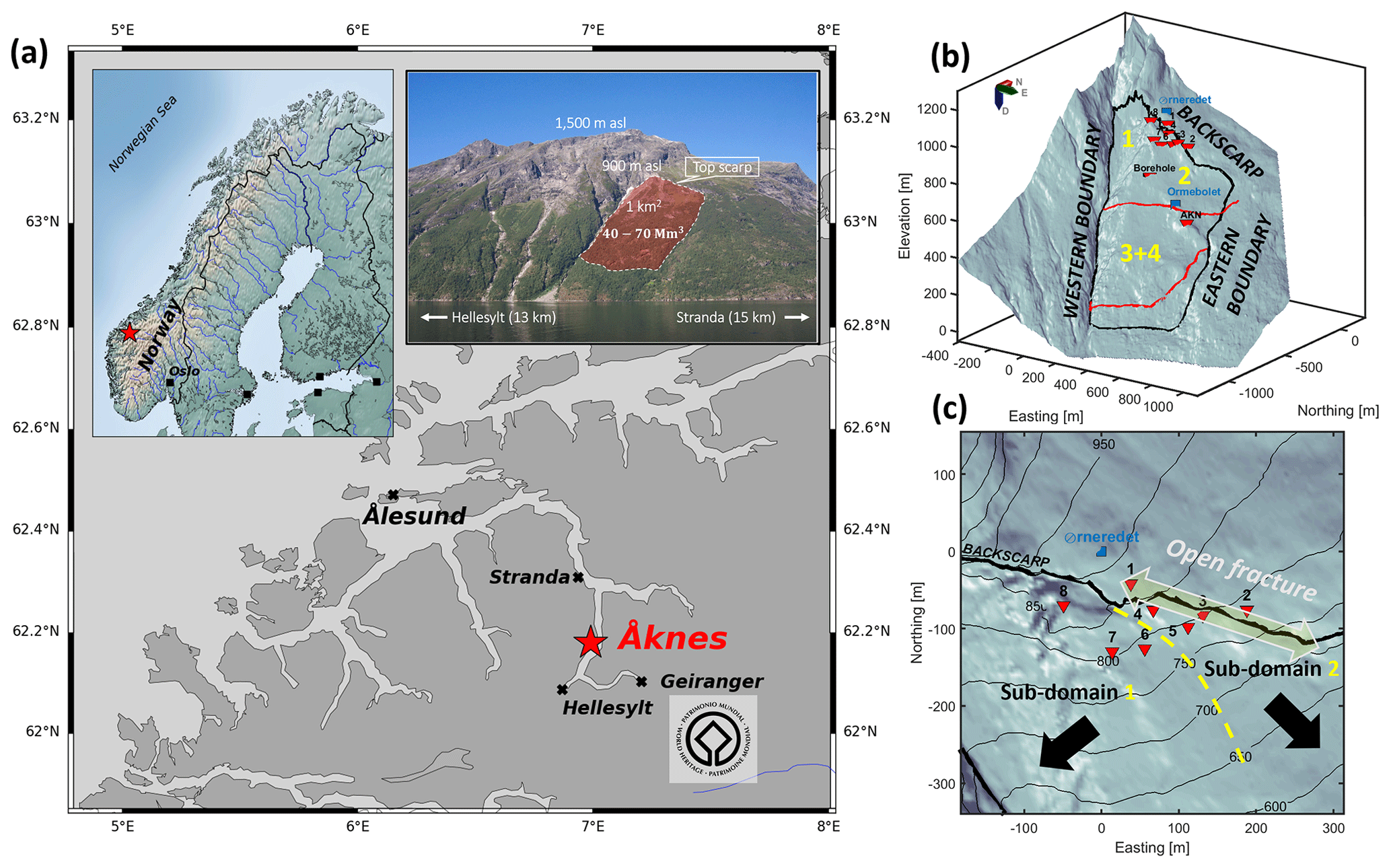
Figure 1 (a) Åknes rockslide location in Western Norway (red star). The photo at the top right shows the Åknes slope seen from the opposite side of the fjord (Roth and Blikra, 2010). The red shaded area represents the unstable area. Digital elevation model of the slope in 3D (b) and map view (c), zoomed to the top scarp, where the eight surface geophones are placed (red reversed triangles). The two main bunkers at the top and in the middle of the slope are displayed as blue squares. We use a local coordinate system centred on the upper bunker (Ørnereiret). In (b), the black contour delimits the whole area that could potentially collapse into the fjord. The red lines highlight two of the sliding planes. Sub-domains are indicated by yellow numbers. In (c), the back scarp splits the network in two, with geophones 1 and 2 placed on the stable ground behind the back scarp. The open fracture is highlighted by the yellow double arrow. The 50 m spaced elevation contours are also plotted. The two black arrows indicate the approximate displacement direction in sub-domains 1 and 2, and the dashed yellow curve marks the separation between the two sub-domains.

2 The Åknes unstable rock slope

2.1 Geology

The Åknes unstable rock slope (62^∘10.77^′ N, 6^∘59.45^′ E) is located in the municipality of Stranda in the Møre og Romsdal county in Western Norway (Fig. 1a). It overhangs the Sunnylvsfjord, which branches off to the Geiranger fjord in the south-east. This fjord became a World Heritage Site in 2005, attracting a growing number of tourists and cruise ships each year. The need for ensuring safety in the surroundings of this important touristic site partly explains why the Åknes slope received a great deal of attention. The slope faces south with a very steep topography from sea level to 1300 m altitude over a distance of about 1500 m (Ganerød et al., 2008). The rock formations consist of three main types of gneisses, the foliation of which is parallel or sub-parallel to the slope. The steep slope angle (30–35^∘) and the foliation constitute the two main geological factors for instability. The unstable part is delimited in the west by a NNW–SSE-striking and steeply dipping strike-slip fault resulting in a cliff of 10 to 40 m height (Fig. 1b). A NNE–SSW-striking and gently NW-dipping strike-slip fault forms the eastern boundary. The upper limit, the back scarp, is characterized on its western part by a cliff and graben, separating geophones 6, 7, and 8 from the others, and on its eastern side by an open fracture whose depth is difficult to estimate but is estimated to be about 60 m deep in the western part, reaching to somewhat shallower depth towards the east (Fig. 1c). Geological observations at the surface and investigations using different geophysical methods (including radar, refraction seismics, and resistivity profiles) led to the division of the unstable slope into four sub-domains (Ganerød et al., 2008), which – depending on the scenario – could collapse simultaneously or independently of each other. In the worst-case scenario, the total volume of unstable material was estimated to be more than 50×10⁶ m³ (Fig. 1b), which would result in a tsunami with up to 85 m run-up height at the nearby villages (Harbitz et al., 2014). Two sliding planes beneath the extensional upper sub-domains (1, 2) as well as beneath the lower compressional sub-domains were evidenced from surface observations (Fig. 1b, red lines).

2.2 Monitoring

The first evidence of movement at the Åknes rock slope was reported as early as 1964, when locals observed a widening of the upper crack (Grøneng et al., 2011). Today, the slope is continuously monitored by NVE (the Norwegian Water Resources and Energy Directorate) and is thoroughly equipped with numerous types of instruments. Displacement rates are measured by 5 extensometers within the upper crack, 2 lasers at the back scarp, 10 permanent GPS points and 30 prisms covering the whole slope (Pless et al., 2021). Displacement measurements were also regularly performed through field campaigns of remote-sensing techniques such as ground-based and satellite-based InSAR (interferometric synthetic-aperture radar; Kristensen et al., 2013; Bardi et al., 2016) and terrestrial laser scanning (TLS;  Oppikofer et al., 2009). Annual displacement rates of a few millimetres to up to 8 cm (Nordvik and Nyrnes, 2009) with an average of 1–2 cm yr⁻¹ were recorded (Ganerød et al., 2008). Larger displacements were observed in the upper part of the slope (sub-domains 1 and 2) compared to the lower part (sub-domains 3 and 4; Ganerød et al., 2008). Twelve boreholes were drilled and instrumented with inclinometers to monitor deformation as well as piezometers to survey groundwater level variations. Groundwater fluctuations are believed to be the main reason for the slope movement. Increases in the groundwater level are correlated with increases in measured displacement rates (Nordvik and Nyrnes, 2009; Grøneng et al., 2011). The data are not self-sufficient, though, and need to be integrated with models of groundwater recharge processes. Hence, many hydrogeological field campaigns were conducted in summertime to map the streams on the slope and collect geochemical and flow data to better characterize water movement (Sena and Braathen, 2021). Last, but not least, a meteorological station installed close to the upper bunker (blue square in Fig. 1b, c) measures the temperature, precipitation, wind speed, and snow cover.

As part of the monitoring system, seismic instruments were installed. Passive seismic monitoring has the advantage of continuously recording waves propagating within the ground either in the form of well-identified seismic events or as background noise. In terms of slope monitoring, an increase in the number of detected seismic events can indicate movements of and on the slope. The magnitude of such events may help characterize the type of slope movement; e.g. a few large events or many small events can result in the same amount of movement but caused by different processes. In addition, seismic events can be of various origins and they may be located at the surface or at depth, hence providing information about the rock properties in the subsurface. Therefore, many rockslides worldwide are continuously monitored seismically (e.g. Spillmann et al., 2007; Dammeier et al., 2011; Lacroix and Helmstetter, 2011; Gomberg et al., 2011; Tonnellier et al., 2013; Arosio et al., 2018; Vouillamoz et al., 2018). Seismic precursors to rock slides have been observed on different scales (Senfaute et al., 2009; Walter et al., 2012; Yamada et al., 2016; Poli, 2017; Schöpa et al., 2018; Butler, 2019; Zhang et al., 2019) and seismic records have been used to better understand rockfall dynamics as well (Hibert et al., 2017). In addition, an increasing number of studies leverages background seismic noise, which likewise contains valuable information (e.g. Colombero et al., 2018; Le Breton et al., 2021; Colombero et al., 2021; Kang et al., 2021). More precisely, tiny variations in seismic velocities can be measured by analysing long time series of ambient noise. It was observed that slope failures are preceded by an irreversible drop in velocity, which can be directly linked to a loss of rigidity of the material. More interestingly, reversible and seasonal changes are generally measured, giving an insight into the different, site-specific processes at play.

2.3 Seismic data

At Åknes, a small-scale seismic network composed of eight three-component geophones was set up in 2005 (Roth et al., 2006; Fischer et al., 2020) around the back scarp, which represents the most active zone, and has been continuously recording ground motion since 2006. The network total extent is 200 by 300 m. Seismic data are recorded in triggered mode with a low threshold to include as many events as possible. In the case of a trigger, 16 s long files, sampled at 1000 Hz, are transferred to NORSAR in near real time, where a more selective automatic STA/LTA (short-term average over long-term average) detection (Withers et al., 1998) is performed. In 2009, the seismic instrumentation was supplemented by a broadband seismometer (AKN) in the central, more stable part of the slope for continuous data recording. This station, operated by NORSAR, provides data to the Norwegian National Seismic Network (NNSN) and the European Integrated Data Archive (EIDA) and contributes to the regional and teleseismic earthquake monitoring. So far, it has not been used for slope monitoring in a systematic manner. Lastly, in 2017, a string of eight geophones was installed in a borehole in the upper part of the slope, just above one of the sliding planes (Fig. 1b). The present paper will focus exclusively on the data registered on the surface geophone network. In Sect. 5, we will discuss how the other available data streams may complement this work in the future.

It must be noted that network maintenance is challenging due to the harsh conditions and the limited fieldwork season. In particular, cables between surface geophones and digitizer are the weakest links and are regularly sheared by either rockfalls or snow avalanches. For example, geophones 6, 7, and 8 in the western part of the slope are separated from the others by a gully, which is particularly prone to rockfalls, while geophone 2, in the eastern part of the slope, is placed in a snow avalanche corridor. As a consequence, there are variations in detectability inherent in the dataset.

Rockslides can generate various types of seismic signals which have been analysed in several detailed studies at different sites (e.g. Helmstetter and Garambois, 2010; Occhiena et al., 2012; Tonnellier et al., 2013; Vouillamoz et al., 2018). Provost et al. (2018) brought together data recorded on different landslides (including Åknes) and proposed a standardized typology reflecting the diversity of these signals, composed of three main classes (slope quakes, rockfalls, and granular flows) subdivided into several subclasses. This typology must be adapted to site-specific characteristics, being aware that the network layout, the type of sensors, and the acquisition parameters have an effect on records, data analysis, and subsequently typology. Moreover, even though different types of signals are observed at various sites, their physical origins are still relatively unknown. For example, the frequency content of a recorded signal depends on the distance from the source to the recording station, especially if the medium is highly heterogeneous, dispersive, or attenuative. Thus, records from a single event may have different seismic signatures at different stations. Likewise, two events having a similar source mechanism but occurring at different locations may display completely different waveforms. Event locations can help discriminate between source and path effects. However, accurately locating events on rockslides to highlight structures at depth is usually far from being straightforward. At Åknes, the medium is highly fractured and highly attenuative; hence, an adequate velocity model is difficult to establish and seismic phases are not always easily identifiable on the waveforms. Several attempts have been made to locate the events; for example, Fischer et al. (2020) applied a back-propagation approach limited by the use of only a homogeneous velocity model and by constraining the locations to the surface. In the same paper, seismic events were divided into four categories (microseismic events, rockfalls, distant events, and noise), but this work represented a feasibility study and was not systematically implemented as part of the automatic monitoring system.

The goal of the present work is (1) to identify the different signals recorded at Åknes, (2) to establish an automatic classifier, (3) to integrate it in the current processing routines in a way in which non-seismologists can exploit the catalogue of detected events without having to interpret the waveforms, and (4) to discuss the classification of events in light of the processes involved in the slope movement. For that purpose, a large amount of waveforms was visually inspected and event classes were manually assigned following a modification of the typology proposed by Provost et al. (2018). In the next paragraphs, various observed signals are described.

3 Description of observed seismic signals

The first main class of seismic events is called slope quakes. This terminology was introduced in order to avoid the wide variety of terms that can be found in the literature (microquakes, quakes, microseismic events, and so forth). This class is further subdivided into simple and complex slope quakes. Simple slope quakes correspond to events that are believed to be associated with either the fracturing or the sliding of the slope. Based on their frequency content, several mechanisms may be hypothesized (Provost et al., 2018). Complex slope quakes encompass signals that are believed to be directly associated with phenomena affecting the slope stability at depth, such as tremors, but their origin is more speculative and, so far, not as well understood.

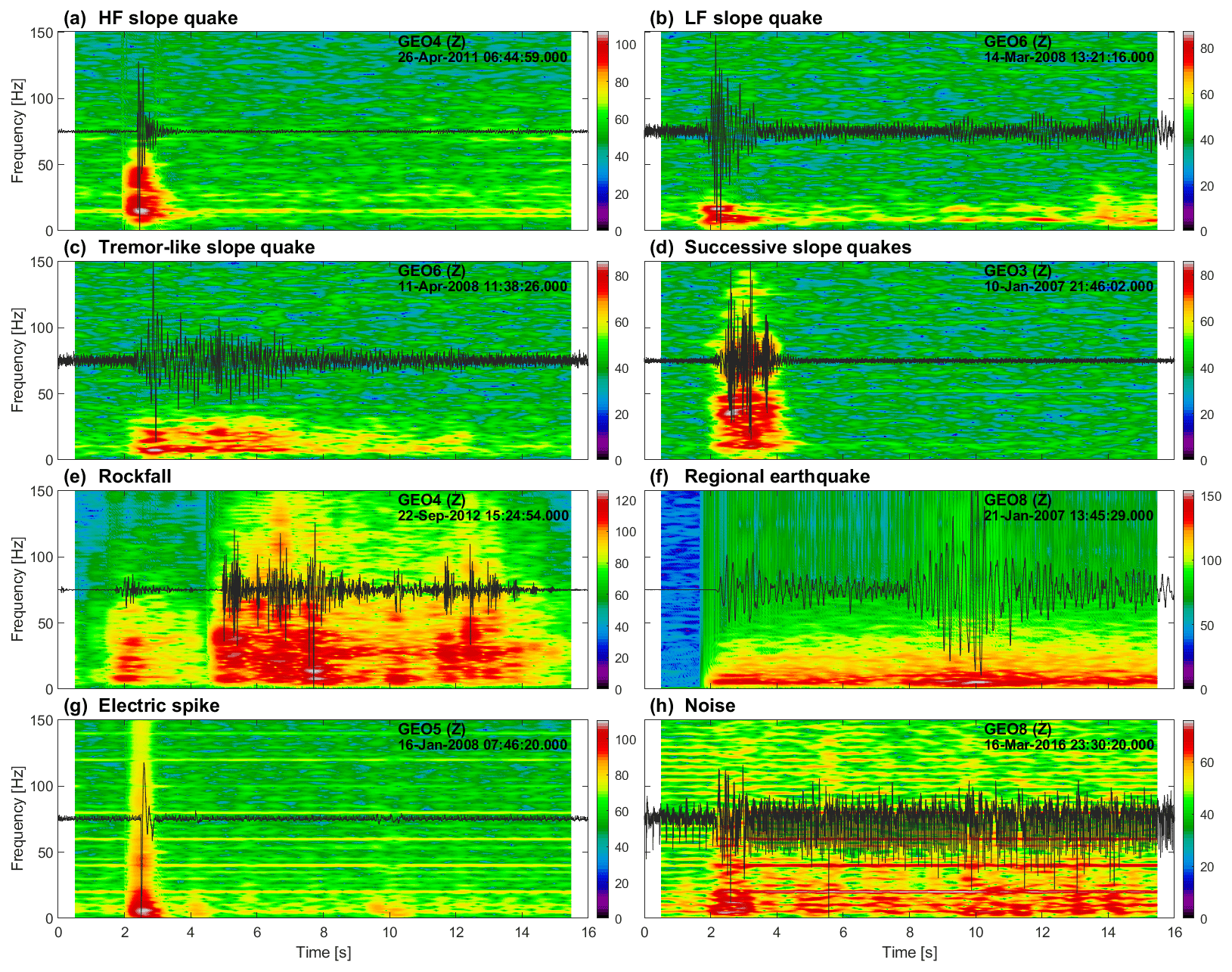
Figure 2 Spectrograms and normalized waveforms of the maximum-amplitude record of signals representative of each class: (a) HF slope quake, (b) LF slope quake, (c) tremor, (d) successive slope quakes, (e) rockfall, (f) regional earthquake, (g) spike, and (h) noise. Note that colour scales are in a logarithmic scale [dB] and not normalized. Frequencies are only shown up to 150 Hz. In (f), both the P- and S-wave arrivals are visible at ca. 2 and 8 s, respectively. Vertical component waveforms of the example events recorded at all geophones are displayed in the Appendix (Figs. B1 to B8).

At the Åknes site, high-frequency (HF) and low-frequency (LF) simple slope quakes are observed as well as tremors. HF slope quakes are impulsive and short-duration events, usually < 2 s (Fig. 2a). They contain energy at frequencies above 40 Hz and regularly comprise frequencies of 80 Hz or more. Differences in the higher-frequency content may be an effect of the distance of the geophones to the source; therefore HF events are grouped into a single class. While lasting approximately as long as HF slope quakes, LF slope quakes feature emergent onsets hampering the identification of the signal start, and their energy is mostly concentrated in frequencies below 25 Hz (Fig. 2b). Usually, their maximum amplitude is much lower. Tremors have similar characteristics to LF slope quakes but a longer duration (> 4–6 s, Fig. 2c). They partly exhibit a large portion of harmonic signals. Lastly, we defined a class of successive HF slope quakes (Fig. 2d). They present roughly similar characteristics to HF slope quakes but possess a longer duration (2 to 4 s) and consist of several bursts of energy (up to four).

In addition to events taking place at depth, surface processes caused by the slope steepness and instability such as rockfalls, snow avalanches, and granular flows are recorded. Due to the file length limitation to 16 s and detection settings, snow avalanches are very often either not detected or difficult to classify. Therefore, we do not have a dedicated class in the present classifier, and the corresponding signals potentially are classified as noise (see Sect. 5). Rockfalls, on the other hand, can exhibit a wide range of waveforms and can be associated with different processes, e.g. a single rock splitting and falling down, a rock bouncing repeatedly, or a larger rock block collapsing. In general, rockfalls are characterized by emergent signals of longer duration than simple slope quakes (> 2 s). They cover a large frequency bandwidth, reaching up to 150 Hz or more, and their waveforms display several bursts of energy (Fig. 2e) as well as a high variability across the seismic network (Fig. B5).

Seismic instruments also record signals that occur farther away (e.g. regional earthquakes) and electric noise, mostly as spikes. Although not relevant to the slope monitoring, they need to be classified in order to be removed. Thus, spikes are defined as short, narrow, and high-amplitude signals (Fig. 2g), whereas regional earthquake durations always exceed the file length of 16 s (Fig. 2f). However, a pitfall for regional earthquakes is that, depending on the source location, the S wave may not be visible in the records. Therefore, phenomena of longer duration such as snow avalanches or granular flows may be regarded by the classifier as regional earthquakes.

Lastly, we defined a “noise” class, corresponding to all signals that do not exhibit distinct features allowing them to be classified as any of the previously described classes (Fig. 2h). In practice, this class only contains few events, since the STA/LTA detector is sufficiently restrictive to discard noisy signals.

The main characteristics and the hypothesized mechanical processes of each event class are summarized in Table 1, while their relationship to the slope geology is represented schematically in Fig. 3.

Table 1 Summary of the seismic event classes identified at Åknes. Asterisks (^*) indicate events that occur directly on the slope and are therefore relevant and meaningful for the monitoring. Hypotheses on the physical processes causing the events are provided, inferred both from the literature and the observations at Åknes developed in Sect. 5. N_tr and N_t are the number of events constituting the training and test sets, respectively. Probability density functions of the main signal characteristics are shown in Fig. B18 in the Appendix.

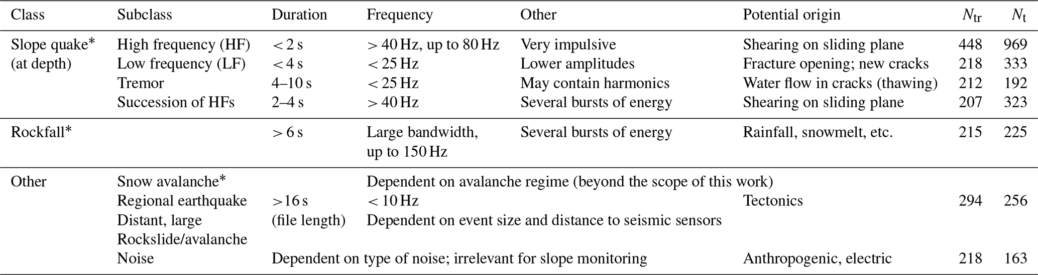
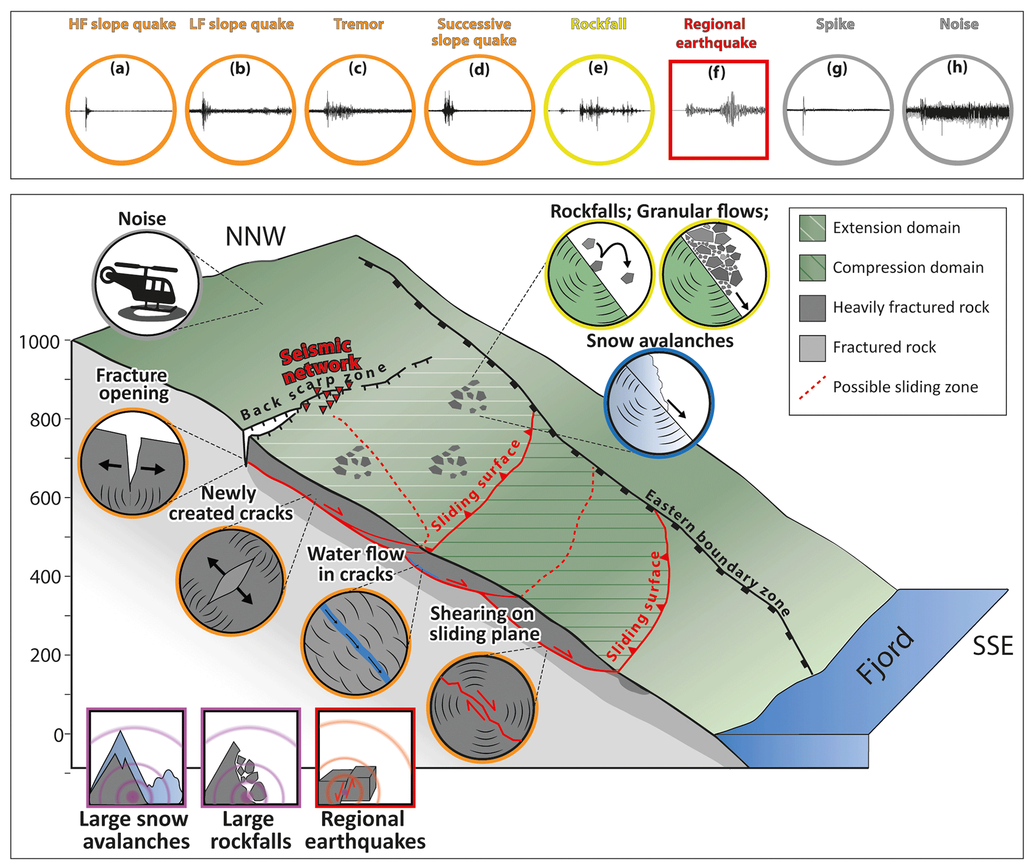
Figure 3 Sketch of the Åknes rock slope featuring local and distant natural phenomena generating seismic signals (see Table 1). Adapted from Fig. 10 in Ganerød et al. (2008) and Fig. 1 in Provost et al. (2018). Waveforms at the top are the same as the ones in Fig. 2.

4 Classification

4.1 Background

Automated classification of seismic signals started as early as the 1990s, when Dowla et al. (1990) discriminated natural earthquakes from nuclear explosions. Later on, it was successfully applied and developed in the field of volcano seismology (e.g. Falsaperla et al., 1996; Ohrnberger, 2001; Masotti et al., 2006; Curilem et al., 2009; Langet, 2014; Maggi et al., 2017; Malfante et al., 2018) and recently on rockslides (e.g. Hammer et al., 2013; Provost et al., 2017; Feng et al., 2020; Lin et al., 2020). Amongst the most commonly used methods are neural networks (NNs), hidden Markov models (HMMs), support vector machines (SVMs), and random forest (RF).

Classification is a supervised learning problem. This implies that a set of well-known data was labelled and used to train the machine learning algorithm. Building a good training set is crucial, since in the case of supervised learning, the system is not able to learn anything new by itself: a signal will always be divided into one of the pre-defined classes. A training set should therefore be representative of the data and provide an exhaustive sampling in terms of (1) classes present in the data and (2) data quality. The representativeness is important due to the trade-off between the classifier generalization and its precision, the aim being to maximize the number of correctly classified events, while minimizing the number of incorrect classifications for all classes.

For the Åknes dataset, events were classified by visual inspection of a large number of waveforms recorded in different years. Except for the sparsely populated noise class (only 10 events), each class contains approximately 200 events. The distribution of classes across the training set is recognizable in Fig. B11a in the Appendix and numbers are given in Table 1. Most classes constitute around 12 % of the training set. The class of HF slope quakes is twice as large in size (ca. 24 %) as it appears to be the dominating event class in the whole dataset. The regional earthquake class contains slightly more events (16 %) and was cross-checked with a reviewed seismic bulletin (NORSAR, 1971) to ensure the proper labelling of corresponding events.

4.2 Convolutional neural network

Machine learning methods have developed quickly during the past few years. Breakthroughs have occurred not only due to the development of new conceptual approaches but also because of substantial improvements in hardware and computational capacity, which allow dealing with a much larger number of data. In particular, deep learning methods are now able to classify images (Hinton et al., 2006) by creating a model not only for conditional probabilities P(Y|X) (i.e. probability of an event belonging to class Y knowing its set of features X) but for joint probabilities P(X,Y) (i.e. the event belongs to the class Y maximizing the conditional probability P(Y|X) given its image X).

Traditionally, in machine learning methods such as SVM or RF, the input data are discretized into feature vectors for which the features are extracted from the raw data with the aim to offer a best possible description. Due to the complexity of seismic waveforms, these features should describe the signals in the time domain in terms of duration, shape (e.g. number of peaks, peakedness), in the frequency domain (e.g. predominant and central frequencies, spectrum bandwidth) and in the cepstral domain (the cepstral domain results from the inverse Fourier transform of the logarithm of a Fourier spectrum; e.g. Malfante et al., 2018). The number of features effectively used by the system may be reduced by removing correlated features and performing principal component analysis (PCA). Feature-based methods have the advantage that they are easier to understand in the sense that features that are the most discriminant for each event class can be identified. However, their main drawback is that these features must be pre-defined manually, and selecting them may be rather subjective.

Waveform complexity may act as an obstacle to classification; i.e. the classifier will be difficult to generalize and will have a tendency to over-fitting, resulting in each individual event defining a class if the waveforms are not sufficiently similar. Spectrograms, on the other hand, constitute a simplified representation of waveforms in the time–frequency domain. They contain the same information but include a temporal reference in addition. Discretized features can also be extracted from spectrograms (e.g. distance between the maximum and mean frequencies; see Provost et al., 2017; Hibert et al., 2017; Wenner et al., 2021). However, defining such features can be avoided as spectrograms can already be seen as matrices of features that are not defined explicitly. For example, the duration information corresponds to the time span in which most of the energy is concentrated, instead of being defined by a scalar value expressed in seconds. Such information matrices can be processed as images by convolutional neural networks (CNNs). Filters in the CNN's convolutional layers act as features; the more layers, the more filters are applied and the more features are extracted. The filter parameters are learnt during the training process. Pooling and resampling layers do not learn new parameters but decrease or increase the number of features. They may help in the identification of dominant features. The classification itself is carried out by a fully connected layer. Convolution being a linear operation, convolutional layers must be accompanied by an activation function for the system to learn non-linear features. There are many different activation functions available; for example, ReLU (rectified linear unit) is widely used and consists in keeping only positive values after the convolution operation, while negative values are replaced by zeros. The architecture of the CNN, i.e. the number of layers, their order, the type of activation functions, etc., offers great flexibility, and choices may affect the classification results. Still, well-known architectures have proved to be successful in a wide range of applications (e.g. LeNet-5, AlexNet, ResNet).

In the Åknes network, each event is recorded by eight geophones on three channels, i.e. on 24 traces in total. Depending on the source location and its distance to each geophone, wave onsets are not simultaneous across the network and the different ray paths through a very heterogeneous medium distort the waveforms recorded at each geophone. However, since inter-station distances are short, differences in travel times are expected to be small. Therefore, we simplify the information by (1) computing individual spectrograms for all channels and (2) stacking them all together, resulting in a single image. Note that we only stack spectrograms for geophones that detected the event and remove low-quality traces. A trace is regarded as low-quality if its signal-to-noise ratio (SNR) is much lower than the SNR of the other traces, i.e. if ${\mathrm{SNR}}_{\mathrm{tr},\mathrm{norm}}<\mathrm{0.7}\cdot \frac{\stackrel{\mathrm{‾}}{\mathrm{SNR}}-{\mathit{\sigma }}_{\mathrm{SNR}}}{max\left(\mathrm{SNR}\right)}$, where SNR_tr,norm is the normalized SNR of the trace, $\stackrel{\mathrm{‾}}{\mathrm{SNR}}$ is the average SNR over all traces, and σ_SNR is the standard deviation. The factor 0.7 was finally chosen after testing on several data. In the end, this implies that the number of employed traces in each stack differs between events.

Practically, processing was implemented using the PyTorch python package (Paszke et al., 2019). We tested several CNN architectures (Silverberg, 2020) and chose the AlexNet architecture (Krizhevsky et al., 2017). In this pre-trained network, the RGB spectrogram images must have a fixed size [l, m, n], where l is the number of channels (three for RGB) and m and n are the height and width of the image, respectively. We computed spectrograms for the whole file length (16 s) using a 1 s long sliding window with a 95 % overlap. We truncated the spectrograms to 150 Hz, since only few events contain frequencies exceeding this value. After performance tests, the “afmhot” matplotlib sequential colour map was used to produce the spectrogram plot before its conversion to an RGB image of the size (3, 224, 224). The RGB values ranging from 0 to 255 are normalized for each channel. The best-performing optimizer as well as other determinant parameters for the CNN, such as the learning rate, were determined in advance by both grid search and cross-validation approaches. Finally, once the set of parameters yielding the best performance was found, the training of the final CNN was carried out on the entire training set.

4.3 Near real-time implementation

The supervised automatic classifier was implemented in near real time. For each newly detected event, spectrograms are extracted, stacked, and fed into the classifier. The resulting class is included in the catalogue of detections, a figure is produced (Fig. 4), and both are published on a dedicated web page (NORSAR, 2022) with a 10 to 15 min delay. Such figures are useful to visualize the event. In addition, the classifier returns probabilities, indicating the confidence with which the event was classified and, in the case of the event fitting multiple classes, the proportions with which these classes overlap. In Fig. 4, we show the example of an HF slope quake classified with a probability of 100 %.

Figure 4 Example of an event classified as a high-frequency (HF) slope quake by the automatic classifier. In (a), waveforms are shown for each component. Grey colour indicates geophones not contributing to the stack. Bold red text highlights the trace with maximum amplitude. The bottom trace represents the envelope stack of the traces with detection (black traces only). In (b), the spectrogram resulting from the stack of individual spectrograms computed for each channel is plotted employing the colour scale used in the CNN. In (c), the power spectral density (PSD) of the trace featuring the maximum amplitude is illustrated. Finally, in (d), the bar displays the classification probability.

In addition, the automatic classifier was also applied to the database of past events. Note that we excluded the year 2006, since the recording system was still in its test phase, and different sampling rates and file durations were used. Hence, the catalogue starts in 2007. Until the end of the year 2021, a total of 59 608 events were classified.

4.4 Results

In this section, we present the results from the classification process and attempt to interpret the outcome for the purpose of slope monitoring. A total of 20 % of the automatically classified events are not related to movements of the slope and represent regional earthquakes, electric spikes, and noise (Fig. B12). Note that in compliance with the training set, the noise class is almost non-existent. Of the remaining 80 % of events, 75 % correspond to slope quakes. Of those, HF slope quakes are largely predominant (38 %).

Since events are also classified manually on a daily basis by visually scanning waveforms and spectrograms, we established a test set consisting of 2554 events which are all different from the events contained in the training set. This test set is used to evaluate the performance of the CNN classifier in the confusion matrix in Fig. 5.

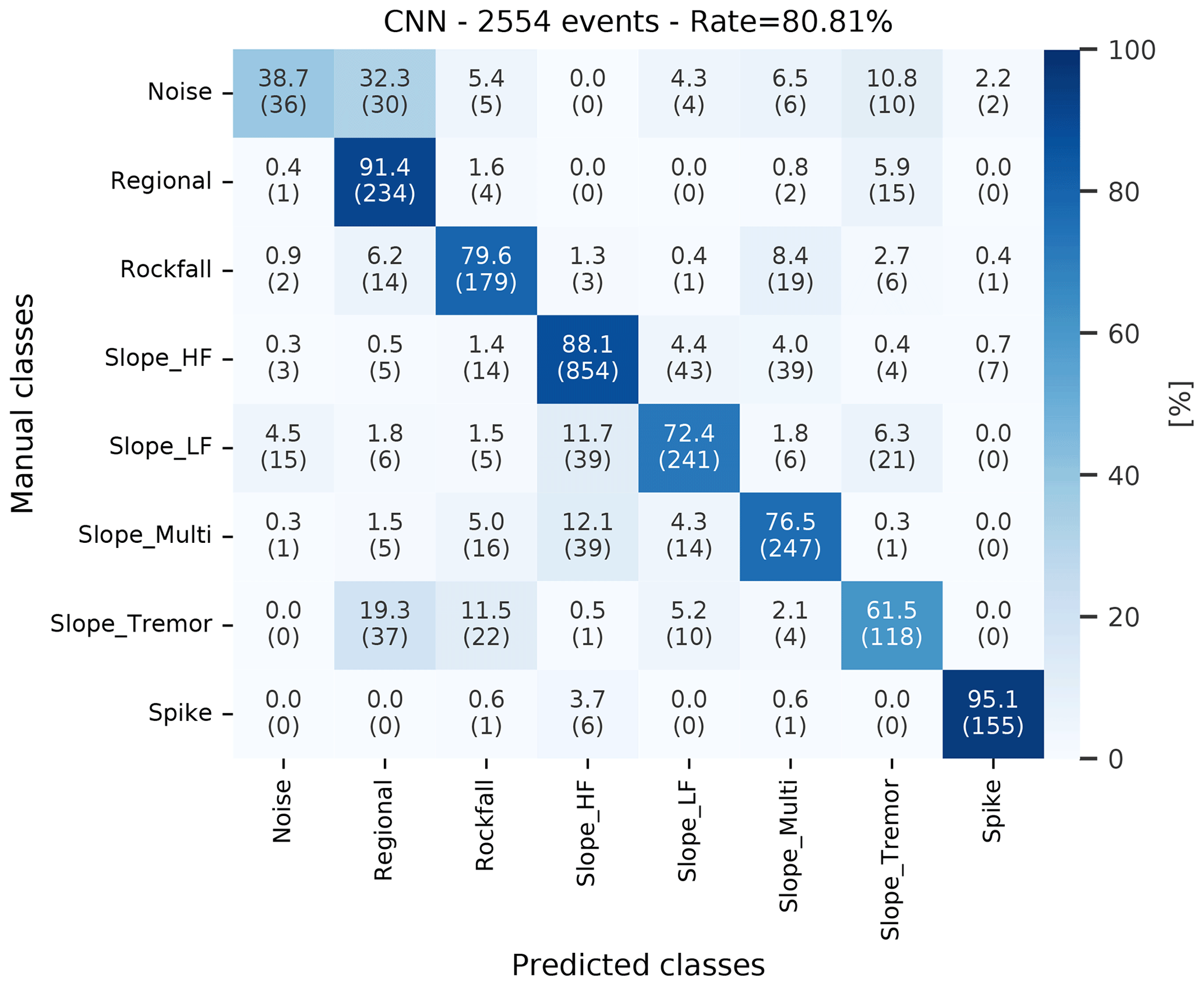
Figure 5 Confusion matrix comparing the results of manual and automatic classification for the test dataset. The matrix is colour-coded by percentage rates. Numbers in brackets indicate the absolute number of events in each class.

The distribution of manually attributed classes within the test set is shown in Fig. B11b and Table 1. We assume it to be representative of the whole dataset (Fig. B12). It is worthwhile noting that despite clearly defined characteristics, manual labelling is not straightforward for most of the events. Thus, manually defined classes should not be used as absolute ground truth and results should be interpreted with caution.

The CNN's overall success rate is good (slightly above 80 %) in spite of large discrepancies in success between classes (Fig. 5). Spikes are generally well identified as are 79 % of rockfalls. HF slope quakes are identified with a rate close to 88 %, whereas the LF slope quakes reach 72 %. More than 75 % of successive slope quakes are properly classified. Tremors constitute the event class that apparently is most difficult to classify with a success rate of only 61.5 %. This is not surprising, since the characteristics of this class are less clearly defined. Mostly, tremors are confused with regional earthquakes (19 %) and rockfalls (11.5 %). Finally, less than half of the signals corresponding to noise are properly recognized by the CNN. This is expected, since noise examples are severely underrepresented in the training set; instead the system tends to classify noise as regional earthquakes (32 %). The classifier has a tendency to classify more regional earthquakes and HF slope quakes than suggested by the manual classification; hence higher classification rates are reached for these classes.

To summarize, Fig. 5 shows that the classifier is able to properly discriminate between events that do not occur on the slope, with the possible exception of noise. However, the number of noise records is only marginal and will not affect the interpretation of the results. Events occurring on the slope reach classification rates of 75 % on average. However, due to the complexity of manual classification and the overlap between classes, those rates are considered satisfactory. The automatic processing results are more homogeneous and consistent than the manual ones.

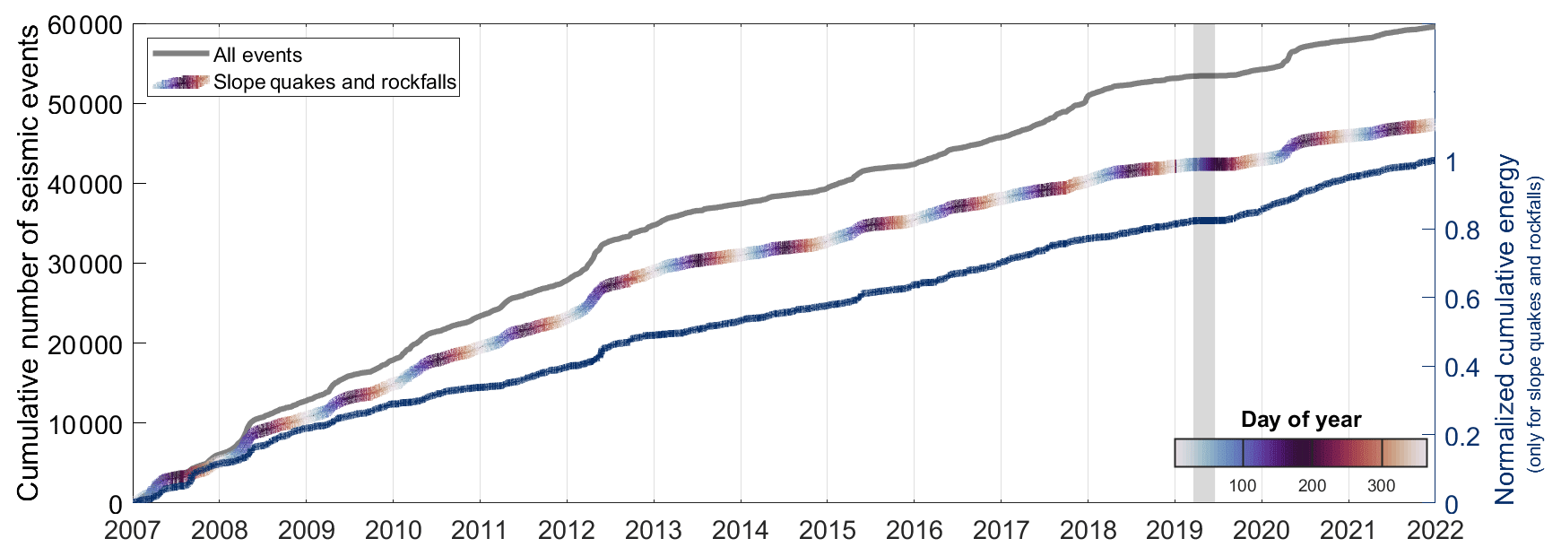
Figure 6 Cumulative number of seismic events and energy over time. Left axis: cumulative number of events including all detections (grey line) and restricted to events occurring on the slope (coloured line). The colour code highlights the seasonality. Right axis: normalized cumulative energy (dark blue line). The time range in 2019 shaded in grey corresponds to a period when the system was down and no data could be collected.

5 Discussion

The initial motivation for building a classifier was to better characterize seismic events recorded at the Åknes site. Although the number of detections provides information on the seismic activity rates over time, it does not allow us to discriminate between different mechanisms at play and may potentially be biased by including signals that are not linked to the slope. This is illustrated in Fig. 6 where the number of considered events drops to 47 561 after regional events, spikes, and noise are removed, thus comprising approximately 80 % of detections. Note that for this part of the interpretation only, the automatically generated catalogue was revised semi-manually to delete records of electric spikes erroneously classified as events, based on their maximum amplitude. The trend of the cumulative number-of-events curve, however, is not drastically different once these signals are removed (Fig. 6). In general, we observe a deceleration of the seismic activity since mid-2012 and regular inflections in the first half of each year, corresponding to an increase in seismic activity. In addition, Fig. 6 shows the cumulative energy of these local events in terms of squared amplitude used as a proxy for magnitude. Together with the cumulative number of events, it indicates whether the release of seismic energy was due to a few larger or multiple smaller events occurring within a short period of time. No particular episodes of higher-amplitude events emerge, suggesting that the energy is generated by small but numerous and regular seismic events.

Figure 7 Seasonality of events and temperature per month for 15 years of data (2007–2021). Left axis: number of events. Bars are subdivided into event classes; noise records are not visible, since they are sparse. Top right axis: average temperature (black line) including standard deviation (grey shade). Solid and dashed horizontal grey lines indicate temperatures of 0 and +4 ^∘C, respectively.

In the previous work by Fischer et al. (2020) analysing the same dataset for the time period 2006–2013, a seasonality of seismic activity was observed and a clear correlation with temperature variations was demonstrated. Both this study and the work by Grøneng et al. (2011) using displacement data showed that there is an acceleration of the sliding during spring which could be attributed to snowmelt. Indeed, by melting, the snow facilitates the infiltration of water into the fractures and towards the sliding plane, in turn increasing the pore pressure and reducing the friction and ultimately allowing for more sliding. In the following, we compare the catalogue of microseismicity with available meteorological data and expand the analysis further by adding the information on event types provided by the automatic classifier in order to identify which types of events are more related to meteorological conditions. Throughout a typical year, a significant increase in activity is observed in spring (from March to May), while summer months (June to September) are quieter (Fig. 7). There is also a gradual increase in seismic activity from October to February. This variation can be attributed to climatic conditions with temperatures below 4 ^∘C being reached regularly as early as in October. Temperatures are usually sub-zero from mid-November until the end of March. The transition to temperatures above zero occurs in April, and generally, temperatures exceed 4 ^∘C by the end of May. Liquid water has a density varying with temperature. Most notably, under normal atmospheric pressure conditions, its highest density is reached at a temperature of 4 ^∘C, while water turns into solid ice at temperatures of 0 ^∘C or below. Ice is thus less dense than liquid water, which means its volume grows. If the cracks in the rocks are filled with water and the temperature is oscillating between 0 and 4 ^∘C as observed from March to May, the variations in water density lead to seismic signals, which can be attributed to either (1) water state changes corresponding to freezing and thawing in water-filled micro-cracks, (2) the creation of new cracks, or (3) both. These explanations are in good agreement with the hypothesized mechanisms for the class of LF slope quakes and, interestingly, their number increases in spring (Fig. 7) while decreasing from June to October. Relative variations in the number of events are displayed in Fig. B13 in the Appendix and show that in addition to LF slope quakes, tremors, rockfalls, and, more surprisingly, regional earthquakes are also more numerous in spring. Rockfalls are more frequent in late summer and the beginning of autumn as well.

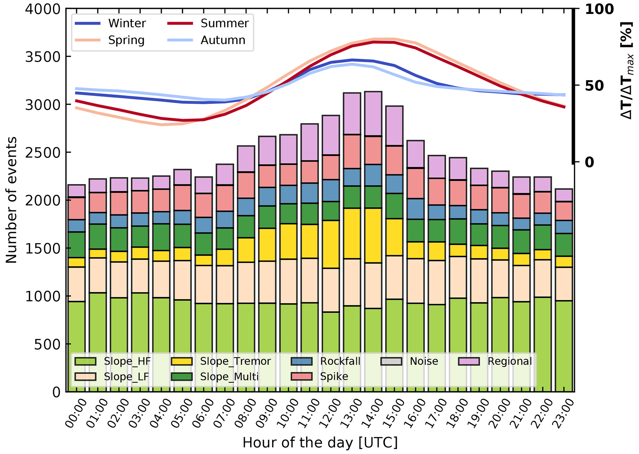
Figure 8 Distribution of detected events over hours of the day for 15 years of data (2007–2021). Left axis: number of events. Bars are subdivided into event classes; see legend of Fig. 7 for explanation. Top right axis: relative variations in temperature ($\mathrm{\Delta }T/\mathrm{\Delta }{T}_{\max }$) throughout the day, subdivided into seasons. For details, see Fig. C1.

Temperature appears to be a predominant factor influencing the microseismic activity on the slope (Fig. 7). This is also evident in daily data (Fig. 8) where we observe slightly more activity during the daytime (from ca. 08:00 to 16:00). This could indicate a potential contamination by anthropogenic noise; however, the Åknes site is remote, only accessible by helicopter, and therefore protected from such sources of noise. All human activities on the slope related to research and monitoring cease from the end of October to at least the end of April due to weather conditions prohibiting fieldwork. Moreover, Fig. 8 reveals that all classes of events, except tremors, occur in relatively constant ratios independently of the hour of the day. Since tremors are rarely observed in summertime (Fig. 7), an anthropogenic origin is improbable. Our observations show that tremors are mostly recorded during the snowmelt season and during the daytime. The curves of relative temperature variations clearly indicate that daily variations are larger in spring and summer compared to autumn and winter (Fig. 8). This is expected, since at the latitude of Åknes, the daylight period is as short as 5 h in winter. In Fig. C1 in the Appendix, we show both absolute temperatures and their relative variations for each month of the year. On the whole, those observations strengthen and confirm the thawing–freezing cycles as the leading cause of tremors. Although LF slope quakes are more numerous in spring (Fig. 7), there is no obvious relation to daily temperature changes (Fig. 8). Therefore, they could rather be related to either water infiltration and flow within pre-existing cracks, to the fracture opening, or to the formation of new cracks.

Figure 9 Amplitudes of events occurring on the slope over time (thin black: smoothing over 7 d). Temperature smoothed with a 7 d sliding window is added to (a). Precipitation is supplemented in (e).

In the absence of magnitude computation, event size is estimated by calculating the mean of the maximum amplitudes at each geophone. Amplitudes of slope quakes and rockfalls are plotted against time in Fig. 9. We observe a seasonal variation for all classes (Fig. B14), notably that lower-amplitude events (≤ 150) are mostly recorded in autumn and winter, while higher-amplitude events (≥ 1000) are recorded throughout the year (Fig. B15). This is explained by a better detection capacity of the network from late October to May potentially due to an absorbing snow cover, enhanced geophone coupling, and, although already low, reduced anthropogenic noise. Further, the amplitudes of LF slope quakes and tremors (predominantly < 150) are significantly lower than HF and successive slope quakes (predominantly > 150; see Fig. B16). Rockfalls feature the highest amplitudes among slope-related events. Interestingly, rockfalls are more frequent during certain periods of the years (Figs. 9e, B13). No obvious correlation of event amplitudes to precipitation could be established. More generally, although precipitation is commonly regarded as one of the main causes of landslides (e.g. Helmstetter and Garambois, 2010) and at Åknes (Pless et al., 2021; Sena and Braathen, 2021), a link between observed microseismicity and precipitation has not yet been fully evidenced for the Åknes site. This was also one of the results from the previous study by Fischer et al. (2020). The analysis is obfuscated by dependencies on the speed of water infiltration and the process of groundwater recharge after a rain episode, which varies across the slope (Sena and Braathen, 2021). More detailed analyses are required, e.g. by following an approach similar to Helmstetter and Garambois (2010), in which a cumulative rainfall index was defined to take into account the drainage of water over time.

Figure 10 Distribution of slope-related microseismic events over 15 years. Left axis: number of events. Right axis: cumulative precipitation for each year (black crosses). Note that the rain gauge malfunctioned in 2021; hence the value was removed. Top: data availability for each geophone (1 at the top to 8 at the bottom). Grey colour: available data; white: missing data.

Seasonal temperature variations are relatively stable over the years (Fig. 9a), on average not exceeding 1.5 ^∘C. Nevertheless, a decrease in seismic activity is observed since 2012 (Fig. 6), illustrated more clearly in Fig. 10. The number of events halved between 2007–2012 and 2013–2021. Note that in 2019, the network was not functional from March to mid-June. The detection capacity, of course, depends highly on the number of functional geophones but not only on that. Nevertheless, 2012 was the most active year so far, despite two geophones being out of order. In addition, far fewer events were recorded in 2013 and 2014, although the same geophones were functional. The difference in event numbers cannot be solely explained by temperature variations nor by differences in precipitation. This suggests that while temperature and seismic activity are clearly linked, their relationship is more complex and additional factors need to be considered.

The file length of 16 s highly limits the capability of the classifier and could potentially explain the apparent seasonal increase in regional events (Figs. 7, B13). Since such a behaviour is not expected for earthquakes, it indicates that snow avalanches, granular flow, and landslides in the region surrounding the Åknes site are mistaken for regional events. This is exemplified in Figs. 11, B9, and B10.

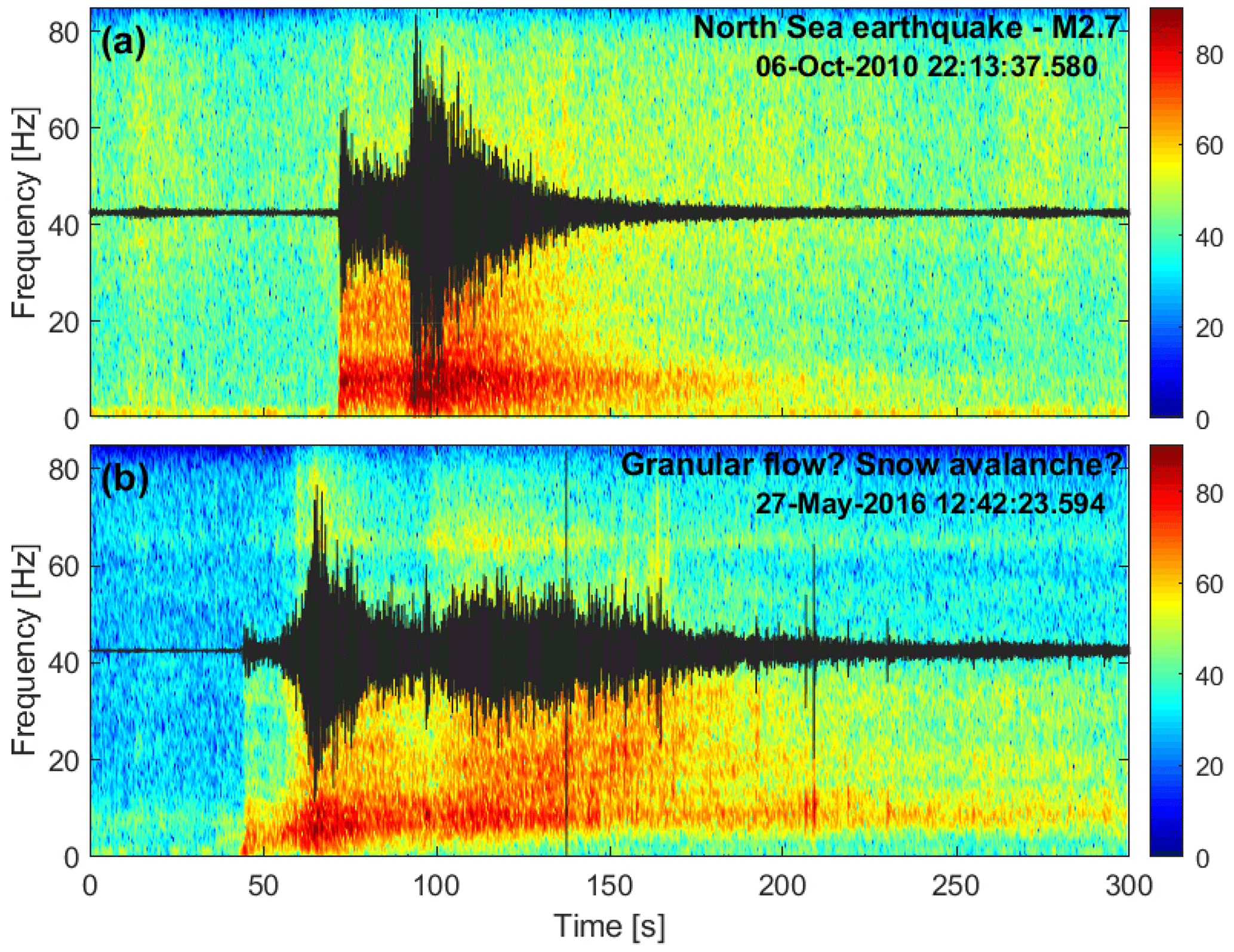
Figure 11 Vertical component records and spectrograms recorded on the broadband seismometer (AKN) showing (a) a M_2.7 earthquake located in the North Sea and (b) an avalanche in late spring 2016, which destroyed the cable to geophone 2. Data are band-pass-filtered in the range 2–80 Hz.

In Fig. 11, we show an example of a regional earthquake and an event on the eastern part of the slope recorded on the broadband seismometer (AKN). In the absence of witnesses, it is difficult to distinguish if the event represents a snow avalanche or a granular flow. The corresponding records of the eight geophones are shown in Figs. B9 and B10 in the Appendix. Although in Fig. 11, the signal characteristics are unequivocal, e.g. with P- and S-wave arrivals clearly identifiable for the earthquake, the 16 s long signals are too short to distinguish between both origins. For the earthquake (Fig. B9), only the P-wave onset was recorded, while the beginning of the trace in Fig. B10 can be misinterpreted as weak P- and stronger S-wave arrival at around 2 and 7 s, respectively. To avoid such misinterpretation, the broadband records could be integrated more systematically into the analysis, whilst in the long term, upgrading the system to obtain continuous records would be the best solution.

Similarly, the observed increase in the number of rockfalls during spring (Figs. 7, B13) may result from a misinterpretation of smaller snow avalanches in the vicinity of the network. Accessing monitoring cameras would help increase the knowledge of the seismic signature of these different surface phenomena.

Another drawback of working with triggered data is that several detections may be contained in a single file. The CNN AlexNet configuration does not allow us to use differently sized spectrogram images. In order to circumvent the limitation, we mask the signal parts in the spectrogram images that are not related to the detection (Fig. B17b). However, many of these events are not well classified; most of them are declared as regional events. This behaviour may also explain the unequal distribution of the number of regional events throughout the year. However, files with multiple detections are relatively seldom, such that the interpretation of the classified events should not be overly affected.

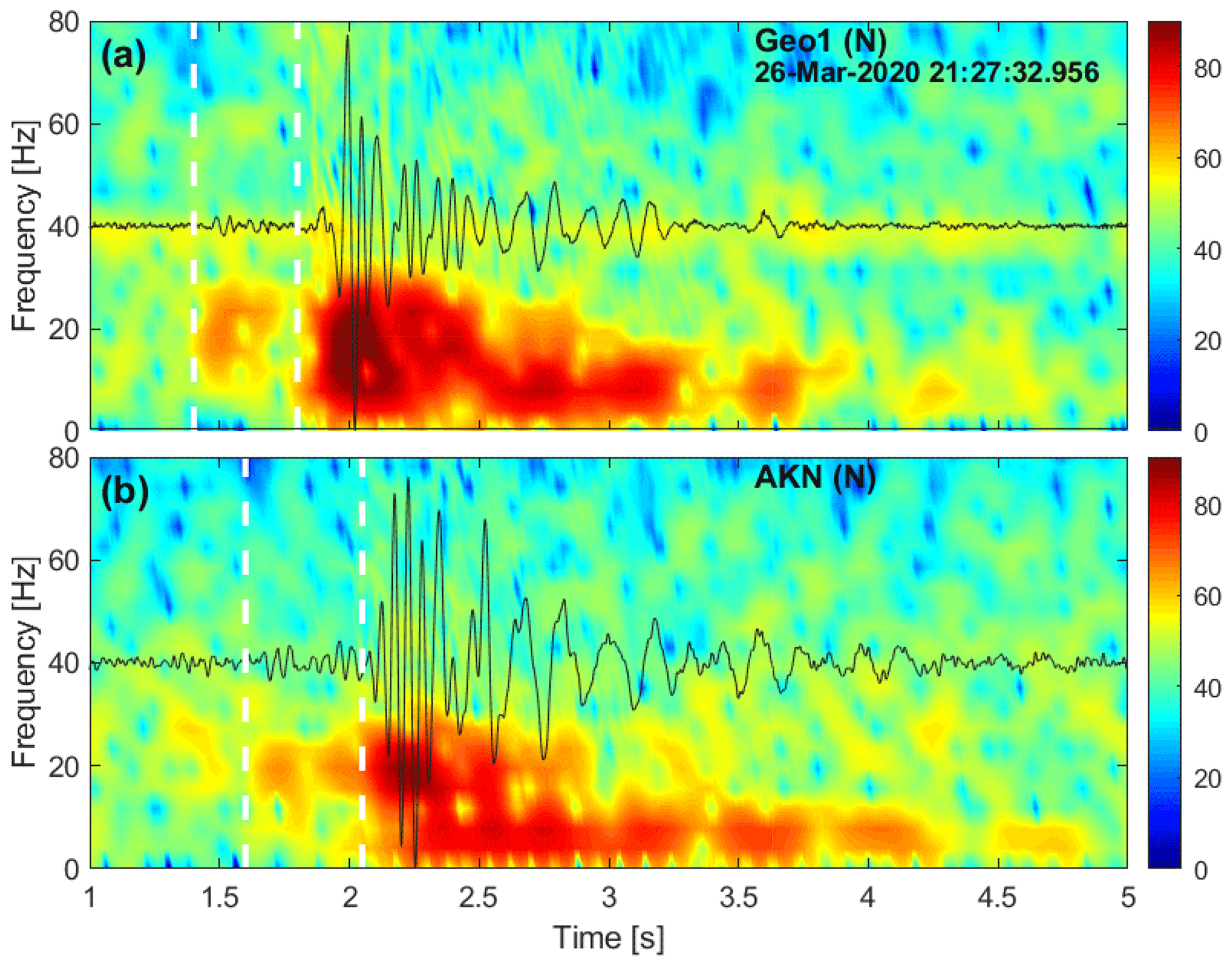
Figure 12 Example of a complex slope quake with precursory signal as defined by Provost et al. (2018). The level of detail necessary for its classification requires higher-resolution computation parameters and is difficult to capture by the CNN. Signal recorded on the north component of (a) a surface geophone; (b) the broadband seismometer (AKN). The white vertical dashed lines mark two phases, the second being the most energetic.

The dataset is not limited to the classes defined in this study and actually contains an even richer diversity of signals (Christiansen, 2021). In particular, complex slope quakes with precursors and hybrid slope quakes as defined by Provost et al. (2018) were found as well. An example of such signals is given in Fig. 12. This example illustrates the complexity of the signals recorded at Åknes and the problem of adapting the classification approach to the case under consideration. The automatic classifier defined the event as an LF slope quake. However, if the computation parameters for the spectrograms are changed to enhance the resolution (here, a sliding window of 0.25 s with a 90 % overlap), a weak, but clear phase emerges before the main burst of energy. On the broadband seismometer (Fig. 12b), a frequency decay of the main peak is visible from approximately 20–30 to 10 Hz after 2.5 s, as would be expected for a hybrid slope quake. This behaviour is less obvious on the geophone (Fig. 12a). In order to explore more classes, the spectrogram computation, for example, would have to be reduced to the event duration, resulting in different sizes of the input images, which is not possible if using a CNN but could be circumvented either by reshaping the images to a fixed size or by using a fully convolutional network. Moreover, events that are recorded simultaneously on the geophone network and the broadband seismometer installed on the central slope are rare; creating a training set with sufficient examples in each class may then become challenging.

Locating the microseismic events could help to better constrain the classification and vice versa. Nevertheless, accurate event location (i.e. enabling us to delineate geological structures at depth such as cracks, fractures, and sliding planes) remains difficult due to the extremely heterogeneous and fractured subsurface material at Åknes. Active seismic profiles were acquired during various field campaigns in summer (Tassis and Rønning, 2019) and show strong velocity contrasts, especially in the back scarp area, ranging from less than 2 km s⁻¹ to more than 5 km s⁻¹ in only 50 m of material. Several attempts were made to locate the events. Fischer et al. (2020) employed a migration-stacking approach and a homogeneous velocity model with a P-wave velocity V_P of 1500 m s⁻¹, fixing the event depth to the surface. In particular, the use of a homogeneous velocity model may be inappropriate. More recent attempts using a 3D velocity model resulting from the combination of both check shots and seismic refraction profiles did not yield event locations within reasonable uncertainty limits, i.e. not more than a few tens of metres (Dahl, 2020). Since, depending on the study, the sliding plane depth has been estimated as being between 50 and 120 m (e.g. Kveldsvik, 2008; Nordvik et al., 2009), a sufficient depth resolution of event locations is required. In addition, locating the events is hampered by the proper identification of the phases in the seismograms as illustrated in Fig. 12. Inverting the proper observations with the correct associated velocity model is fundamental whatever type of location algorithm would be used (e.g. the picking or migration-stacking approach).

Finally, although the classifier delivers satisfying results (Fig. 5), it still can be improved. First of all, the spectrogram stacking approach is not optimal, especially for signals exhibiting a strong variability in their waveforms for different geophones (e.g. Figs. B4 and B5) such as rockfalls. One way of tackling the problem would be to classify each spectrogram separately. The chosen class could be the predominant one or the one which returns the largest combined probability. In addition, such an approach would enable us to significantly increase the size of the training set, which could ultimately result in even better-defined classes, taking into account all the existing waveform variability (Lee et al., 2022). Secondly, events related to surface processes such as rockfalls and snow avalanches lack ground truth. This could be partially resolved if web cameras were available. Even though it is not possible to monitor the whole slope, only a few exemplary observations of events of each class would be sufficient to identify the related signal characteristics.

6 Conclusions and perspectives

In this paper, we characterized and automatically classified seismic signals recorded by an eight-geophone surface network on the Åknes unstable rock slope. Five classes of events directly related to the slope could be identified following the typology proposed by Provost et al. (2018), including HF, LF, and successive slope quakes, short tremors, and rockfalls. Fifteen years of data, corresponding to approximately 60 000 events, was classified and analysed.

Similarly to the observations by Fischer et al. (2020), the seismic activity displays a strong seasonality with the majority of events occurring in spring, corresponding to both the period of snowmelt and temperatures oscillating around the freezing point. This observation is in agreement with displacement rates of the Åknes slope which feature seasonal variations as well, i.e. acceleration in spring and autumn (Grøneng et al., 2011).

This periodically increased seismic activity is accompanied by a significant increase in the number of detected low-frequency slope quakes, tremors, and rockfalls. Comparatively, the number of high-frequency and successive slope quakes seems to remain almost stable throughout the year. Our hypothesis is that HF and successive slope quakes are related to shearing on the sliding plane. LF slope quakes and tremors, on the other hand, are associated with the thawing–freezing process within small cracks. Since tremors are more frequent during the daytime, they could be related to water movement within newly created cracks after thawing, while LF slope quakes could correspond to the back scarp opening and the formation of new cracks. It is difficult to distinguish if the apparent increase in rockfall activity in spring is realistic or if it is caused by other surface processes such as local snow flows. Their increase at the beginning of autumn coincides with increased precipitation. Finally, larger events such as snow avalanches and granular flows may occur but are more difficult to characterize without continuous data and ground truth.

No correlation of the seismic activity with precipitation could be established in this work. For example, strong rain episodes (> 100 mm within a day) are not necessarily followed by an increase in the microseismic activity. This does not mean that such a correlation does not exist, since for example increases in the groundwater level are correlated with higher displacement rates (Nordvik and Nyrnes, 2009). However, recent work aiming to better understand the hydrogeological system at Åknes emphasized its complexity and showed the existence of barriers maintaining a high groundwater level at high elevation (e.g. Sena and Braathen, 2021; Pless et al., 2021). Establishing potential systematic correlations between classified microseismicity, precipitation, and groundwater level fluctuations should be the subject of future work.

In the future, we plan to take advantage of the seismic data recorded by the broadband seismometer and the borehole geophones that have been installed on the slope but are not yet part of the monitoring system. Since these instruments record data in a continuous mode, they may help provide more exhaustive catalogues of microseismicity. Last, but not least, the classifier implemented in this study, which is based on stacked spectrogram images and avoids the explicit definition of features, achieves a success rate of up to 80 %. Its performance could be improved further by applying ensemble prediction on individual spectrograms and by applying more advanced techniques such as self-supervised learning (Lee et al., 2022). Recently, random forests for classification purposes were also successfully applied to continuous streams of seismic data (e.g. Chmiel et al., 2021; Wenner et al., 2021). Although not tested in this work due to the limitation of the dataset to triggered data only, the CNN workflow should be adaptable to continuous data by defining moving time windows, similarly to the work of Takahashi et al. (2021), where tremors, earthquakes, and noise recorded on a single station were automatically classified. Automatic detection of signals could possibly be added to such an implementation through class activation maps (Zhou et al., 2016).

Appendix A: Detection

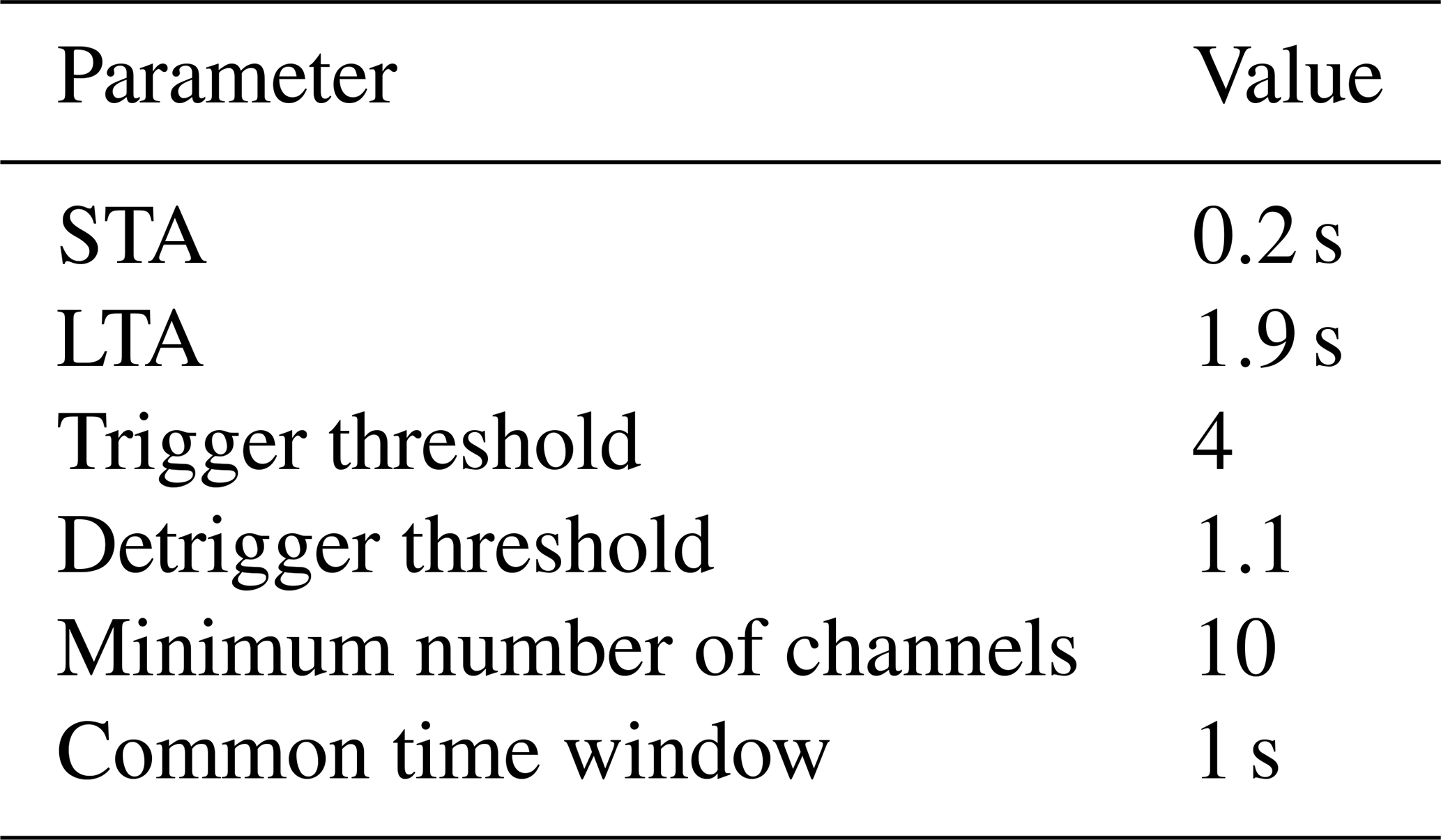
Microseismic events are detected via STA/LTA (Withers et al., 1998). Computation and detection parameters are provided in Table A1. An event is detected if the trigger criteria are met at a minimum number of channels within a given time window.

Table A1 STA/LTA parameters used for event detection.

Appendix B: Classification

B1 Diversity of seismic signals

Figures B1 to B8 show the vertical component records (left) and associated spectrograms (right) of the example signals plotted in Fig. 2 to illustrate either the relative similarity or the variability of the waveforms across the geophone network.

Figure B1 Example of a high-frequency (HF) slope quake. Geophone 7 was not functional.

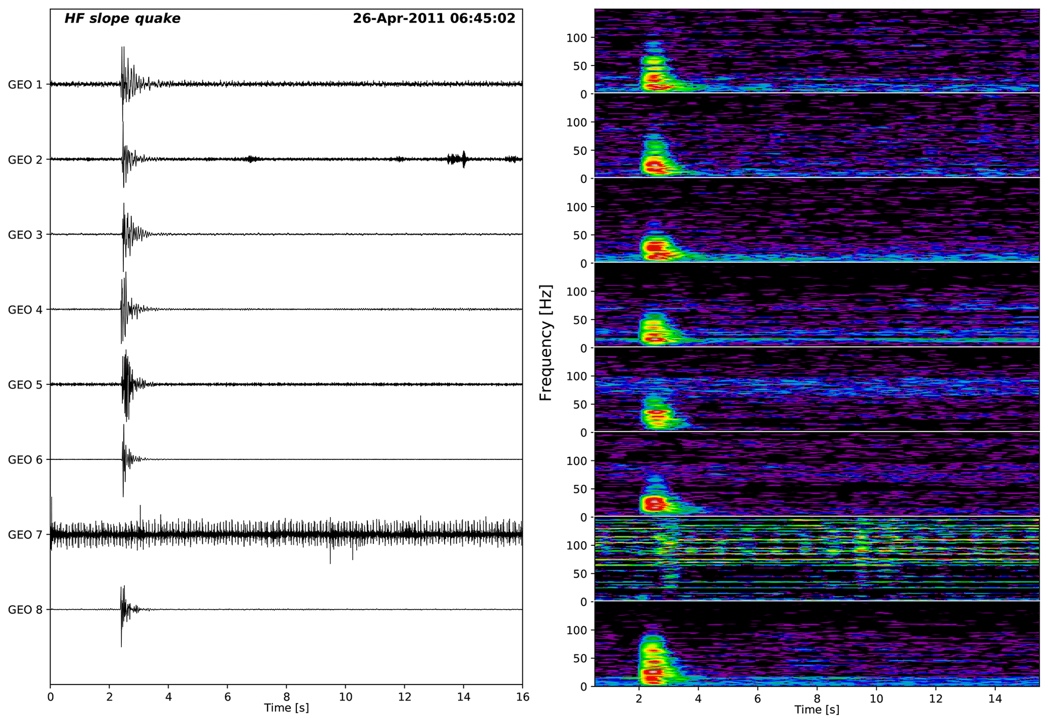
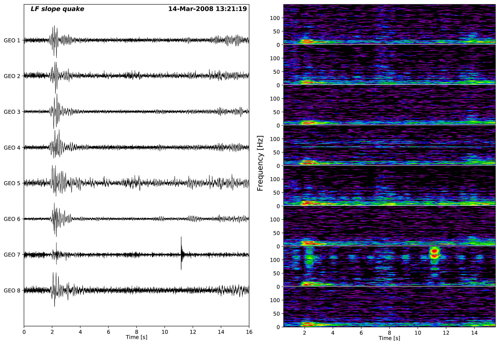
Figure B2 Example of a low-frequency slope quake. A stronger spurious signal was recorded on geophone 7.

Figure B3 Example of a tremor-like slope quake.

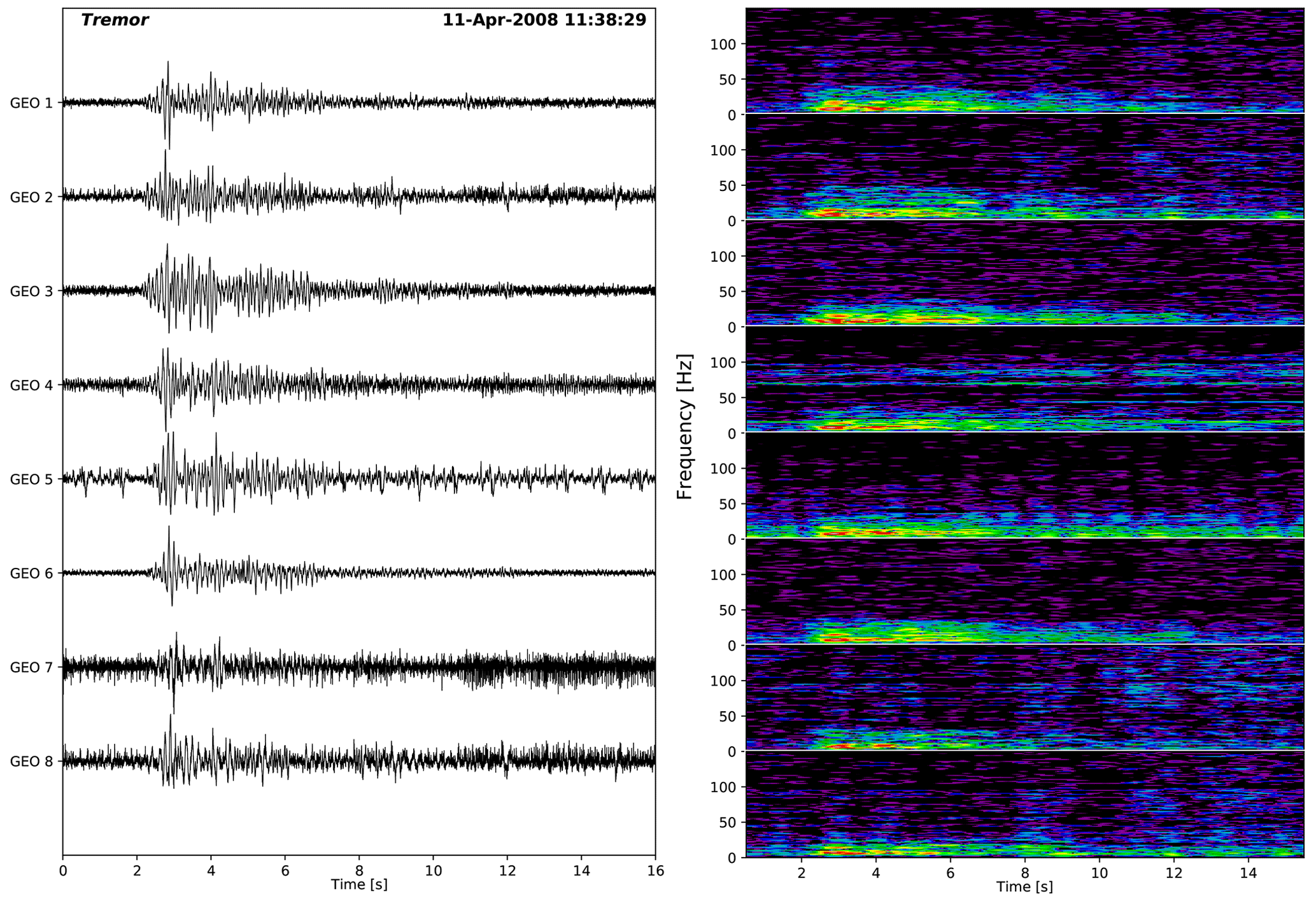
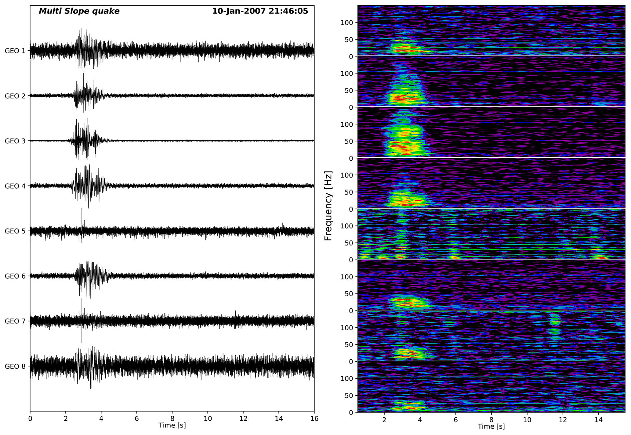
Figure B4 Example of a succession of slope quakes. Geophone 5 was not functional, while geophones 1, 7, and 8 were noisy.

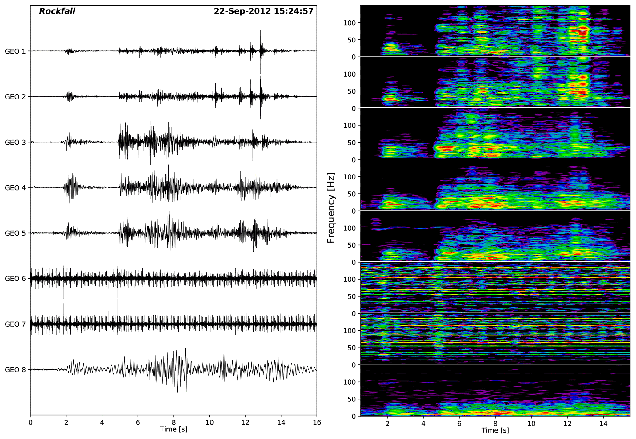
Figure B5 Example of a rockfall. Note the distinctive variability of the waveforms across the geophones. Geophones 6 and 7 were not functional.

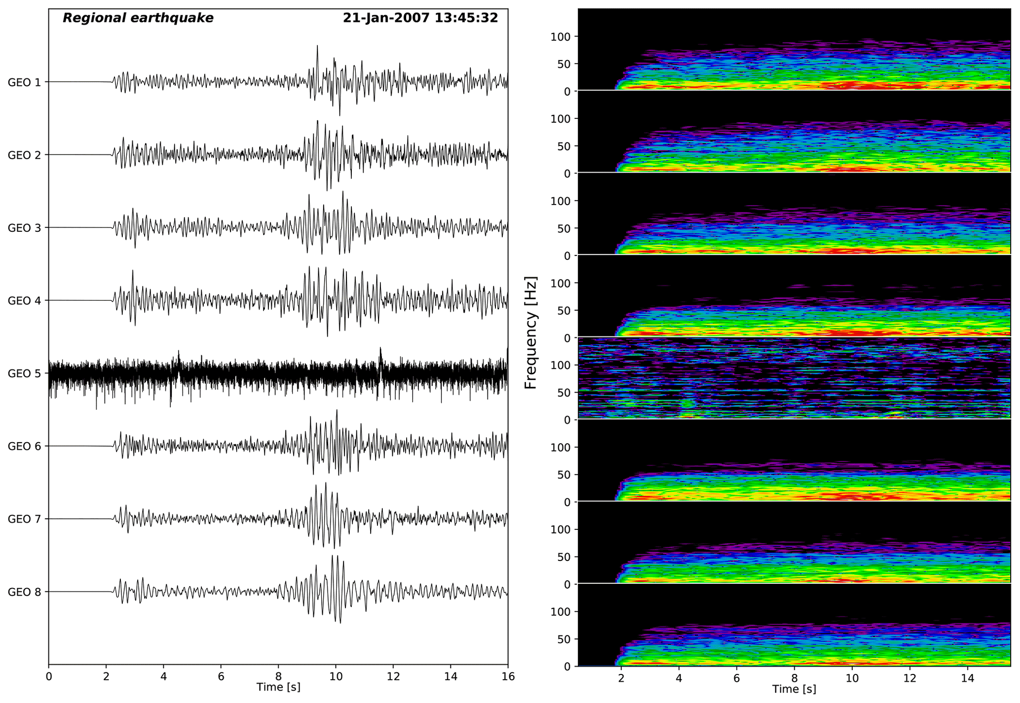
Figure B6 Example of a regional earthquake. P- and S-wave arrivals are clearly identifiable. Geophone 5 was not functional.

Figure B7 Example of an electric spike.

Figure B8 Example of a noise record.

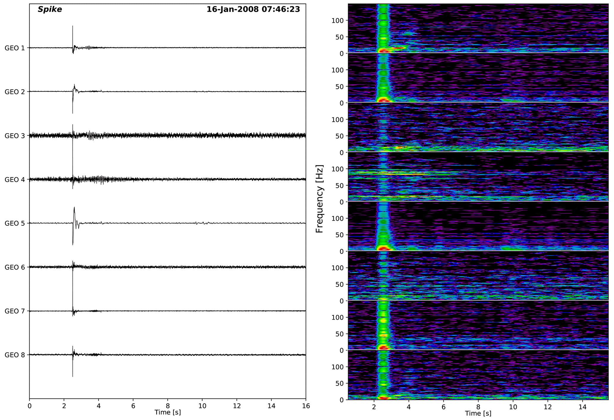
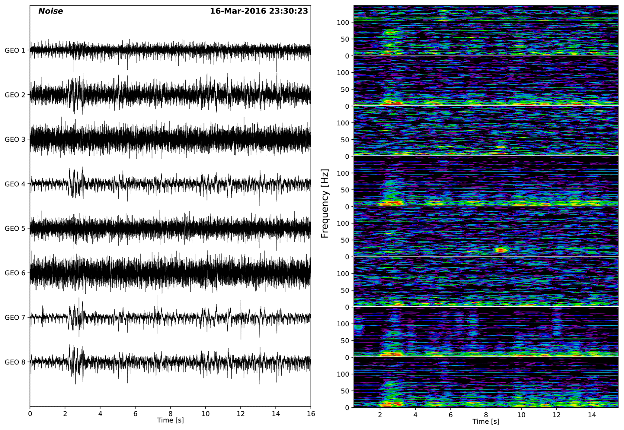
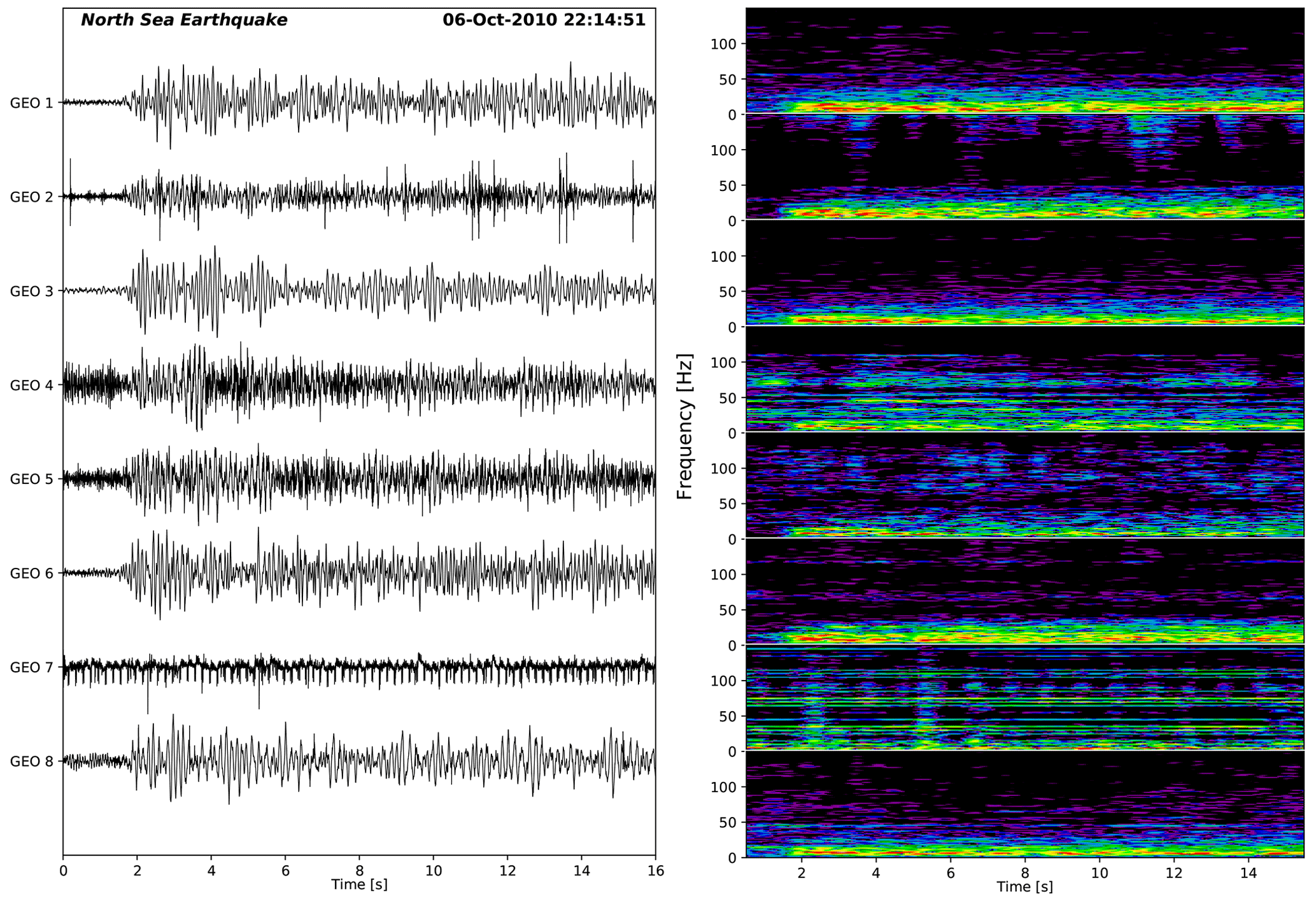
Figure B9 Example of a regional earthquake of magnitude M_2.7 located in the North Sea, SW of Åknes. Due to the distance of the hypocentre to the stations, only the P-wave arrival is visible on the 16 s long records. Waveforms recorded on geophones 2 and 4 are noisy and show greater variability compared to the other waveforms. Geophone 7 was not functional.

Figure B10 Vertical component traces of the event shown in Fig. 11. A first, weak arrival is visible around 2 s before a second, stronger arrival at 8 s. These observations are misleading and could be wrongly interpreted as P- and S-wave arrivals, respectively.

B2 Classifier

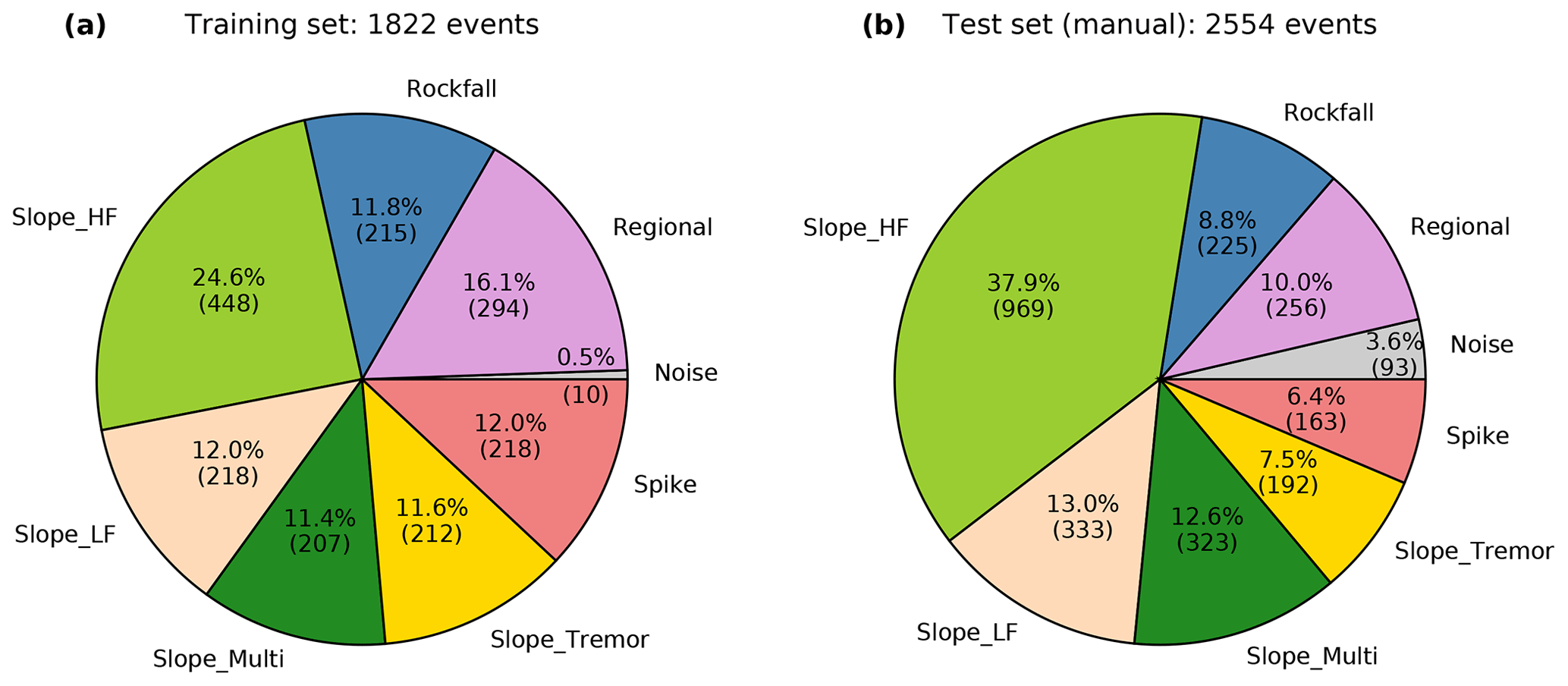
Figure B11 Pie diagrams showing the distribution of events within the different classes (a) in the training set and (b) in the test set, both expressed in terms of number of events and percentages.

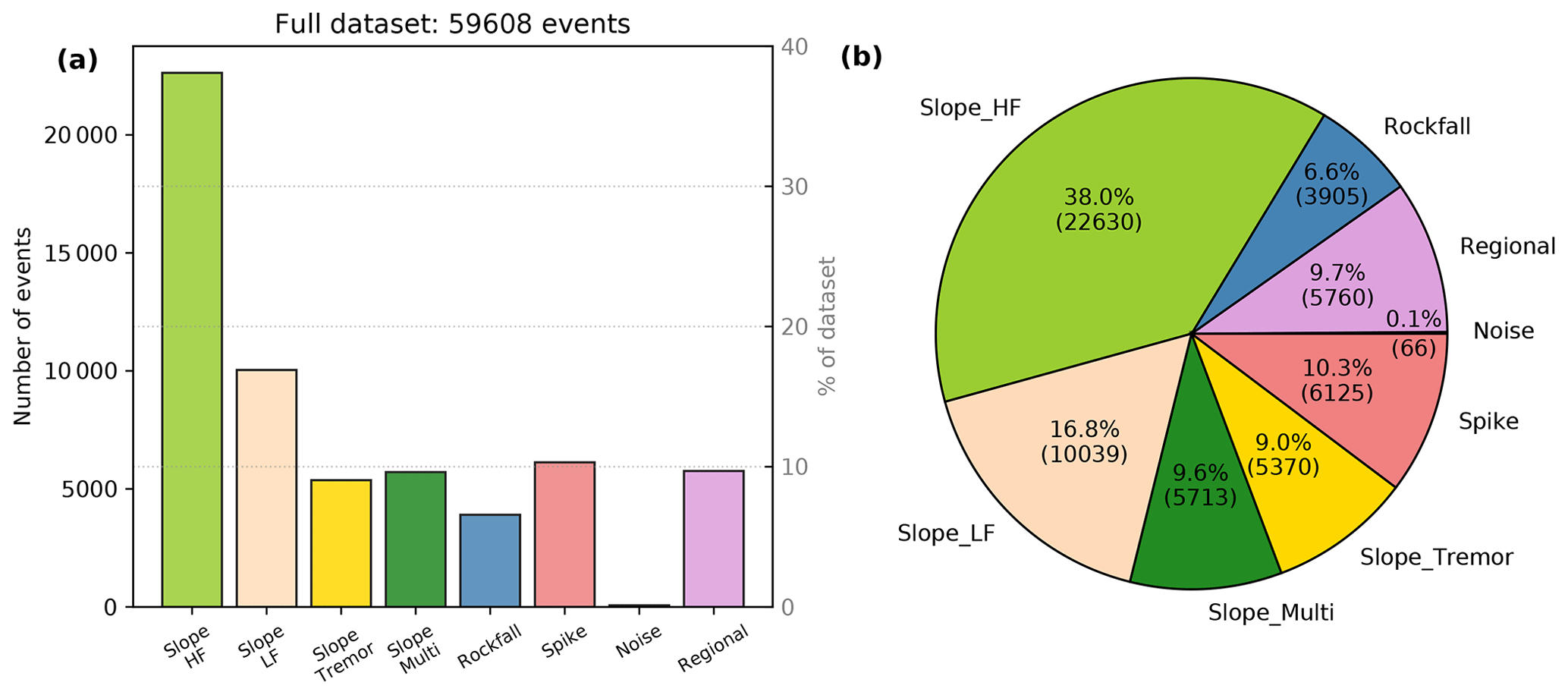
Figure B12 Distribution of automatic classes over a time period of 15 years (2007–2021): (a) histogram; (b) pie diagram.

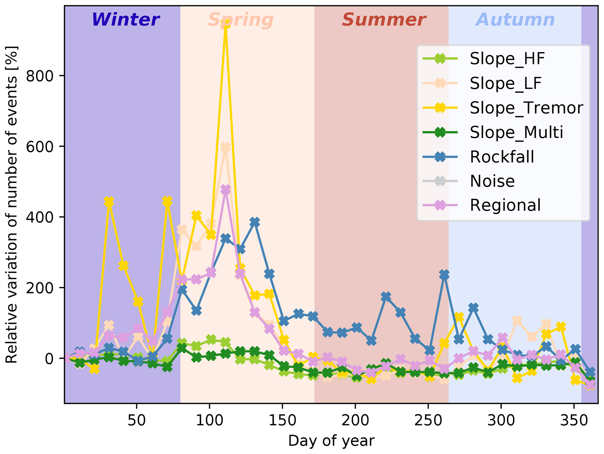
Figure B13 Relative variations R of the number of events N per class over chunks of 10 d. The reference value is taken from the first chunk; i.e. we compute $R=(N-N(\mathrm{1}\left)\right)/N\left(\mathrm{1}\right)$. Note that noise events are so rare that they are not visible in the plot.

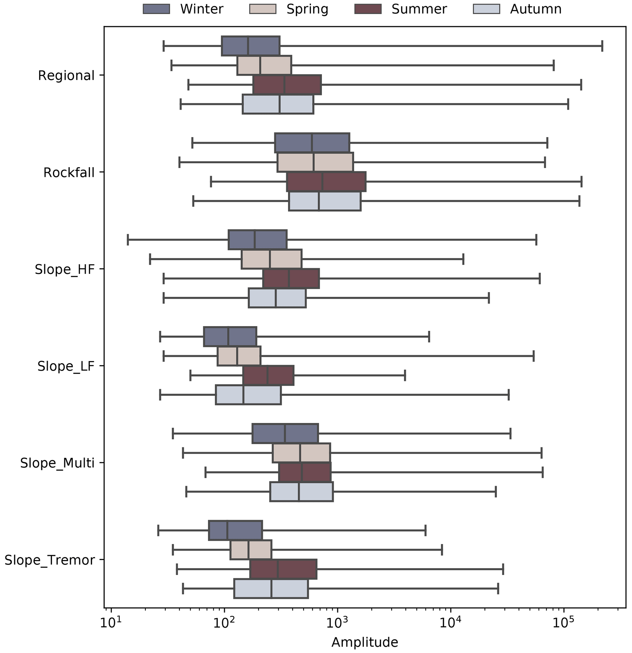
Figure B14 Box plots showing the distribution of amplitudes for each event class by season. Amplitudes in summertime are systematically higher than during the rest of the year.

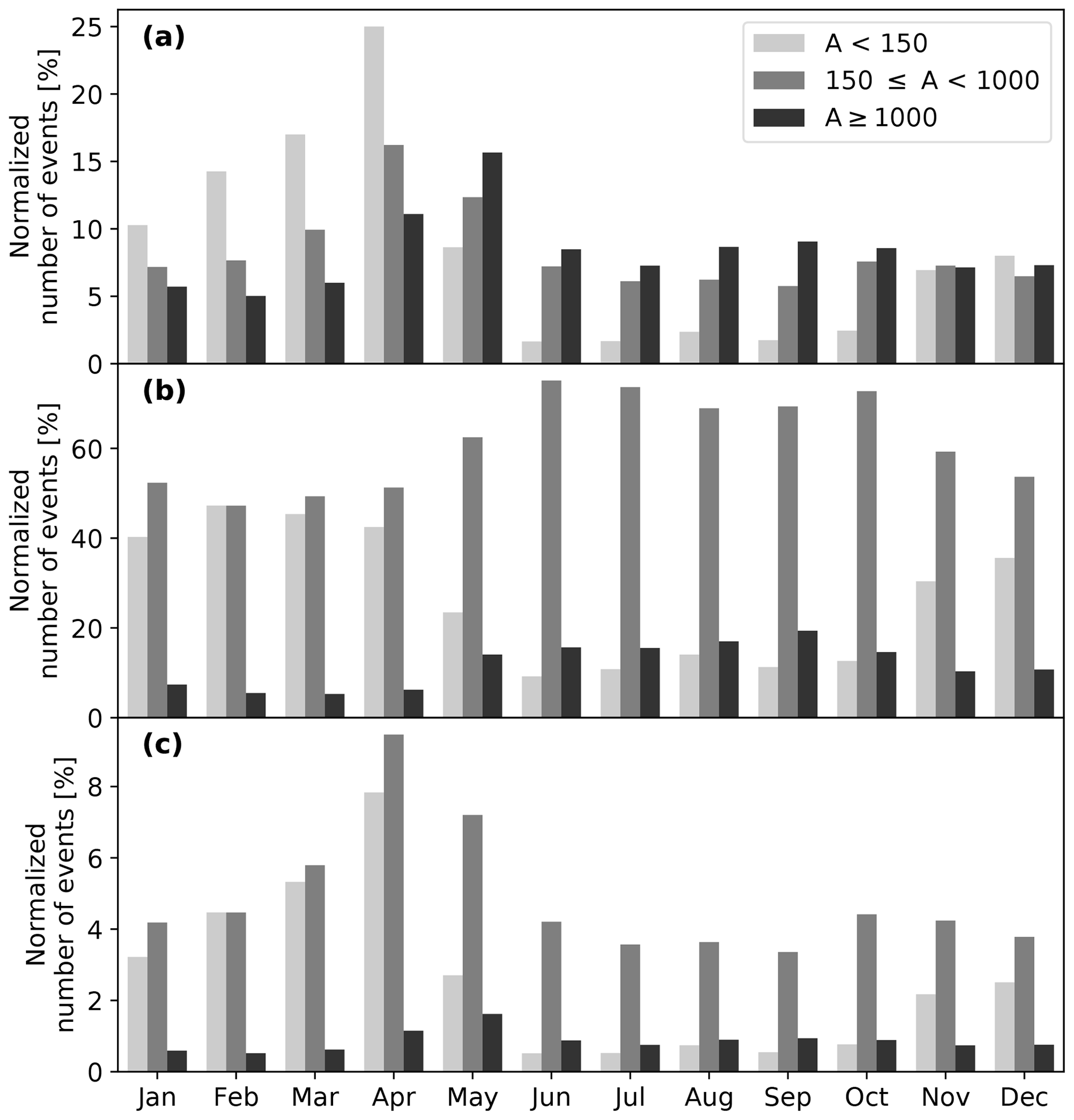
Figure B15 Histogram showing the distribution of events of lower amplitude (light grey), intermediate amplitude (grey), and higher amplitude (dark grey) over months. The number of events is normalized in (a) by the total number of events in the different amplitude ranges, in (b) by the total number of events per month, and in (c) by the total number of events in the dataset. The deficit in low-amplitude events from June to October is particularly visible in all cases. A seasonal variation in the proportion of intermediate and high-amplitude events exists as well but to a much lesser extent.

Figure B16 Box plots showing the distribution of amplitudes for each event class.

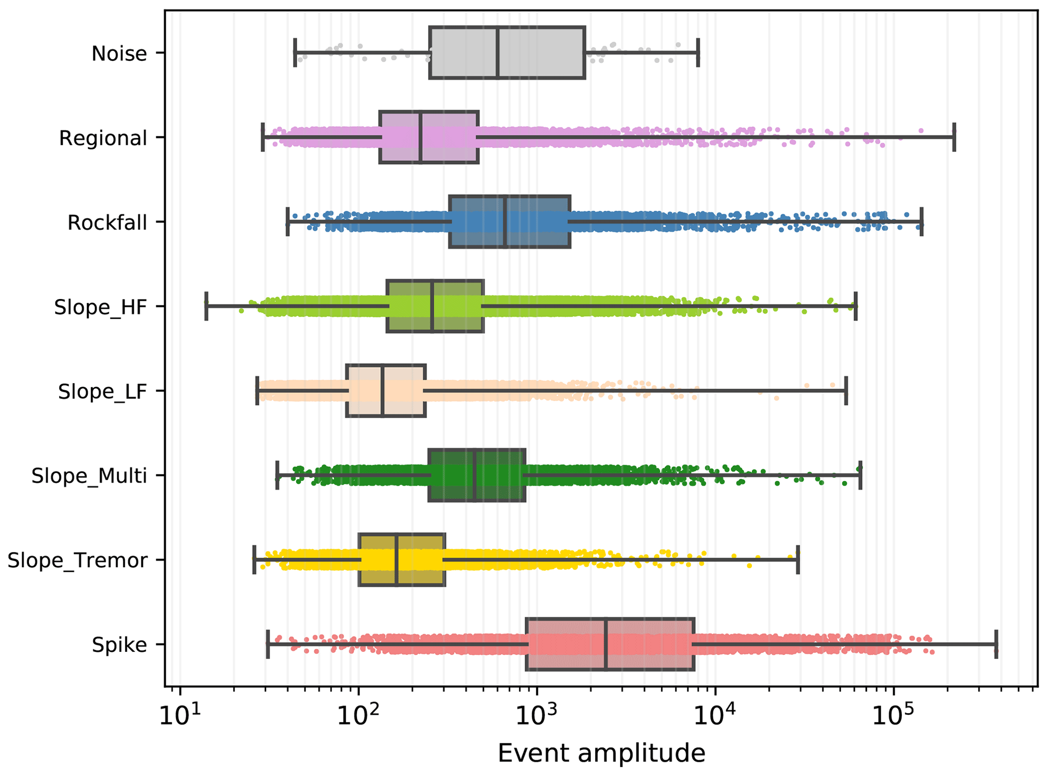
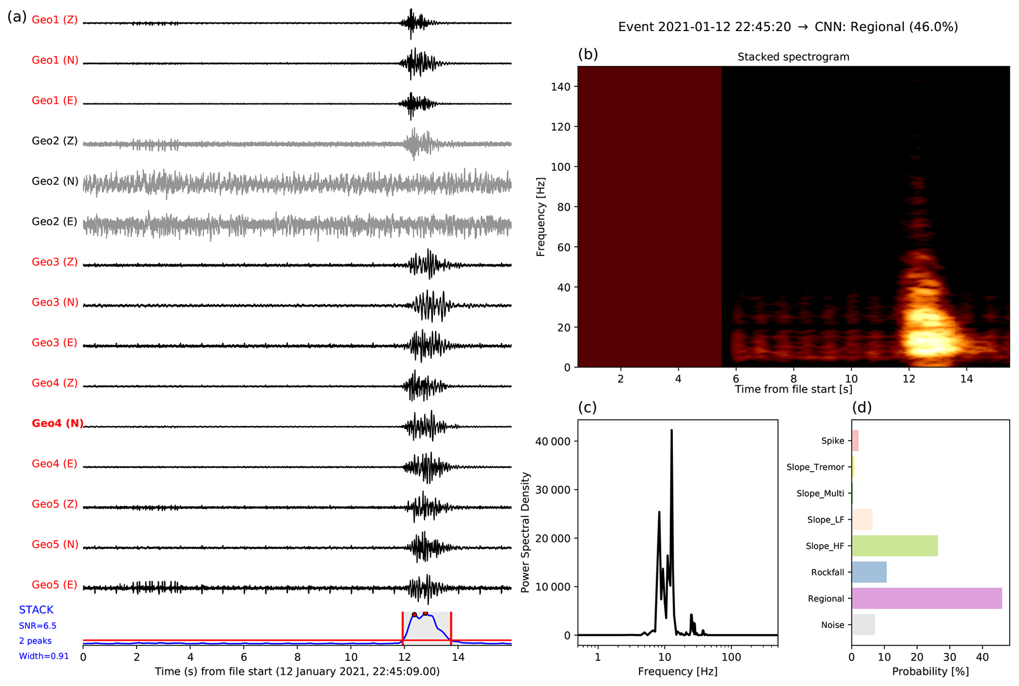
Figure B17 Example of an event wrongly classified as a regional earthquake instead of an HF slope quake; see Fig. 4 for description. Note that we only display the waveforms at geophones 1 to 5, since geophones 6–8 were not functional. The event file contains two events and detected electric noise at around 2 s. A mask was applied on the spectrogram image but cannot prevent misinterpretation. However, (d) illustrates that the probability of being a regional event is relatively low (below 50 %) and the probability of being an HF slope quake is not much lower.

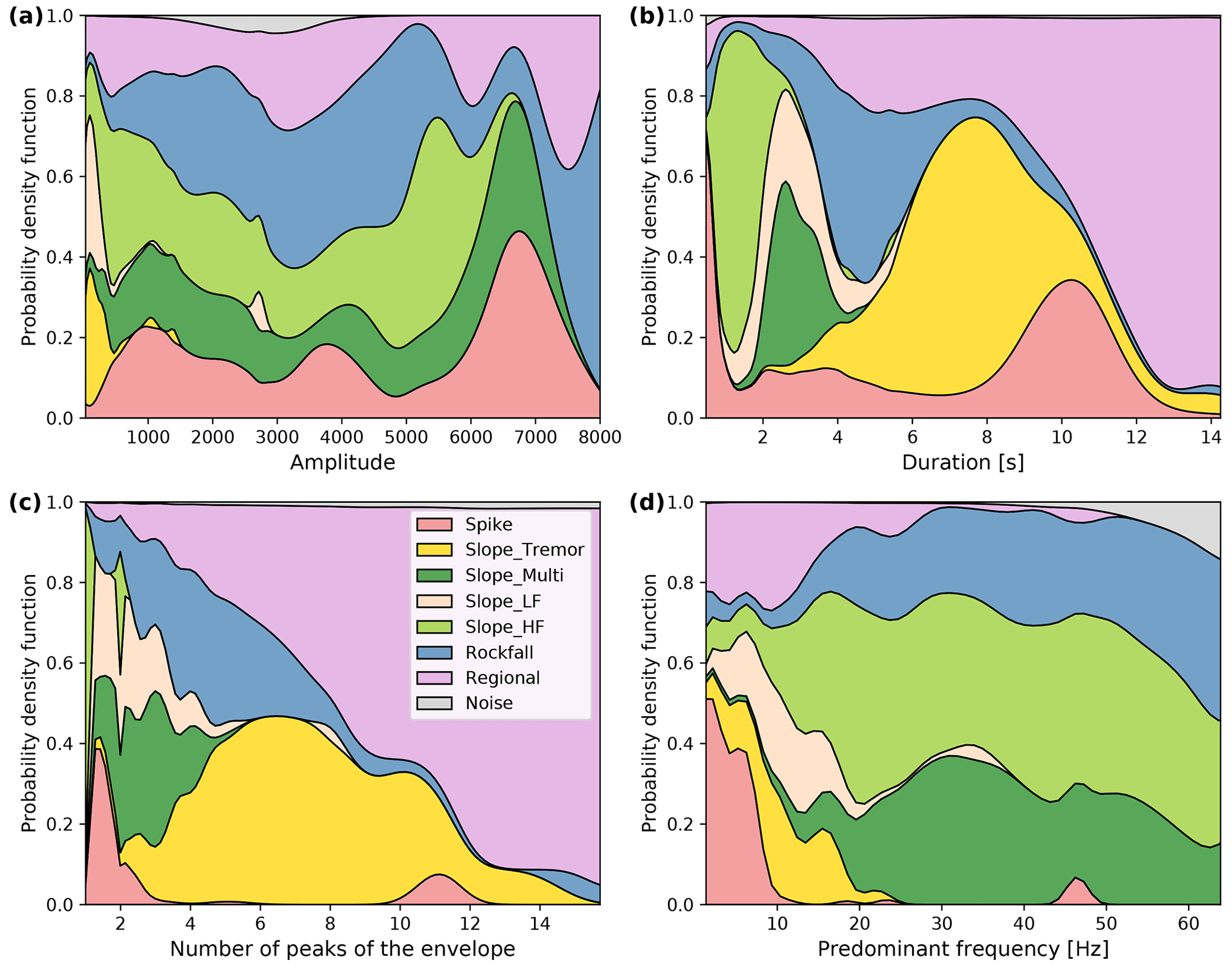
Figure B18 Probability density functions of some extracted features from the training set. Although the CNN is not a feature-based algorithm, it is interesting to look at the distribution of those features since they are the ones that a human eye would subconsciously catch and analyse while manually labelling the data.

Appendix C: Meteorological data

The meteorological station is located in the vicinity of the upper bunker (Ørnereiret) close to the top scarp. Temperature and precipitation are measured and averaged hourly.

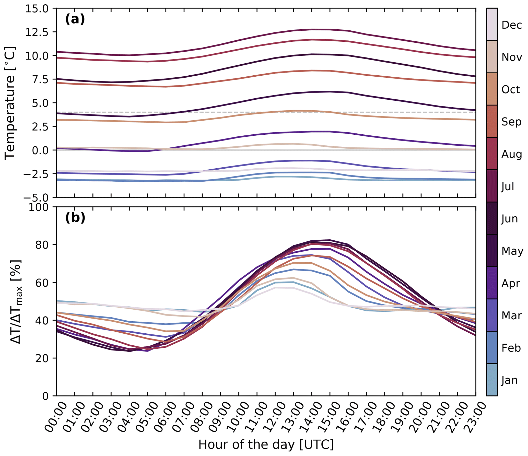
Figure C1 Temperature variations recorded at Åknes. The measurement period spans 15 years (January 2007–December 2021). (a) Hourly variations in average temperature for each month of the year. To obtain the relative variations shown in (b), the curves in (a) were normalized by their minimum and maximum values: $\mathrm{\Delta }T/\mathrm{\Delta }{T}_{max}=(T-T_{\min })/(T_{\max }-T_{\min }$).

Figure C2 Distribution of the number of days per year when the average temperature is lower than 0 ^∘C (dark blue), between 0 and 4 ^∘C (light blue), or above 4 ^∘C (light red). Hatches correspond to days in the first half of the year (1 January to 30 June). The number of days when the average temperature is between 0 and 4 ^∘C during spring is indicated. Days with outliers (abnormally small or high temperature values) are removed.