the Creative Commons Attribution 4.0 License.
the Creative Commons Attribution 4.0 License.
 | 03 Jan 2024
Stochastic properties of coastal flooding events – Part 1: convolutional-neural-network-based semantic segmentation for water detection
Byungho Kang
Rusty A. Feagin
Thomas Huff
Orencio Durán Vinent
The frequency and intensity of coastal flooding is expected to accelerate in low-elevation coastal areas due to sea level rise. Coastal flooding due to wave overtopping affects coastal communities and infrastructure; however, it can be difficult to monitor in remote and vulnerable areas. Here we use a camera-based system to measure beach and back-beach flooding as part of the after-storm recovery of an eroded beach on the Texas coast. We analyze high-temporal resolution images of the beach using convolutional neural network (CNN)-based semantic segmentation to study the stochastic properties of flooding events. In the first part of this work, we focus on the application of semantic segmentation to identify water and overtopping events. We train and validate a CNN with over 500 manually classified images and introduce a post-processing method to reduce false positives. We find that the accuracy of CNN predictions of water pixels is around 90 % and strongly depends on the number and diversity of images used for training.
- Article
(8259 KB) - Full-text XML
- Companion paper
- BibTeX
- EndNote


Coastal flooding can cause significant damage to coastal infrastructure, communities, and salt-intolerant ecosystems. By definition, flooding occurs when extreme water levels – due to a combination of high tide, wave runup, and/or storm surge – exceed a natural or artificial threshold, e.g., a beach berm, dune, or seawall. The frequency and severity of coastal flooding is expected to increase with the acceleration of sea level rise (Nicholls et al., 2011; Vitousek et al., 2017). In order to respond to and minimize the damage from coastal flooding, it is crucial to determine the frequency and intensity of flooding events at different locations and identify the physical factors behind them (Hallegatte et al., 2013; Moore and Obradovich, 2020). This is particularly relevant for high-frequency and low-intensity nuisance flooding not directly associated with large storms that is thus difficult to predict and detect (Moftakhari et al., 2018).
Over spatial scales on the order of kilometers or larger and on timescales on the order of minutes or larger, water levels are usually estimated from tidal gauges, while existing predicting tools can also account for wind-induced water levels (Huff et al., 2020). Although these results can be interpolated fairly well to cover locations between gauges, they still fail to capture the contribution of local wave runup. Wave runup, most typically measured by R2 %, can greatly exceed the average predicted water level by other methods or sensors, resulting in the overtopping of coastal dunes and seawalls. This is because runup is a function of wave height and wavelength (Battjes, 1974) and thus depends on wave interaction with the bathymetry and topography (Strauss et al., 2012; Vitousek et al., 2017). In spite of several empirical formulas to estimate wave runup from offshore wave data (e.g., Stockdon et al., 2006, 2014), accurately predicting wave runup is difficult because wave interaction is spatially localized. Furthermore, wave height and length are individualized measures that longer-temporal-scale gauges are not designed to detect.
Fortunately, the excursion extent of the water level at these localized spatial and temporal scales can be generally represented by the existence of the wet–dry line along a sandy beach. Specially designed camera systems are now commonly used to monitor local wave runup, aiding in the refinement of empirical formulas and the increased understanding of runup's stochastic properties. Over nearly 4 decades, the evolution of optical remote sensing technologies has revolutionized wave runup monitoring, moving from manual digitization (Holman and Guza, 1984) to modern camera-based systems that efficiently capture wave runup and shoreline (Holman and Stanley, 2007).
Indeed, a lot of data are available online that could potentially be mined to help improve coastal flooding predictions if we had automated methods to classify the wet–dry line in these images. For example, Vousdoukas et al. (2011) applied a classical machine learning model with a three-layer artificial neural network (ANN) to determine the pixel intensity threshold and estimate the elevations of shoreline contours. Likewise, Alvarez-Ellacuria et al. (2011) applied ANN to a time exposure image to determine the shoreline. Using a structured support vector machine (SVM), Hoonhout et al. (2015) estimated beach width and the location of the water line based on semantic classification of mid-range coastal imagery and proved the robustness of such a technique for the long-term analysis of the coastal imagery. More recently, the US Geological Survey has also begun to harness the power of SVM to augment the edge detection algorithm to identify the runup edge (Palmsten et al., 2020).
An important limitation of the aforementioned computer vision techniques is that they require calibration or feature extraction pre-processing at the initial stage. Therefore, in-depth knowledge was essential for each method, which has prevented their widespread use. This limitation can be overcome using “deep learning” algorithms such as convolutional neural networks (CNNs).
The “deep learning” movement started in the mid-2000s when Hinton et al. (2006) rekindled the use of the neural network in machine learning by showing the networks with many hidden layers could also be trained as well. Following this work, the introduction of the rectified linear unit (RELU) for multi-layer back-propagation has led to the widespread use of CNNs for image recognition, which inherently has deep architecture (Nair and Hinton, 2010; LeCun et al., 1989). Breakthroughs of deep convolutional neural networks in image classification have been transferred to pixel-level semantic segmentation (Chen et al., 2016), since a fully convolutional network based on decoder structure outperforms other classical machine learning models in terms of pixel accuracy (Long et al., 2015).
Image segmentation based on CNN has been applied to various video-based coastal studies. Buscombe and Ritchie (2018) introduced a hybrid model that combines fully connected conditional random field (CRF) and CNN platform to analyze large-scale coastal imagery. Valentini and Balouin (2020) used the same method with the base of Simple Linear Iterative Clustering (SLIC) super-pixels instead of fixed tiles to detect and monitor Sargassum algae for an early warning system. The approach was convenient and accurate, as it relied on a predefined dataset for the classification, which does not require exhaustive manual annotations. However, this segmentation process was based on the classification of tiles – a bundle of pixels – rather than actual “pixels”. Thus, the minimal resolution was often too low to classify features smaller than the size of tiles and super-pixels. Furthermore, Sáez et al. (2021) used an U-net architecture for detecting wave-breaking nearshore while other studies had tried to validate semantic segmentation by comparing with other measurement methods. For example, by comparing the results with gauges in a physical model test, den Bieman et al. (2020) showed that image segmentation by SegNet can reasonably predict surface elevation, runup, and bed level from video images.
In terms of flooding management, studies conducted by Muhadi et al. (2021) and Vandaele et al. (2021) have shown the reliability of image segmentation for fluvial water level estimation. In those studies, the correlation between estimated water level and the water level estimation from lidar data and river gauge measurement was higher than 0.9, which signals potential use for coastal flooding analysis.
In this work, we explore the use of CNN-based semantic segmentation to automatically detect water on beach imagery and to identify and quantify coastal flooding events. In addition to a brief introduction to CNN-based image segmentation, we discuss the specific methodology used for this study and present a simple but powerful post-processing method for refining the accuracy of semantic segmentation. We then investigate the performance of the method as function of morphological diversity and the number of images in the training set.
In order to test CNN methods, we collected field data at a heavily eroded location after Hurricane Harvey struck the Texas Coast in 2017 and explored the imagery using CNN. We provide a basic overview of CNN and the Deeplab architecture used in our analysis and discuss the collection and annotation of the images used for training and validating the CNN.
2.1 Semantic segmentation using CNN
For the CNN architecture, we selected the Deeplab v3+ model based on Resnet-18, which adds some unique features to semantic segmentation such as the Atrous or Dilated convolution. Independently introduced by Chen et al. (2016) and Yu and Koltun (2015), embedding the holes to the convolution filters has helped to circumvent the resolution loss from downsampling by enlarging the field of view with a lower computational cost. Furthermore, batch normalization layers have been included in each of the parallel modules in the Atrous Spatial Pyramid Pooling (ASPP) module. Normalization over a mini-batch minimizes the transition in the distribution of internal network nodes (covariate shift) and assures the distribution of nonlinear inputs remain more robust (Ioffe and Szegedy, 2015). This helped to fix the vanishing gradient problem, and hence it accelerated the training of the deep neural network. Concatenated results from the parallel modules and image-level features were passed through 1×1 convolution and provide more accurate results (Chen et al., 2017).
Deeplab v3+ also has a unique decoder module to refine the details of object boundaries that extends the previous versions. Instead of naive bilinear up-sampling the encoder features by a factor of 16, the encoder features are first bilinear up-sampled by a factor of 4 and concatenated with the result of 1×1 convolution of low-level features (Chen et al., 2018). The 3×3 convolutions are then applied for the refinement, which is followed by another up-sampling by a factor of 4.
In this study, we conduct regular convolution instead of depth-wise separable convolution typically used for Deeplab v3+ structure, as the Resnet-18 has relatively shallow layers (18 layers) and the computation burden is not heavy, such that we do not have to reduce the number of weights at the cost of accuracy.
2.2 Data acquisition and classification
We installed three solar-powered stationary GoPro cameras, with different fields of view, near Cedar Lakes in Texas (28.819∘ N, 95.519∘ W) to monitor beach recovery after Hurricane Harvey in 2017 (Fig. 1). We hypothesized that this site would experience more flooding events after the beach erosion following the storm. We preset each camera to capture pictures every 5 min during a 06:00–18:00 LT observation period and turn off automatically during the nighttime. From November 2017 to May 2018, we captured more than 51 000 images.
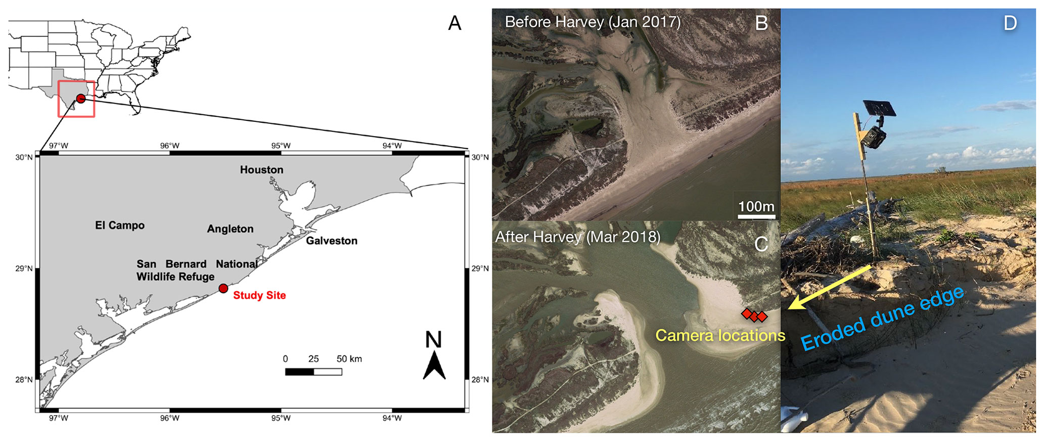
Figure 1Location of field observations (a). Satellite view of Cedar Lakes, Texas, before Hurricane Harvey (b). Three solar-powered cameras (c, d) were installed in Cedar Lakes, a site breached during Harvey that experienced frequent flooding afterwards. (b, c) Map data: © Google, Landsat/Copernicus.
We chose 584 random pictures with different scenery, weather, and light conditions (Fig. 2) and manually labeled the regions on each picture according to three classes: “water”, “sky”, and “background”, where the sky class was added to reduce false positives of water pixels (Fig. 3). We refer to the classes as labels when describing the pixel in an image.
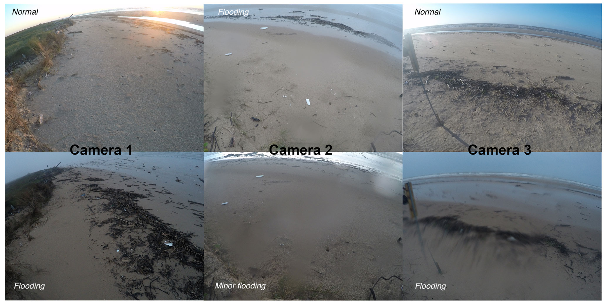
Figure 2Contrasting images captured from our three cameras depicting both flooding and normal conditions.
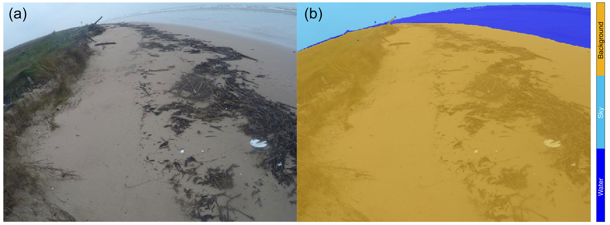
Figure 3A example of a picture taken during flooding conditions (a) with manual labels superimposed (b).
Every pixel was annotated by hand for each class to improve accuracy. We opted not to utilize the SLIC super-pixel method, a commonly employed computer vision technique for labeling, as it often resulted in clusters of pixels containing more than two classes. We then divided the 584 annotated pictures into a training set with 493 images (85 %) and a validation set with 91 images (15 %).
2.3 Training protocol
We used transfer learning (Bengio, 2012), which can expand the use of deep learning for the limited training dataset. We transferred the parameters of Resnet-18 that had been pre-trained using the subset of the ImageNet database for ImageNet Large-Scale Visual Recognition Challenge (ILSVRC) (Russakovsky et al., 2015). After this, we re-train the network with our training images using MATLAB Deep Learning Toolbox as a module.
Both the training images and the manual annotations were compressed from 1920×2560 to 480×640. For every iteration during the training, we flipped each image horizontally with 50 % probability to avoid over-fitting. The mini-batch size was four. To deal with the local minimum problem, images were shuffled randomly for every epoch.
We choose stochastic gradient descent (SGD) with momentum for the optimization algorithm (Wilson et al., 2017) and set the momentum as 0.9. We also replaced the standard classification layer with the classification layer that uses the weighted cross-entropy loss. This was done in order to offset the imbalanced classes induced by the backgrounds that cover more than 80 % of almost every image (Eigen and Fergus, 2014). Additionally, we used the step decay learning rate for the training and set an initial learning rate of 10−3 that halves every five epochs. We found these rates provide better performance than using the same initial value but decreasing the rate by a factor of 10 every 10 epochs. The training process was repeated until it reached 30 epochs. The accuracy curve revealed no evidence of overfitting when 406 images (70 %) were used for the training set and 87 images (15 %) for the test set. Thus, to make the most use of the limited number of images, we used all 493 images (85 %) for training the CNN for water prediction.
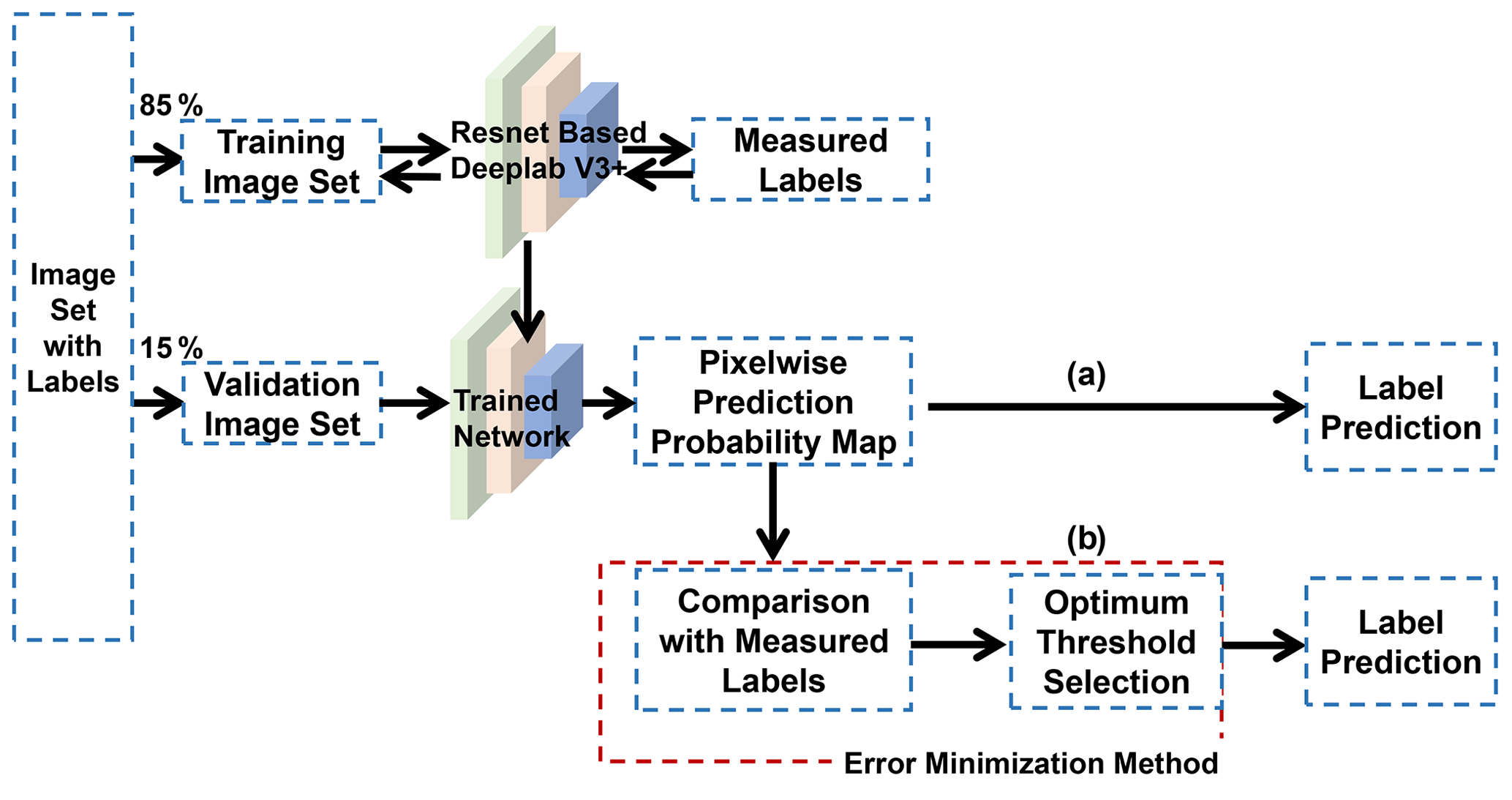
Figure 4 illustrates our general workflow to train and validate the CNN. As discussed in the next section, we introduced a new method to minimize false positives and improve CNN predictions.
3.1 Raw CNN prediction for water
We evaluated the performance of the trained CNN by comparing the number of predicted water pixels to those “measured” as water in the validation set (also called “ground truth”).
Following semantic segmentation, each pixel (i,j) was assigned a probability to belong to water (k= “w”), sky (k= “s”), or background (k= “b”), with the dominant class being the one with highest probability. Thus, water pixels were described by the following binary matrix:
where Θ is the Heaviside function (Θ(x)=0 for x<0 and Θ(x)=1 otherwise). By definition, wij=1 for water pixels and 0 otherwise.
The total number of predicted water pixels in a given picture was then
Similarly, the number of measured water pixels was
where mij is the binary matrix for water obtained from hand annotation and equals 1 for pixels identified as water and 0 otherwise.
As shown in Fig. 5, raw CNN predictions (Ap) compared quite well to the measurements (Am), in particular during flooding conditions. The algorithm handled different lighting conditions well and clearly distinguished water and sky during storms. In general, there were no noticeable radiometric or geometric errors due to saturation, brightness, or hue caused by the Sun or the GoPro curved lens introduced by different camera angles or distance to water.
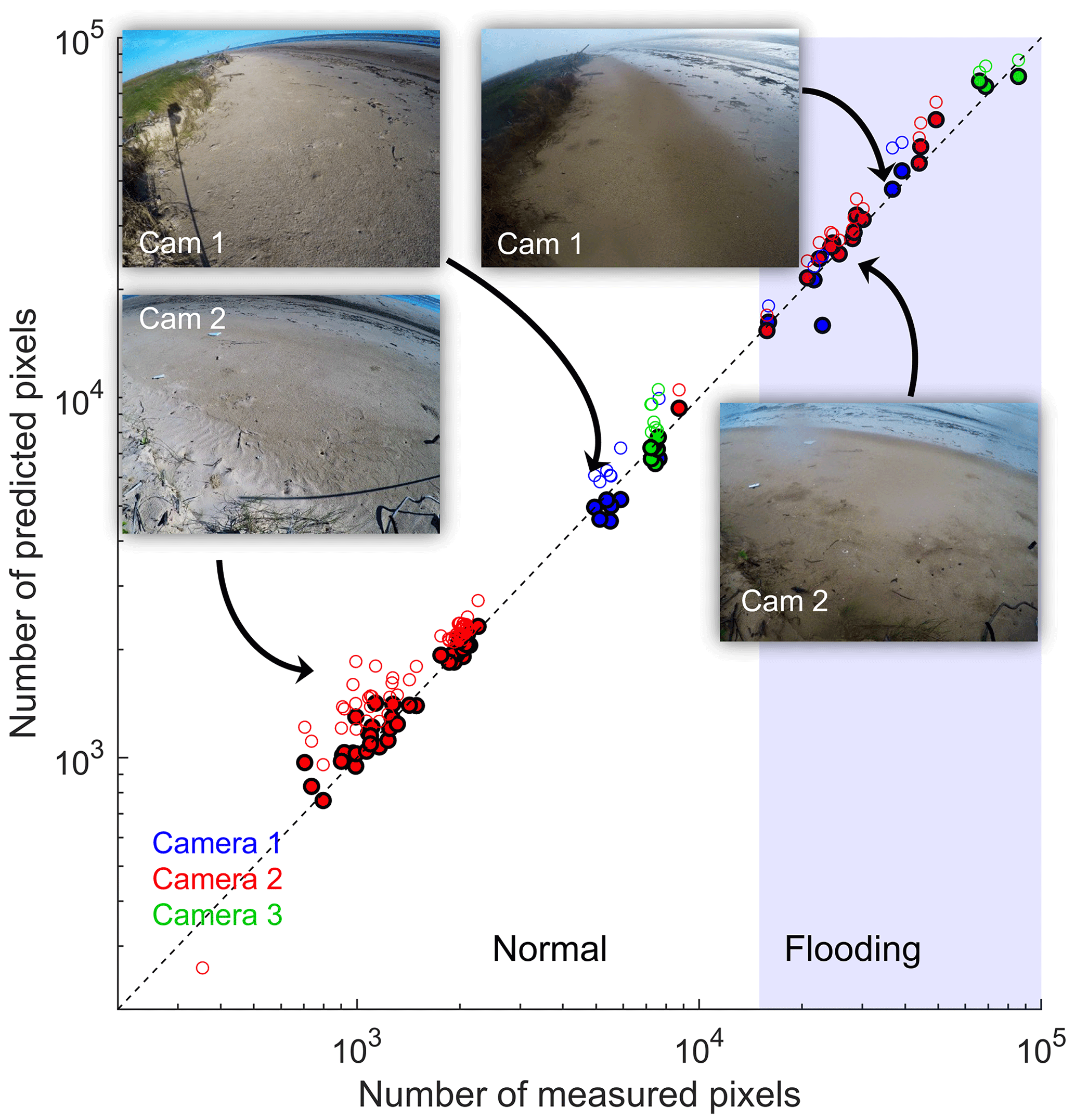
Figure 5Comparison of CNN-predicted and measured water pixels for the 91 pictures in the validation set. The color of the symbol represents the camera used. Both raw CNN predictions (open symbols) and improved ones (filled symbols) are shown. Beach flooding seems to take place when the number of water pixels exceeds 104.
3.1.1 Evaluation of accuracy
We quantified the accuracy of predictions for a single picture using three different metrics. The first one is the “accuracy ratio” defined as the ratio of predicted to measured water pixels:
which just compares the size of the datasets without distinction between false positives or false negatives.
The second one is the true positive rate or “sensitivity”, defined as ratio of the number of true positives, given by the intersection Am∩p of both datasets (i.e., measured water pixels also predicted as water by the CNN), and the number Am of measured water pixels:
where .
By definition, the sensitivity b includes only true positives and therefore measures the effect of false negatives while neglecting false positives. In fact, the fraction of false positives is given by the following difference:
where is the number of false positive pixels.
The third metric is the intersection over union (IoU):
which takes into account both sources of errors: false negatives and false positives.
Instead of analyzing the accuracy for individual images (it will be discussed afterwards), we use the mean absolute percentage error (MAPE) to provide a scale-independent metric of the global CNN performance.
The MAPE is defined as the mean over all images of the absolute deviations of r, b, and u from the ideal value 1:
where N is the total number of images and the subscript n denote values for a single image. Therefore, the MAPEs quantify the deviations of the different accuracy metrics from the ideal, such that a perfect prediction would have MAPEs equal to 0. For simplicity, in what follows we will refer to the MAPE simply as the error of the respective accuracy metric.
We found the general error of the CNN, given by δr and δu, was about 20 %. The CNN was much better at predicting all measured water pixels, with only about 2 % error in the fraction of true positives, as given by δb, which suggests most of the CNN uncertainty comes from false positives. Indeed, the average fraction of false positives () is about 22 %, as some regions have been mislabeled as water instead of background, for example, some frosts, wooden pieces, or wet sand areas near water (Fig. 6). One likely explanation is that the algorithm is trained in a manner that it tries to avoid false negatives while still allowing for false positives.
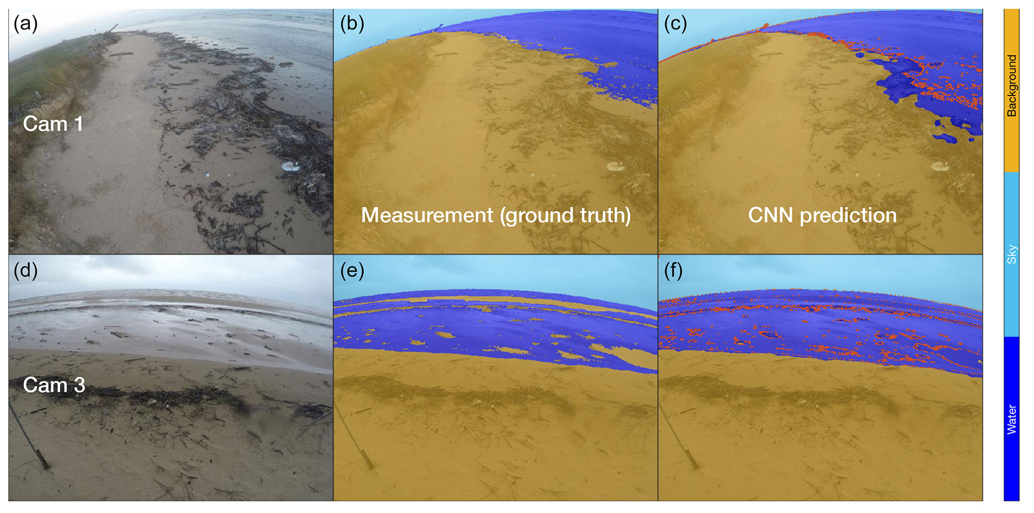
Figure 6Examples of image segmentation during flooding conditions for cameras 1 (a, b, c) and 3 (d, e, f), showing the occurrence of false positives when the CNN mislabels wet sand as water. The red dots superimposed on the CNN prediction on the right panel represents the limits of the actual extension of water measured manually (b, e).
3.2 Improved CNN predictions
Our results demonstrate the utility of using a simple post-processing method to minimize the error δr of the accuracy ratio r by using only the classification probability. Although we focused on water segmentation, the proposed method could be extended further to the prediction of other classes as well. The central idea of such a method is to impose a threshold pt on the predicted water label wij (Eq. 1), such that a given pixel (i,j) is classified as water when the probability is both the highest among the different classes and above pt. The filtered binary matrix for water pixels in this case was given by
From this definition it follows that the number Ap of predicted water pixels and the ratios r, b, and u, as well as their corresponding MAPEs (Eqs. 2 and 4–10), are all a function of the threshold probability pt. Imposing a threshold thus corresponds to a filtering of the raw CNN prediction. A zero threshold (pt=0) gives back the unfiltered values introduced in the previous section.
For threshold probabilities below 0.5, we find the error of the accuracy ratio (δr) remains constant around 20 %, which essentially corresponded to the unfiltered results (Fig. 7). For larger thresholds, δr decreased and reached a minimum of about 7 % for pt≈0.9. Similarly, the error of the IoU (δu) reaches a minimum of about 15 % also for pt≈0.9. In contrast, the error of the sensitivity (δb) consistently increased with pt as more true positives are filtered out (Fig. 7).
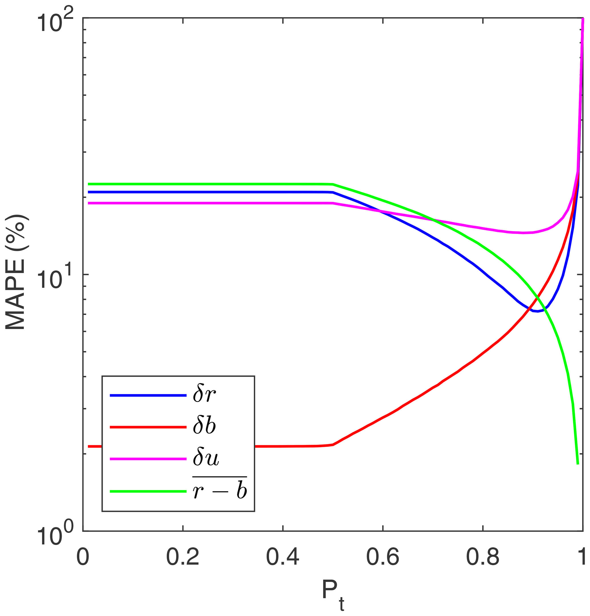
Figure 7Mean absolute percentage errors (MAPE) of the accuracy ratio (δr), the sensitivity (δb), and the intersection over union (δu) as a function of the threshold probability pt. The average fraction of false positives is also shown (in percentage).
The improvement in the accuracy ratio for increasing thresholds, as evidenced by a decrease in the error δr, was mainly due to the consistent reduction of false positives, shown by the average fraction of false positives in Fig. 7. For water thresholds up to 0.9, the reduction of false positives outweighed the decrease in the sensitivity (i.e., higher error δb) led by the decrease of true positives (Fig. 7). However, for thresholds above 0.9, the loss of true positives became dominant and the CNN accuracy worsened as δr increased.
We selected pt=0.9 as the optimum threshold probability for water segmentation in our validation set (Fig. 4), as it provided the most accurate results in terms of both the accuracy ratio and IoU (Fig. 7). Indeed, filtering the CNN results using pt=0.9 noticeably increased the accuracy of the CNN predictions and improved the accuracy ratio across the whole range of water conditions (Fig. 8).
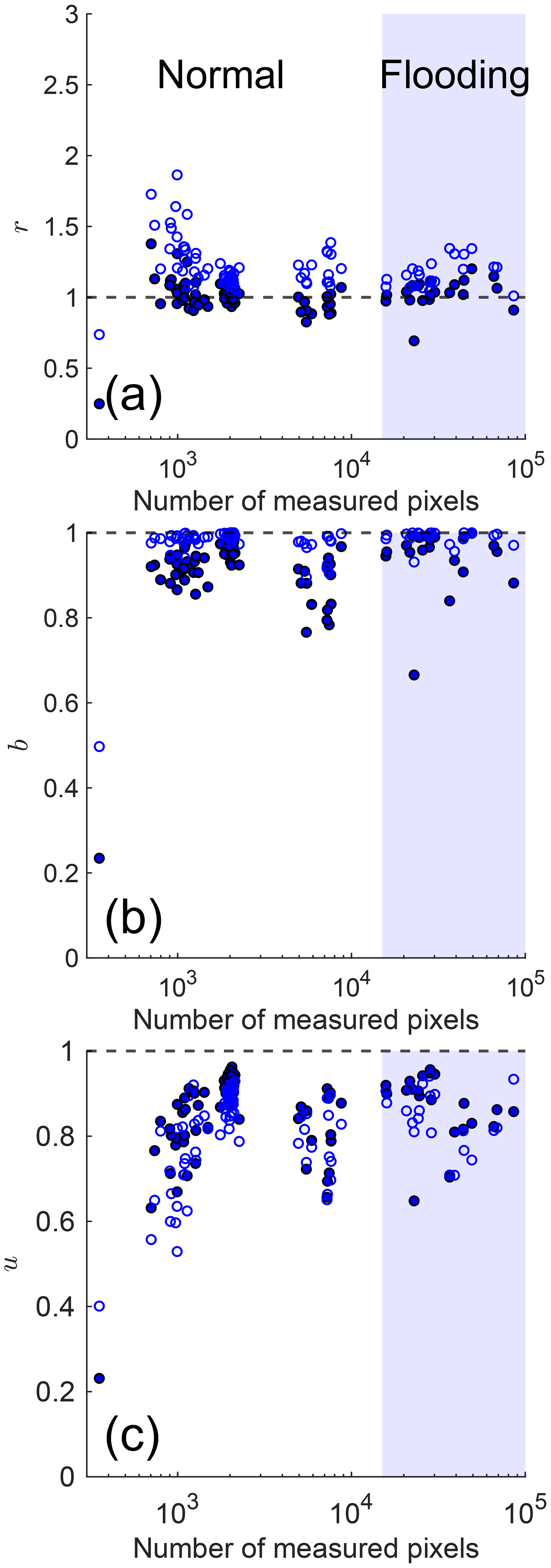
Figure 8(a) Accuracy ratio (r), (b) sensitivity (b), and (c) intersection over union (u) of the CNN predictions for water segmentation of individual images of the validation set as function of the number of measured water pixels. Both raw CNN predictions (pt=0, open symbols) and filtered ones (pt=0.9, filled symbols) are shown.
3.3 Effects of diversity and number of training images
Given how time-consuming the training step can be, we were also interested in understanding how the accuracy of the trained CNN depended on two main factors: the diversity of images in the training set and the number of images in the training set.
Since we were primarily interested in identifying water, we divided the training set into two groups depending on the number of water pixels: “flooding images” with more than 1.5×10⁴ water pixels and “normal images” otherwise (see pictures in Fig. 5). The number of training images was kept constant at 393 for every trained CNN, while the fraction of flooding images was increased from 0 % to about 23 %. Each trained CNN was then tested with the validation set, which has 21 flooding images and 70 normal images.
As expected, the accuracy of the predictions for flooding images in the validation set increased with the proportion of flooding images in the training set, with the error δr quickly decreasing from about 50 % for no flooding images to about 12 % for 23 % of flooding images (Fig. 9). Surprisingly, the accuracy of the predictions for normal images in the validation set also improved by almost 50 % (with δr decreasing from 40 % to about 20 %), despite the decrease in the fraction of normal images in the training set, which led to a significant improvement in the general accuracy of the CNN (Fig. 9). The trend continued up to the point where 23 % of the training set was composed of flooding images. Beyond that, when 26 % of flooding images were included in the training set, we noted a decline in accuracy. Specifically, the error rate δr rose from 20 % to about 27 % for the total validation set and from 22 % to approximately 30 % for normal images. As a result, this revealed a critical threshold in the utilization of flooding images within the training data, highlighting the importance of an optimal balance for effective modeling.
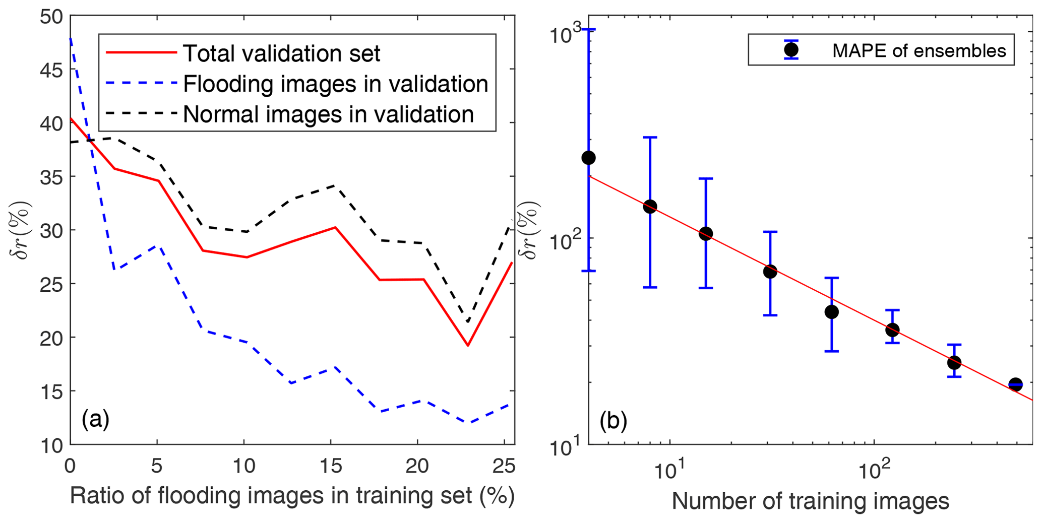
Figure 9The mean absolute percentage error (δr) of the accuracy ratio of CNNs trained with different fractions of flooding images (a) and different number of images (b).
Furthermore, to investigate the effect of the number of training images on CNN accuracy, we trained it using a random subset of N different images from the total of 493 images available for training, roughly doubling N from 4 to 493 (Fig. 9b). For each value N, we repeated the training M times using different random samples to randomize the image type and account for changes in the fraction of flooding images. We chose M=50 for N<100, decreasing M for larger training sets (M=10 and 5 for N=123 and 247, respectively) to save training time. Each of the trained CNNs was then applied to the whole validation set to evaluate its accuracy.
Again, as expected, the accuracy of the predictions increased with the size of the training set (Fig. 9), with a large error δr, in the range 100 %–1000 %, when using only 4 training images, down to about 20 % for the total set of 493 images. We found that δr(N) decreases with , which points to the random nature of the convergence of the CNN prediction.
Our results demonstrate that CNN-based image segmentation is a viable method to identify water in complex coastal imagery. We found the mean absolute percentage error (MAPE) of the accuracy ratio (i.e., the ratio of predicted to measured water pixels) to be about 20 %. This error can be further reduced to about 7 % after applying a novel method for filtering false positives during post-processing. After filtering, we found the MAPE of the true positive rate (sensitivity) to be about 8 %, a value similar to the average ratio of false positives. We also found the accuracy of the filtered CNN predictions to be relatively independent of the amount of water in the images, and it tended to be better for images with a larger fraction of water, corresponding to flooding conditions (Fig. 8). As for the lingering problem of false negatives, it may be better solved by interpolating or extrapolating a line across areas with greatest contrast, thereby connecting true-positive regions.
As expected, the accuracy of the raw CNN predictions depended on the training dataset. The accuracy increased with the number N of training images, with the error decreasing as . In general, more than 100 images were needed to reduce the error below 50 %. Furthermore, the CNN performed much better when we increased the diversity of image types during training. This suggested that there is value in using additional metrics for quantifying image diversity, such as the multiscale structural similarity index measure (MS-SSIM), which evaluates the similarity between two images. For instance, we can ensure diversity in the training set by adding pairs of images with very low MS-SSIM values.
Our work demonstrates the usefulness of in situ camera systems with automatic image segmentation for the observation of beach and back-beach overtopping events at specific locations. This method has the potential to enhance the monitoring of local wave runup, in particular after combining it with photogrammetry and other ways to measure actual spatial data, thus contributing to improve predictions of nuisance coastal flooding and potentially enhancing coastal resilience. Indeed, our findings open the way for the extraction of high temporal resolution data to better understand the stochastic properties of flooding events and validate and/or improve widely used empirical runup formulas. This stochastic analysis and the comparison with empirical predictions is the focus of the second part of this study (Kang et al., 2023a).
The dataset encompassing the trained CNN based on ResNet-18, along with the image dataset and the manual labels, is available in the Texas Data Repository (https://doi.org/10.18738/T8/UYZUBK, Kang et al., 2023b).
ODV designed the study. ODV, RAF, and TH installed the field equipment and carried out the observations. BK performed the CNN-based image segmentation. BK and ODV performed the analysis. BK and ODV prepared the manuscript with contributions from all co-authors.
At least one of the (co-)authors is a member of the editorial board of Earth Surface Dynamics. The peer-review process was guided by an independent editor, and the authors also have no other competing interests to declare.
Publisher's note: Copernicus Publications remains neutral with regard to jurisdictional claims made in the text, published maps, institutional affiliations, or any other geographical representation in this paper. While Copernicus Publications makes every effort to include appropriate place names, the final responsibility lies with the authors.
Orencio Durán Vinent and Byungho Kang were supported by the Texas A&M Engineering Experiment Station.
This paper was edited by Sagy Cohen and reviewed by two anonymous referees.
Alvarez-Ellacuria, A., Orfila, A., Gómez-Pujol, L., Simarro, G., and Obregon, N.: Decoupling spatial and temporal patterns in short-term beach shoreline response to wave climate, Geomorphology, 128, 199–208, https://doi.org/10.1016/j.geomorph.2011.01.008, 2011. a
Battjes, J. A.: Surf Similarity, Coastal Engineering Proceedings, 1, 26, https://doi.org/10.9753/icce.v14.26, 1974. a
Bengio, Y.: Deep Learning of Representations for Unsupervised and Transfer Learning, Proceedings of Machine Learning Research, 27, 17–36, http://proceedings.mlr.press/v27/bengio12a.html (last access: 20 December 2023), 2012. a
Buscombe, D. and Ritchie, A.: Landscape Classification with Deep Neural Networks, Geosciences, 8, 244, https://doi.org/10.3390/geosciences8070244, 2018. a
Chen, L.-C., Papandreou, G., Kokkinos, I., Murphy, K., and Yuille, A. L.: DeepLab: Semantic Image Segmentation with Deep Convolutional Nets, Atrous Convolution, and Fully Connected CRFs, arXiv [preprint], https://doi.org/10.48550/arXiv.1606.00915, 2016. a, b
Chen, L.-C., Papandreou, G., Schroff, F., and Adam, H.: Rethinking Atrous Convolution for Semantic Image Segmentation, arXiv [preprint], https://doi.org/10.48550/arXiv.1706.05587, 2017. a
Chen, L.-C., Zhu, Y., Papandreou, G., Schroff, F., and Adam, H.: Encoder-Decoder with Atrous Separable Convolution for Semantic Image Segmentation, arXiv [preprint], https://doi.org/10.48550/arXiv.1802.02611, 2018. a
den Bieman, J. P., de Ridder, M. P., and van Gent, M. R. A.: Deep learning video analysis as measurement technique in physical models, Coast. Eng., 158, 103689, https://doi.org/10.1016/j.coastaleng.2020.103689, 2020. a
Eigen, D. and Fergus, R.: Predicting Depth, Surface Normals and Semantic Labels with a Common Multi-Scale Convolutional Architecture, arXiv [preprint], https://doi.org/10.48550/arXiv.1411.4734, 2014. a
Hallegatte, S., Green, C., Nicholls, R. J., and Corfee-Morlot, J.: Future flood losses in major coastal cities, Nat. Clim. Change, 3, 802–806, https://doi.org/10.1038/nclimate1979, 2013. a
Hinton, G. E., Osindero, S., and Teh, Y.-W.: A fast learning algorithm for deep belief nets, Neural Comput., 18, 1527–1554, https://doi.org/10.1162/neco.2006.18.7.1527, 2006. a
Holman, R. and Guza, R.: Measuring run-up on a natural beach, Coast. Eng., 8, 129–140, https://doi.org/10.1016/0378-3839(84)90008-5, 1984. a
Holman, R. and Stanley, J.: The history and technical capabilities of Argus, Coast. Eng., 54, 477–491, https://doi.org/10.1016/j.coastaleng.2007.01.003, 2007. a
Hoonhout, B. M., Radermacher, M., Baart, F., and van der Maaten, L. J. P.: An automated method for semantic classification of regions in coastal images, Coast. Eng., 105, 1–12, https://doi.org/10.1016/j.coastaleng.2015.07.010, 2015. a
Huff, T. P., Feagin, R. A., and J., F.: Enhanced tide model: Improving tidal predictions with integration of wind data, Shore & Beach, 88, 40–45, https://doi.org/10.34237/1008824, 2020. a
Ioffe, S. and Szegedy, C.: Batch Normalization: Accelerating Deep Network Training by Reducing Internal Covariate Shift, arXiv [preprint], https://doi.org/10.48550/arXiv.1502.03167, 2015. a
Kang, B., Feagin, R. A., Huff, T., and Durán Vinent, O.: Stochastic properties of coastal flooding events – Part 2: Probabilistic analysis, EGUsphere [preprint], https://doi.org/10.5194/egusphere-2023-238, 2023a. a
Kang, B.: Trained CNN, Coastal Imagery Dataset, and Manual Labels for Flooding Detection, Texas Data Repository [data set], https://doi.org/10.18738/T8/UYZUBK, 2023b.
LeCun, Y., Boser, B., Denker, J. S., Henderson, D., Howard, R. E., Hubbard, W., and Jackel, L. D.: Backpropagation Applied to Handwritten Zip Code Recognition, Neural Comput., 1, 541–551, https://doi.org/10.1162/neco.1989.1.4.541, 1989. a
Long, J., Shelhamer, E., and Darrell, T.: Fully convolutional networks for semantic segmentation, in: 2015 IEEE Conference on Computer Vision and Pattern Recognition (CVPR), Boston, 7–12 June 2015, 3431–3440, https://doi.org/10.1109/CVPR.2015.7298965, 2015. a
Moftakhari, H. R., AghaKouchak, A., Sanders, B. F., Allaire, M., and Matthew, R. A.: What Is Nuisance Flooding? Defining and Monitoring an Emerging Challenge, Water Resour. Res., 54, 4218–4227, https://doi.org/10.1029/2018WR022828, 2018. a
Moore, F. C. and Obradovich, N.: Using remarkability to define coastal flooding thresholds, Nat. Commun., 11, 530, https://doi.org/10.1038/s41467-019-13935-3, 2020. a
Muhadi, N. A., Abdullah, A. F., Bejo, S. K., Mahadi, M. R., and Mijic, A.: Deep Learning Semantic Segmentation for Water Level Estimation Using Surveillance Camera, Appl. Sci., 11, 9691, https://doi.org/10.3390/app11209691, 2021. a
Nair, V. and Hinton, G. E.: Rectified linear units improve restricted boltzmann machines, Proceedings of the 27th International Conference on International Conference on Machine Learning, Haifa, Israel, 21–24 June 2010, 807–814, https://dl.acm.org/doi/10.5555/3104322.3104425 (last access: 20 December 2023), 2010. a
Nicholls, R. J., Marinova, N., Lowe, J. A., Brown, S., Vellinga, P., De Gusmão, D., Hinkel, J., and Tol, R. S. J.: Sea-level rise and its possible impacts given a “beyond 4 ∘C world” in the twenty-first century, Philos. T. R. Soc. A, 369, 161–181, https://doi.org/10.1098/rsta.2010.0291, 2011. a
Palmsten, M., Birchler, J. J., Brown, J. A., Harrison, S. R., Sherwood, C. R., and Erikson, L. H.: Next-generation tool for digitizing wave runup, in: AGU Fall Meeting Abstracts, Vol. 2020, EP051–10, https://agu.confex.com/agu/fm20/meetingapp.cgi/Paper/757086 (last access: 20 December 2023), 2020. a
Russakovsky, O., Deng, J., Su, H., Jonathan, Ma, S., Huang, Z., Karpathy, A., Khosla, A., Bernstein, M., Alexander, and Fei-Fei, L.: ImageNet Large Scale Visual Recognition Challenge, arXiv [preprint], https://doi.org/10.48550/arXiv.1409.0575, 2015. a
Sáez, F. J., Catalán, P. A., and Valle, C.: Wave-by-wave nearshore wave breaking identification using U-Net, Coast. Eng., 170, 104021, https://doi.org/10.1016/j.coastaleng.2021.104021, 2021. a
Stockdon, H. F., Holman, R. A., Howd, P. A., and Sallenger, A. H.: Empirical parameterization of setup, swash, and runup, Coast. Eng., 53, 573–588, https://doi.org/10.1016/j.coastaleng.2005.12.005, 2006. a
Stockdon, H. F., Thompson, D. M., Plant, N. G., and Long, J. W.: Evaluation of wave runup predictions from numerical and parametric models, Coast. Eng., 92, 1–11, https://doi.org/10.1016/j.coastaleng.2014.06.004, 2014. a
Strauss, B. H., Ziemlinski, R., Weiss, J. L., and Overpeck, J. T.: Tidally adjusted estimates of topographic vulnerability to sea level rise and flooding for the contiguous United States, Environ. Res. Lett., 7, 014033, https://doi.org/10.1088/1748-9326/7/1/014033, 2012. a
Valentini, N. and Balouin, Y.: Assessment of a Smartphone-Based Camera System for Coastal Image Segmentation and Sargassum monitoring, Journal of Marine Science and Engineering, 8, 23, https://doi.org/10.3390/jmse8010023, 2020. a
Vandaele, R., Dance, S. L., and Ojha, V.: Deep learning for automated river-level monitoring through river-camera images: an approach based on water segmentation and transfer learning, Hydrol. Earth Syst. Sci., 25, 4435–4453, https://doi.org/10.5194/hess-25-4435-2021, 2021. a
Vitousek, S., Barnard, P. L., Fletcher, C. H., Frazer, N., Erikson, L., and Storlazzi, C. D.: Doubling of coastal flooding frequency within decades due to sea-level rise, Sci. Rep.-UK, 7, 1399, https://doi.org/10.1038/s41598-017-01362-7, 2017. a, b
Vousdoukas, M. I., Ferreira, P. M., Almeida, L. P., Dodet, G., Psaros, F., Andriolo, U., Taborda, R., Silva, A. N., Ruano, A., and Ferreira, O. M.: Performance of intertidal topography video monitoring of a meso-tidal reflective beach in South Portugal, Ocean Dynam., 61, 1521, https://doi.org/10.1007/s10236-011-0440-5, 2011. a
Wilson, A. C., Roelofs, R., Stern, M., Srebro, N., and Recht, B.: The Marginal Value of Adaptive Gradient Methods in Machine Learning, arXiv [preprint], https://doi.org/10.48550/arXiv.1705.08292, 2017. a
Yu, F. and Koltun, V.: Multi-Scale Context Aggregation by Dilated Convolutions, arXiv [preprint], https://doi.org/10.48550/arXiv.1511.07122, 2015. a