the Creative Commons Attribution 4.0 License.
the Creative Commons Attribution 4.0 License.
 | 10 Jan 2024
Stochastic properties of coastal flooding events – Part 2: Probabilistic analysis
Byungho Kang
Rusty A. Feagin
Thomas Huff
Orencio Durán Vinent
Low-intensity but high-frequency coastal flooding, also known as nuisance flooding, can negatively affect low-lying coastal communities with potentially large socioeconomic effects. Partially driven by wave runup, this type of flooding is difficult to predict due to the complexity of the processes involved. Here, we present the results of a probabilistic analysis of flooding events measured on an eroded beach at the Texas coast. A high-resolution time series of the flooded area was obtained from pictures using convolutional neural network (CNN)-based semantic segmentation methods, as described in the first part of this contribution. After defining flooding events using a peak-over-threshold method, we found that their size follows an exponential distribution. Furthermore, consecutive flooding events were uncorrelated at daily timescales but correlated at hourly timescales, as expected from tidal and day–night cycles. Our measurements confirm the broader findings of a recent multi-site investigation of the probabilistic structure of high-water events that used a semi-empirical formulation for wave runup. Indeed, we found a relatively good statistical agreement between our CNN-based empirical flooding data and predictions using total-water-level estimations. As a consequence, our work supports the validity of a relatively simple probabilistic model of high-frequency coastal flooding driven by wave runup that can be used in coastal risk management and landscape evolution models.
- Article
(4882 KB) - Full-text XML
- Companion paper
- BibTeX
- EndNote


Coastal flooding is induced by a short-term rise in water levels caused by a mix of stochastic and deterministic events, such as storm surges, wave runup, tides or river discharge due to heavy precipitation (Muis et al., 2016; Ward et al., 2018; Bevacqua et al., 2019). In addition to extreme hurricane-driven flooding events with return periods on the order of 10 or more years, the importance of low-intensity high-frequency flooding events, with return periods on the order of months, has recently became clear (Sweet et al., 2014; Moftakhari et al., 2017, 2018). When accumulated over time, the social cost of nuisance flooding can outweigh the costs from the large-scale flooding (Moftakhari et al., 2017, 2018). This low-intensity flooding also controls the formation and post-storm recovery of coastal dunes, which are essential for the stability of barrier islands (Durán Vinent et al., 2021).
High-frequency and low-intensity coastal flooding is mostly driven by extreme values of wave runup superimposed to the tidal signal (Serafin and Ruggiero, 2014; Serafin et al., 2017) overtopping a characteristic beach elevation, or any other feature close to the shoreline. As the characteristic elevation of natural beaches typically adjusts to the average wave runup during high tide, they are only flooded during extreme events (Rinaldo et al., 2021). Therefore, it is very difficult to predict in detail and has to be described statistically. This probabilistic description can ideally lead to the estimation of both the overtopping frequency λ(Z) (or return period ) of a given elevation Z and the average size of events overtopping Z. This information can then be used to assess the vulnerability of coastal features and coastal infrastructure and plan accordingly.
Recently, Rinaldo et al. (2021) investigated the stochastic properties of high-water events (HWEs), which are associated with coastal flooding, at several locations in the US and across the world. These events were defined as clusters of consecutive days when total water levels exceeded a given threshold. The total water level was calculated by adding still water level data, containing tides and surges, to predicted wave runup data. Wave runup was estimated empirically as function of the deep-water significant wave height and wavelength (Stockdon et al., 2006, 2014). They found that HWEs overtopping a characteristic beach elevation (and thus leading to coastal flooding) were uncorrelated and occurred randomly in time and can thus be modeled as a Poisson process. They also found that their size, defined as the maximum total water level during the event relative to the beach elevation, follows an exponential distribution. These findings can be summarized in an equation for the overtopping frequency of a threshold elevation Z: , where λb=18 yr−1, is the site-dependent average size of HWEs ( m) and Zr is a reference elevation that depends on the tidal amplitude and average wave runup and can be interpreted as a characteristic beach elevation (Rinaldo et al., 2021).
However, in spite of the generality and simplicity of the Rinaldo et al. (2021) results, they were based on empirically estimated wave runup data, and therefore it is not clear how they compare to direct measurements of coastal flooding.
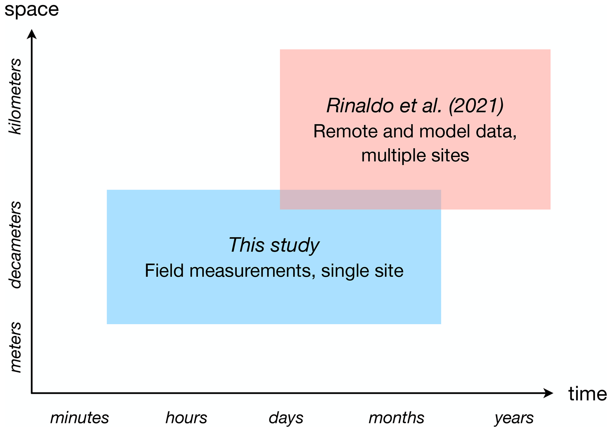
The primary goal of the present study is to describe the probabilistic structure of flooding events measured at a recently eroded site in northern Texas. Flooding events were defined applying the peak-over-threshold method to a high-resolution time series of water area fraction, obtained from coastal images using convolutional neural network (CNN)-based image segmentation as explained in Part 1 of this work (Kang et al., 2024). A central outcome of our research is the validation of the results of Rinaldo et al. (2021). As shown in Fig. 1, although our study complements the spatial and temporal range investigated by Rinaldo et al. (2021), it is limited to a single site and roughly half-year data. However, we can use our results to establish the validity of the more general predictions of Rinaldo et al. (2021).
In what follows we introduce and correct the time series of water data, define flooding events, perform the statistical analysis of both the size and inter-arrival of flooding events, and compare it to the results of Rinaldo et al. (2021). We finalize with a presentation of the probabilistic model for low-intensity and high-frequency coastal flooding events summarizing both our results and those of Rinaldo et al. (2021).
2.1 Field data
As explained in Kang et al. (2024), we installed three solar-powered stationary GoPro cameras, each with a different field of view, on a beach near Cedar Lakes, Texas, to monitor the recovery after Hurricane Harvey in 2017 completely eroded the coastal dunes and the back-beach region (see Fig. 2). This site was subject to frequent wave runup events due to its low-lying bathymetric–topographic profile. Each camera captured pictures every 5 min during a 06:00–18:00 LT. observation period and turned off automatically during the night. From November 2017 to May 2018, we captured more than 51 000 images.
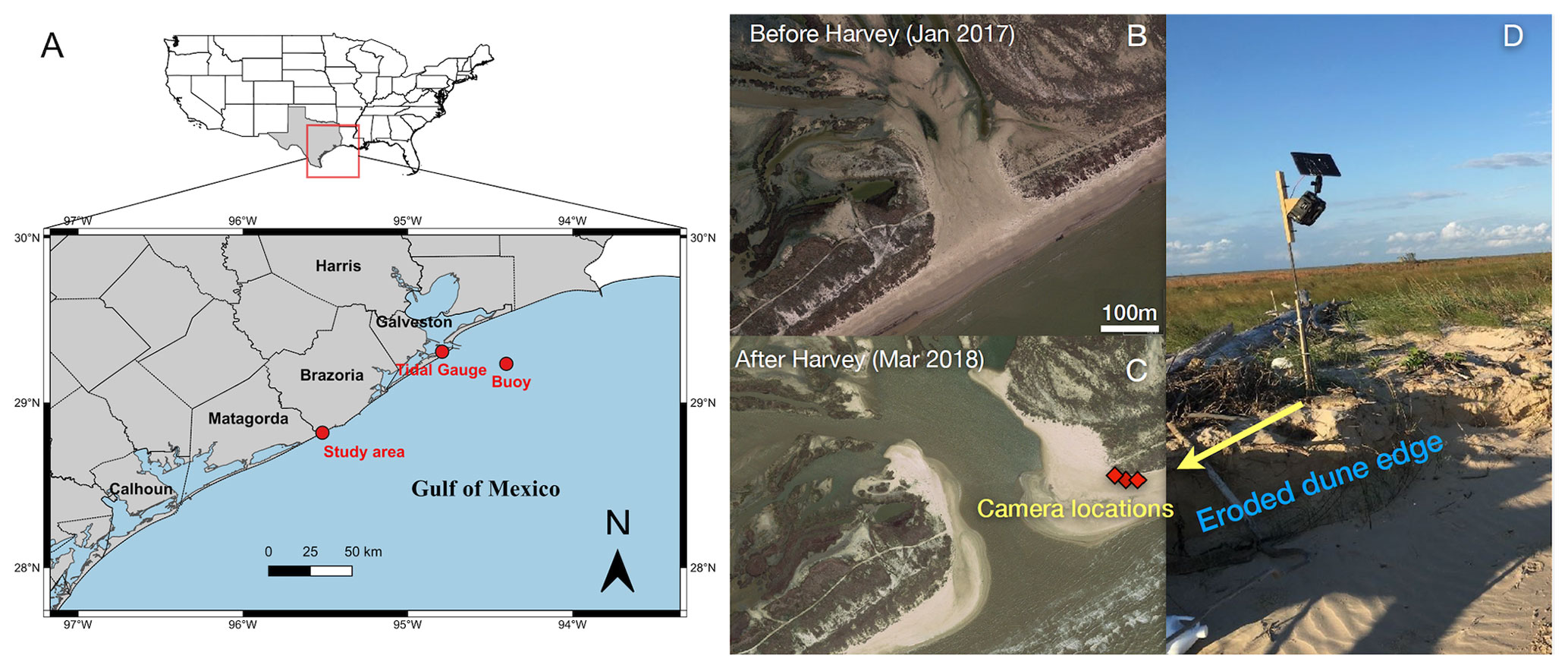
Figure 2Location of field observations (a). Three solar-powered cameras (b–d) were installed in Cedar Lakes, Texas, a site breached during Hurricane Harvey in 2017 that experiences frequent wave runup flooding. (b, c) Map data are sourced © Google and Landsat/Copernicus.
2.2 Time series of water area fraction
In Kang et al. (2024), we applied CNN-based image segmentation to identify water pixels with an accuracy of more than 90 %. Here we used the CNN to generate a time series of the number of water pixels from 24 793 consecutive non-overlapping daylight pictures, while filling the non-observation periods with zeros. For convenience, the number of water pixels was normalized by the total number of pixels in an image to obtain a water area fraction (Fig. 3).
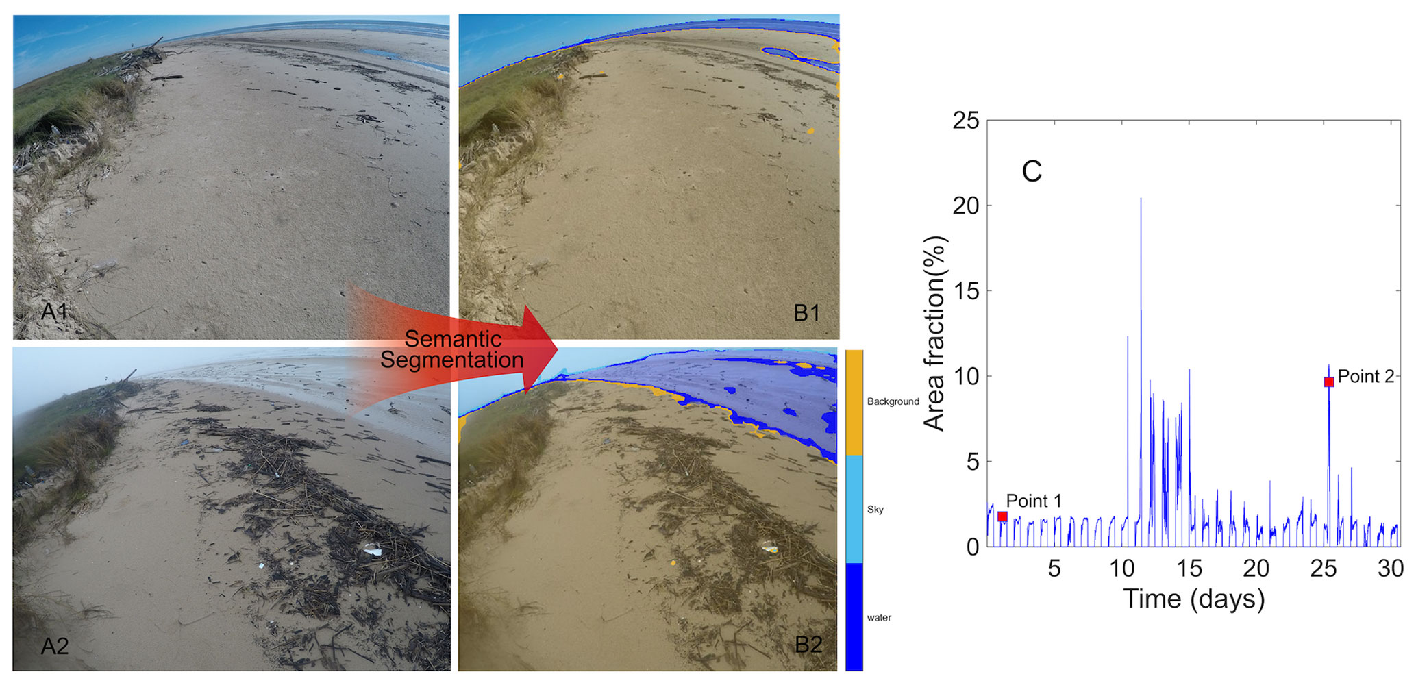
Figure 3(a) Examples of non-flooding and flooding images captured from the camera. Two points at 26 November 2017, 17:29 LT (point 1), and 4 December 2017, 16:49 LT (point 2), are selected to illustrate the area fraction extraction process. (b) Results of the semantic segmentation using the convolutional neural network to identify water, sky and background regions. (c) Time series of the water area fraction, defined as the fraction of water-labeled pixels in the water region of a segmented image (dark blue region in b), from 23 November to 23 December 2017.
Since our observation period was about 6 months, we ignored the effect of seasonality and only corrected the images to account for minor camera rotations due to strong winds and a change in position following one camera replacement (Fig. 4a). These changes in the camera field of view led to different base levels of water area fraction during non-flooding conditions (Fig. 4a). We identified this base level as the most probable value of the water area between camera rotations (or replacements) and estimated it from the mode of the water area distribution during that time period (Fig. 5). We then subtracted the base level (horizontal lines in Fig. 4a) from the area fraction to obtain the excess water area fraction A(t) (Fig. 4b). For simplicity, in what follows we refer to A(t) as simply the water area fraction or just water area.
In order to study the stochastic properties of flooding events at different timescales, we defined a new time series of water area A|τ(t) at timescale τ by taking the maximum of A(t) over a time window τ. For example, A|1 h corresponds to an hourly time series and A|24 h to a daily time series. Note that, by definition, A|5 min is equivalent to A(t) as pictures were taken every 5 min.
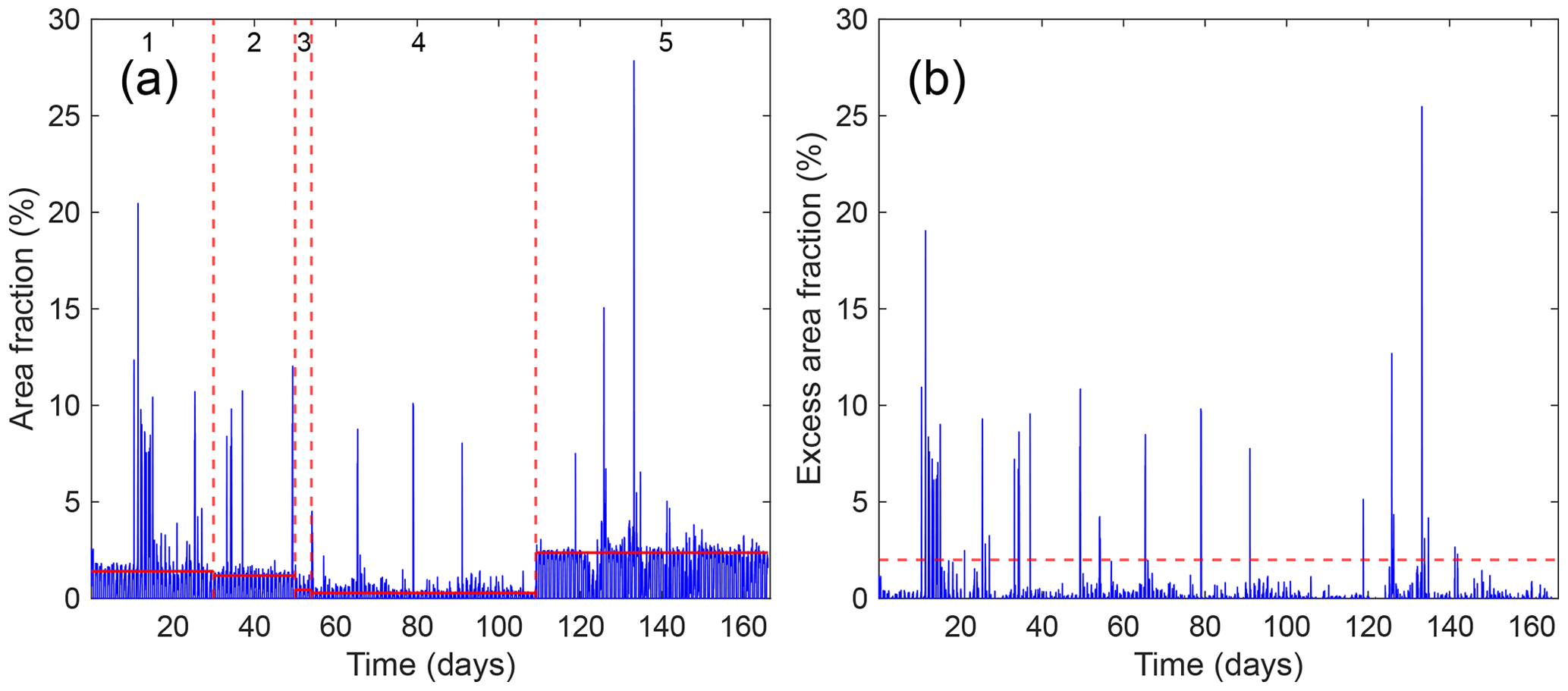
Figure 4(a) Time series of original water area fraction. Dashed lines indicate camera rotations and replacement times dividing the time series into five time spans with a relatively stable field of view. Solid lines show the “base level” for each time segment. (b) Time series of the excess water area fraction A(t) obtained by subtracting the base level in (a) from the area fraction (negative values were neglected). The dashed line shows the selected 2 % threshold separating the extreme values, characterizing flooding conditions from non-flooding conditions.
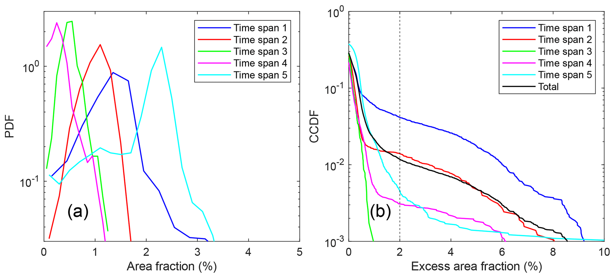
Figure 5(a) Probability density function (PDF) of water area fractions for each time span between camera rotations and/or replacements (see Fig. 4a). The “base level” of the water area fraction shown in Fig. 4a corresponds to the mode of the PDFs for each time span. (b) Complementary cumulative distribution function (CCDF) of the excess area fraction, defined as the area fraction minus the base level (see Fig. 4b), where the 2 % threshold (dashed line) separates the tail, or extreme values associated with coastal flooding, from the bulk. CCDF(A) quantifies the probability of having an excess area fraction larger than A.
2.3 Definition of flooding events
We defined a flooding event as the set of consecutive values of the water area fraction A|τ(t) that exceeded the 2 % threshold (Fig. 6). This threshold allowed a clear separation between typical fluctuations in water area and the extreme values that characterize flooding conditions (Fig. 5b) and can be associated with a characteristic beach elevation above the shoreline. From the definition, flooding events depend on the time window τ, as it is enough for the water area to be above 2 % for a few minutes to count as a threshold crossing at any larger timescale (see Fig. 6).
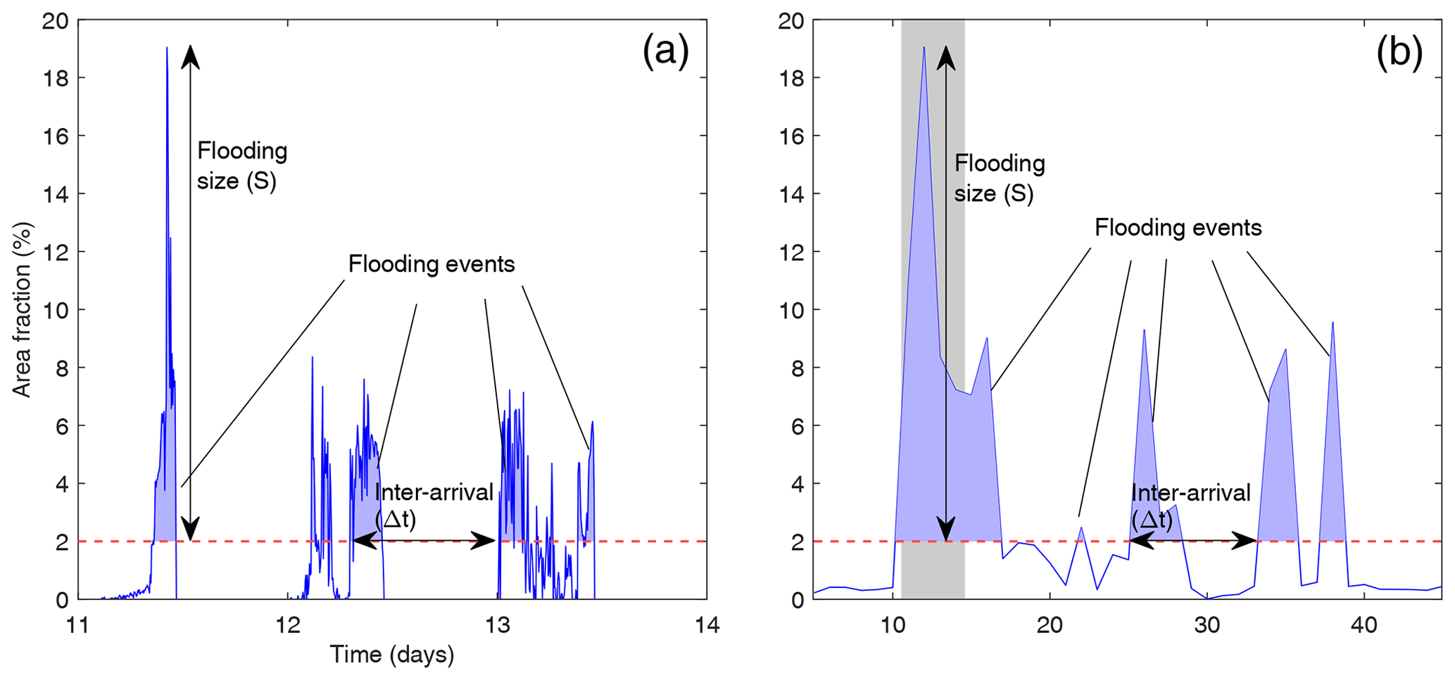
Figure 6Definition of the flooding events, their size (S) and inter-arrivals (Δt) from the excess water area fraction A(t). Examples shown are for the original timescale τ=5 min (a) and for a daily timescale (τ=24 h) (b). Note all the events shown in (a) were clustered in a single event in (b) (shaded region).
Following Rinaldo et al. (2021), we characterized a flooding event i (for a given τ) by its starting time ti, i.e., the time water area increased above 2 %; its duration di; and its size Si, defined as the maximum water area relative to the 2 % threshold during the duration of the event (Fig. 6). Furthermore, we defined the inter-arrival time Δti as the time between consecutive flooding events . Below, we analyze the probability distribution function of the duration d, size S and inter-arrival time Δt of flooding events at different timescales τ.
3.1 Duration of flooding events
At the lowest timescale (and higher time resolution, τ=5 min), the probability density function f(d) of the duration d of flooding events lasting up to 2 h can be approximated by a power law distribution (Fig. 7),
with β=0.7 and a lower limit of dmin=3 min. The fact that this lower limit is below the 5 min temporal resolution of our data suggests that we are missing many relatively short flooding events. Interestingly, as can be seen in Fig. 8, short flooding events are not necessarily of small size.
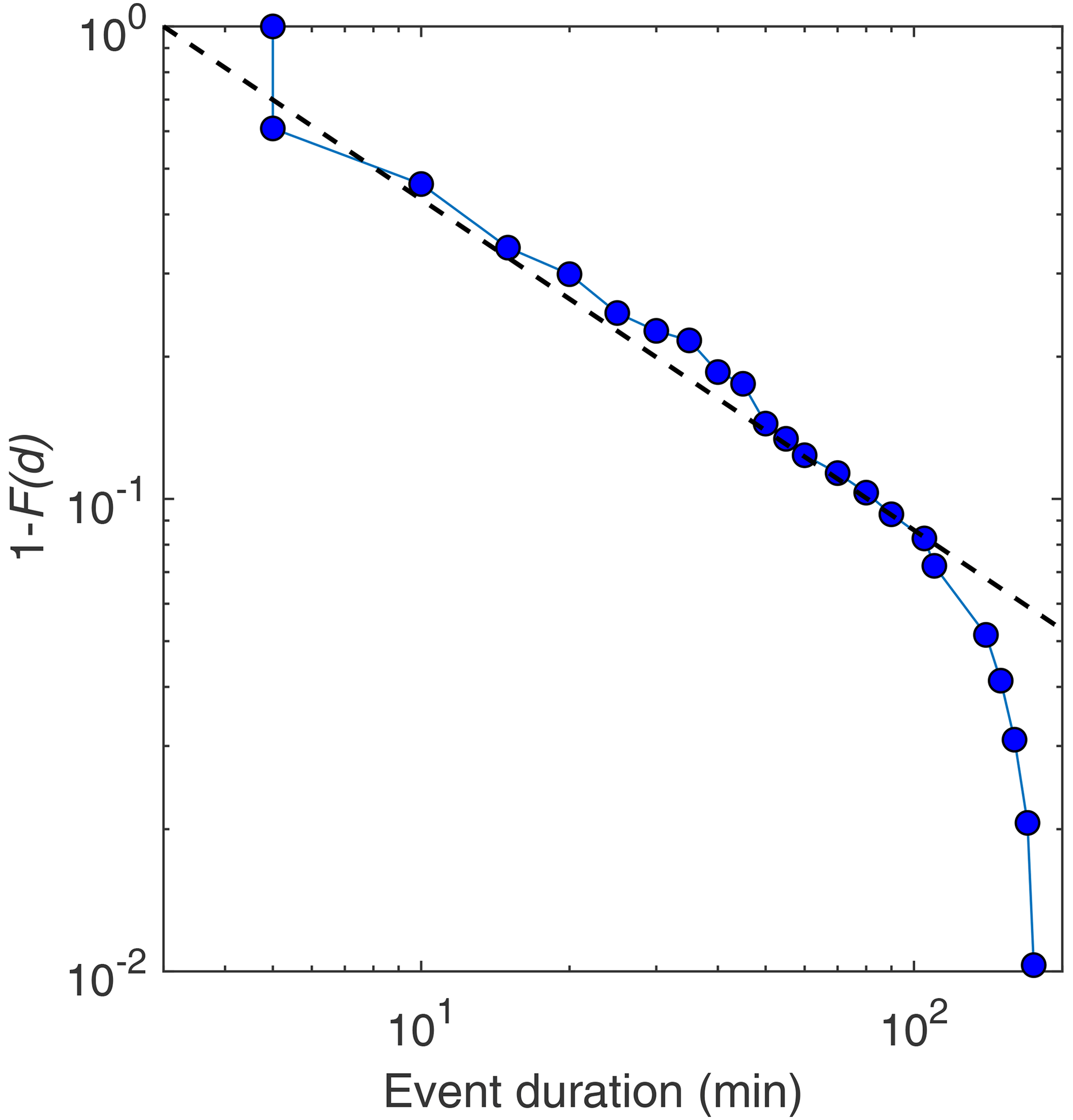
Figure 7Complementary cumulative distribution function 1−F(d) (F is the cumulative distribution function) of the duration d of flooding events. The line shows a power law fit , with exponent β=0.7 and a lower limit dmin=3 min. The time resolution of the data sets a lower cutoff at d=5 min.
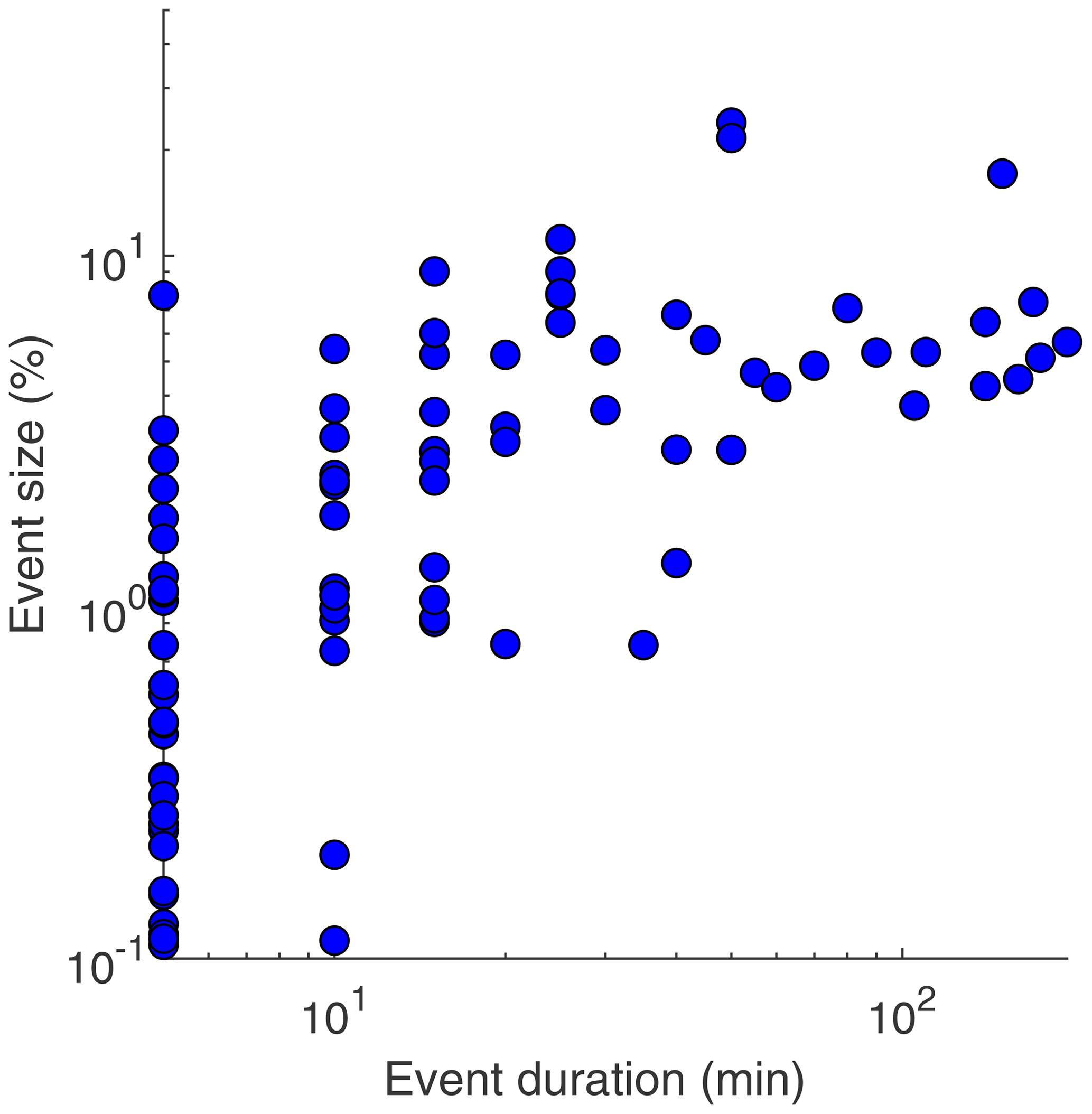
Figure 8Relation between the size S and duration d of flooding events. Note that the event size S is defined as the maximum value of the water area fraction during the event relative to the 2 % threshold. The time resolution of the data is 5 min.
Above 2 h, the event duration data drastically deviated from the power law distribution, with no event lasting more than 3 h in our nearly 6-month-long measurement period (Fig. 7). Furthermore, the size and duration of flooding events was poorly correlated (Fig. 8), as events where water covered around 10 % of the images' pixels (above the 2 % threshold), i.e., S>10 %, can last anywhere from 10 min to 2 h. However, there seems to be a lower limit for the size of events lasting more than 10 min (Fig. 8).
3.2 Distribution of flooding size
The distribution of the size S of flooding events at the lowest timescale (τ=5 min), obtained from A|5 min(t), is well approximated by an exponential distribution with average flooding size % (Fig. 9a). As shown in Fig. 9b, the flooding size distribution remains exponential for timescales τ up to the maximum value investigated (36 h), with p`values higher than the rejection threshold for both the Lilliefors and the Cramér–von Mises tests of exponential fit (Lilliefors, 1969; Cramér, 1928). The average flooding size increases with the timescale τ but seems to saturate to ∼8 % at daily or larger timescales (Fig. 9c).
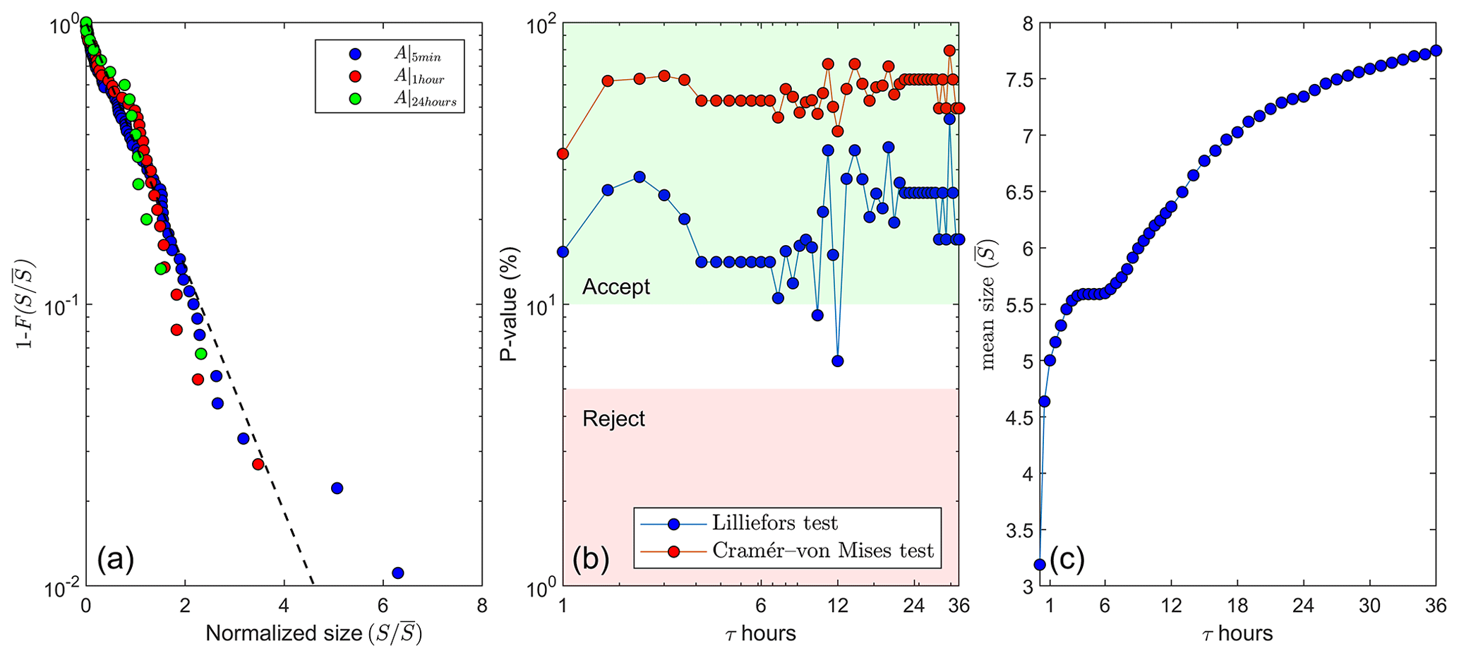
Figure 9(a) Complementary cumulative distribution function of the flooding event size S normalized by the average at three different timescales: τ=5 min, 1 and 24 h. The exponential distribution is shown for reference (dashed line). (b) The p value testing compatibility with the exponential distribution at different timescales (τ) – 0 % (100 %) indicates perfect incompatibility (compatibility) with 5 % as the typical threshold for passing the test. (c) The average size of during flooding events (%) for different timescales τ.
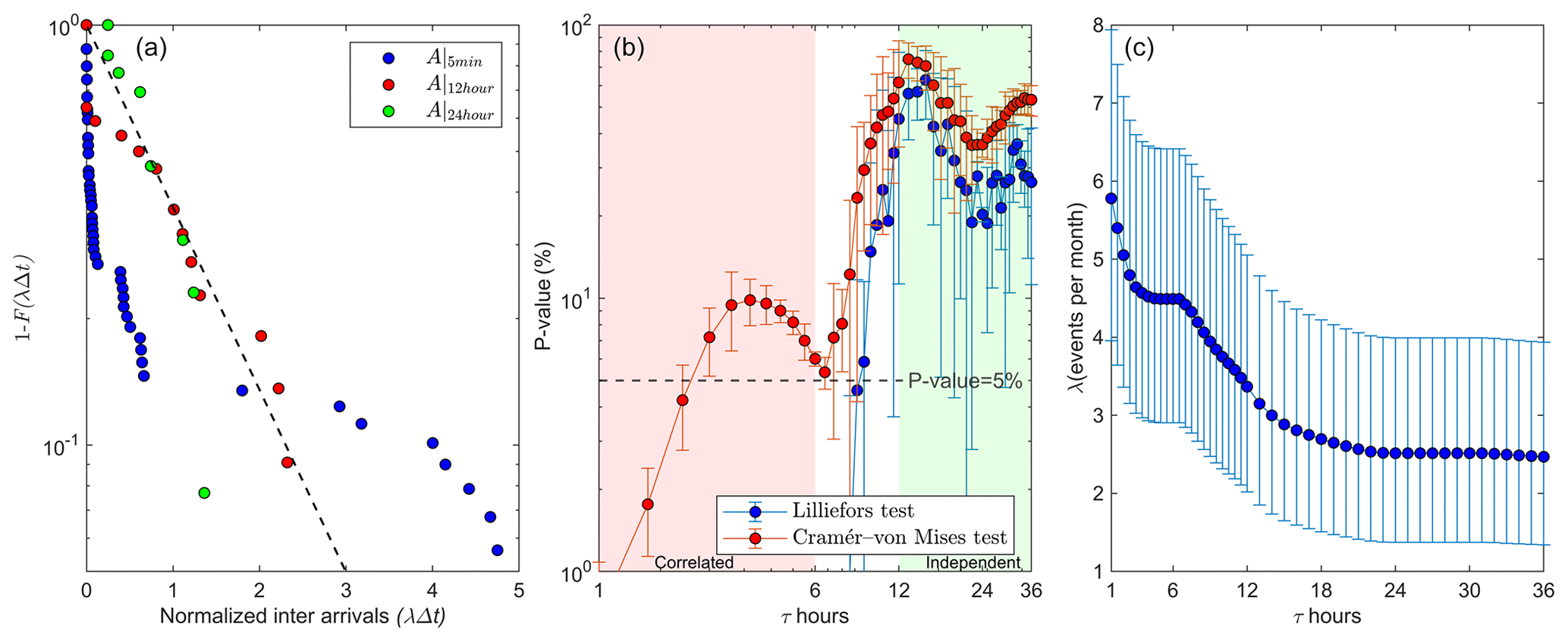
Figure 10(a) Complementary cumulative distribution function 1−F(λΔt) of the inter arrivals (Δt) of flooding events normalized by the flooding frequency at timescales τ=5 min, 12 and 24 h. The exponential distribution is shown for reference (dashed line). (b) Mean p values with confidence-bound (±σ) testing compatibility with the exponential distribution at different timescales (τ) – 0 % (100 %) indicates perfect incompatibility (compatibility) with 5% as the typical threshold for passing the test. Passing the test, i.e., inter-arrivals are exponentially distributed, means the events are independent, whereas failing the test suggests the events are correlated. (c) Frequency λ of flooding events at different timescales (τ), including the 95 % confidence interval obtained by , where and .
3.3 Distribution of inter-arrivals
The distribution of inter-arrivals Δt strongly depends on the timescale τ and seems to converge towards an exponential distribution for timescales above ∼10 h (Fig.10a and b). This is evidenced by the sharp increase in the p values of both the Lilliefors and the Cramér–von Mises tests from around 10 % to about 60 % for timescales between 10 and 12 h (Fig.10b). The p values remain above 30 % for larger timescales.
In these statistical tests, the time at which the time window analysis started was changed to avoid biases. For a given timescale τ, we calculated the goodness of the exponential fit n times, where min is the number of possible initial times at which the time window of size τ could start. For example, the statistical tests were conducted only once for A|5 min(t) but 12 times for A|1 h(t) and 288 times for A|24 h(t).
Given that the exponential distribution of inter-arrivals implies the events are random and independent, we interpreted the large deviations from the exponential distribution for timescales less than 10 h as evidence of correlation between consecutive events (Fig. 10b). At larger timescales, consecutive flooding events did become independent (i.e., their inter-arrival followed an exponential distribution) and can be modeled as a Poisson process.
3.4 Frequency of flooding events
The frequency λ of flooding events is by definition the inverse of the average inter-arrival or equivalently , where N is the total number of flooding events obtained from the condition % and T=167 d is the total duration of the time series. As expected, λ decreases with the timescale τ as flooding events are merged, reaching a plateau at the daily scale of 2.5 events per month, from about 6 events per month at the hourly scale (Fig. 10c). Most of the decrease in λ roughly takes place at the transition from correlated to uncorrelated events for timescales between 6 and 12 h (Fig. 10b).
The exponential distribution of both the flooding size S and the inter-arrival Δt of events over timescales above 10 h is in agreement with the findings of Rinaldo et al. (2021) for the size and inter-arrival of events overtopping a characteristic beach elevation (referred to as high-water events or HWEs) obtained from the predicted daily time series of total water levels. However, how do the predictions compare to the measurements beyond these general stochastic properties? In particular, how does the predicted frequency of HWEs compare with the flooding frequency measured from the camera observations? Also, is the predicted flooding from HWEs correlated to flooding measurements at the daily timescale?
Following the methodology from Rinaldo et al. (2021), which involved calculating the hourly time series of total water elevation for the same site using a beach slope of 0.02, we generated a new time series of daily total water levels relative to mean sea level (MSL). This required summing the still water level as measured by a tidal gauge and a semi-empirical estimation of the 2 % exceedance wave run-up. The latter relied on offshore values of the significant wave height and peak wave frequency and the local beach slope (Stockdon et al., 2006, 2014).
Our data sources included the tidal gauge at Galveston Pier 21 (29.31∘ N, 94.793∘ W) and wave buoy station 42035 (29.236∘ N, 94.403∘ W). Both located in Galveston, Texas, they provided hourly measurements of water levels and significant wave heights and peak period. While the water depth of the wave buoy was 15 m, we did not consider reverse shoaling to deeper water, as recommended by Stockdon et al. (2006), to maintain the simplicity of our analysis and directly compare to the results of Rinaldo et al. (2021). Since we did not perform measurements of the beach profile at the study site in the observation period, we assumed the beach slope, which is needed to calculate wave runup, was constant and equal to 0.02 (Rinaldo et al., 2021).
For consistency, we ignored total water level values during non-observation hours of flooding monitoring. We then converted the hourly time series of total water level to a time series of daily maximum total water level ηd by taking the maximum value per day. This removed tidal cycles from the time series. Finally, we defined a high-water event (HWE) as the set of consecutive daily total water levels exceeding a given elevation Zc relative to MSL (Rinaldo et al., 2021). Here, Zc is interpreted as a characteristic beach elevation in which case HWEs represent potential flooding events. Thus, since flooding events and HWEs are equivalent for the purpose of this work, in what follows we will refer to HWEs as “predicted flooding events”, in contrast to the “measured” flooding events obtained from our CNN-based analysis of camera observations.
4.1 Frequency of predicted vs. measured flooding events
As expected, the frequency of predicted flooding events decreased with the characteristic beach elevation Zc, as the number of overtopping events decreased (Fig. 11). The predicted flooding frequency was within the 95 % confidence interval of the measurements for Zc in the range Zc<0.9 m. This upper limit is consistent with the characteristic beach elevation 0.9 m estimated by Rinaldo et al. (2021) using a digital elevation model (DEM) of the area (Fig. 11). In fact, we expect a lower beach elevation at our site following the large beach erosion after Hurricane Harvey in August 2017, in agreement with the trend observed in Fig. 11.
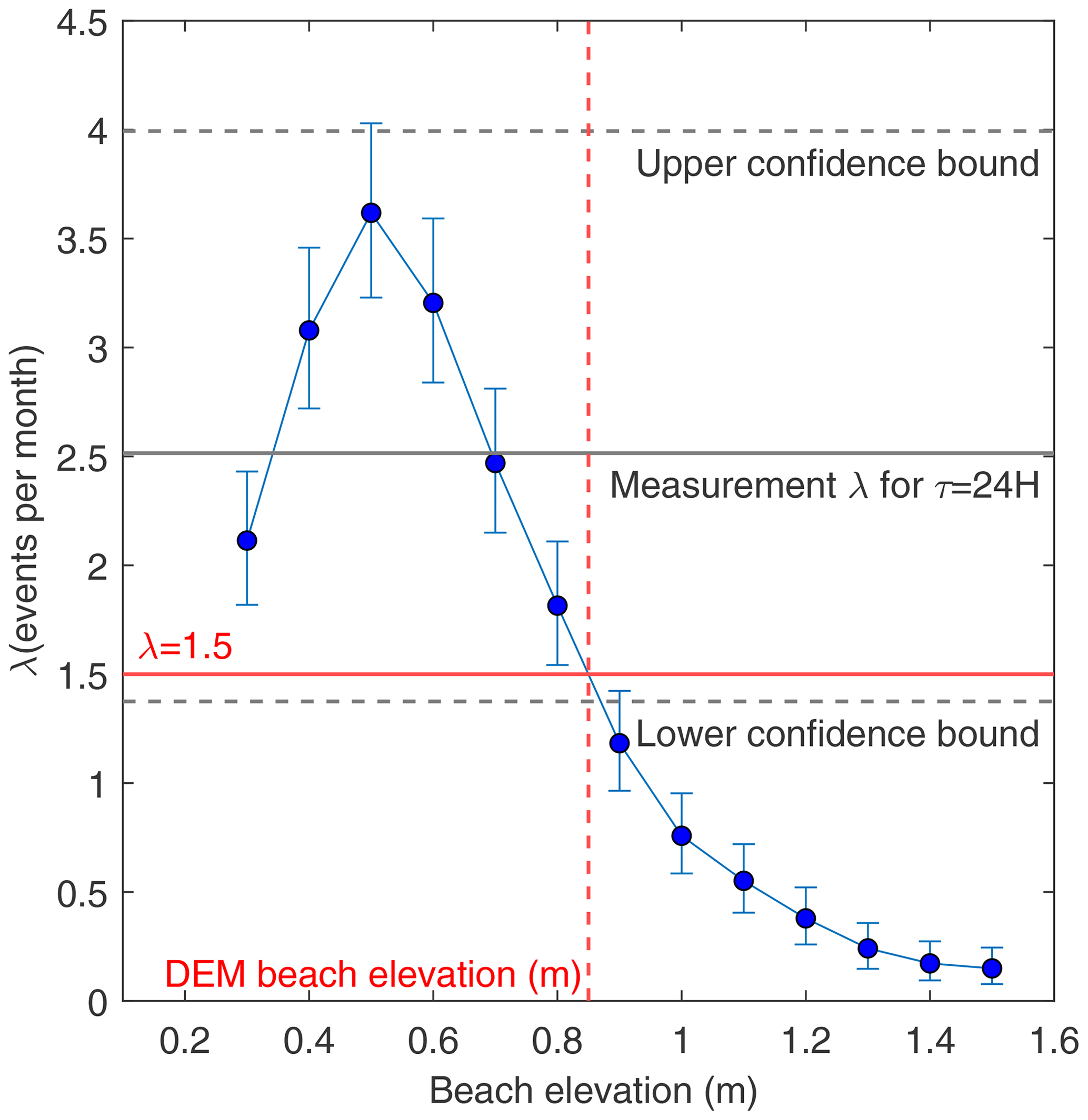
Figure 11Symbols show the frequency (λ) of coastal flooding events predicted by high-water events above a characteristic beach elevation, as a function of the characteristic beach elevation Zc (relative to MSL). The measured frequency (mean ± 95 % confidence interval) of flooding events at the daily timescale is shown for comparison (solid and dashed black lines). The solid red line is the flooding frequency predicted by Rinaldo et al. (2021) for a characteristic beach elevation around 0.9 m (dashed red line) estimated from a digital elevation model (DEM).
Although we lack measurements of the actual beach elevation profile during our observation period, the value Zc=0.7 m, at which the predicted frequency matched the measured value of λ=2.5 per month obtained for a daily timescale (τ=24 h in Fig. 10c), is consistent with the hypothesis that beach erosion can explain potential differences between predicted and measured flooding frequencies. Indeed, the scarp visible at the vegetation edge in Fig. 3a1, is about 20 cm tall and could help explain the elevation gap.
4.2 Synchronicity of measured and predicted flooding events
We also compared flooding predictions to the measurements at the daily level by defining a rescaled daily time series of the measured flooded area fraction (Rm) relative to the 2 % threshold and the predicted water elevation (Rp) above a characteristic beach elevation Zc as follows:
where A|24 h is the excess water area fraction at the daily timescale, 2 % is the threshold for flooding conditions, % is the average size of the measured flooding events for τ=24 h (see Fig. 9c), ηd is the estimated daily maximum of the total water level at the shoreline and m is the average size of the predicted HWEs (Rinaldo et al., 2021). In both cases, the function max ensures Rm and Rp are positive. Due to lack of data, we could only generate predictions for the first 130 d of our total 170 d measurement period (Fig. 12).
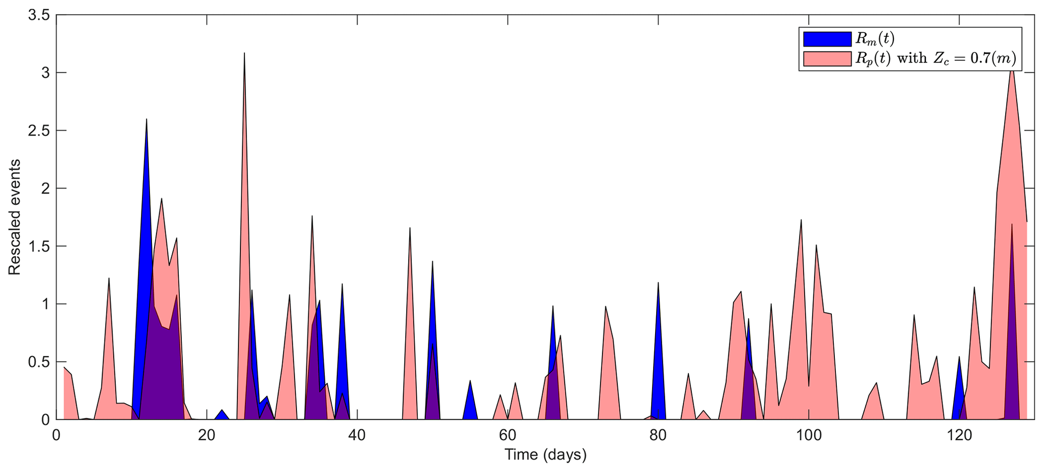
Figure 12Daily time series of the rescaled measured flooded area (Rm) and the rescaled predicted water elevation (Rp) above a beach elevation, Zc=0.7 m, from 23 November 2017 to 31 March 2018 (see definition in Sect. 4.2, Eq. 2). At the selected elevation (Zc=0.7 m), the predicted flooding frequency from water elevation data equals the measured one from flooded area (see Fig. 11); however, the duration of the predicted flooding events is much longer.
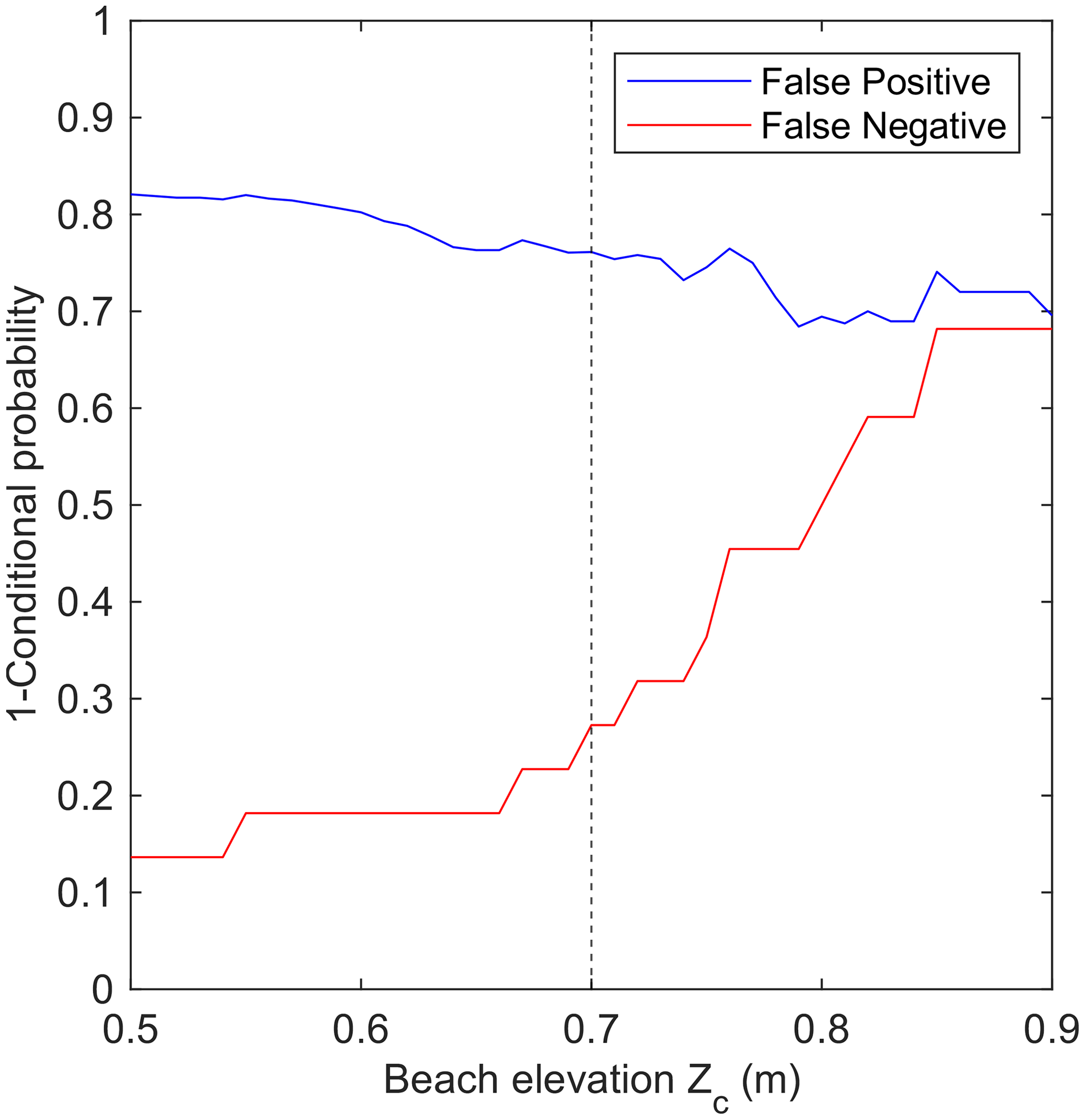
Figure 13Performance of the model predictions when compared to measurements for different beach elevations (Zc). False-positive and false-negative rates are defined in terms of conditional probabilities as the probability of flooding conditions being predicted but not measured and the probability of flooding conditions being measured but not predicted, respectively (see Sect. 4.2 for a detailed definition).
In spite of the numerous uncertainties in the estimation of the actual total water level from offshore wave data, the time series given by Eq. (2) were remarkably similar for the characteristic beach elevation Zc=0.7 m at which the predicted flooding frequency equals the measured one (Fig. 12). Indeed, most measured events were accurately captured by the prediction, including their relative intensity.
We evaluated the performance of the run-up model in predicting the measurements at the daily scale using the conditional probabilities P(m|p) and P(p|m), where P(m|p) is the probability of observing or measuring flooding (m) during a day when flooding conditions were predicted (p) and P(p|m) is the probability of predicting flooding conditions during a day when flooding was observed or measured. Figure 13 shows the rates of false positives , when flooding was predicted but not measured, and false negatives , when flooding was measured but not predicted, for the time series given by Eq. (2) as function of the characteristic beach elevation Zc in the model prediction.
As is already apparent in Fig. 12, at Zc=0.7 m the rate of false negatives is relatively low (∼25%), whereas the rate of false positives is quite high (∼75 %). Since the predicted and measured frequency of flooding events are equal, the large rate of false positives implies the duration of the predicted flooding events is much longer that the observed ones. As the beach elevation increased, the rate of false negatives drastically increased, which supports our indirect estimation of the characteristic beach elevation at our site by comparing the predicted and measured flooding frequencies. However, no similar improvement occurred for the rate of false positives, as the run-up model consistently overpredicted the number of flooding days at all beach elevations.
Summarizing our findings, flooding events obtained from the daily time series of water area A|24 h(t) were uncorrelated and their size followed an exponential distribution with average % (Figs. 9 and 10). Therefore, the frequency of a flooding event of at least a size Sc (in percent of water pixels) is given by
where % is the average size and per month is the frequency of all measured flooding events at the daily scale. Note that λ2 % depends on the selected 2 % threshold for the water area fraction (also appearing in the exponent) separating flooding and non-flooding conditions.
Similarly, as was already mentioned in Sect. 1, Rinaldo et al. (2021) found the overtopping (i.e., flooding) frequency of an elevation Z, relative to MSL, can be approximated as follows:
where m is the approximated average size of HWEs (it was found to be mildly site dependent) and λb=1.5 per month is the overtopping frequency at the reference elevation Zr relative to MSL. This elevation was found to roughly correspond to the characteristic beach elevation at a given site and depends on the local tidal amplitude At and average predicted wave runup as follows:
The average wave runup, predicted using the formulation of Stockdon et al. (2006), can in turn be expressed in terms of the deep-water significant wave height Hs and wavelength L0 as follows:
where the overline means average over the time period analyzed, L0 is calculated from the peak wave period Tp using the deep-water dispersion relation , and the factor a(β) is function of the beach slope β and can be written as follows:
with constant βc=0.087 (Rinaldo et al., 2021). Equations (4)–(7) provide a relatively simple and widely applicable probabilistic model of low-intensity and high-frequency flooding events.
Although our Eq. (3) only gives an indirect measure of actual flooded area by using the fraction of water pixels in an image and is only valid for our field site, it does support the validity of Eq. (4) in describing actual flooding using HWEs.
We studied the stochastic properties of flooding events monitored via 5 min time-lapse imagery for more than 160 d and processed the results using CNN-based image segmentation. We found the frequency of flooding events depended strongly on the timescale at which data were analyzed and decreased from about 6 events per month at the hourly timescale to a plateau of 2.5 events per month at the daily timescale. Furthermore, the correlation between consecutive events also depended on the timescale. Following our statistical analysis of event inter-arrivals, flooding events seem to be correlated for timescales smaller than 10 h, while events are random and independent at larger timescales, thereby following a Poisson process. This change in temporal correlation for timescales around 10 h could be related to the tidal period (which is about 12 h at this location) and the day–night cycle potentially disrupting any local weather pattern behind the flooding event.
We found the size of flooding events was exponentially distributed with average sizes of about 4 % of the camera field of view when data was analyzed at the hourly timescale to a maximum 8 % at the daily or larger timescale. When estimated at the highest 5 min resolution, we also found the actual duration of flooding events typically varies between 10 and 100 min and seemed to follow a power law distribution. The lack of events longer than 3 h in our nearly 6-month period, during which there were no large storms, seems to suggest a physical upper limit for sustained flooding conditions perhaps related to high tides. However, in this region astronomical tides are relatively small and water levels are mainly affected by waves, which would again point to wave runup driving the observed flooding, as suggested by the high-water event analysis. Furthermore, we found a poor correlation between the size and the duration of flooding events.
When focused on the daily timescale, we found that flooding events can be modeled as a Poisson process with exponentially distributed sizes, in agreement with recent findings using a run-up model to predict coastal flooding (Rinaldo et al., 2021). The main probabilistic properties of measured and predicted flooding events can thus be described by Eqs. (3) and (4), respectively. One way to understand the similar form of both equations is through the relation between flooded area and water depth at the shoreline. Assuming the beach slope in our field site is relatively constant, then we would expect both to be proportional, in which case the fraction of water pixels would also correlate with water depth at the shoreline. Therefore, our agreement with Rinaldo et al. (2021) suggests that the exponential distribution is robust with respect to potential variations in the local beach slope during the measurement period and alongshore variations in the flooded area at the spatial scale defined by the camera field of view.
Going beyond the statistical agreement pointed above, the frequency of 1.5 events per month predicted by HWEs (Rinaldo et al., 2021) for natural beaches, albeit lower than the 2.5 events per month measured, was within the confidence bounds of our data, which were relatively large due to the short time period analyzed. Nevertheless, a higher measured flooding frequency was expected because of beach erosion induced by Hurricane Harvey, which would improve the agreement with the model. When focusing on the daily correlation of predicted and measured flooding, the predictions from the analysis of HWEs (Rinaldo et al., 2021) captured most of the occurrence of daily flooding, although it noticeably overpredicts them. The large fraction of false positives in the predicted flooded days (particularly at the end of the measurement period), even after correcting for a different beach elevation, could result from the assumption of a constant beach slope along the whole beach section covered by the camera and for the whole observation period. Since run-up predictions using offshore data (Stockdon et al., 2006, 2014) are essentially valid for a single transect and thus neglect the alongshore variability of the bathymetry or the details of wave shoaling (García‐Medina et al., 2017; Atkinson et al., 2017), it would be difficult to capture the complexity of the site-to-site variability of flooding over a relatively large beach section. On the other hand, it could be that the predicted flooding was taking place somewhere else along the beach and was not captured by our local observations. A final possibility is that our sampling frequency of one picture every 5 min is not high enough to capture all possible large runup events (as predicted by the HWEs formulation), in which case the false positive rate could be lower. This is supported by the fact that the distribution function of the duration of flooding events has a lower limit of 3 min.
Regardless of these sources of potential errors, and more in line with the statistical nature of wave runup data and the uncertainty in the calibration of the model parameters in the first place (García‐Medina et al., 2017; Atkinson et al., 2017), one can argue that the prediction only indicates conditions favorable to flooding events somewhere along the shoreline and not necessarily the actual occurrence of a flooding event at a precise location. This statistical interpretation would agree with our findings.
In addition to our findings characterizing the probabilistic structure, including frequency, intensity and duration, of coastal flooding at our field site, by validating the predictions of Rinaldo et al. (2021), our work also demonstrates the suitability of HWE predictions, based on relatively simple run-up models, for estimating the frequency and intensity of events leading to coastal flooding and dune erosion. Our results thus formalize, i.e., validate and expand, the first probabilistic model of high-frequency low-intensity coastal flooding events driven by wave run-up (e.g., Eqs. 4–7). After further calibration of the model parameters for different locations, this probabilistic model can be very useful in coastal risk management and landscape evolution models.
All data used or generated in this study are available from the Texas Data Repository (TDR) at https://doi.org/10.18738/T8/CDBYNN (Kang, 2023).
ODV designed the study. ODV, RAF and TH installed the field equipment and carried out the observations. BK performed the time series analysis. BK and ODV performed the probabilistic analysis. BK and ODV prepared the manuscript with contributions from all co-authors.
At least one of the (co-)authors is a member of the editorial board of Earth Surface Dynamics. The peer-review process was guided by an independent editor, and the authors also have no other competing interests to declare.
Publisher's note: Copernicus Publications remains neutral with regard to jurisdictional claims made in the text, published maps, institutional affiliations, or any other geographical representation in this paper. While Copernicus Publications makes every effort to include appropriate place names, the final responsibility lies with the authors.
Orencio Durán Vinent and Byungho Kang were supported by the Texas A&M Engineering Experiment Station.
This paper was edited by Sagy Cohen and reviewed by two anonymous referees.
Atkinson, A. L., Power, H. E., Moura, T., Hammond, T., Callaghan, D. P., and Baldock, T. E.: Assessment of runup predictions by empirical models on non-truncated beaches on the south-east Australian coast, Coast. Eng., 119, 15–31, https://doi.org/10.1016/j.coastaleng.2016.10.001, 2017. a, b
Bevacqua, E., Maraun, D., Vousdoukas, M. I., Voukouvalas, E., Vrac, M., Mentaschi, L., and Widmann, M.: Higher probability of compound flooding from precipitation and storm surge in Europe under anthropogenic climate change, Sci. Adv., 5, eaaw5531, https://doi.org/10.1126/sciadv.aaw5531, 2019. a
Cramér, H.: On the composition of elementary errors, Scandinav. Actuar. J., 1928, 13–74, https://doi.org/10.1080/03461238.1928.10416862, 1928. a
Durán Vinent, O., Schaffer, B. E., and Rodriguez-Iturbe, I.: Stochastic dynamics of barrier island elevation, P. Natl. Acad. Sci. USA, 118, e2013349118, https://doi.org/10.1073/pnas.2013349118, 2021. a
García‐Medina, G., Özkan‐Haller, H. T., Holman, R. A., and Ruggiero, P.: Large runup controls on a gently sloping dissipative beach, J. Geophys. Res.-Oceans, 122, 5998–6010, https://doi.org/10.1002/2017jc012862, 2017. a, b
Kang, B.: Time Series Data and Preprocessing Code for Coastal Flooding Probabilistic Analysis, Texas Data Repository [code and data set], https://doi.org/10.18738/T8/CDBYNN, 2023. a
Kang, B., Feagin, R. A., Huff, T., and Durán Vinent, O.: Stochastic properties of coastal flooding events – Part 1: convolutional-neural-network-based semantic segmentation for water detection, Earth Surf. Dynam., 12, 1–10, https://doi.org/10.5194/esurf-12-1-2024, 2024. a, b, c
Lilliefors, H. W.: On the Kolmogorov–Smirnov Test for the Exponential Distribution with Mean Unknown, J. Ame. Stat. Assoc., 64, 387–389, https://doi.org/10.2307/2283748, 1969. a
Moftakhari, H. R., AghaKouchak, A., Sanders, B. F., and Matthew, R. A.: Cumulative hazard: The case of nuisance flooding, Earth's Future, 5, 214–223, https://doi.org/10.1002/2016EF000494, 2017. a, b
Moftakhari, H. R., AghaKouchak, A., Sanders, B. F., Allaire, M., and Matthew, R. A.: What Is Nuisance Flooding? Defining and Monitoring an Emerging Challenge, Water Resour. Res., 54, 4218–4227, https://doi.org/10.1029/2018WR022828, 2018. a, b
Muis, S., Verlaan, M., Winsemius, H. C., Aerts, J. C. J. H., and Ward, P. J.: A global reanalysis of storm surges and extreme sea levels, Nat. Commun., 7, 11969, https://doi.org/10.1038/ncomms11969, 2016. a
Rinaldo, T., Ramakrishnan, K. A., Rodriguez-Iturbe, I., and Durán Vinent, O.: Probabilistic structure of events controlling the after-storm recovery of coastal dunes, P. Natl. Acad. Sci. USA, 118, e2013254118, https://doi.org/10.1073/pnas.2013254118, 2021. a, b, c, d, e, f, g, h, i, j, k, l, m, n, o, p, q, r, s, t, u, v, w, x, y, z
Serafin, K. A. and Ruggiero, P.: Simulating extreme total water levels using a time-dependent, extreme value approach, J. Geophys. Res.-Oceans, 119, 6305–6329, https://doi.org/10.1002/2014jc010093, 2014. a
Serafin, K. A., Ruggiero, P., and Stockdon, H. F.: The relative contribution of waves, tides, and nontidal residuals to extreme total water levels on U.S. West Coast sandy beaches, Geophys. Res. Lett., 44, 1839–1847, https://doi.org/10.1002/2016GL071020, 2017. a
Stockdon, H. F., Holman, R. A., Howd, P. A., and Sallenger, A. H.: Empirical parameterization of setup, swash, and runup, Coast. Eng., 53, 573–588, https://doi.org/10.1016/j.coastaleng.2005.12.005, 2006. a, b, c, d, e
Stockdon, H. F., Thompson, D. M., Plant, N. G., and Long, J. W.: Evaluation of wave runup predictions from numerical and parametric models, Coast. Eng., 92, 1–11, https://doi.org/10.1016/j.coastaleng.2014.06.004, 2014. a, b, c
Sweet, W., Park, J., Marra, J., Zervas, C., and Gill, S.: Sea Level Rise and Nuisance Flood Frequency Changes around the United States, NOAA technical report NOS CO-OPS 073, NOAA, https://repository.library.noaa.gov/view/noaa/30823 (last access: 5 December 2023), 2014. a
Ward, P. J., Couasnon, A., Eilander, D., Haigh, I. D., Hendry, A., Muis, S., Veldkamp, T. I. E., Winsemius, H. C., and Wahl, T.: Dependence between high sea-level and high river discharge increases flood hazard in global deltas and estuaries, Environ. Res. Lett., 13, 084012, https://doi.org/10.1088/1748-9326/aad400, 2018. a
- Abstract
- Introduction
- Defining and measuring flooding events
- Statistical analysis of measured flooding events
- Comparison with run-up model predictions
- Towards a probabilistic model of low-intensity and high-frequency flooding events
- Discussion and conclusion
- Data availability
- Author contributions
- Competing interests
- Disclaimer
- Acknowledgements
- Review statement
- References