A numerical model for duricrust formation by laterisation

Duricrusts form near the top of or within the regolith. Once exhumed, they are resistant to erosion and are often observed capping hilltops. Two hypotheses have been proposed to explain their formation. One calls upon seasonal fluctuations in water table height causing cycles of dissolution and precipitation that concentrate hardening species transported from distant sources. The other assumes that hardening is the ultimate phase of laterisation of the regolith by progressive leaching of the soluble elements that leads to in situ concentration of the hardening species. Here we propose a numerical model for the formation of duricrusts following the latter hypothesis, which we will term the in situ or laterisation (LAT) model. In Fenske et al. (2025), we developed a similar model representing the other model (named here the transport or Water Table Fluctuation (WTF) model).

The LAT model we present here assumes that the rate of hardening is a self-limiting process that takes place at a rate determined by a laterisation time scale, τ_l, and is linearly proportional to precipitation rate. Laterisation is accompanied by mass loss, at a rate set by a mass loss time scale, τ_m, that can potentially be different from τ_l and causes lowering of the topographic surface. We also test three laterisation modes, that depend on whether laterisation takes place above the water table only (percolation mode), below the water table (saturated mode) or everywhere (everywhere mode). This model for the formation of duricrusts is embedded in a previously published model for regolith formation (Braun et al., 2016).

Here we present results obtained from the new LAT model by varying both the model parameters and the external forcing functions, namely, U the uplift rate and P, the precipitation rate. We show that duricrust formation by laterisation is favored by a small uplift rate as well as a strong precipitation rate. The smaller the laterisation time scale and the mass loss time scale, the thicker the duricrust, but if the ratio between the two time scales, τ_m $/$ τ_l is too small, no duricrust can form or, in the saturated mode, the duricrust is progressively buried during its formation. We also derive a simple analytical expression for the conditions under which a duricrust will form within a regolith. This relationship implies that, as shown in Braun et al. (2016), for regolith to form, the time scale for primary weathering, τ_w, that controls the rate of propagation of the weathering front into the bedrock must be smaller than the erosion time scale, τ_e, that controls the rate of surface erosion, and for a duricrust to form, the time scale for secondary weathering, or laterisation time scale, τ_l, must be smaller than the primary weathering time scale.

The model also predicts hardening (or duricrust) age distributions that can be compared to ages obtained by (U-Th) $/$ He dating of goethite in ferricretes for example. We show that these age distributions can be used to differentiate between the different modes of laterisation. We also show how peaks in age distributions appear to correlate very well with climatic events, but not with periods of enhanced uplift (or base level fall). The model also predicts the total mass loss by chemical vs. physical erosion. We show that the ratio between the two is mostly a function of the laterisation time scale and how it varies during climate or tectonic cycles.

Finally, we show how the model predictions can be compared to those of the WTF model to help determine by which process a given duricrust formed. We also show, however, that there might be situations where the geometry, thickness and position of the duricrusts may not be unequivocal signatures of a given process.

1 Introduction

Regolith covers most of the surface of telluric planets. On Earth, it is defined as the layer at the interface between the solid Earth, hydrosphere and biosphere (Taylor and Eggleton, 2001). For decades, the regolith has been the subject of many studies in a variety of environments, but many aspects of its formation and evolution remain unclear, particularly within cratonic areas. Cratons are geologically stable regions, that often exhibit geomorphic features that may suggest otherwise. Among these features are duricrusts. Duricrusts are hard mineral layers, which are commonly observed capping hills (Azmon and Kedar, 1985; Twidale and Bourne, 1998; Taylor and Eggleton, 2001) but also along valley bottoms (Radtke and Brückner, 1991; Chudasama et al., 2018). In many instances, they appear to protect landscapes (e.g. Tardy, 1993; Taylor and Eggleton, 2001; Chardon, 2023; Fenske et al., 2025), but they can also lead to the formation of inverted topographies (Goudie, 1985; Twidale and Bourne, 1998; Taylor and Eggleton, 2001, 2017).

Different types of duricrusts exist, namely calcretes (made of calcium carbonates), silcretes (silica rich duricrusts) (Goudie, 1985; Nash et al., 1994), ferricretes (iron oxide and oxide-hydroxide rich) (Bourman, 1985; Goudie, 1985; Tardy, 1993), alcretes, or bauxitic crusts, which are rich in aluminum (Goudie, 1985; Taylor and Eggleton, 2001; Horbe and Anand, 2011; dos Santos Albuquerque et al., 2020) or even gypcretes (gypsum rich duricrusts) (Dixon and McLaren, 2009).

Due to their characteristics and complex formation conditions, duricrusts are used as paleo-climatic, tectonic and geochronological markers around the world (e.g. Goudie, 1985; Tardy, 1993; Twidale and Bourne, 1998; Alonso-Zarza, 2003) while also being useful mineral sources (e.g. Bustillo et al., 2013; Chudasama et al., 2019). As such, understanding their formation, evolution, and characteristics is crucial.

1.1 A typical pedogenic duricrust forming regolith profile

A typical simplified duricrust forming profile (Fig. 1), from bottom to top, can be defined as follows: (1) the bedrock, (2) the saprolite, (3) the mottled zone and (4), in some cases, the duricrust.

• The bedrock: at the base of the profile, it is separated from the overlying regolith by a weathering front that propagates downwards by primary weathering.

• The saprolite: it begins at the weathering front. The saprolite is the thickest and softest part of the profile and can be subdivided into coarse saprolite in the lower part of the profile, where the bedrock structure can still be observed, and fine saprolite in the upper part of the profile, where no structure is left. It is a clay-rich material.

• The mottled zone: it is defined by white and colorful patches due to elemental segregation of minerals. Depending on the profile type, the colorful nodules are either aluminium, iron, silica or carbon rich, while the white patches are usually clays, for example kaolinite.

• The duricrust: it is a hard mineral crust at the top of the profile that can usually be subdivided into a massive duricrust below and a granular or pisolithic duricrust on top.

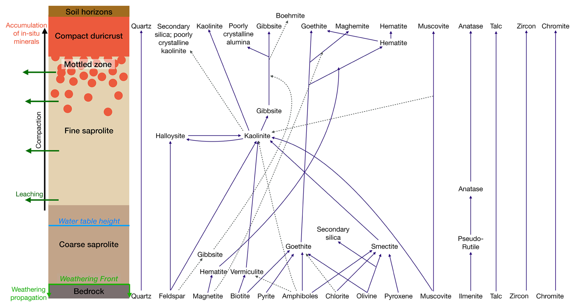
Figure 1 On the left, simplified weathering profile with duricrust formation. On the right, chemical reaction pathways typical during laterisation, leading to the formation of secondary minerals, and ultimately to the formation of iron and/or aluminium rich duricrusts. Modified according to Anand (2005).

The profile layers result from weathering evolution. Each layer grows at the expense of the layer below (Tardy, 1993). With increasing weathering at the top, the most soluble minerals will be dissolved and transported, i.e., leached out of the system, while the less soluble minerals will accumulate. This exchange is most noticeable in the mottled zone, where accumulated minerals cement into growing nodules, while the white pockets are leached, creating a highly porous environment (Tardy, 1992, 1993; Alonso-Zarza and Wright, 2010).

1.2 Duricrust formation: mechanisms and theoretical divergences

Duricrust formation has been thoroughly investigated during the last century (e.g. Paton and Williams, 1972; Netterberg, 1978; Butt, 1985; Watson, 1988; Nahon, 1991; Milnes, 1992; Tardy, 1993; Nash et al., 1994; Webb and Golding, 1998; Twidale and Bourne, 1998; Nash and Shaw, 1998; Alonso-Zarza and Wright, 2010; Nash, 2011; Taylor and Eggleton, 2017; Thiry and Milnes, 2017; Heller et al., 2022; Rozefelds et al., 2024). While the precise conditions that lead to the formation of duricrusts remain the subject of research, two important aspects have been identified. Firstly, different types of duricrusts tend to form under different climatic conditions, from hyper-arid, e.g. gypcretes (Dixon and van Blanckenburg, 2012) to humid, e.g bauxites (Tardy, 1993). Secondly, duricrust formation generally occurs over a time frame extending from tens of thousands to millions of years. A compilation of formation rates is available in Fenske et al. (2025). The time needed to form a crust mostly depends on the duricrust type. For instance, calcretes generally form faster than ferricretes and silcretes (Fenske et al., 2025). The formation time scale is however also dependent on the duricrust formation processes (Alonso-Zarza, 2003).

The assumed formation processes for duricrusts commonly fall into two main categories (Goudie, 1985; Bourman, 1985, 1996): (1) formation by absolute accumulation, adding material to the regolith, also called the transport model, lateral model (Bourman, 1985; Bourman et al., 2020) or hydrological model (Fenske et al., 2025) and (2) formation by relative accumulation, removing material from the regolith (Goudie, 1985; Bourman, 1985), called the in situ model, residue model (Bourman, 1985; Bourman et al., 2020) or laterisation model (Tardy, 1993). Finally, another duricrust formation mechanism exists that involves the erosion of preexisting duricrusts and their subsequent reworking at lower elevations (Twidale and Bourne, 1998; Taylor and Eggleton, 2001).

Defining system characteristics and boundaries is important, as depending on the observation scale the accumulation in one system can be either absolute (i.e., where the regolith column is enriched by external sources) or relative (i.e., where the regolith column is solely enriched by the underlying bedrock) (McFarlane, 1984; Goudie, 1985; Tardy, 1993). Goudie (1985) also highlighted that some profiles evolve exclusively through absolute accumulation, e.g. by river or groundwater transport, or by relative accumulation, e.g. by laterisation processes. However, both processes can be found at the same scale in the same system (Goudie, 1985). For example recently, Monsels and van Bergen (2017) observed the formation of bauxites in Suriname, which held evidence of both in situ and transport processes.

1.3 Transport based or hydrological hypothesis

According to this hypothesis, duricrusts form at the water table height under a climate with alternating wet and dry periods. During the wet season, a high water table transports minerals like iron or calcite to topographic lows (Fig. 2a). During the dry season, the water table drops, and minerals precipitate due to changing redox and pH conditions. Precipitation occurs in aerobic environments near the water table, while deeper zones remain anaerobic and do not form duricrusts. This process is repeated during tens of thousands of years, during which minerals accumulate by forming nodules and ultimately, a duricrust. Duricrusts generally form several metres below the surface, except in valleys where the water table is close to the surface and duricrusts can form directly at the surface. Transport-based duricrusts thus register the paleo-height of the water table.

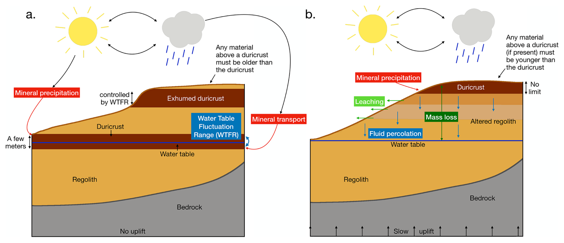
Figure 2 (a) Example of a hill under WTF model conditions. An old exhumed duricrust is observed at the top of the hill while a new duricrust is formed at the water table height. The processes and environment conditions leading to duricrust formation are depicted by arrows. (b) Example of a hill under LAT percolation model conditions. The duricrust forms at the top of the hill, while hardening influences the shape of the hill and the regolith below the duricrust. Arrows highlight the processes and necessary conditions to duricrust formation.

In the hydrological hypothesis, mineral accumulation that leads to duricrust formation is absolute (Goudie, 1985), and there is no genetic link between the duricrust and the layers below (Ollier and Galloway, 1990). Most types of duricrusts may form according to the hydrological hypothesis, but it is thought to apply mostly to silcretes (Ritter et al., 2023), calcretes (Goudie, 1985), and ferricretes (Ollier and Galloway, 1990; Bourman, 1993). Evidence of alcretes partially forming in this way have also been observed (Monsels and Bergen, 2019)

Stability of the system is essential for the formation of a duricrust. If a base level change affects the region or the climate changes, duricrusts can be exhumed to the surface, where they are more resistant to erosion than neighboring geological layers. This can lead to duricrusts either capping hill-tops (Taylor and Eggleton, 2001; Alonso-Zarza, 2003) or to landscape inversion of whole drainage systems (Nash et al., 1994; Twidale and Bourne, 1998; Taylor and Eggleton, 2001).

In Fenske et al. (2025), we developed a numerical model that simulates duricrust formation by water table fluctuations. Here, we will refer to it as the WTF model. We direct the reader to Fenske et al. (2025) for a complete description of the model and of its behavior.

1.4 In-situ, residue or laterisation hypothesis

In this case, duricrusts are considered the ultimate compacting stage of laterisation, bauxitisation and weathering processes leading to what are called pedogenic duricrusts (Grant and Aitchison, 1970; Paquet and Clauer, 1997), that include mostly alcretes and ferricretes (Tardy and Roquin, 1992), although pedogenic calcretes (Alonso-Zarza and Wright, 2010) or silcretes (Taylor and Eggleton, 2017; Thiry and Milnes, 2017) have also been described.

According to this process, mineral accumulation is relative (Goudie, 1985), where the regolith column is enriched solely by the underlying bedrock and material present in the system (Fig. 2b). There is a genetic link between the duricrust and the underlying bedrock and regolith (Tardy and Roquin, 1992). Through secondary weathering processes from the weathering front to the surface, the more soluble minerals dissolve and are carried away, or leached, from the system, while less soluble minerals remain and accumulate (Fig. 1). Over time, gravity causes the porous material to compact, leading to the cementation and hardening of a duricrust (e.g. Tardy, 1992, 1993; Taylor and Eggleton, 2001; Tardy and Roquin, 1998; Nahon and Bocquier, 1983; Nahon, 1991; Alonso-Zarza and Wright, 2010; Thiry and Milnes, 2017).

1.5 Laterisation and the water table

In a weathering profile, two weathering stages are observed. The first stage occurs at the weathering front, where primary weathering processes dissolve and re-precipitate bedrock minerals to transform the bedrock into the more permeable regolith. The second stage involves secondary weathering, which alters the neo-formed minerals within the regolith column (Anand and Paine, 2002; Anand, 2005). This process can lead to laterisation (formation of a laterite) and the formation of hardened material, such as a duricrust. The efficiency of secondary weathering is linked to fluid transport processes, which has been hypothesized to fall into three modes. In the first mode, secondary weathering occurs under non-saturated conditions above the water table. It is primarily driven by vertical water movements, such as percolation from the surface or capillary rise from the water table (Tardy, 1993; Vasconcelos and Conroy, 2003; Bonsor et al., 2014; Fritsch et al., 2011; Girard et al., 2002; Monteiro et al., 2014, 2018; Riffel et al., 2016; Spier et al., 2006, 2019). In this case, a duricrust would form at or near the surface. The second mode involves secondary weathering under more saturated conditions within the groundwater, driven by lateral groundwater flow (Trendall, 1962; Riffel et al., 2015; Chardon et al., 2018). In this second case, duricrusts form within the regolith. In the third mode, secondary weathering affects the entire regolith column, where both percolation and groundwater movements exert equal influence (Tardy and Nahon, 1985; Tardy, 1993; Braun et al., 2005, 2012; Fritsch et al., 2011). One could argue that the mode that is preferred in a given environment may depend on the permeability, itself related to fracturation and porosity, of the bedrock and, consequently, the regolith. It is thus potentially more likely that the second mode be active when the regolith forms on top of a sedimentary unit or a highly fractured bedrock. However, many authors appear to support the percolation hypothesis, with one of the main arguments being that the resulting duricrusts form at the surface or near the surface (Stephens, 1970; Firman, 1993; Taylor and Eggleton, 2001). However, duricrust formation in the subsurface is also observed for pedogenic duricrusts (Firman, 1993; Fujioka et al., 2005). To test the validity of these modes, we implemented all three into the model.

2 Modelling weathering and duricrust formation

Previous work by e.g. Lebedeva et al. (2007), Ferrier and Kirchner (2008), Brantley and White (2009), Maher (2010), Lebedeva et al. (2010), Pelletier (2010), Lebedeva and Brantley (2013), Norton et al. (2014), Pelletier et al. (2016), Braun et al. (2016), Brantley et al. (2017), Lebedeva and Brantley (2018) has led to the development of models for the formation of the regolith that were either based on physical or chemical processes. Examples where the process of duricrust formation was envisaged are less numerous. Soler and Lasaga (1996) proposed a 1D geochemical model for bauxite formation and Lichtner and Biino (1992) suggested a model for iron evolution in copper and ferrous crusts, but they did not envisage the consequences of the duricrust formation and exhumation on erosional processes. Conversely, Sacek et al. (2019) developed a highly simplified model for duricrust formation at the continental scale that they used to study the consequences of duricrust formation on the patterns and timing of surface erosion. Fenske et al. (2025) developed a model for duricrust formation through the transport hypothesis, i.e., by water table fluctuation (Fenske, 2025). Although highly simplified too, this model assumed that duricrust formation is solely due to water table movements during seasonal cycles, with transport and precipitation of minerals towards topographic lows. Using the model Fenske et al. (2025) demonstrated that alternating periods of tectonic quiescence and uplift were necessary to form the duricrust and expose it to the surface. They also showed that exposed duricrusts protect surface features but over a time scale that is much reduced in comparison to their assumed intrinsic strength (resistance to erosion).

In the following we propose to present a second model for duricrust formation that is based on the second most commonly assumed hypothesis that duricrusts are the ultimate compaction product of laterisation, that result from the removal of the most soluble minerals, accumulation of least soluble minerals and associated volume and mass loss.

2.1 Regolith formation model

As we did in Fenske et al. (2025), we base the new duricrust model (Fenske, 2025) on the regolith formation model developed by Braun et al. (2016). This model is designed to represent processes that evolve on geological time scales and at the scale of a single hill (Fig. 3), although its predictions can be generalised to any topographic feature affected by weathering in which the water table is connected to a well-defined and unique base level. The model predicts the surface geometry, the propagation of the weathering front and the geometry of the water table (Braun et al., 2016). It is composed of three components representing three different physical processes. The first is a surface process component, where it is assumed that topography is affected by tectonic uplift and sediment transport, defined by:

$$\begin{array}{}\text{(1)}& {\displaystyle \frac{\partial z}{\partial t}}=U+{\displaystyle \frac{\partial }{\partial x}}{K}_D{\displaystyle \frac{\partial z}{\partial x}},\end{array}$$

where z is the topographic height (m), U the uplift rate (m yr⁻¹), K_D the surface transport coefficient, which varies between 0 and 1, x the space- and t the time coordinates. The second is a weathering component which describes weathering front propagation as proportional to fluid velocity, defined by:

$$\begin{array}{}\text{(2)}& {\displaystyle \frac{\partial B}{\partial t}}=FK{\displaystyle \frac{\partial H}{\partial x}}-{\displaystyle \frac{\partial z}{\partial t}},\end{array}$$

where B is the weathering profile thickness (in m), F the ratio between weathering front velocity and fluid velocity (dimensionless), K the hydraulic conductivity (in m yr⁻¹) and H, the height of the water table (in m). The third is a hydrological component, which assumes that flow is essentially lateral and velocity proportional to the slope of the water table, leading to the following equation:

$$\begin{array}{}\text{(3)}& K\left(H-z+B\right){\displaystyle \frac{\partial H}{\partial x}}+\underset{L}{\overset{x}{\int }}P\mathrm{d}{x}^{\prime }=\mathrm{0},\end{array}$$

where L is the length of the hill (in m), and P is the precipitation rate (in m yr⁻¹).

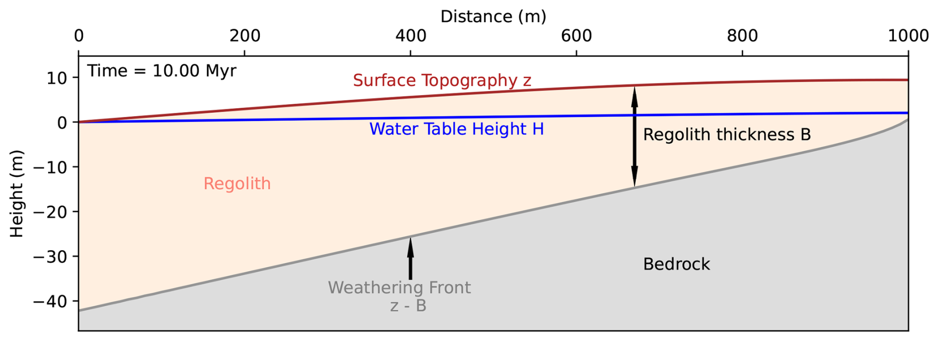
Figure 3 The problem setup, including the defined quantities and variables, follows the framework outlined by Braun et al. (2016). The figure shows a steady-state scenario resulting from solving the differential equations described in the text. It depicts the weathering front (in dark grey), the water table geometry (in blue), and the topography (in brick red), after 10 Myrs of model evolution (Fenske et al., 2025).

Two dimensionless numbers Ω and Γ, control the rate of regolith formation and its geometry at steady-state (Braun et al., 2016) as shown in Fig. 4. These are defined by:

$$\begin{array}{}\text{(4)}& \mathrm{\Omega }={\displaystyle \frac{FKL}{\mathrm{2}{K}_D}}={\displaystyle \frac{FK\stackrel{\mathrm{‾}}{S}}{U}}\text{and}\mathrm{\Gamma }={\displaystyle \frac{K{\stackrel{\mathrm{‾}}{S}}^{\mathrm{2}}}{P}},\end{array}$$

where $\stackrel{\mathrm{‾}}{S}$ is the mean surface slope. Ω defines if and where a regolith can form in the landscape, and its thickness. If Ω is greater than 0.5, a weathering profile will develop at the top of the hill and if Ω is greater than 1 then a regolith will cover the whole hill. Γ describes regolith geometry. The regolith can be either thickest at the top of a hill, when $\frac{{\mathrm{\Omega }}^{\mathrm{2}}}{\mathrm{\Omega }-\mathrm{1}}$ < Γ; or at its base, when $\frac{{\mathrm{\Omega }}^{\mathrm{2}}}{\mathrm{\Omega }-\mathrm{1}}$ > Γ. Three cases are shown in Fig. 4 to illustrate this behavior. In the first and second cases (panels a and b), ${\mathrm{\Omega }}^{\mathrm{2}}/(\mathrm{\Omega }-\mathrm{1})$ ≈ Γ and the regolith has uniform thickness. In the third case (panel c), ${\mathrm{\Omega }}^{\mathrm{2}}/(\mathrm{\Omega }-\mathrm{1})$ < Γ and the regolith is thickest at the top of the hill. These variations in geometry have been obtained by varying F that controls the rate of weathering front advance per unit fluid velocity (mostly controlled by the bedrock composition) and K, the regolith hydraulic conductivity controlling the slope of the water table per unit surface infiltration. Similar results could have been obtained by varying the precipitation rate, P or the uplift rate U, as shown in Braun et al. (2016).

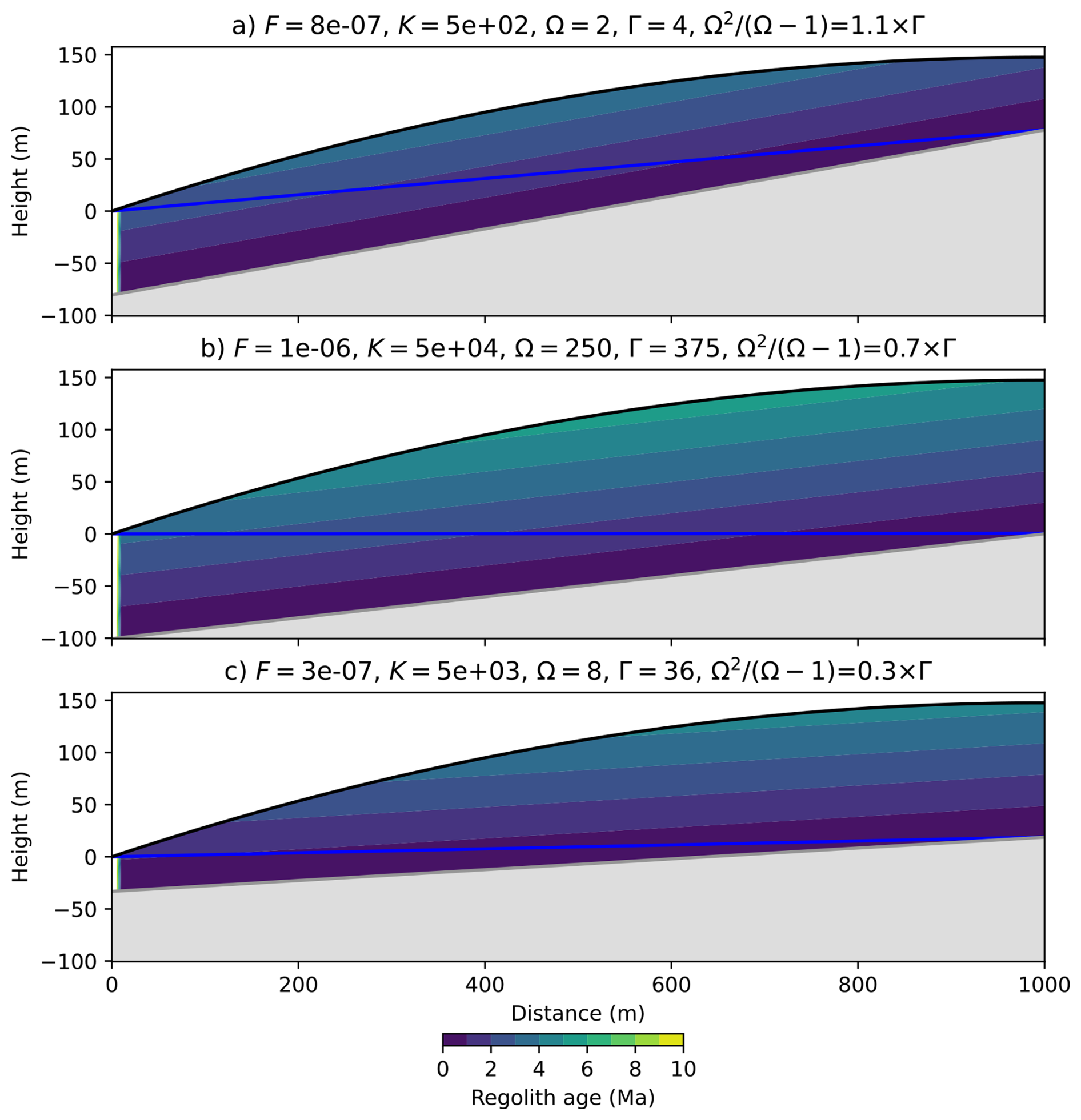
Figure 4 Steady-state solutions of three regolith model run experiments in which K and F were varied to produce distinct regolith geometries. The blue line represents the geometry of the water table. The grey shaded area corresponds to the intact bedrock. In the regolith, i.e., between the surface and the weathering front, the color contours correspond to the predicted age of the regolith, i.e., the time since a rock particle crossed the weathering front.

All three geometries shown in Fig. 4 are typical of anorogenic areas, leading to thick regolith layers of up to 100 m. For the remainder of this manuscript, we will use model parameters K and F that correspond to panel (b), with a regolith thickness of 100 m at the base level and 150 m at the top of the hill.

Braun et al. (2016)'s regolith model assumes homogeneous properties in the regolith layer, which does not allow to track weathering changes and the formation of duricrusts. In Fenske et al. (2025), we have modified the weathering model of Braun et al. (2016) by adding a component that represents the formation of duricrusts following the transport or hydrological hypothesis. For this, we added a new equation governing the evolution of a hardening coefficient κ, that depends on an assumed water table fluctuation range, λ, and a formation time scale, τ, for which we derived constraints from the literature (Fenske et al., 2025).

Building on this, we introduce now an alternative hardening equation to predict (1) the distribution of hardening, (2) duricrust formation through laterisation, (3) the conditions under which pedogenic duricrusts form, (4) as well as the potential geomorphic feedback when the duricrusts are exposed to the surface. In this way, both the transport and the in situ hypotheses have a numerical implementation, enabling us to compare the predictions of the two opposing models of duricrust formation and, possibly, to differentiate in which environmental conditions they each prevail.

2.2 New proposed model: the in situ hypothesis

In this article, we present a new component that we have incorporated to the weathering model that represents the formation of duricrusts according to the in situ hypothesis. Similarly to the transport model developed in Fenske et al. (2025), we propose to use a simple parametric representation of the process based on as few parameters as possible, which we will constrain by comparing the model predictions to observations.

In the model, we will assume that the entire regolith above the weathering front can be subjected to laterisation, which will lead to hardening and mass loss, and ultimately duricrust formation. Different degrees of hardening/mass loss could be regarded as corresponding to the different layers forming the regolith column (saprolite, mottled layer, mineralization zone, and duricrust). Here we will limit this comparison by differentiating between the duricrust and the rest of the regolith layer by introducing a threshold hardening value, as done in Fenske et al. (2025). For simplicity, we will assume that the hardening only affects the resistance to surface erosion, not the hydraulic conductivity. Also we will consider three possibilities: (1) that laterisation takes places above the water table only, (2) below the water table only or (3) everywhere in the regolith layer. Our model will not include the effect of biological activity, which is known to affect the rate of laterisation and duricrust formation (Goudie, 1985; Monteiro et al., 2014), but will include a dependence on precipitation.

For simplicity and ease of comparison with the water table fluctuation (WTF) model, we will refer to the in situ model as the “laterisation model” or “LAT model”, although we acknowledge that laterisation typically applies to the formation of alcretes or ferricretes and not to e.g. calcretes or silcretes.

3 Methods

3.1 Hardening and duricrust formation

As we did in Fenske et al. (2025), we introduce a hardening coefficient κ for the formation of duricrusts through laterisation (LAT) (Fig. 5) to the Braun et al. (2016) model. κ values vary between 0 and 1. The hardening coefficient evolves both in the vertical and horizontal directions, i.e. κ = κ(x,y), within the regolith layer. We will focus on how laterisation influences the hardening coefficient κ and causes mass loss, by adding a differential equation governing the time evolution of the parameter κ:

$$\begin{array}{}\text{(5)}& {\displaystyle \frac{\partial \mathit{\kappa }}{\partial t}}=-{\displaystyle \frac{\mathit{\kappa }}{{\mathit{\tau }}_{\mathrm{l}}}}{\displaystyle \frac{P}{P_{\mathrm{ref}}}}-\left(FK{\displaystyle \frac{\partial H}{\partial x}}-v_{\mathrm{m}}\right){\displaystyle \frac{\partial \mathit{\kappa }}{\partial y}}.\end{array}$$

In this equation, τ_l is the laterisation time scale (in years), P and P_ref (in m yr⁻¹) represent precipitation and reference precipitation respectively, and v_m, the velocity generated by volume reduction associated with mass loss, given by:

$$\begin{array}{}\text{(6)}& v_{\mathrm{m}}=\underset{\mathrm{0}}{\overset{y}{\int }}\dot{C}\mathrm{d}{y}^{\prime },\end{array}$$

where $\dot{C}$ is the rate of mass loss, which we will assume proportional to the material rate of hardening,$\frac{d\mathit{\kappa }}{dt}$, such that:

$$\begin{array}{}\text{(7)}& v_m=\underset{\mathrm{0}}{\overset{y}{\int }}\mathit{\beta }{\displaystyle \frac{d\mathit{\kappa }}{dt}}dy=-{\displaystyle \frac{\mathit{\beta }}{{\mathit{\tau }}_{\mathrm{l}}}}{\displaystyle \frac{P}{P_{\mathrm{ref}}}}\underset{\mathrm{0}}{\overset{y}{\int }}\mathit{\kappa }d{y}^{\prime }\end{array}$$

and, introducing the mass loss time scale, ${\mathit{\tau }}_{\mathrm{m}}={\mathit{\tau }}_{\mathrm{l}}/\mathit{\beta }$, we get:

$$\begin{array}{}\text{(8)}& v_{\mathrm{m}}={\displaystyle \frac{\mathrm{1}}{{\mathit{\tau }}_{\mathrm{m}}}}{\displaystyle \frac{P}{P_{\mathrm{ref}}}}\underset{\mathrm{0}}{\overset{y}{\int }}\mathit{\kappa }\mathrm{d}{y}^{\prime }.\end{array}$$

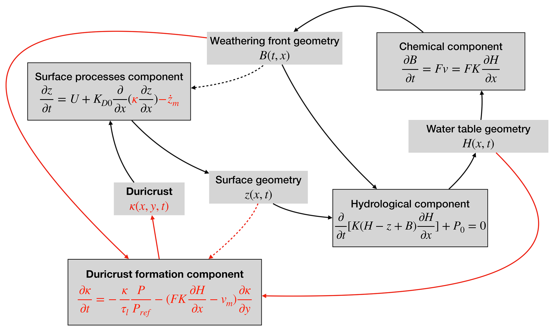
Figure 5 The four interconnecting components in the new LAT model, modified from Braun et al. (2016). The hydrological component, the surface process component and the chemical component are defined by Braun et al. (2016). The new duricrust formation component (in red) is directly connected to the water table geometry H, the weathering front geometry B (concrete arrows), and the hardening coefficient κ directly influences the surface process component. The duricrust formation component is indirectly influenced by surface geometry z (dashed arrows).

Equation (5) is composed of three parts. The first, $\frac{\mathit{\kappa }}{{\mathit{\tau }}_{\mathrm{l}}}\frac{P}{P_{\mathrm{ref}}}$, is a self-limiting term that represents the hardening process taking place at a rate controlled by τ_l but also in proportion to precipitation P. The absolute value of P_ref is arbitrary. What matters is how P varies with respect to this reference value. This is why in the evolution equation for κ precipitation always appears normalized by P_ref. The second, $-FK\frac{\partial H}{\partial x}\frac{\partial \mathit{\kappa }}{\partial y}$ represents advection, proportional to vertical movements of the regolith with respect to the weathering front, thus proportional to the weathering front velocity. The third, $v_{\mathrm{m}}\frac{\partial \mathit{\kappa }}{\partial y}$, represents another vertical velocity due to mass loss, limited by the mass loss time scale τ_m.

Furthermore, to implement the three different secondary weathering hypotheses in the model, we introduce a parameter, C, which enables to set where secondary weathering takes place:

• when C = −1, secondary weathering is limited to the region above the water table through percolation and capillary rise; we call this the “percolation mode”;

• when C = 0, secondary weathering is limited to the region below the water table through groundwater movements; we call this the “saturated mode”;

• when C = 1, secondary weathering takes place in the entire regolith layer through the combined processes; we call this the “everywhere mode”.

As depicted in Fig. 5, the numerical model is composed of four differential equations, each encompassing and connecting different unknowns. The three first equations stem from Braun et al. (2016), while by adding the fourth hardening component, we link the hardening coefficient κ, with the water table height H, the regolith thickness B and the topographic elevation z. In particular, the hardening coefficient κ directly influences the surface component z (Fig. 5), previously defined by Eq. (1) (Braun et al., 2016). However, the surface resistance to erosion evolves through the formation of a duricrust, thus the surface component is redefined by:

$$\begin{array}{}\text{(9)}& {\displaystyle \frac{\partial z}{\partial t}}=U+K_{D\mathrm{0}}{\displaystyle \frac{\partial }{\partial x}}\left(\mathit{\kappa }{\displaystyle \frac{\partial z}{\partial x}}\right)-{\dot{z}}_{\mathrm{m}},\end{array}$$

where K_D0 is diffusivity or reference transport coefficient, and represents a regolith-layer-characteristic transport coefficient without hardening, and ${\dot{z}}_{\mathrm{m}}$ is the surface vertical velocity due to mass loss in the underlying column defined by:

$$\begin{array}{}\text{(10)}& {\dot{z}}_{\mathrm{m}}=-{\displaystyle \frac{\mathrm{1}}{{\mathit{\tau }}_{\mathrm{m}}}}{\displaystyle \frac{P}{P_{\mathrm{ref}}}}\underset{\mathrm{0}}{\overset{B}{\int }}\mathit{\kappa }\mathrm{d}y\end{array}$$

Interestingly, the last two terms on the right-hand side of Eq. (9) represent the mass loss by physical and chemical erosion, respectively. Thus, we can easily compute the flux of material removed from the system by physical erosion, ϕ_P and chemical erosion, ϕ_C by integrating these terms over the entire length of the model:

$$\begin{array}{}\text{(11)}& \begin{array}{rl}& {\mathit{\varphi }}_{\mathrm{P}}=-\underset{\mathrm{0}}{\overset{L}{\int }}{K}_{D\mathrm{0}}{\displaystyle \frac{\partial }{\partial x}}\mathit{\kappa }{\displaystyle \frac{\partial z}{\partial x}}\mathrm{d}x\text{and}\\ & {\mathit{\varphi }}_{\mathrm{C}}=\underset{\mathrm{0}}{\overset{L}{\int }}\left({\displaystyle \frac{\mathrm{1}}{{\mathit{\tau }}_{\mathrm{m}}}}{\displaystyle \frac{P}{P_{\mathrm{ref}}}}\underset{\mathrm{0}}{\overset{B}{\int }}\mathit{\kappa }\mathrm{d}y\right)\mathrm{d}x\end{array}\end{array}$$

As a reminder, three of the four components, B, H and z are solved for in the x direction, while the hardening component is solved in the y direction, making the model partially 2D, as no equation is solved in both the x- and y-spatial directions.

In the same way as in Fenske et al. (2025), the numerical stability and accuracy of the model is assured by the total variation diminishing method (van Leer, 1974). We also combined it with a 1D finite volume method described in Campforts and Govers (2015) in the vertical y direction.

Note that for some model values, for example for low values of the uplift rate U, or low values of the mass loss time scale τ_m, rapid lowering of the surface topography may lead to the formation of a local minimum (i.e., the topography has become negative), which is conflicting with our assumption that the base level is fixed along the left-hand side of the model (i.e., at x = 0). When such a situation arises, we artificially reset the topography between the base level and the local minimum to be equal to that of the local minimum. This mimics the effect of a lowering of the base level or sedimentation of material on top of the profile.

For all numerical scenarios shown in this study, the resolution of the model is set to Δx = 10 m in the horizontal direction. The vertical (or y) resolution varies with x as we use 501 equally spaced points to discretize the distance y = $(z-B)/\mathrm{500}$. The time step is Δ_t = 2000 years to maintain stability and accuracy.

3.2 Duricrust age distributions

Dating of weathering products, and in particular, goethite and hematite in ferruginous duricrusts, has brought a new wealth of information about the rate of duricrust formation but also about the climatic and tectonic conditions under which they develop (e.g. Vasconcelos and Carmo, 2018; Heller et al., 2022). However, these methods typically provide a distribution of ages (rather than a single weathering age) from a sample or series of samples collected within a weathering profile. The concept of age diversity within a single sample has gained attention relatively recently (Shuster et al., 2012; Monteiro et al., 2018; Vasconcelos and Carmo, 2018; Heller et al., 2022; Gautheron et al., 2022). This advancement is largely due to improved dating techniques and enhanced tools for analysing heavily weathered rock samples, such as duricrusts. These developments have significantly contributed to the understanding of weathering patterns. Weathering is not a uniform or continuous process; instead, a profile can evolve through multiple cycles or periods of alteration. Interruptions in the weathering record are crucial for identifying periods when duricrust formation might not have been possible. As weathering progresses, it can alter or even overwrite earlier information about past weathering processes and conditions. Therefore, age distributions observed at a single location are crucial, as they may preserve more information about the geological history. To facilitate a better comparison between model results and age distributions from sample data, we have incorporated the computation of age distributions into our model.

Assuming that the production of elements that can be dated occurs during the formation of the duricrust (or secondary weathering), which, in turn, in our model, corresponds to the hardening process (or reduction in κ), we can obtain a distribution of ages by simply considering the rate of change of κ as a function of time, following a material point in the regolith profile. If we normalize this curve such that its integral is equal to unity, and reverse the time axis so that time is replaced by ages, we obtain a Probability Density Function (PDF) of ages. This is because, for a given material point and at a given time, the probability of having a duricrust forming is proportional to the rate of hardening ($\partial \mathit{\kappa }/\partial t$) at that point and time. Examples of predicted PDFs or age distributions are shown in Fig. S18 in the Supplement.

From such age distributions, one can then derive a mean age that will be associated to the material point. These mean hardening ages, $\stackrel{\mathrm{‾}}{a}$ and their standard deviations, σ_a, are obtained from the discrete age distributions 𝒫(a_i) computed from the model results using:

$$\begin{array}{}\text{(12)}& \stackrel{\mathrm{‾}}{a}=\sum _i\mathcal{P}\left(a_i\right)a_i\text{and}{\mathit{\sigma }}_a=\sqrt{\sum _i\mathcal{P}\left(a\right){\left(a_i-\stackrel{\mathrm{‾}}{a}\right)}^{\mathrm{2}}}.\end{array}$$

Alternatively, one can also consider the distribution and compare it to observed distributions.

Our choice of defining the hardening or laterisation age as the mean of a distribution of ages is driven by the need to compare our results to observational constraints that, as we explained above, consist, for the most, in age distributions. Another option would be to compute the time at which the critical hardening value for duricrust formation, κ_c, has been reached. Although simpler to compute, such a hardening age would be more difficult to compare to observations.

4 Results

4.1 A simple model run

To determine the behavior of the new model, we performed a series of experiments on a hill of 1000 m length and with a duration of t_f = 20 Myrs. In what we define as the reference model, the uplift is set at a rate of U = 30 × 10⁻⁶ m yr⁻¹, a value characteristic of cratonic areas, where duricrusts are commonly observed. We set the reference precipitation rate to P_ref = 3 m yr⁻¹, which is typical of humid regions where duricrusts are known to most commonly form. Most importantly, in the reference run, P is set to P_ref. We set the reference surface transport coefficient K_D0 to 0.1 m² yr⁻¹ so that, for the imposed uplift rate and in the absence of hardening, the hill reaches a steady-state maximum topography of approximately 100 m. The hydraulic conductivity, K and the F factor are set to 5 × 10⁴ m yr⁻¹ and 1 × 10⁻⁶, respectively as done in the model run shown in Fig. 4b.

The other two parameters introduced by the duricrust formation model, τ_m and τ_l are set to 4 × 10⁶ years. In Fenske et al. (2025), we compiled different duricrust formation rates and weathering processes from literature (e.g. Goudie, 1973; Gac, 1980; Théveniaut and Freyssinet, 1999; Netterberg, 1978; de Oliveira Carmo and Vasconcelos, 2006; Dhir et al., 2010; Heller et al., 2022). The value chosen here is typical of observed values. We use the same value for the laterisation rate (τ_l) and the rate of mass loss (τ_m). Generally, weathering and mass loss rates are not considered separately, and only weathering or laterisation rates are available. However in some cases, independent evidence for “landscape lowering” or “compaction” has been reported (Taylor and Eggleton, 2001). However, due to the limited data on landscape lowering rates, we have chosen in this case to define mass loss and weathering rates as coeval, and will refer to them as τ. Later, we will report results for values of τ_m different from τ_l to illustrate the effect of mass loss on the results. Finally, in the reference experiment, the percolation mode (C = −1) is used.

In Fig. 6, we show the evolution of the reference model as color contours of the hardening parameter, κ. We see that the system first evolves to a quasi-steady-state regolith geometry (between t = 0 and t = 4 Myr). The regolith layer then undergoes progressive hardening and mass loss that ultimately leads to the hardening coefficient κ reaching a critical value κ_c = 0.2, near the surface of the model, that we considered being equivalent to the formation of a duricrust. From that time onward, i.e., for t > 16 Myr in the model evolution, the topography keeps increasing, but at a rate lower than the uplift rate, due to the mass loss associated with hardening. Interestingly, both the steady-state topography and the regolith thickness are very similar here to those in the case without hardening (Fig. 4b).

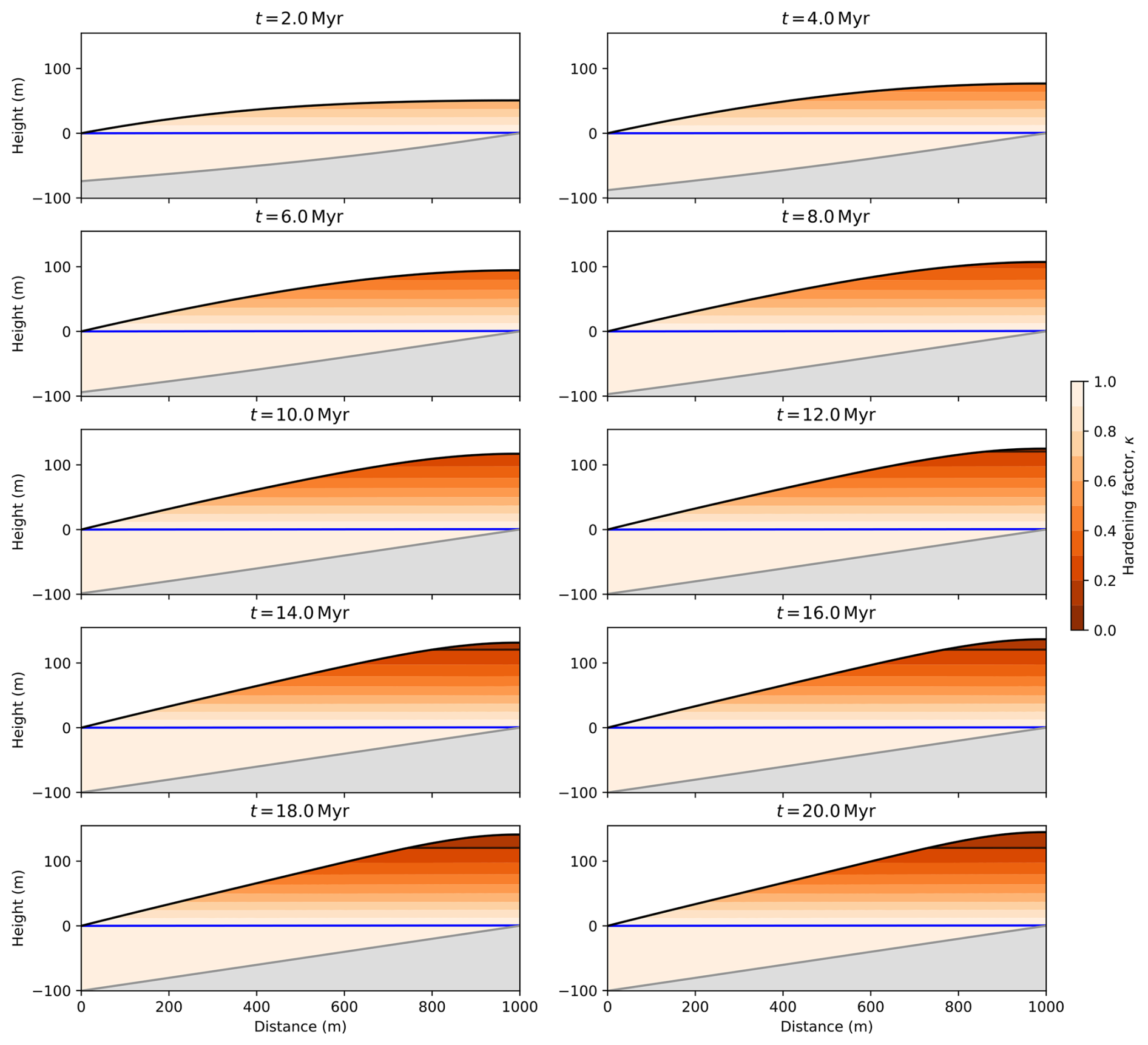
Figure 6 Time evolution of the reference model run (see text for parameter values). Color contours of the hardening parameter, κ. The black line/contour corresponds to the critical value κ = κ_c that defines the formation of a strong duricrust. Steady state is reached at the end of the run.

At the end of the model run, the duricrust is approximately 25 m thick and occupies only the top of the hill. This is a consequence of the assumed percolation mode that restricts the hardening process to the region of the regolith above the water table. The duricrust is sub-parallel to the water table. The small dip is a result of the differential mass loss accompanying duricrust formation.

4.2 Varying τ

Direct or indirect constraints on the value of τ_l for different types of duricrusts have been summarized in Fenske et al. (2025) yielding typical formation times for duricrusts that vary from 10³ to 10⁷ years. In Fig. 7a, we present how the reference model shown in Fig. 6 changes with variations of the time scale of laterisation and mass loss. We also show in Fig. S1, similar results for a broader range of values of τ. We see that a duricrust forms for values of τ smaller than or equal to 4 Myr, which is the value we have used for the reference model. For values of τ > 5 Myr, hardening takes place but κ does not decrease below the critical value κ_c for duricrust formation in the time it takes a rock particle to travel through the regolith layer.

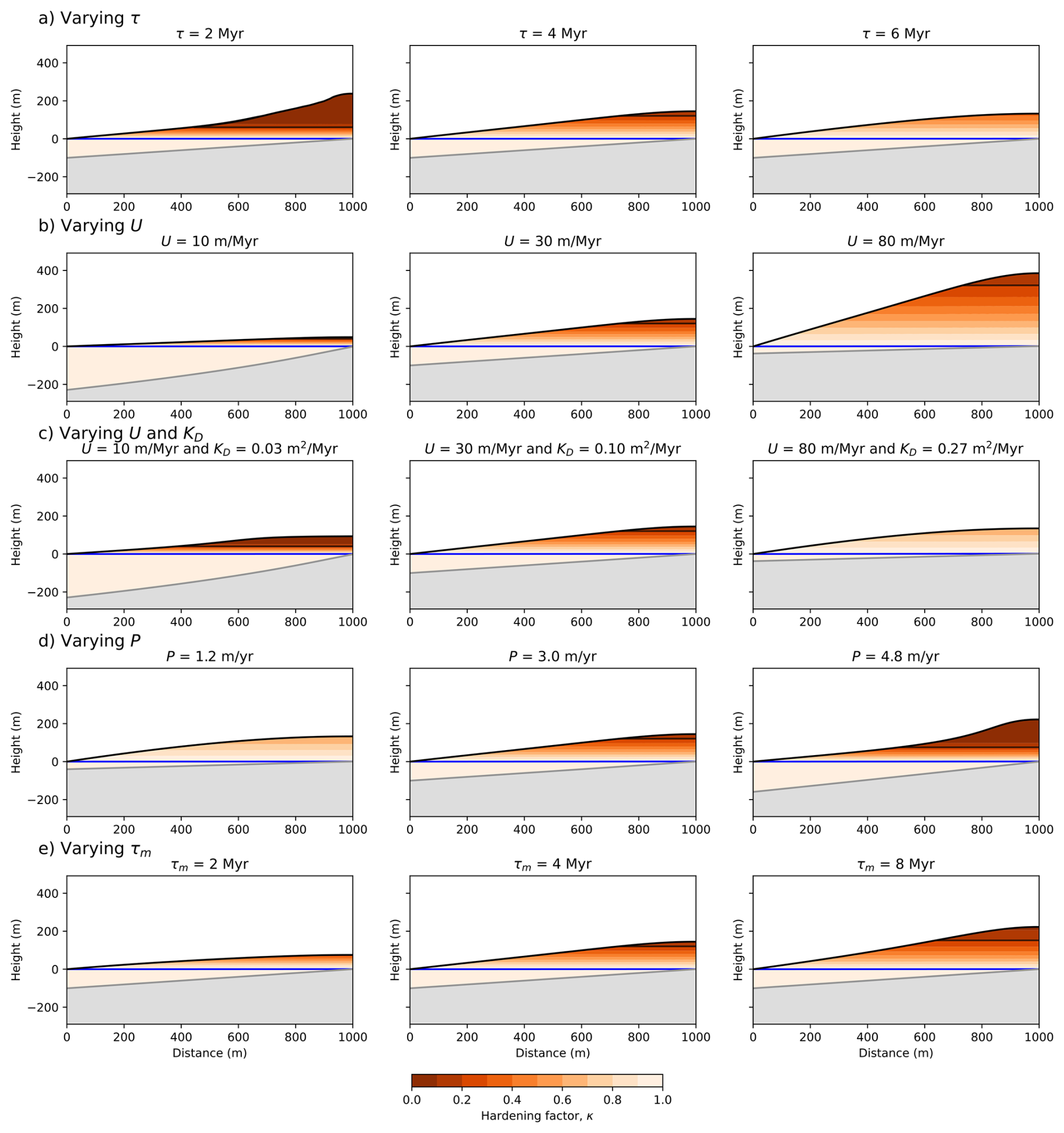
Figure 7 Model behavior in the percolation mode (C = −1) with varying (a) τ, the laterisation and mass loss time scale; (b) U, the uplift rate; (c) U and K_D, the transport coefficient; (d) P, the precipitation rate; and (e) τ_m, the mass loss time scale. Along each row, the three panels correspond to a steady-state solution with increasing value of the parameter. Color contours represent the value of the predicted hardening parameter, κ, and the blue line is the position of the predicted water table.

In cases where a duricrust forms, its thickness varies in inverse proportion to the assumed laterisation time scale. Very small values of τ, lead to unrealistically thick duricrusts forming at the surface of the model. However, with increased hardening, mass loss also increases, resulting in a thinner duricrust (see first two panels in Fig. S1). In all cases, when a duricrust forms, it appears at the top of the hill (where the regolith is thickest). As it thickens, its lateral extent increases too, without affecting the surface topography. Only for an intermediary value of τ < 3 Myr, does the hill surface topography become concave. In all cases where a duricrust forms (small τ values), the regolith thickness beneath the water table is nearly identical to the cases without duricrusts (large τ values), indicating a weak to non-existant feedback between laterisation and primary weathering.

4.3 Varying external forcings, uplift rate U and precipitation rate P

In Fig. 7b, we show the results of a set of experiments in which we have varied the values of the uplift rate U. We also show in Fig. S2, similar results for a broader range of values of U. We see, as described in Braun et al. (2016), that the regolith geometry is a strong function of U. For low values of U, the regolith is thickest near base level (x = 0), and the surface topography (and thus slope) is very low. For high values of U, the regolith is thickest beneath the top of the hill (x = L), and the surface slope is high. This is a direct consequence of the regolith model, independent of the hardening process.

Interestingly, the model predicts the formation of a thin duricrust near the top of the hill, regardless of the value of U. In other words, whether a duricrust forms and, if it does, its thickness relative to the regolith thickness, are independent of the uplift rate, with all other model parameters being kept unchanged. This is because the hill height depends linearly on the uplift rate. Thus the time spent by a rock particle in the regolith (hill height divided by uplift rate) is independent of U. We will develop this point later when deriving a condition for the formation of a duricrust from the hardening equation.

In Fig. 7c, we show model experiments in which we varied the uplift rate, U, and the surface transport coefficient, K_D, in a constant ratio, such that, in the absence of hardening and duricrust formation, the surface slope should be identical in all experiments. We also show in Fig. S3 similar results for a broader range of values of U and K_D.

In this case, duricrusts form only at low uplift rate (U ≤ 30 m Myr⁻¹) and their thickness, as a proportion of the total hill height, increases with decreasing uplift rate. The regolith thickness also increases with decreasing uplift rate, as expected from the model, independently of the hardening process or the formation of a duricrust. Again, there appears to be little to no feedback observed between primary and secondary weathering.

In Fig. 7d, we show the results of a set of experiments with varying precipitation rate, P. We also show in Fig. S4 similar results for a broader range of values of P. We see that hardening happens faster with increased precipitation rate, which can lead to the formation of a duricrust for values of P above 3 m yr⁻¹. Once again, in cases where a duricrust forms, i.e., when κ < κ_c on top of the hill, erosion becomes very inefficient and the hill topography grows at a rate set by the uplift rate, U, corrected by the mass loss rate. The width of the duricrust (i.e., the proportion of the surface of the hill it occupies) appears, however, to be independent of P which leads to the development of a highly concave surface topography.

4.4 Effect of mass loss

In Fig. 7e, we show how varying the mass loss time scale affects the results of the model. We also show in Fig. S5 similar results for a broader range of values of τ_m. In all three model runs shown in Fig. 7e, the laterisation (or hardening) time scale, τ_l has been kept constant at 4 Myr while the mass loss time scale τ_m has been varied as indicated. When mass loss is very efficient, i.e., it takes place on a shorter time scale (τ_m < 4 Myr), the regolith thickness above the water table decreases and the formation of a duricrust is hindered as rock particles do not spend enough time in the regolith for laterisation and hardening to take place. On the contrary, when mass loss occurs on a longer time scale (τ_m > 4 Myr) than laterisation, hardening is amplified and a thicker duricrust develops on top of the profile. This demonstrates the importance of considering mass loss associated with laterisation and leaching for the formation of duricrusts.

4.5 Varying C

In Fig. 8, we show how model parameters and external forcings affect the behavior of the model in the saturated mode (C = 0). In Figs. S6, S7, S8, S9 and S10, we show similar information but for a wide range of laterisation time scales τ_l, uplift rates U, uplift rates U with surface transport coefficients K_D, precipitation rates P and mass loss time scales τ_m, respectively. Note that the reference model has a laterisation time scale value of τ_l = 3 Myr (compared to 4 Myr for the percolation mode).

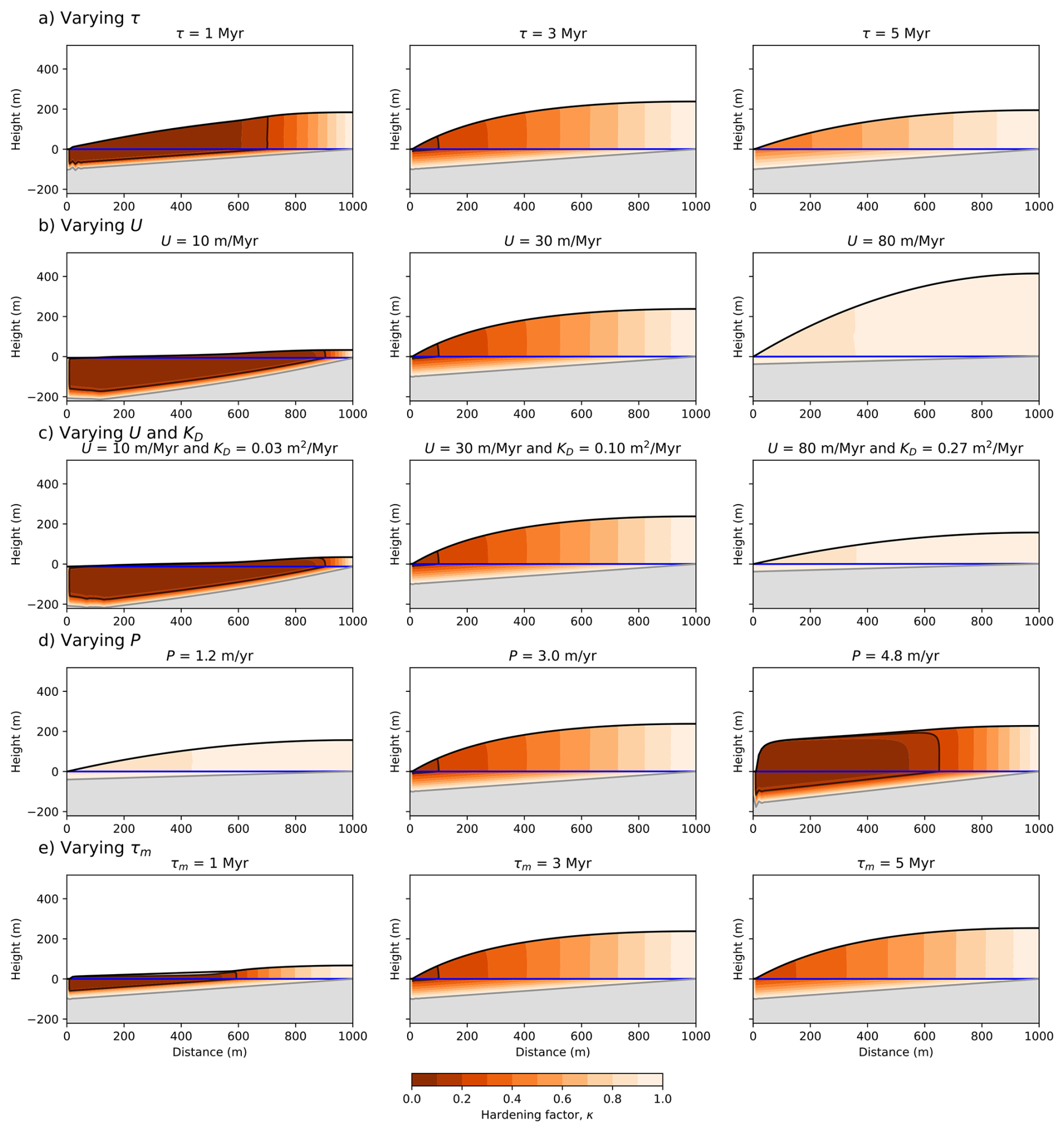
Figure 8 Model behavior in the saturated mode (C = 0) with varying (a) τ, the laterisation and mass loss time scale; (b) U, the uplift rate; (c) U and K_D, the transport coefficient; (d) P, the precipitation rate; and (e) τ_m, the mass loss time scale. Along each row, the three panels correspond to a steady-state solution with increasing value of the parameter. Color contours represent the value of the predicted hardening parameter, κ, and the blue line is the position of the predicted water table.

We see that, in many cases, the main difference with the percolation mode is that, in the saturated mode, hardening takes place below the water table and in the vicinity of the base level (near x = 0). The hardened material is then advected upwards above the water table. In natural settings, strong mass loss could eventually lead to burial of the duricrust by surface sedimentation. Contrary to the percolation mode, the thickness of the duricrust appears to be dependent on the uplift rate, with thicker duricrusts forming at low uplift rate and no duricrust at high uplift rate. Otherwise, like in the percolation mode, decreasing τ, U and K_D simultaneously, or τ_m or increasing P causes the predicted duricrust to be thicker. We also see that, as in the percolation mode, there is little feedback between secondary and primary weatherings, i.e., the thickness of the regolith is not affected by the presence of a duricrust.

In Fig. 9, we show how model parameters and external forcings affect the behavior of the model in the everywhere mode (C = 1). In Figs. S11, S12, S13, S14 and S15, we show similar information but for a wide range of τ_l, U, U with K_D, P and τ_m values, respectively. The reference model for the everywhere mode has a value of τ_l = 5 Myr (compared to 4 Myr in the percolation and 3 Myr in the saturated modes) such that a ≈ 50 m thick duricrust form at the surface of the model after 20 Myr of model evolution. This is because of the longer period spent by rock particles in the laterisation zone, i.e. the entire regolith, which causes faster hardening and thus thicker duricrusts, all other parameters being kept constant.

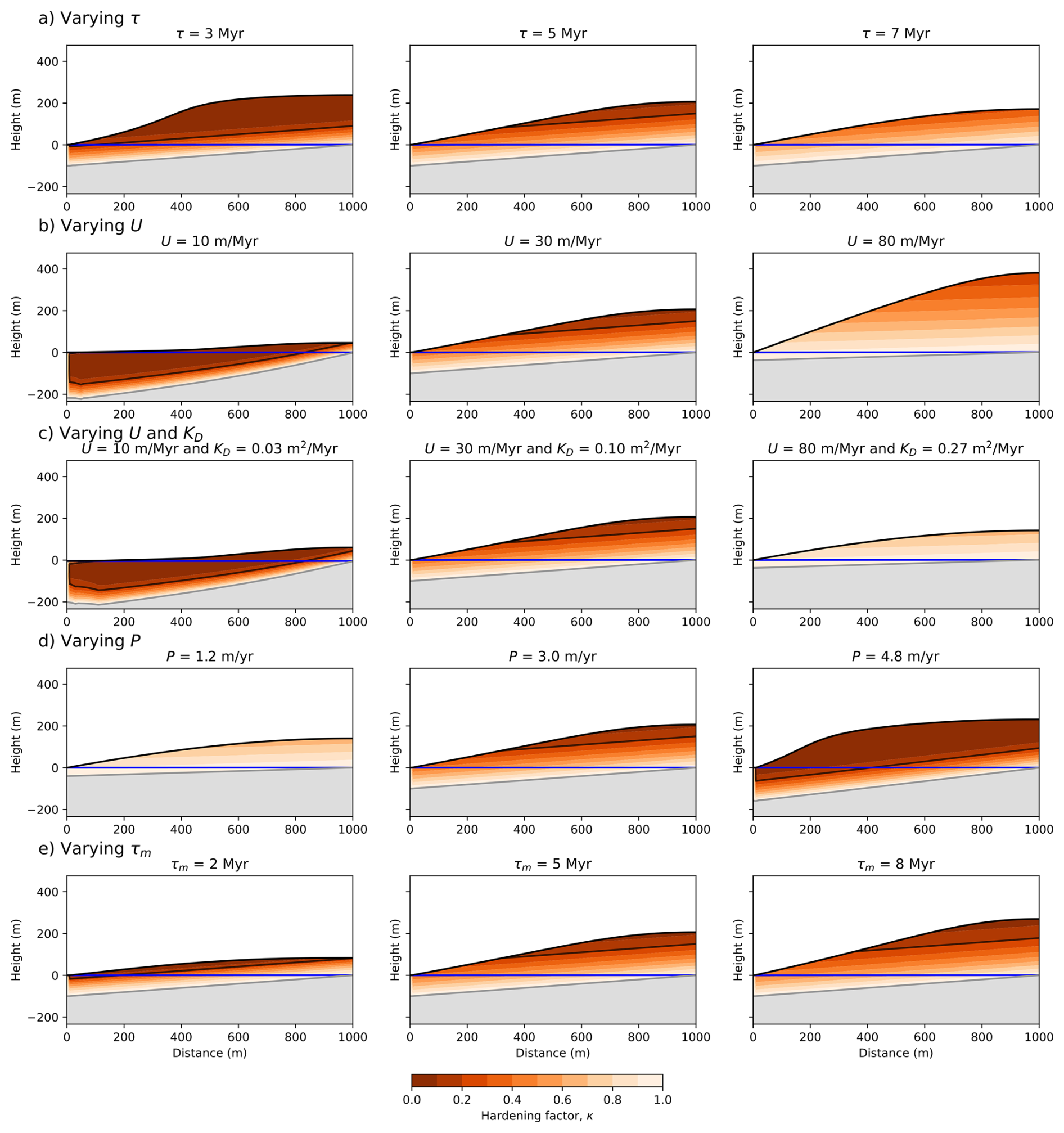
Figure 9 Model behavior in the everywhere mode (C = 1) with varying (a) τ, the laterisation time scale; (b) U, the uplift rate; (c) U and K_D, the transport coefficient; (d) P, the precipitation rate; and (e) τ_m, the mass loss time scale. Along each row, the three panels correspond to a steady-state solution with increasing value of the parameter. Color contours represent the value of the predicted hardening parameter, κ, and the blue line is the position of the predicted water table.

In this mode, when a duricrust forms, it appears first in the middle of the hill, i.e., where the regolith is thickest. Note that this geometry is controlled by the value of the Γ and Ω dimensionless numbers, as described above.

In the everywhere mode, the duricrust thickness (at the end of a 20 Myr long run) increases with decreasing values of τ, U, or U with K_D and increasing values of P. However, in the everywhere mode, the duricrust thickness (and thus the laterisation rate) is relatively independent of the value of the mass loss time scale, τ_m, compared to the dependence on the laterisation time scale τ_l.

4.6 Condition for duricrust formation

We now try to generalize the results obtained above from simple geometric arguments. For this, we consider the distance, h_c, that a rock particle travels through the regolith over a time equal to the laterisation time scale, weighted by the precipitation rate, P, i.e., τ_l × $P/P_{\mathrm{ref}}$. At or near steady-state between uplift and erosion, we can write:

$$\begin{array}{}\text{(13)}& h_{\mathrm{c}}=(U-v_{\mathrm{m}}){\mathit{\tau }}_{\mathrm{l}}{\displaystyle \frac{P_{\mathrm{ref}}}{P}},\end{array}$$

where U is the uplift rate and v_m the mass loss velocity given by:

$$\begin{array}{}\text{(14)}& v_{\mathrm{m}}={\displaystyle \frac{\mathrm{1}}{{\mathit{\tau }}_{\mathrm{m}}}}{\displaystyle \frac{P}{P_{\mathrm{ref}}}}\underset{\mathrm{0}}{\overset{h_{\mathrm{c}}}{\int }}\mathit{\kappa }\mathrm{d}y\approx {\displaystyle \frac{\mathrm{1}}{{\mathit{\tau }}_{\mathrm{m}}}}{\displaystyle \frac{P}{P_{\mathrm{ref}}}}\left(\mathrm{1}+{\mathit{\kappa }}_{\mathrm{c}}\right)h_{\mathrm{c}}/\mathrm{2},\end{array}$$

where κ_c is the critical value of κ at which a duricrust has formed. From this, we can estimate h_c:

$$\begin{array}{}\text{(15)}& h_{\mathrm{c}}={\displaystyle \frac{U{\mathit{\tau }}_{\mathrm{l}}\frac{P_{\mathrm{ref}}}{P}}{\mathrm{1}+\frac{\mathrm{1}+{\mathit{\kappa }}_{\mathrm{c}}}{\mathrm{2}{\mathit{\tau }}_{\mathrm{m}}}}}\end{array}$$

A condition for duricrust formation can be obtained by comparing the regolith thickness (or difference between surface topography z and weathering front height) z−B to h_c. In the percolation mode, maximum regolith thickness above the water table is reached at the hill top, such that z−B = $\frac{U{L}^{\mathrm{2}}}{\mathrm{2}{K}_D}$ − $\frac{UL}{FK}$ (Braun et al., 2016). In the saturated mode, maximum regolith thickness below the water table is reached at the base level, such that z−B = $\frac{FPL}{U}$ (Braun et al., 2016). From the definitions of Ω = $\frac{FKL}{\mathrm{2}{K}_D}$ and of the weathering time scale, τ_w = $\frac{L}{FK}$, we can derive the following condition for duricrust formation in the percolation case:

$$\begin{array}{}\text{(16)}& \mathrm{\Omega }>{\mathrm{\Omega }}_{min}=\mathrm{1}+{\displaystyle \frac{\frac{{\mathit{\tau }}_{\mathrm{l}}}{{\mathit{\tau }}_{\mathrm{w}}}\frac{P_{\mathrm{ref}}}{P}}{\mathrm{1}+\frac{{\mathit{\tau }}_{\mathrm{l}}\left(\mathrm{1}+{\mathit{\kappa }}_{\mathrm{c}}\right)}{\mathrm{2}{\mathit{\tau }}_{\mathrm{m}}}}}.\end{array}$$

For the saturated case, we make use of Ω = $\frac{FKS}{U}$ and Γ = $\frac{K{S}^{\mathrm{2}}}{P}$ to obtain:

$$\begin{array}{}\text{(17)}& \mathrm{1}+{\displaystyle \frac{{\mathrm{\Omega }}^{\mathrm{2}}}{\mathrm{\Gamma }}}>{\mathrm{\Omega }}_{min}=\mathrm{1}+{\displaystyle \frac{\frac{{\mathit{\tau }}_{\mathrm{l}}}{{\mathit{\tau }}_{\mathrm{w}}}\frac{P_{\mathrm{ref}}}{P}}{\mathrm{1}+\frac{{\mathit{\tau }}_{\mathrm{l}}\left(\mathrm{1}+{\mathit{\kappa }}_{\mathrm{c}}\right)}{\mathrm{2}{\mathit{\tau }}_{\mathrm{m}}}}}.\end{array}$$

We can verify these condition by performing a large number of numerical experiments varying U (uplift rate), P (precipitation rate), and τ (time scales). The results are shown in Fig. 10a as contour plots of the minimum predicted hardening parameter at steady-state as a function of the assumed precipitation rate, P, and uplift rate, U, values for a range of laterisation and mass loss time scales, τ. On each panel, we also show the contour value corresponding to the critical hardening parameter for duricrust formation, κ_c = 0.2 (white solid line) as well as the prediction from the threshold analysis (Eqs. 16 and 17, dashed white line). We see that the two lines are very close to each other implying a good agreement between theory and numerical model results. This result also validates our numerical implementation of the algorithm.

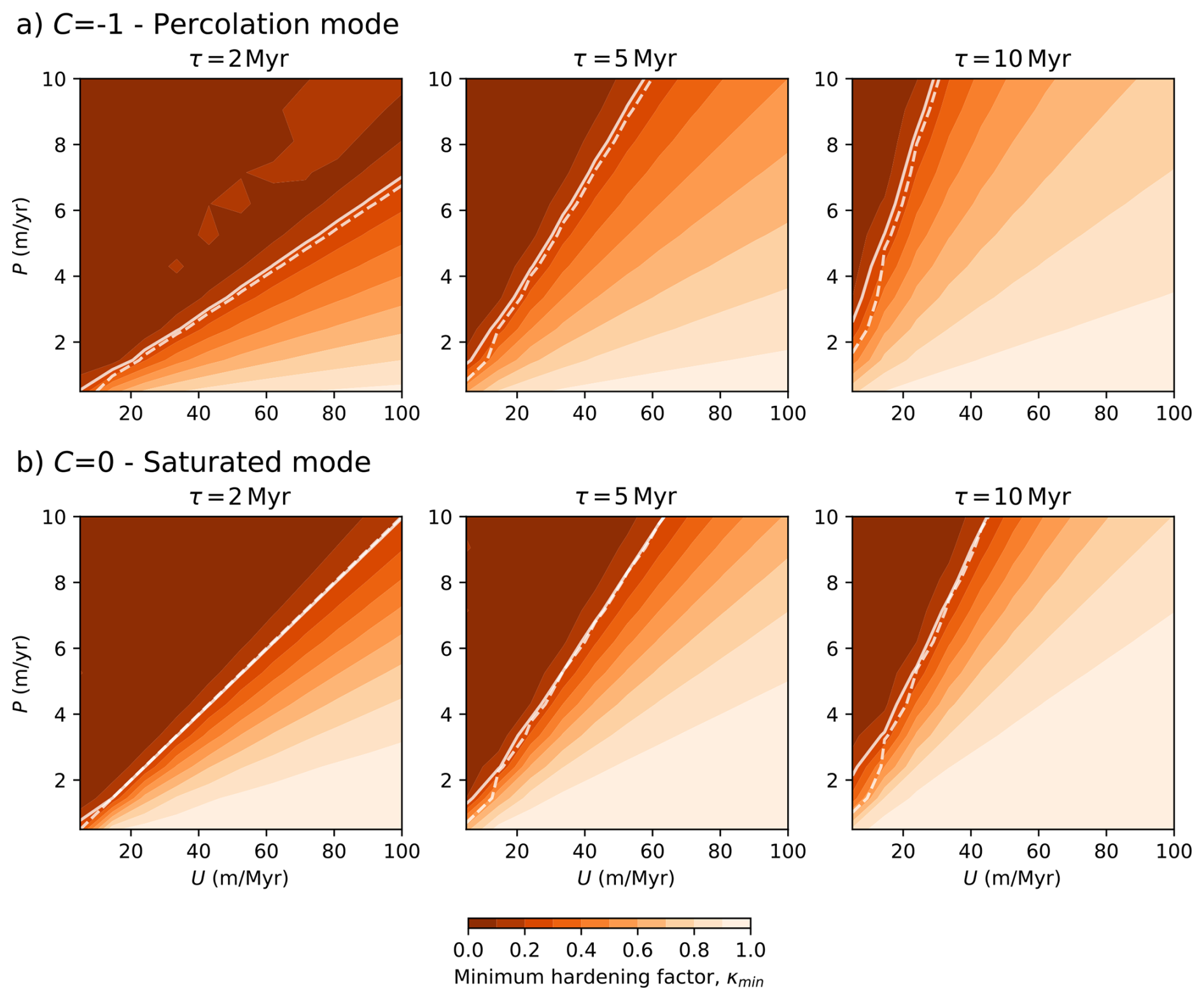
Figure 10 Contours of minimum hardening factor values (κ) as a function of uplift rate (U) et precipitation rate (P) for different values of the laterisation time scale (τ) and weathering modes (C). White line corresponds to the κ = 0.2 value and white dashed line to the prediction of Eqs. (16) and (17).

It is also interesting to consider the asymptotic behavior of Ω_min as a function of τ_m:

$$\begin{array}{}\text{(18)}& \underset{{\mathit{\tau }}_{\mathrm{m}}\to \mathrm{0}}{lim}{\mathrm{\Omega }}_{min}=\mathrm{1}\text{and}\underset{{\mathit{\tau }}_{\mathrm{m}}\to \mathrm{\infty }}{lim}{\mathrm{\Omega }}_{min}=\mathrm{1}+{\displaystyle \frac{{\mathit{\tau }}_{\mathrm{l}}}{{\mathit{\tau }}_{\mathrm{w}}}}{\displaystyle \frac{P_{\mathrm{ref}}}{P}}\end{array}$$

demonstrating that if mass loss is extremely rapid (τ_m arrows zero) the regolith and thus any duricrust will be very thin or non-existent, while, if there is no mass loss, the criterion for duricrust formation is only function of the ratio of laterisation time scale to weathering time scale (or time scale for secondary to primary weathering). This explains the relatively strong dependence of the solution (presence of a duricrust) on the mass loss time scale.

4.7 Periodic variations in uplift rate

We now present model simulations in which we have varied the uplift rate in a periodic fashion, simulating a tectonic setting made of phases of active uplift followed by periods of tectonic quiescence, of equal length, T. This setup is similar to the one we used in Fenske et al. (2025) to illustrate the behavior of the model for duricrust formation by water table fluctuations (WTF model). In the results shown in Fig. 11, the uplift rate varied between 0 (quiescence) and 50 m Myr⁻¹ (active uplift) every 4 Myr for a total model duration of 40 Myr. Each row in Fig. 11 therefore corresponds to a complete cycle of tectonic uplift followed by quiescence. All model parameters are identical to those used in the reference model, such that the period of the tectonic signal (4 Myr) is equal to the laterisation time scale, τ. The experiment is performed in the percolation mode (C = −1). We see that during each period of uplift, the surface topography increases, but little hardening takes place. During the phases of quiescence, hardening takes place but only above the water table. The surface topography is eroded and the regolith thickens. During the subsequent period of uplift, the hardened layer, i.e. the duricrust, is uplifted together with the surrounding material.

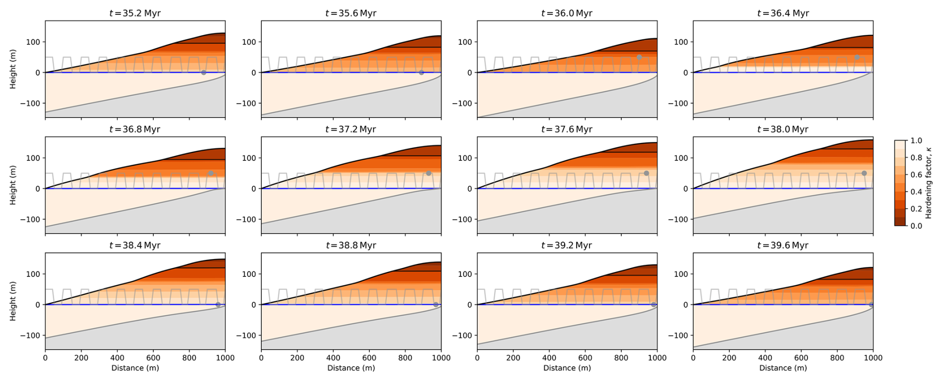
Figure 11 Varying the uplift rate by introducing periods of quiescence (U = 0) and active uplift (U = 60 m Myr⁻¹) of equal duration, 4 Myr. All model parameters are identical to those of the reference model in the percolation mode. The circle on the thin grey line shows the position of the corresponding panel with respect to the uplift cycles.

The same simulation, using the percolation mode, was performed with a set τ = 1.2 × 10⁸ years to generate a landscape without duricrust formation. In Fig. 12, we compare the resulting topographies of both scenarios to illustrate the influence of duricrusts on the regolith column. During each uplift cycle, the duricrusted topography attains higher elevations than the regolith-only topography, although the difference in height remains minimal. The quiescent period induces more intense erosion on the regolith-only hill, while duricrust formation occurs on the other, and the resulting topography withstands erosion. We see that the topography difference between both scenarios is at its highest during that part of the simulation. These results show that duricrusts provide a degree of protection against erosion, although to a limited extent.

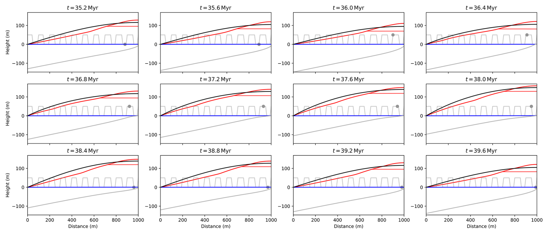
Figure 12 Comparison of contours for the percolation mode (in red) and a scenario without duricrust formation (in black). The water table (in blue) and weathering front (in gray) are the same for both scenarios. The varying uplift rate is the same as for the previous scenario. All model parameters are identical to those of the reference model in the percolation mode, apart for τ in the scenario without duricrust formation, with τ = 1.2 × 10⁸. The circle on the thin grey line shows the position of the corresponding panel with respect to the uplift cycles.

A similar experiment in the saturated mode (C = 0), but with a period equal to 5 Myr, yields rather different results (Fig. 13). During each cycle of quiescence, a discrete duricrust forms. The resulting growing collection of duricrusts is then advected upwards above the water table and exposed to surface erosion. This results from the combined action of regolith thickening and laterisation-driven mass loss below the water table that creates a cycle of up-and-down motions for each duricrust. Near the base level, the cycles combined to form a single highly resistant duricrust, but away from base level, the duricrusts are clearly distinct. They all dip parallel to the direction of the weathering front, crossing both the water table and the surface topography. The thick duricrust that forms near base level is highly resistant to erosion but the thinner duricrusts that radiate from it are less resistant, causing the hill to develop a ramp-flat geometry that grows with time. This result demonstrates the importance of considering mass loss associated with laterisation, especially in the saturated mode. For completeness we show in Fig. S16 similar results obtained in the everywhere mode.

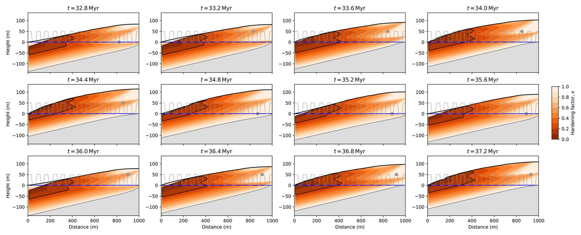
Figure 13 Varying the uplift rate by introducing periods of quiescence (U = 0) and active uplift (U = 60 m Myr⁻¹) of equal duration, 5 Myr. All model parameters are identical to those of the reference model in the saturated mode. The circle on the thin grey line shows the position of the corresponding panel with respect to the uplift cycles.

4.8 Periodic variations in precipitation rate

In Figs. 14 and 15, we show results similar to those shown in Figs. 11 and 13 but in which we vary the precipitation rate, P, in a periodic fashion, between 0.5 and 7.5 m yr⁻¹. The resulting geometries are quite similar: in the percolation mode, laterisation and the growth of a surface duricrust take place during the wet periods only. During the dry period, the duricrust is eroded away at the surface. In the saturated mode, several families of duricrusts can be observed to form in the regolith. Cycles involve the formation and growth of a duricrust beneath the water table during wet periods, and its vertical advection towards the surface and erosion during dry periods. In both modes, the regolith thickness increases during wet periods and decreases during dry periods. For completeness, we show the results of a similar experiment performed in the everywhere mode in Fig. S17.

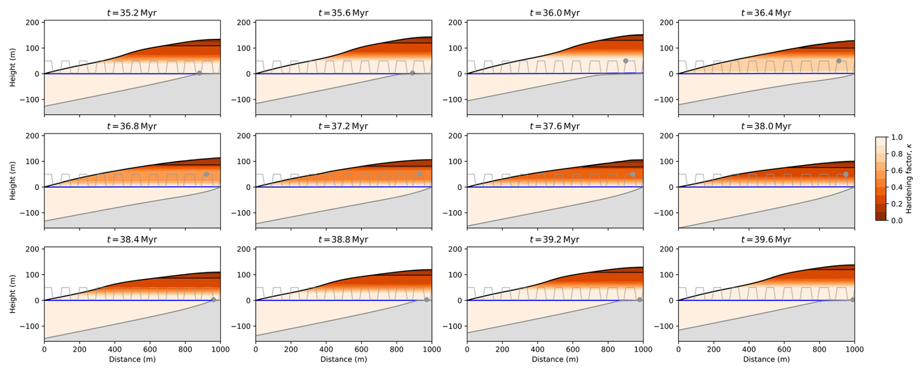
Figure 14 Varying the precipitation rate by introducing dry (P = 0.5 m yr⁻¹) and wet periods (P = 7.5 m yr⁻¹) of equal duration, 4 Myr. All model parameters are identical to those of the reference model in the percolation mode. The circle on the thin grey line shows the position of the corresponding panel with respect to the uplift cycles.

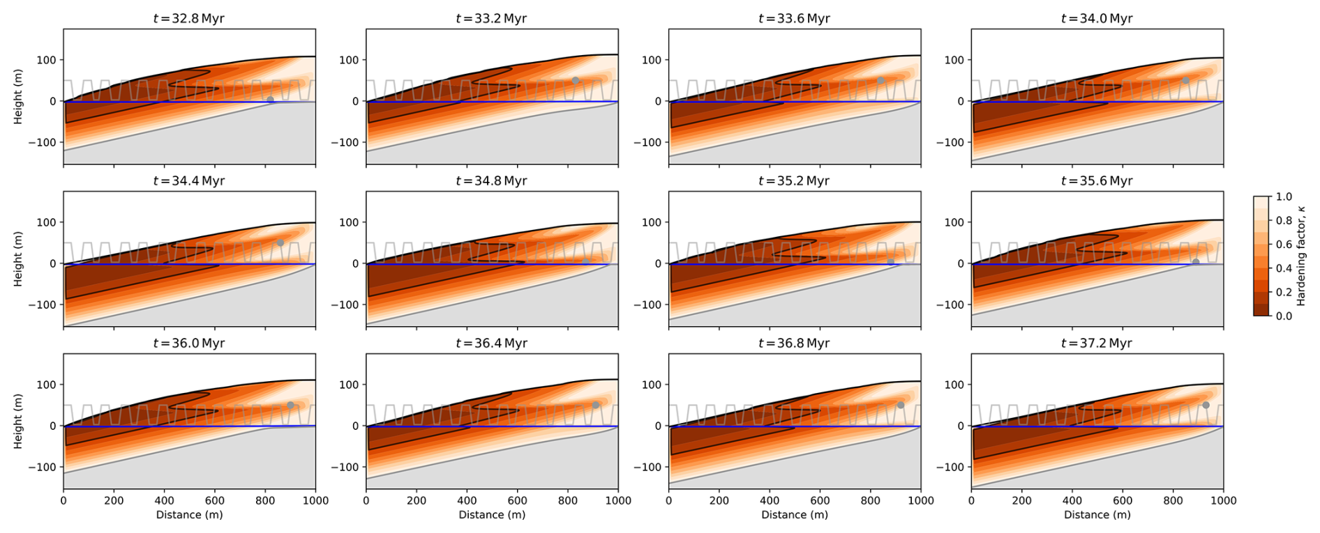
Figure 15 Varying the precipitation rate by introducing dry (P = 0.5 m yr⁻¹) and wet periods (P = 7.5 m yr⁻¹) of equal duration, 5 Myr. All model parameters are identical to those of the reference model in the saturated mode. The circle on the thin grey line shows the position of the corresponding panel with respect to the uplift cycles.

4.9 Predicting ages

As explained in the method section, we can use the model to predict the age of primary weathering, i.e., the time since a regolith particle crossed the weathering front as well as a secondary weathering (or hardening) age, i.e., the time it was affected by laterisation and thus hardening. In Fig. 16 we show contours of mean duricrust ages (left panel), plots of mean and standard deviation of duricrust age (blue circles) and weathering age (red circle) as a function of position along a vertical profile (center panel), and along the surface of the model (right panel) for three model runs characterized by different modes, i.e., (a) percolation, (b) saturated and (c) everywhere modes. We also show distributions or spectra of ages for all points along the profiles (beige shaded area). The distributions computed along the vertical profiles and used to compute the mean and standard deviations of the ages shown in the central panel are given in Fig. S18.

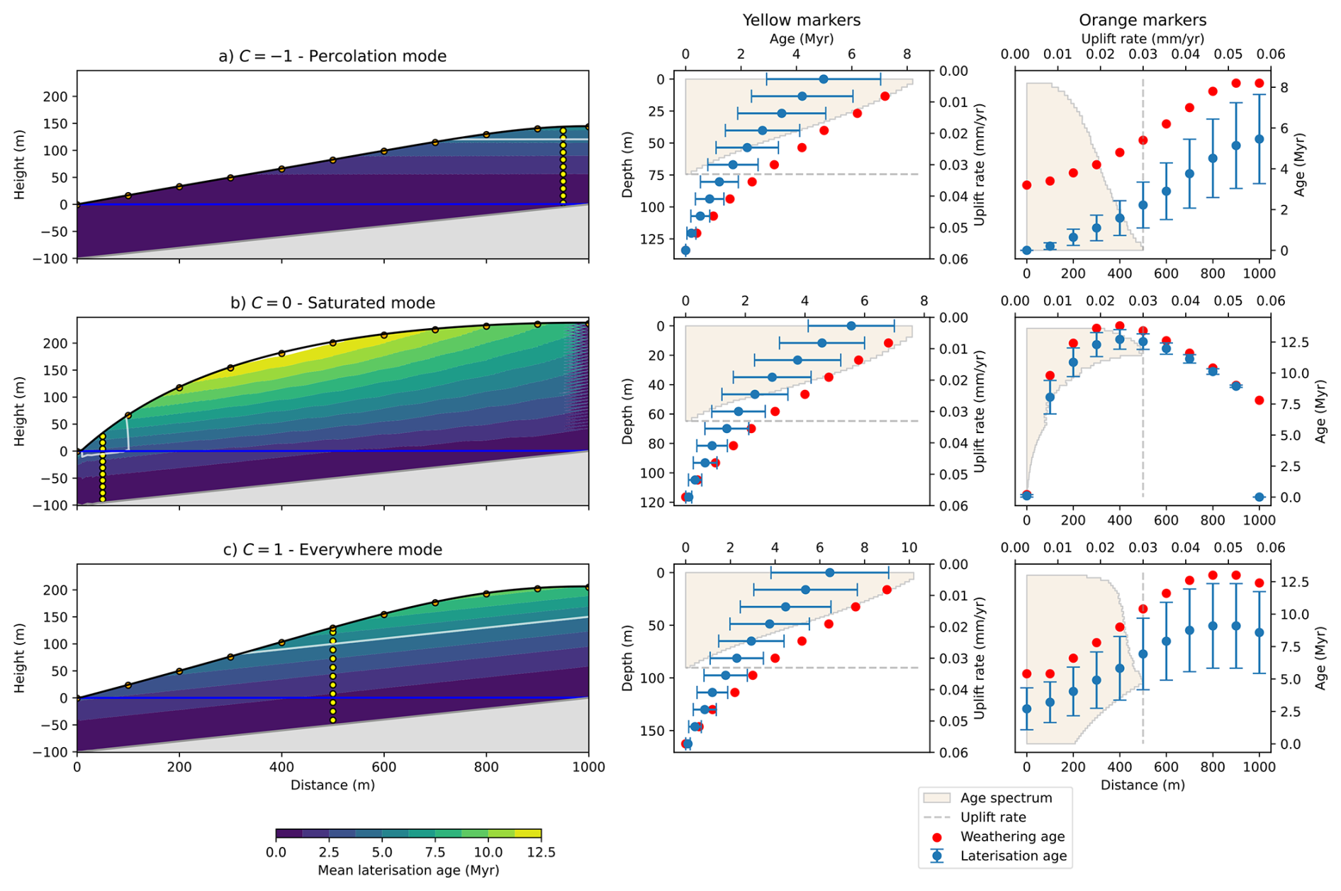
Figure 16 Contours of secondary weathering ages (left panels) for experiments in (a) the percolation, (b) the saturated and (c) the everywhere modes. The white lines outline duricrusts. Central panels show distribution of mean and standard deviation in secondary weathering ages (blue circles) and primary weathering ages (red circles) along a vertical profile shown in the left panel. Beige shaded area is the computed distribution of ages for the entire profile. Right panel is similar to central panel but for points located along the surface of the model.

The model runs shown in Fig. 16 have model parameters identical to the reference model experiments in the percolation (with τ = 4 Myr), saturated (with τ = 3 Myr) and everywhere (τ = 5 Myr) modes. In each experiment, the position of the vertical profile has been selected so that it crosses the duricrust.

We see that both the primary and secondary weathering ages increase from bottom to top. The rate of increase of primary weathering ages with distance to the base of the regolith (weathering front) is set by the uplift rate (here 30 m Myr⁻¹). The rate of increase of the mean secondary weathering age with distance from the weathering front is approximately half of it. This is because secondary weathering is a continuous process that always affects all parts of the profile. This also explains why the standard deviation in secondary weathering ages is largest near the surface. Indeed, a point that is close to the surface has experienced secondary weathering throughout its journey through the regolith and has therefore accumulated ages ranging from the time it crossed the weathering front to the present. This is also reflected in the very skewed distribution of ages (shaded areas in central and right panels of Fig. 16) with a strong bias towards young ages which can be found at all depths in the profiles. These characteristics of age distribution with depth are common to all three modes (a to c in Fig. 16). They are also observed in many natural age profiles (Monteiro et al., 2014; Vasconcelos and Carmo, 2018; Heller et al., 2022).

Interestingly, the surface age profiles (right panels in Fig. 16) are different in the three modes, with both the primary and mean secondary ages showing a maximum where the regolith profile is thickest. The standard deviation in secondary weathering ages varies strongly in both the percolation and the saturated modes due to the lack of young ages in the percolation mode and old ages in the saturated mode.

4.9.1 Age predictions under periodic settings

In Fig. 17 we show computed ages for a series of model runs in which we varied the uplift rate in a periodic manner. All model parameters are those of similar runs presented in Sect. 4.7. The period of uplift oscillations equal to the laterisation time scale, i.e., T = 4, 3 and 5 Myr in the cases C = −1, 0 and 1, respectively.

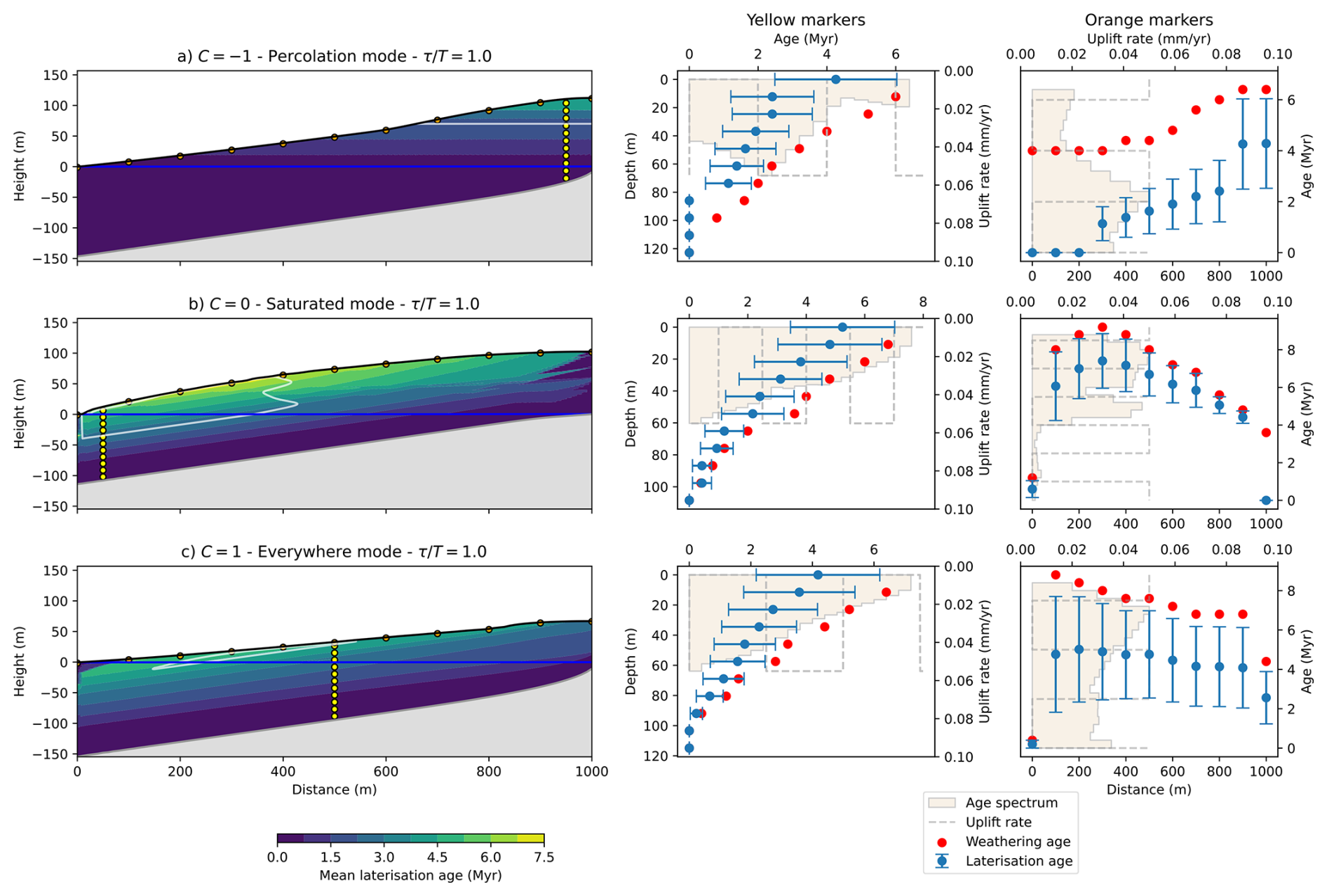
Figure 17 Age predictions for three model experiments with periodic variations in uplift rate. See Fig. 16 for detailed description of figure. The dashed lines in the central and right panels indicate the periods of active uplift. T is the period of the uplift function.

We see that the predictions are very similar to those of the runs with constant uplift rate presented above except for the breaks in the age-depth profiles (central panels) and the age distributions/spectra. The breaks in the primary weathering age-depth profiles (red circles) take place at the time of change in uplift rate. However, there is no clear pattern with some changes causing greater break in slopes than others. The age spectra (beige shaded area) display several peaks but they are difficult to correlate to periods of active uplift or tectonic quiescence. This shows that age distributions can be used to constrain the evolution of uplift in a given setting but that the interpretation is not straightforward. This results from the complex evolution of a system subject to periodic uplift rate variations. A change in uplift rate strongly affects the velocity at which a particle traverses the regolith and thus the rate at which it hardens and accumulates ages during a given set period. But changing the uplift rate also affects the rate of downward propagation of the weathering front into the bedrock and thus the thickness of the regolith.

The mean and standard deviation ages along the surface display the same pattern with older ages found where the duricrust is exposed. The age distributions also show several peaks but they are difficult to relate directly to the uplift history, i.e., whether the peaks correspond to periods of uplift activity and/or quiescence.

In Fig. 18, we show the age predictions for a series of model experiments in which we varied the precipitation rate in a periodic fashion, similar to those presented in Sect. 4.8. The value of the period (equal to the laterisation time scale) has been adapted to each mode (i.e., T = 4, 3 or 5 Myr for C = −1, 0 and 1).

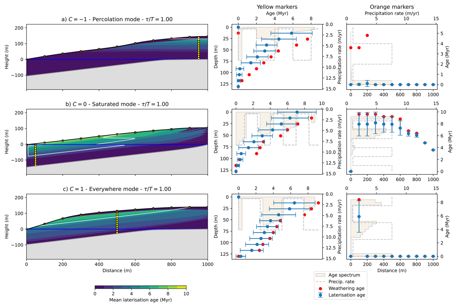
Figure 18 Age predictions for three model experiments with periodic variations in precipitation rate. See Fig. 16 for detailed description of figure. The dashed lines in the central and right panels indicate the periods of enhanced precipitation rate. T is the period of the precipitation function.

The patterns of predicted ages are, in general, easier to interpret with breaks in slopes of age-elevation profiles clearly associated with periods of reduced rainfall (dry periods). Predicted distributions also display well defined peaks that correspond to the wet periods. This implies that if clear peaks appear in age distributions, they are most likely due to variations in precipitation rate. We have to keep in mind, however, that this result is a direct consequence of the hypothesis that we have built into the model that laterisation is linearly proportional to precipitation rate.

4.10 Physical vs. chemical fluxes

In Fig. 19, we show ratios of the chemical over physical fluxes, ϕ_C $/$ ϕ_P, as a function of the mass loss time scale, τ_m, in the three laterisation modes. As expected, we see that, in all cases, the relative importance of the chemical flux decreases with the ratio τ_m $/$ τ_l. This is because the efficiency of mass loss is directly proportional to the value of τ_m. Interestingly, chemical and physical erosions appear to be equally efficient (ϕ_C $/$ ϕ_P ≈ 1) when the mass loss time scale is approximately equal to the laterisation time scale (τ_m $/$ τ_l ≈ 1).

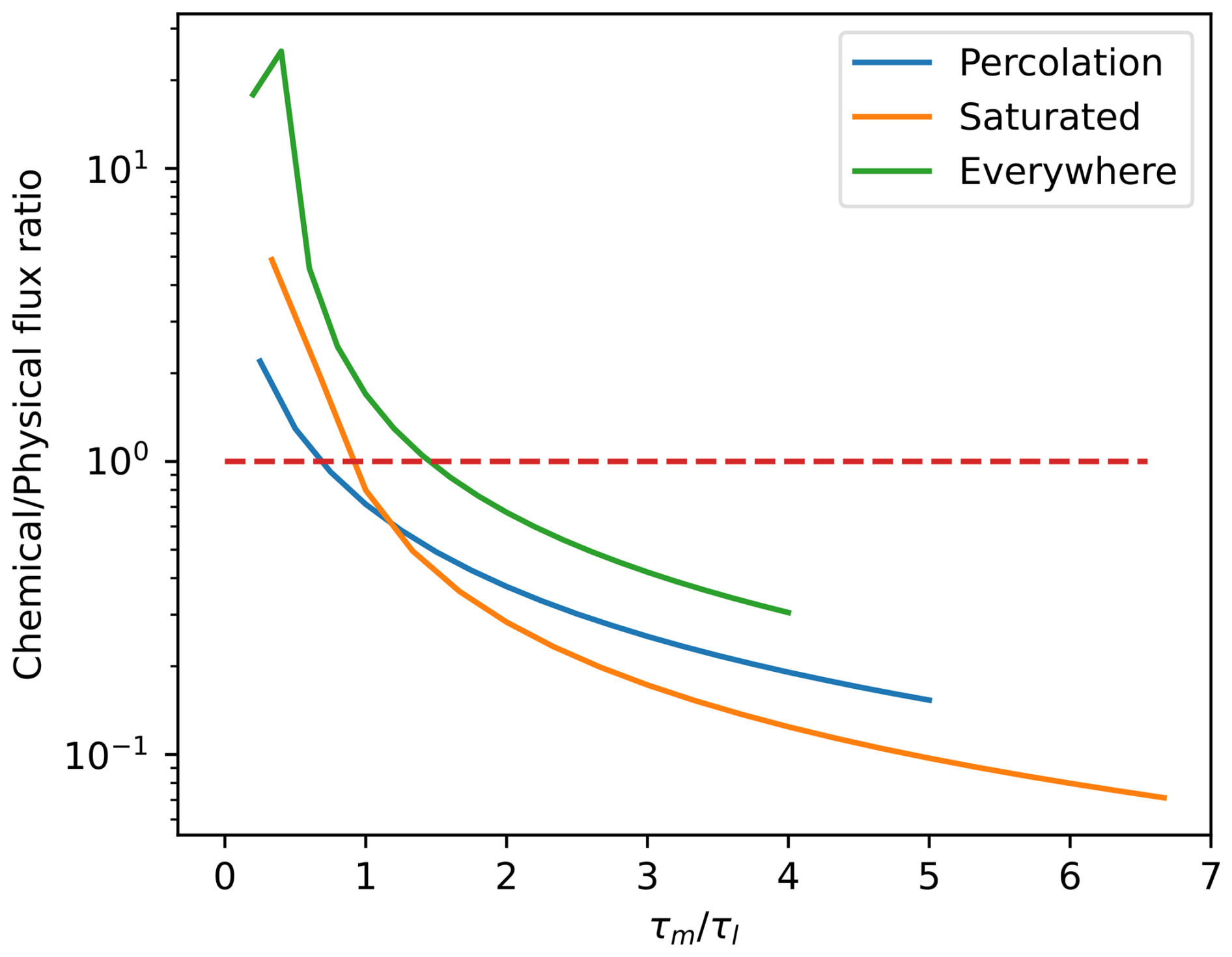
Figure 19 Computed ratio of chemical vs. physical fluxes (or erosion rate) as a function of the ratio of the mass loss time scale and the laterisation time scale. Values estimated at the end of a model run in which the time scale for laterisation, τ_l, was chosen to lead to the formation of a thin duricrust (i.e, τ_l = 4, 5 and 7 Myr in the percolation, saturated and everywhere modes, respectively).

In Figs. 20 and 21, we show computed physical and chemical fluxes out of the model as a function of time, for some of the model runs in which we vary the uplift or precipitation rate in a periodic fashion. Variations in uplift rate (Fig. 20) generally lead to an increase in both physical and chemical fluxes during periods of enhanced uplift rate, in comparison to the tectonically more quiet periods. This pattern is inverted, however, in the saturated mode (panels b, e and h in Fig. 20). In these model runs, even though it represents only 10 % of the total flux, the contribution from chemical weathering increases during the more quiet periods. This is because the regolith layer thickness increases by deepening of the weathering front during periods of decreased uplift rate, which, in turn, increases the size of the region where secondary (chemical) weathering takes place, i.e., below the water table. On the contrary, in the percolation mode, this downward migration of the weathering front does not contribute to increasing the secondary weathering rate, which is limited to the region above the water table. In the percolation model, this region experiences thinning during periods of reduced uplift rate in response to the lowering of the surface topography.

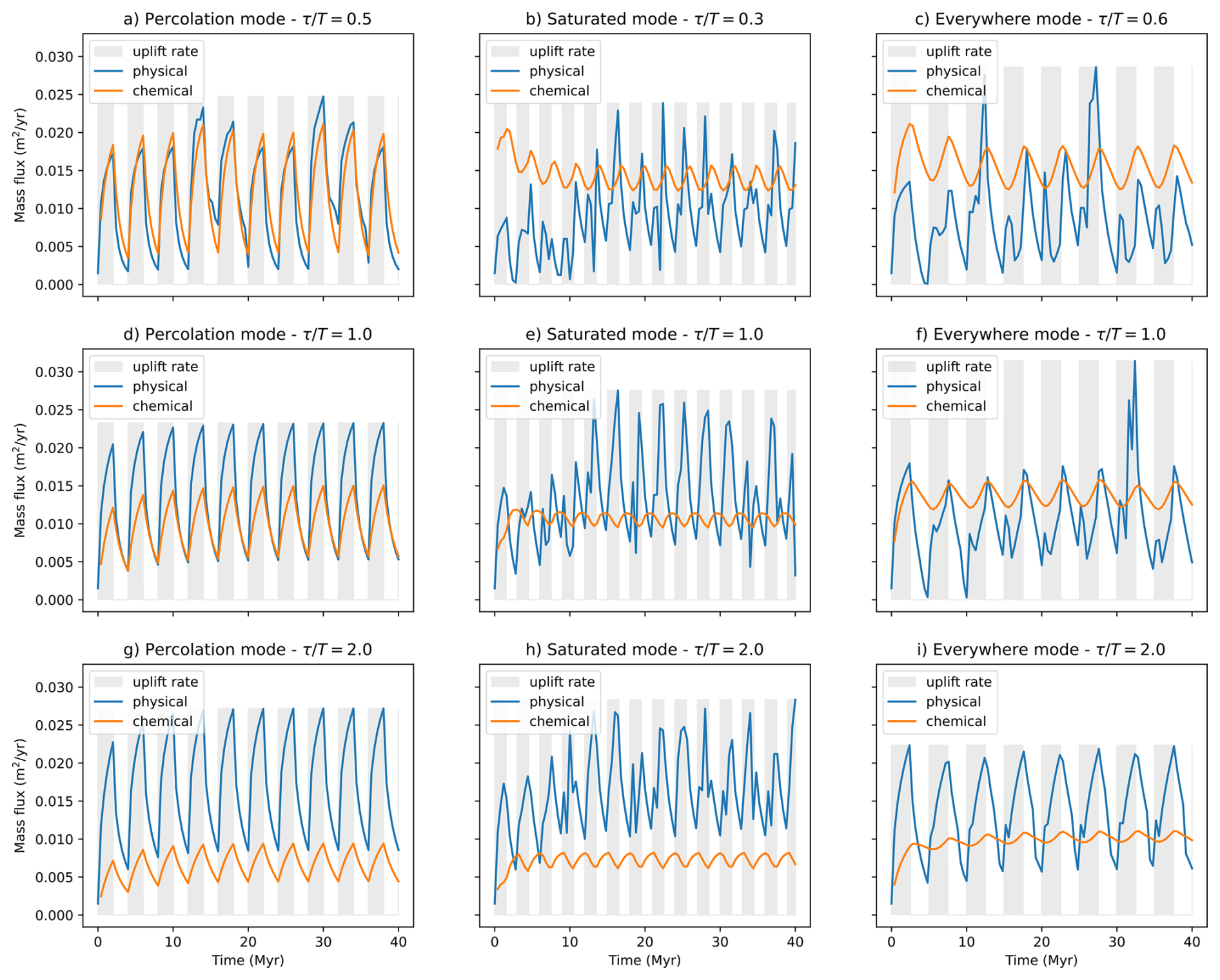
Figure 20 Predicted variations in chemical and physical fluxes as a function of time for model run experiments with periodic uplift rate. Each column corresponds to a different mode (C) and each row to a different ratio of the laterisation time scale (τ) by the period (T). Note that, as in model experiments shown in Figs. 11 and 13, in each mode, the period of forcing was selected to be equal to the laterisation time scale that lead to the formation of a thin duricrust, i.e., T = 4, 4 and 7 Myr, respectively. Grey shaded areas indicate periods of enhanced uplift rate.

In the model runs where precipitation rate varies periodically (Fig. 21), we see that the two fluxes are varying in opposite directions, with the chemical flux increasing during the wet periods and the physical flux increasing during the dry periods. This is because during wet periods the rate of laterisation increases (due to the precipitation dependence built in our model – Eq. 5) which causes higher chemical flux through enhanced mass loss. This mass loss leads to a lowering of the surface topography and slope, and, consequently, a reduced efficiency of the physical erosion where transport is linearly proportional to slope.

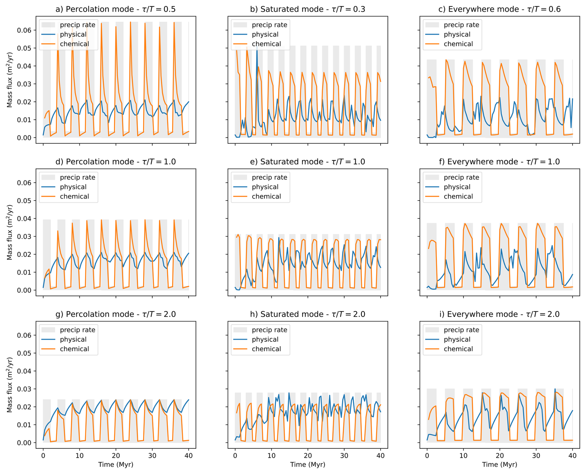
Figure 21 Predicted variations in chemical and physical fluxes as a function of time for model runs experiments with periodic precipitation rate. Each column corresponds to a different mode (C) and each row to a different ratio of the laterisation time scale (τ) by the period (T). Note that, as in model experiments shown in Figs. 14 and 15, in each mode, the period of forcing was selected to be equal to the laterisation time scale that lead to the formation of a thin duricrust, i.e., T = 4, 4 and 7 Myr, respectively. Grey shaded areas indicate periods of enhanced precipitation rate.

5 Discussion

5.1 Constraints on duricrust formation time τ

In Fenske et al. (2025), we compiled a comprehensive dataset of various duricrust formation rates inferred from volumetric calculations (Leneuf, 1959; Trendall, 1962; Goudie, 1973; Wright, 1989; Boulangé, 1984; Paquet and Clauer, 1997; Boulangé et al., 1997; Tardy and Roquin, 1992; Tardy, 1969; Horbe and Anand, 2011; Momo et al., 2020; Chen et al., 1988; Taylor and Eggleton, 2001; Fritz and Tardy, 1973; Goudie, 1985) and geochronological data (Gac, 1980; Hénocque et al., 1998; Théveniaut and Freyssinet, 1999; Vasconcelos and Conroy, 2003; Théveniaut et al., 2007; Vasconcelos and Carmo, 2018; dos Santos Albuquerque et al., 2020; Netterberg, 1978; Candy et al., 2003; de Oliveira Carmo and Vasconcelos, 2006; Dhir et al., 2010; Heller et al., 2022) spanning the past 70 years of research. This analysis reveals that the formation time for a 1 m-thick duricrust ranges from approximately 10 kyrs to 10 Myrs.

Furthermore, it is important to note that the formation rate is highly dependent on the duricrust and bedrock types. For example, a 1 m-thick calcrete develops more rapidly than a ferricrete (Fenske et al., 2025), and an iron-poor carbonate bedrock will lead to slower accumulation of ferruginous minerals than on Banded Iron Formations (BIFs, i.e. sedimentary rocks alternating iron rich layers with iron poor layers. The iron content is at least 15 %). Thus, utilising the duricrust formation model in concert with data, it will be important to adjust τ accordingly. We suggest following orders of magnitude:

• For pedogenic calcretes: 1 × 10⁴ to 1 × 10⁵ years;

• For pedogenic silcretes: 1 × 10⁶ years;

• For ferricretes: 1 × 10⁵ to 1 × 10⁷ years;

• For bauxitic duricrusts and alcretes: 1 × 10⁶ years.

In accordance with these observations, the values of the model parameters τ_m and τ_l, that we used in the model experiments presented above, i.e. 1–10 × 10⁶ years, should be regarded as representative for the formation of alcretes and ferricretes.

Note also that, because τ appears in the expression for Ω_min, its value will affect not only the rate of duricrust formation but also the conditions under which a duricrust will develop. In turn, this implies that different types of duricrusts are likely to form under different climatic and tectonic conditions. It is commonly assumed that calcretes form in more arid conditions compared to bauxitic duricrusts that form in more wet, tropical conditions (e.g. Goudie, 1985; Tardy, 1993; Webb and Nash, 2020).

5.2 Conditions for the formation of regolith and duricrust

According to the regolith model we have used (Braun et al., 2016), the presence of a regolith layer at the Earth's surface depends on whether the value of a dimensionless number Ω, equal to the ratio between the erosion time scale (τ_e) and the primary weathering time scale (τ_w), exceeds unity or not. We have shown here that the formation of a duricrust requires that Ω be larger than unity plus a term that depends on the ratio between the secondary (τ_l) and primary (τ_w) weathering time scales (Eq. 16). This implies that duricrusts form more readily in situations where the secondary weathering time scale is much shorter than the primary weathering time scale. We can summarize this finding by stating that an environment in which duricrusts are likely to form is characterized by the following inequalities:

$$\begin{array}{}\text{(19)}& {\mathit{\tau }}_{\mathrm{l}}<{\mathit{\tau }}_{\mathrm{w}}<{\mathit{\tau }}_{\mathrm{e}}\end{array}$$

i.e., the time scale for secondary weathering, τ_l, must be smaller than the time scale for primary weathering, τ_w, which, in turn must be smaller than the erosion time scale, τ_e.

Although these relationships were derived assuming a steady-state system, they can be used to estimate how, i.e., in which direction, regolith and duricrust thickness and hardness evolve in a transient system.

5.3 Mass loss and the geometry of duricrusts

Mass loss is caused by leaching, identified as the main process for material to leave the system during laterisation (Tardy, 1993). When material is leached away, porosity increases in the remaining system. As a result, the system collapses under gravity, which results in volume loss. Some authors (e.g. Taylor and Eggleton, 2001) mention landscape lowering associated with laterisation, which can be associated to volume loss. However, due to lack of data, statistically quantifying mass loss rate like we did for different weathering rates in Fenske et al. (2025), is not possible. Decoupling mass loss from hardening is, however, plausible as hardening is caused by the removal of soluble (and softer) components of the regolith during secondary weathering, but there is no well-defined relationship between material removal (and thus mass loss) and hardening. It is most likely that hardening takes place in the late stages of leaching, and thus τ_m is likely to be smaller than τ_l, but it does not have to be the case. In fact, the composition of the bedrock is likely to exert strong influence on the ratio τ_m $/$ τ_l, especially through the initial concentration in the most resistant elements (iron, for example). An iron-rich bedrock will lead to formation of a ferricrete with relatively less mass loss than an iron-poor bedrock. In the case of ferricretes, the ratio τ_m $/$ τ_l is likely to vary in direct proportion to the iron content of the bedrock.

We have seen earlier, that mass loss plays an important role in whether a duricrust forms or not. The ratio of the mass loss time scale to laterisation time scale (τ_m $/$ τ_l) appears also in the definition of Ω_min, with faster mass loss rates decreasing the value of the critical value of Ω needed for the formation of a duricrust to a point where Ω_min → 1, as τ_m decreases strongly compared to τ_l and the model predicting, in that case, that a duricrust always forms as soon as regolith develops.

In Fig. 22, we show results of model experiments in which we vary the value of τ_m to be smaller, equal or larger than τ_l in the three different modes (percolation, saturated and everywhere). We see that the value of the mass loss time scale (compared to the laterisation time scale) has a strong influence on the geometry of the duricrust and its position within the regolith, especially when τ_m < τ_l.

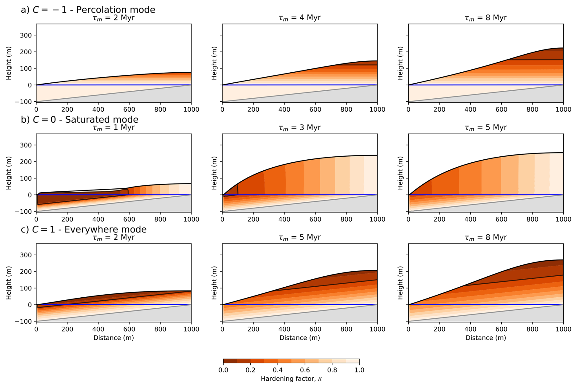
Figure 22 Model experiments in which we varied the mass loss time scale τ_m while keeping all other parameter constant, including the laterisation time scale τ_l at a value of 8 Myr. As indicated, each row of experiments corresponds to a different mode while each column to different values of τ_m.

As already pointed out above, in the percolation mode, the mass loss time scale mostly controls the thickness of the predicted duricrust but does not affect much its position or the geometry of the regolith layer. However, in the saturated and everywhere modes (middle and bottom rows of experiments in Fig. 22), varying τ_m affects strongly the geometry of the duricrust as well as its thickness.

In the saturated mode, for small values of τ_m, mass loss can be so efficient that it causes the duricrust to be progressively buried by sediments deposited on top of it. In this case, the duricrust forms parallel to the weathering front and thus oblique to the water table or surface topography. For values of τ_m larger than τ_l, no duricrust forms.

This surface sedimentation is an autogenic process, i.e., that accompanies the laterisation of the regolith independently of external forcings, such as a drop in base level. Interestingly, it predicts an age distribution with depth with a maximum in both primary and secondary weathering ages (Fig. 23) at the depth of the buried duricrust layer. This is very similar to recent observations made in a profile near Manaus in the Central Amazon Basin (Brazil) (see Fig. 15 in Ansart et al., 2025). These authors interpret the ages as a function of external, mostly climatic signals (Fig. 16 in Ansart et al., 2025). Our model results show that such a distribution can be the result, in parts or in whole, of mass loss-driven surface sedimentation.

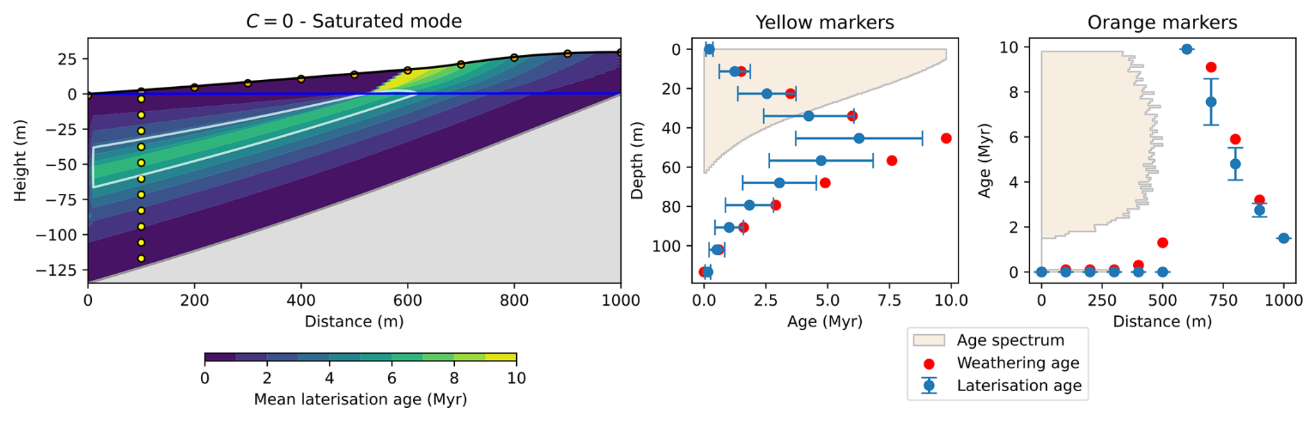
Figure 23 Contours of secondary weathering ages (left panels) for an experiment in the saturated mode and a mass loss time scale (τ_m = 2 Myr) smaller than the laterisation time scale (τ_l = 5 Myr). Uplift rate is set to 20 m Myr⁻¹ to enhance the effect of duricrust burial by sedimentation. Age distributions along a vertical profile and the surface of the model are shown in the central and right panels.

In the everywhere mode, decreasing τ_m leads to the duricrust forming closer to the base level, while increasing it causes the duricrust to form closer to the hill top.

5.4 Climate variations and duricrust formation

It is commonly accepted to relate the formation of weathering products, including hardened layers, to past climatic conditions (Vasconcelos et al., 1994; Ruffet et al., 1996; Hénocque et al., 1998; Allard et al., 2018; Heller et al., 2022; Ansart et al., 2022, 2025). Clustering in age distributions within a regolith profile, whether they relate to the timing of secondary weathering or to the formation of hardened layers, are often interpreted in terms of global or local climatic events (e.g. Ansart et al., 2025). Our model seems to support this approach with predicted age clustering that are strongly correlated to periods of enhanced precipitation (Fig. 18). This, however, is a direct consequence of our parametrization that assumed that the effective rate of laterisation depends linearly on precipitation rate (Eq. 5). More interestingly, our model also predicts no age clustering associated with periods of enhanced or reduced rate of base level lowering (Fig. 17). This implies that climate signals stored in age distributions should be more easily identified than tectonic signals.

Moreover, the model predicts that during climatic cycles, periods of enhanced precipitation always result in an enhancement of the chemical erosion flux, with respect to the physical erosion flux (Fig. 21). This is directly related to our assumption of a linear relationship between secondary weathering rate and precipitation, but also to the reduced physical erosion efficiency resulting from the surface lowering associated with enhanced chemical erosion during wet periods. Of course, enhanced precipitation can also directly affect the efficiency of physical erosion through enhanced surface runoff that promotes hillslope transport by overland flow or denser vegetation that reduces transport by soil creep. Richardson et al. (2019) suggest that there may exist a precipitation threshold below which the transport coefficient increases with precipitation rate and above which this trend is inverted. This complexity in determining a simple relationship between climate (precipitation) and physical erosion (by surface transport) led us to neglect this process in the model. It would be very interesting, however, to investigate the effect of such a feedback.

5.5 Comparison of WTF and LAT models

Duricrust formation conditions remain an active area of research. Nonetheless, there is consensus on two primary hypotheses for duricrust formation (Goudie, 1985; Bourman, 1985). These hypotheses apply to different types of duricrusts, yet distinguishing between them and determining their formation processes can be challenging. To address this, we have developed models representing both hypotheses, one for the absolute accumulation or transport (WTF) model, as presented in Fenske et al. (2025) and the second for the relative accumulation or in situ model (LAT) as presented in this study. A key question now is whether the results from these models can help us effectively differentiate between the two hypotheses and elucidate the conditions under which each type of duricrust forms.

There are two main controls on duricrust formation in the WTF model: tectonic quiescence and water table fluctuations (WTF). A period of total or near-total tectonic quiescence is essential for duricrust formation, given the critical importance of proximity to the water table fluctuation range. Uplift (or base level drop) plays an important role in exhuming a duricrust and bringing it near or at the top of a hill to form a capped plateau (Fenske et al., 2025). The thickness of the duricrust itself is primarily determined by the extent of the water table fluctuation range represented by λ in the WTF model. Seasonal water table fluctuation ranges are relatively well constrained (see compilation in Fenske et al., 2025). The thickest observed duricrusts are found in environments with significant contrast between dry and wet season water table heights. Thickness does not exceed a few metres to tens of metres. No steady-state situation can be achieved using the WTF model.

We showed in this study that, in contrast to the WTF model, material in the LAT model needs to be continuously advected from the bedrock to the regolith for a duricrust to form. Therefore, some but slow tectonic activity (or base level drop) is required for duricrust formation. As long as material supply continues, a duricrust can develop indefinitely. Its thickness is determined by material supply, mass loss rate and erosion. In contrast to the WTF model, a steady-state can potentially be reached when surface subsidence caused by mass loss perfectly balances uplift. In this situation a duricrust can form and progressively grow either at the surface or within the regolith layer, depending on the mode (percolation or saturated) that is activated. However, as soon as the duricrust is exposed to the surface, it will slow down the erosional efficiency, which, in turn can cause the duricrust to continuously thicken and will prevent the system to reach steady-state.

Both models can also be used to predict hardening age distributions as well as primary weathering ages. Age distributions within a weathering profile can help determine which of the two formation mechanisms (WTF or LAT) is the most appropriate. Indeed, comparing the ages predicted by the two models, two main aspects can be considered. The first concerns the relationship between the age of the duricrust and that of the surrounding regolith. If older regolith is observed above the duricrust, then this configuration is more consistent with duricrust formation by WTF (as shown in Fig. 2a). WTF duricrusts typically form in the subsurface, along the water table fluctuation range (Fenske et al., 2025), thus the regolith below and above is unaffected by duricrust formation and evolves independently provided there is no shift in base level. This reasoning has a similar approach to the cross cutting principle where features that form or cut through an already existing layer is younger than the layer itself. Conversely, if the duricrust is older than the overlying regolith, it implies that the regolith may consist of transported soils deposited on the duricrust, which formed by LAT (Fig. 2b). However, it should be noted that removal of the overlying regolith by erosion might change the age profile of the column, potentially making it more difficult to differentiate between the two models. In situations where there is no regolith above the duricrust or where erosion reworked the material, age distributions can provide clues. An asymmetrically broadening aging age distribution from the lower layers to the surface of the weathering profile indicates formation by LAT, as it is typically found in nature for comparable weathering profiles (Shuster et al., 2012). In contrast, duricrusts formed by WTF may exhibit age distributions that reflect characteristics of external sources, lacking any trends. Additionally, if there are multiple generations of duricrusts present in a single hill, it is most likely indicative of WTF formation. In contrast, duricrusts formed by LAT tend to develop as a single continuous entity from the underlying weathering profile.

These general considerations regarding the use of the two models to help determine, in a given situation, which of the two duricrust forming hypotheses is most applicable, have limits. In Fig. 24, we show the results of three separate experiments in which we assumed that the formation of duricrusts is governed by the LAT model in the percolation mode (Fig. 24a), the LAT model in the saturated mode (Fig. 24b) and the WTF model (Fig. 24c). In all three experiments, we assumed the same tectonic uplift scenario made of two episodes of rapid uplift (U = 100 m Myr⁻¹) of 10 Myr duration each, and each followed by a 10 Myr long period of tectonic quiescence (U = 0 m Myr⁻¹). All other model parameters and the initial geometry are identical, except for the laterisation and mass loss time scales that are set at τ_l = τ_m = 5 Myr in the LAT/percolation experiment, and at 10 Myr in the LAT/saturated experiment, while the hardening time scale, τ, is set at 2 Myr in the WTF experiment. Results from the three experiments are shown in Fig. 24 as snapshots of the model evolution at the end of each phase, i.e., at 10, 20, 30 and 40 Myr, as well as contour plots of the predicted regolith and hardening ages.

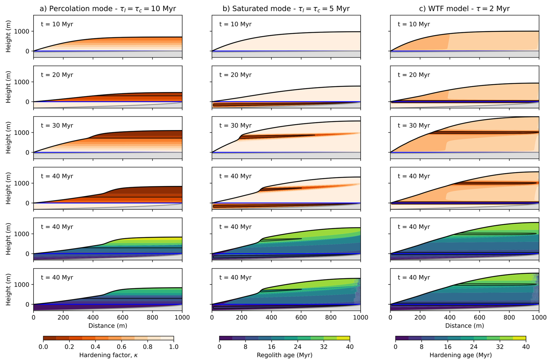
Figure 24 Comparison between three model experiments using (a) the LAT model in the percolation mode, (b) the LAT model in the saturated mode and (c) the WTF model. In each column, the top 4 panels show the time evolution of the distribution of the hardening parameter, κ. The bottom two show the predicted regolith and hardening ages. The black line corresponds to the κ = κ_c contour. All model parameters are identical in the three experiments, including the uplift function made of two episodes of active uplift (U = 100 m Myr⁻¹) of 10 Myr duration each followed by a period of tectonic quiescence. τ_l = τ_m = 10 Myr in the LAT/percolation experiment and τ_l = τ_m = 5 Myr in the LAT/saturated experiment and τ = 2 Myr in the WTF experiment.

We see that all three models predict the formation of one or two duricrusts. The LAT/percolation model's duricrust is very thick and forms continuously during the experiment, but preferentially during the quiet phases. In the two other cases (LAT/saturated and WTF models), the model predicts the formation of two duricrusts, that formed exclusively during the quiescence periods, either below the water table (LAT/saturated case) or within the water table fluctuating range (WTF case). The thickness is set by the duration of the quiet period (with respect to the laterisation time scale) in the LAT/saturated case and by λ, which we set to 5 m, in the WTF case. Both regolith and hardening age distributions look very similar in all three cases, except for the vertical offset between the regolith and hardening ages in the LAT/percolation case, which corresponds to the time spent by rock particles in the regolith beneath the water table. In the LAT/saturated case, the duricrusts experience downward displacement in the regolith column due to the mass loss associated with duricrust formation. Despite this, sedimentation does not occur due to the large topography that is created during the uplift phases.

To differentiate between the possible formation mechanisms, and especially between the LAT/saturated and WTF hypotheses, the geometry, thickness, position of the duricrust and their age relative to that of the surrounding regolith do not provide sufficient information. Detailed geochemical analysis, and, in particular, the isotopic composition of the bedrock, regolith and duricrusts remain the most likely method to distinguish between the plausible scenarios. Isotopic data are particularly revealing as duricrusts formed by hydrological processes do not present any genetic link to the regolith and bedrock below, as they formed from an external input of material (Ollier and Galloway, 1990; Taylor and Eggleton, 2001). In contrast, duricrusts formed by laterisation are derived from in situ bedrock weathering, and the two are therefore genetically linked (Tardy and Roquin, 1992). By investigating the isotopic compositions across the profile, it is possible to assess whether a genetic link between the regolith and duricrusts exists, thus identifying which mechanism was at play.

5.6 Combining the two models

Recently, detailed geochemical and geochronological studies of weathering profiles from stable cratons (Goudie, 1985; Ansart et al., 2025) have shown that hardened layers of different origin (i.e., that formed either by LAT or WTF) can coexist in a single regolith layer. They are likely to be the product of distinct episodes of laterisation/hardening.

In Fig. 25 we present age predictions of a model experiment where the two models of duricrust formation have been combined. To understand the evolution of this model, we also show snapshots of contour of the predicted hardening parameter, κ, in Fig. S19. The model experiment lasts 10 Myr and includes a period of slow uplift (U = 30 m Myr⁻¹) of 5 Myr duration, followed by a quiescence period. We combined the LAT/saturated model with τ_l = τ_m = 5 Myr and the WTF model with τ = 1 Myr and λ = 5 m. The combined hardening parameter is the product of the hardening parameter predicted by each model.

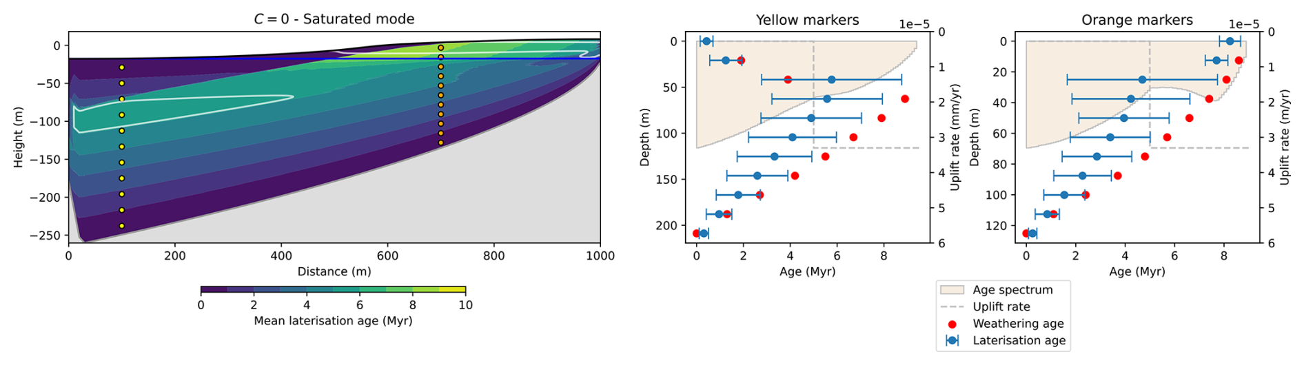
Figure 25 Predicted ages in a model experiment combining the LAT and WTF models. Areas within the white contours correspond to duricrusts (κ < κ_c).

Two duricrusts have formed, both mostly during the quiet episode. Interestingly, the upper duricrust is older than the lower one and its hardening age is significantly older than the regolith on which it sits. In contrast, no such discontinuity in duricrust age between the buried duricrust and the underlying regolith is predicted, but sediments on top of the LAT duricrust have ages that progressively young towards the surface. At the end of the model experiment, the duricrust formed by WTF caps the hill, the other, formed by LAT, is buried beneath several tens of metres of material. The overlying sediments were deposited from higher elevations, i.e. the top of the hill, during the evolution of the topography and formation of the duricrust.

The results of the experiments shown in Fig. 25 demonstrate the complexity of situations that can be produced in a relatively simple tectonic setting when combining the two models while using different characteristic time scales for hardening. It is beyond the scope of the work presented here to report the many different situations that can arise by varying combined model parameters. This example shows how the model can be used to explain apparently complex duricrust geometries and age distributions, without the need for complex tectonic or climatic scenarios.

6 Conclusions

We have developed a new model for the formation of duricrusts by laterisation (i.e. the in situ model) by modifying an existing model for the formation of regolith by chemical weathering (Braun et al., 2016). In this model, hardening is caused by progressive leaching of the most soluble minerals from the regolith layer, leading to concentration of insoluble minerals and species, and their ultimate amalgamation into erosion resistant layers, i.e., the duricrusts. The model assumed that laterisation and the ensuing hardening of the regolith is a self-limiting process that is linearly proportional to precipitation rate and is accompanied by mass removal. In the model, this leads to volume change within the regolith, and to surface subsidence. We implemented three laterisation modes, including the percolation mode where laterisation and hardening are limited to the part of the regolith that is above the water table, the saturated mode where laterisation is limited to areas below the water table and the everywhere mode where laterisation takes place everywhere.

We have shown a large number of model experiments varying both the model internal parameters (the various time scales and the mode) and external forcings (uplift and precipitation rate). Using insight from these experiments, we have derived a simple condition for the development of a duricrust under constant forcing. We have shown that duricrust formation is most likely in regions of low uplift and high precipitation rate.

The model also illustrates the importance of considering mass loss associated with laterisation. This can result in steady-state situations in the percolation mode where surface uplift is balanced by erosion and surface subsidence due to contraction, and to the progressive burial of a duricrust forming in the saturated mode.

We have also shown how age distributions can be extracted from the model results. We have subsequently shown how each mode leads to characteristic age distributions and how various episodes of enhanced precipitation or reduced uplift rate affect the distribution of ages in a regolith profile.

We have also shown how the model can be used to predict the relative proportion of chemical vs. physical erosion and how this ratio varies during successive episodes of uplift activity or in under varying precipitation scenarios.

We have finally shown how, by comparing the new model results with those obtained by assuming that duricrust formation is the result of water table fluctuations (the WTF model previously developed and presented in Fenske et al., 2025), one can, potentially, use the geometry, position and age of a given duricrust to estimate which of the two competing mechanisms is responsible for its formation.

Due to its efficiency, the model can be used to perform ensembles of simulations to explore model parameter values that can explain observations at a given site. This is what we intend to do in the future in view of the increasing number of studies where the necessary data (ages, geochemical data, etc.) is available (Théveniaut and Freyssinet, 1999; Vasconcelos and Carmo, 2018; Allard et al., 2018; Heller et al., 2022; Lipar et al., 2024; Ansart et al., 2025, for example).

We are also currently working on a three-dimensional version of both duricrust formation models that we intend to incorporate into a landscape evolution model to better study the complex interactions and potential feedbacks between regolith formation, tectonics, climate and surface processes.