OrthoSAM: multi-scale extension of the Segment Anything Model for river pebble delineation from large orthophotos

Sediment characteristics and grain-size distribution are crucial for understanding natural hazards, hydrologic conditions, and ecosystems. However, traditional methods for collecting this information are costly, labor-intensive, and time-consuming. To address this, we present OrthoSAM, a workflow leveraging the Segment Anything Model (SAM) for automated delineation of densely packed pebbles in high-resolution orthomosaics. Our framework consists of a tiling scheme, improved seed (input) point generation, and a multi-scale resampling scheme. Validation using synthetic images shows high precision close to 1, a recall above 0.9, with a mean IoU above 0.9. Using a large synthetic dataset, the two-sample Kolmogorov-Smirnov test confirms that there is no significant difference between the predicted and the ground-truth grain size distributions. We identified a size detection limit of 30 pixels; pebbles with a diameter below this limit are not reliably detected. Applying OrthoSAM to orthomosaics from the Ravi River in India, we delineated 6087 pebbles with high precision (0.93) and recall (0.94), based on manual verification of each predicted mask. The resulting grain statistics include area, axis lengths, perimeter, RGB statistics, and smoothness measurements, providing valuable insights for further analysis in geomorphology and ecosystem studies.

1 Introduction

In Earth sciences, grain size analysis is a crucial technique used to study the physical characteristics of sediments, soils, and rocks (e.g., Parker, 1991; Rice et al., 2001; Rice and Church, 1998). The primary aim of grain-size analysis is to determine the distribution of particle sizes within a sample or for a specific area in the field, which can provide valuable information about the sediment's origin, transport history, and depositional environment.

Traditional approaches such as the “Wolman Pebble Count” (Wolman, 1954; Leopold, 1970) require that a trained observer with a metric ruler record the sizes of the pebbles along streams. Pebble counts can be made using grids, transects, or random step-toe procedures to provide statistical averages of grain sizes. While this approach is precise and accurate, it is time-consuming and usually does not provide a large number of grain-size measurements. But counts of more than a few hundred pebbles are required to successfully delineate grain-size distributions and link geomorphic processes (e.g., Purinton and Bookhagen, 2021; Eaton et al., 2019; Sklar, 2024).

The advancement of digital photography and 3D structural data over the past 20 years has enabled the development of alternative pebble-counting methods. We collectively refer to these methods as photo-sieving approaches without specifying a methodological approach, but with a common goal to derive grain-size distributions. Methods to estimate grain-size distributions are diverse and range from lag autocorrelation analysis (Rubin, 2004), two-dimensional spectral decomposition (Buscombe et al., 2010), image-roughness estimations (Carbonneau et al., 2005), deterministic algorithms to extract individual grains and measure diameter or a- and b-axes of pebbles (Purinton and Bookhagen, 2019; Carbonneau et al., 2018), machine-learning approaches to estimate distributions directly (Buscombe, 2020) or perform grain segmentation (Mair et al., 2022), and delineate pebbles from 3D mesh or point-cloud data (Steer et al., 2022; Rheinwalt et al., 2025). Radar-based studies have attempted to use the scattering signal of C- and L-band data (e.g., Purinton and Bookhagen, 2020). Satellite or airborne images often rely on image texture and semi-variance or related properties and field calibration to derive the grain-size distribution without counting individual pebbles (Carbonneau et al., 2004; Butler et al., 2001; Ibbeken and Schleyer, 1986). Recent advances in UAV-based data acquisition allow the generation of higher-resolution imagery that can be used for individual pebble segmentation, although there is a limit on the smallest pebble sizes due to image resolution (Lang et al., 2021; Purinton and Bookhagen, 2019). Part of the attraction to using remote-sensing approaches is to achieve observations at scales ranging from the meter (often referred to as patches) to the kilometer scale (entire drainage basins). In addition, it is also possible to sample a larger number of grains and include a larger range of grain sizes. A new motivation is to extract pebble roughness or roundness metrics, such as the isoperimetric parameter (e.g., Pokhrel et al., 2024; Quick et al., 2019).

Object delineation in material and biological sciences has long been applied and has been fine-tuned to specific approaches. One of the most widely used convolutional neural network approaches for image segmentation, U-Net, has been motivated by biomedical research and was initially developed for cell delineation (Ronneberger et al., 2015). Other deep-learning research has focused on the detection of tree crowns (e.g., Chen et al., 2025; Weinstein et al., 2020). Although these approaches are creative and highly optimized, they are not directly applicable to pebble counting in fluvial environments. First, the grain size distribution of a mountain river is large, with the smallest sizes in the (sub-)mm range to meter-sized boulders. This large size range requires different approaches to counting similarly sized spherical objects. Second, fluvial pebbles have a variety of shapes and colors that complicate detection. The changing shadows and lighting conditions make this particularly challenging for a deterministic approach (Cattapan et al., 2024; Purinton and Bookhagen, 2019).

Despite or because of these challenges, deep-learning approaches have become increasingly popular in the delineation of pebbles from imagery (e.g., Mortl et al., 2022; Mair et al., 2024; Soloy et al., 2020). They provide the ability to automate measurements, improve reproducibility and scalability, and increase the number of observations. Deep learning can overcome some of the limitations of traditional methods for measuring grain size, especially when considering processing speed and delineating images with high complexity. The drawback of using deep-learning approaches is that they require large, high-quality training data. Deep-learning models can overfit the training data, and their results can be difficult to interpret. The measurement of small grains can be challenging for deep learning methods. The scale and resolution of input images to some deep-learning models can be limited by GPU memory and model complexity, and deep-learning models generally require higher computing resources. One of the likely more relevant drawbacks is that current segmentation techniques are prone to biases that result from under- or over-segmentation and 2D projection effects of 3D structures.

In a previous effort, the Segmenteverygrain project (Sylvester et al., 2025) leverages the Segment Anything Model (SAM; Kirillov et al., 2023) to delineate grains in images. This approach adopts a two-pass pipeline combining a pre-trained U-Net with SAM. In the first pass, a U-Net model performs semantic segmentation to distinguish grains from non-grain objects. In the second pass, SAM is applied to perform instance segmentation only on the grains identified in the previous step. This approach benefits from effectively filtering out irrelevant objects, but it introduces dependency on the U-Net.

A successful workflow for an application of a deep-learning approach in sedimentary research requires model adoptions, for example, a tiling approach that allows the input of large orthomosaics and a statistical analysis of a model's output to assess uncertainties of the segmented image. In this study, we explore the capabilities of the SAM for pebble segmentation, describe the model in detail with its benefits and caveats, and develop a workflow that allows the delineation of complex images with a specific focus on fluvial pebbles through a tiling scheme, an improved input point generation, and a multi-scale resampling scheme. We use a synthetic pebble image as input to SAM to first identify minimum and maximum object sizes and perform statistical analysis with a large number of pebbles. In the second step, we apply SAM to three characteristic field examples from the Ravi River in the western Himalaya.

2 The Segment Anything Model (SAM)

The Segment Anything Model is an efficient and adaptable foundation model for image segmentation. It was trained with over 1 billion masks in 11 million licensed and privacy-respecting images and generates excellent segmentation results without additional training (Kirillov et al., 2023). SAM enables segmentation of a broad set of use cases and can be used out of the box on new image domains without additional training, including scientific images such as cell microscopy or pebble images (Na et al., 2024; Israel et al., 2023). Our analysis relies on SAM v1 (Kirillov et al., 2023). The more recent SAM v2 (Ravi et al., 2024) was not tested, since its advancements are focused mainly on video segmentation and tracking, which are outside the scope of our analysis.

SAM has the ability to segment images with complex lighting conditions and conglomeratic boulders. This stems from SAM's very good zero-shot inference. SAM can accurately segment images without prior specific training, a task that traditionally requires tailored models. The model's architecture consists of three decoupled components: an image encoder, a prompt encoder, and a mask decoder, which provide an efficient framework for performing multiple tasks on an encoded image through multiple inputs such as user queries, points, polygons, or text input.

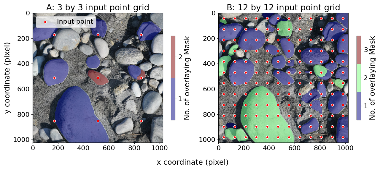
Figure 1 SamAutomaticMaskGenerator segmentation result of a 3 × 3 (A) and 12 × 12 (B) point grid. The segmentation was performed with the default parameters. The number of input points determines the number of objects that can be segmented. SamAutomaticMaskGenerator includes several post-processing steps to remove duplicated masks. With the use of more input points, there is a higher likelihood of generating under-segmentation (masking multiple objects) or over-segmentation (masking only part of an object). These masks cannot be easily removed by the built-in post-processing steps, as they are not simple duplications. However, with too few input points, many pebbles are missed and not segmented at all.

However, SAM has limitations when it comes to detecting densely packed objects such as pebbles or sand in high-resolution images. The input data for the delineation of the pebbles are usually large orthomosaics generated from hand-held cameras (e.g., Purinton and Bookhagen, 2021) or UAV images (Mair et al., 2022). SAM rescales all input images to 1024 × 1024 pixels to fit the transformer architecture – a large image with several thousand pixels in width and length will be rescaled when processed by SAM. The prompt encoder requires input points to identify objects. Input points can be thought of as a coarser raster draped over the input image to identify points of interest: The finer the scale of this raster, the more grains can be detected (Fig. 1). The standard SAM model applies 32 × 32 equally spaced input points in the standard, automated detection scheme. The transformer and prompt encoder were optimized for a limited number of objects, not hundreds to thousands of objects per image, as would be the case for pebbles on a large orthomosaic. The performance of the model is further limited by hardware resources, and it may require strategies such as tiling, resampling, or manual input to detect all objects in an image (Fig. A1). Despite these limitations, SAM has the potential to be a powerful tool for image segmentation in various fields, including geology and environmental science. Additional details and background information about SAM can be found in Appendix A.

3 Data

We validate our approach with two different datasets: (1) a synthetic pebble generator with a variety of noise and shadowing settings; (2) a manually labeled dataset of an orthomosaic for a complex pebble setting derived from the Ravi River in northwest India in the western Himalaya. Validation through real-world orthomosaics is limited because it requires large ground-truth data. We are not aware of reliable, large-scale instance segmentation datasets with several hundred to thousands of delineated pebbles. Hence, we put forward a synthetic pebble-generation approach for quantitative, rigorous testing, and the semi-manually labeled Ravi River data for a proof-of-concept application.

3.1 Validation with Synthetic Images

Synthetic scenes were generated at a resolution of 10 000 × 10 000 pixels with solid circles of random sizes placed randomly. The placement process ensured that the circles did not overlap, with at least one pixel distance between them. This process was repeated 5000 times to create up to 5000 circles per image (Fig. 2).

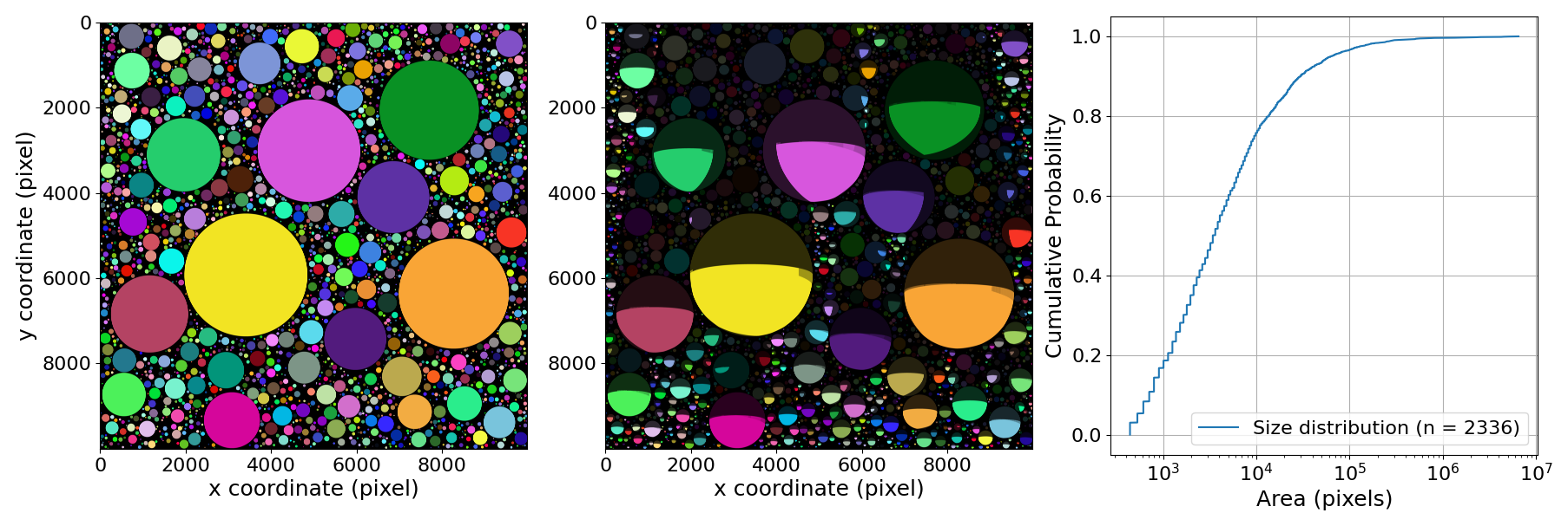
Figure 2 Example of a noise-free, shadowed, and colored synthetic test scene with n = 2336 pebbles. The parameters for generating this scene are: r_min = 12; r_max = 1500; σ = 0. The size distribution of the pebbles is shown on the right and is highly skewed.

Synthetic images were generated in four settings: black and white (B&W), colored, colored with noise, and colored with shadows (colored images have random colors). Noise was introduced to colored images using Gaussian noise with a controlled standard deviation ranging from 3 to 192 for each 8-bit channel. This allowed for the assessment of SAM's performance on various image types and its robustness against noise. The parameters used to generate the synthetic scenes are listed in Table A1. Additional information on the synthetic pebble generation is found in Appendix B.

To simulate a more realistic setting, we have further introduced shadows into the synthetic images. Each circular object is modeled as a hemispherical dome, and shadows are simulated based on geometric occlusion. Specifically, cross-shadowing is implemented, allowing shadows from one object to be cast onto others, under the assumption of a directional light source at infinity. This ensures a uniform lighting direction across the entire scene. To reduce computational complexity, diffusion, diffraction, and reflection effects are not modeled. Instead, shadows are applied as uniform attenuation, with adjustable strength to approximate soft shadowing behavior.

3.2 Ravi Orthomosaics

Three characteristic examples from the western Himalaya (Ravi River) in India are used to illustrate the workflow (Fig. 3). The orthomosaics were scaled with 24 markers on four A4 panels. The photos were processed with Agisoft Metashape 2.1.2. For model Ravi2, we used 467 photos, Ravi3 is based on 708 photos, and Ravi4 on 716 photos. We used a Sony 7RM3A with a fixed 55 mm lens (F1.8) with 41 MP (7952 × 5304 pixels). The orthomosaics have a spatial resolution of 0.2 mm.

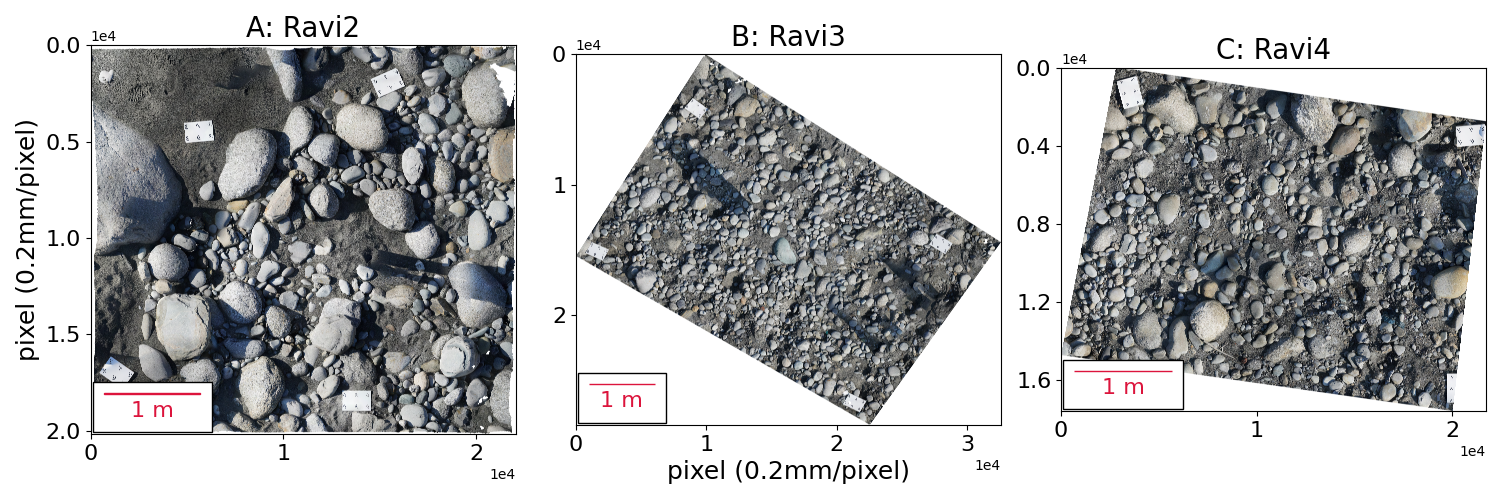
Figure 3 Three orthomosaics from the Ravi River, western Himalaya: (A) Ravi2 (20 171 × 22 055 pixels); (B) Ravi3 (28 382 × 32 563 pixels); (C) Ravi4 (17 592 × 21 739 pixels). All three images have a resolution of 0.2 mm per pixel.

In order to generate the manual validation dataset, we also used a digital elevation model with 0.5 mm resolution generated from the 3D point cloud. The DEM was subsampled to match the orthomosaic resolution. We used the DEM hillshade to assist in manual checking and visualization of validation points.

4 Methodology: OrthoSAM

Our tiling and resampling scheme, referred to as OrthoSAM, consists of three main components: tiling, the generation of improved input points, and resolution passes (Fig. 4). Additional details can be found in Appendices C to E, and the parameters used to segment the Ravi orthomosaics are listed in Table A2.

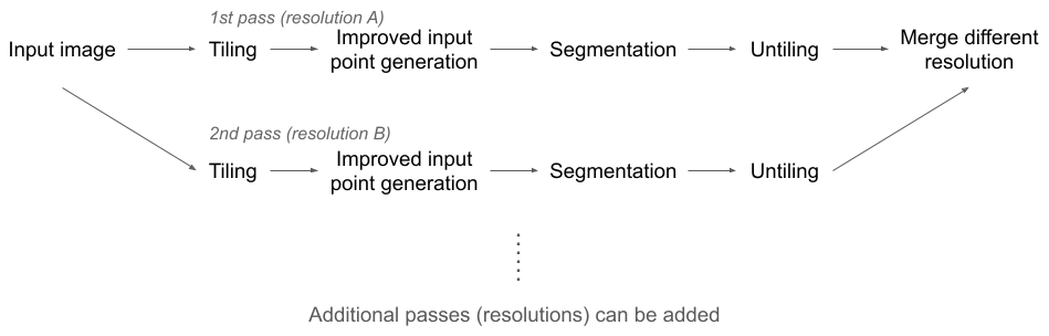
Figure 4 Flow diagram of the OrthoSAM approach. We rely on multiple resolutions of the input image to segment pebbles at various scales. In theory, multiple resolutions can be used and merged – but here we only show two resolutions (A and B). A complete segmentation of the entire image at a given resolution is referred to as a pass. Segments from earlier passes take priority over those from later passes during the merging process. We usually use the original resolution as the first step, as resampling to a coarser resolution inherently leads to information loss. In most cases, a fine, initial resolution is followed by a coarser resolution to process objects that are too large to fit within a single tile with a finer resolution.

4.1 Tiling of Input Image

The SAM model rescales and pads the input images to 1024 × 1024 pixels, which can lead to a loss of information for larger images. For example, a 24 MP image (6000 × 4000 pixels) would be reduced to approximately 0.7 MP, which may not be sufficient for segmenting small objects like pebbles in large orthomosaics. After rescaling, small objects may be overlooked, or larger objects may have reduced mask quality (Fig. 5). To address this, a tiling approach is necessary for large images with many objects.

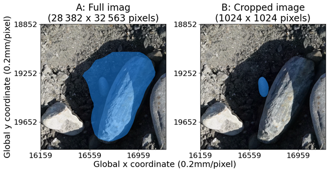
Figure 5 Comparison of segmentation quality. (A) The full-resolution image of 28 382 × 32 563 pixels was provided to the encoder, and the encoder downscales the image to 1024 × 1024; (B) a 1024 × 1024 crop around the target was provided to the encoder. Both images have the same resolution, but image A was rescaled by SAM. Segmentation was performed with identical input points and parameters using the standard SAM approach. Results differ because of the encoder resampling.

To process large images, we tile them into 1024 × 1024 pixel patches with a definable overlap. This helps reduce the likelihood of overlooking objects, but can also lead to artificially over-segmented pebbles along tile edges. To mitigate this, we discard masks that touch the window border and use a rectangle box to filter out masks that do not meet the criterion of having at least 50 % of masked pixels inside the box. The processed patches are then combined into a 2D-labeled mask (see Appendix C).

4.2 Improved Input Point Generation and Segmentation

SAM can deliver high-quality results, but is not ideal for delineating pebbles from large orthomosaics. To improve this, we developed an approach that generates input points more effectively. Our method involves an initial pass to extract all possible objects using a modified version of the SamAutomaticMaskGenerator (see Appendix D). We use a parameter n_pps to define the number of input points per side, in order to maximize the probability that every object will get at least one input point. The trade-off is an increase in computational cost and processing time. We also consider the minor-axis length of the smallest object expected and adjust to define the number of input points per side. If hardware limits are reached, we can increase tile overlap or resample the image to a finer resolution to increase the input point density. Once the point grid is generated, each point serves as an input prompt for the SAM, which generates three mask predictions (see Appendix C and Fig. A1). We select the mask with the highest predicted Intersection over Union (IoU) score as the final output, after a centroid-based masking step (see Appendix D and Fig. A2).

4.3 Merging Segmentation Passes at Multiple Resolutions

The SAM approach has a limitation that the detectable size is artificially capped due to the window size and maximum window coverage. To address this, segmentation can be performed at multiple resolutions, with each resolution corresponding to objects up to a certain size. The final results can be merged to ensure that objects of all sizes are delineated (Fig. 6).

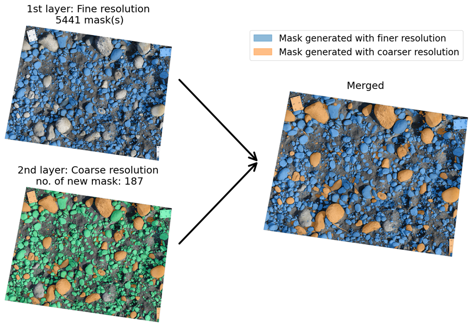
Figure 6 Characteristic example showing the merging of two different resolutions. The original image has 28 382 × 32 563 pixels with a resolution of 0.2 mm per pixel. The first, fine-resolution segmentation, identified 5441 masks. The coarser resolution (1135 × 1303 pixels), downsampled by a factor of 25, results in 187 masks. The coarser masks only segment larger pebbles and include the boulders that are excluded in the first step because they cover more than 40 % of the tile. The proposed and described merging step uses all masks from the fine resolution (first step) and adds masks from the second step in the remaining space. The resulting merged image highlights the masks from the first step in blue and the second step in orange.

The merging process involves identifying areas where no mask was found in the first resolution pass and comparing them with masks from the second resolution pass (see Appendix D). Masks are only merged into the final result if they do not overlap with masks from the first resolution. This approach can be used with any resolution order, with the order setting the priority in the merging process.

Using multiple resolution passes can help reduce aliasing effects and preserve segmentation quality for larger objects. A fine-coarse combination can reduce the reduction of mask quality due to aliasing, while a coarse-fine combination can minimize over-segmentation. Additional intermediate resolution passes can be introduced to handle images with a wide range of object sizes, although this increases processing time (Appendix E).

4.4 Validating OrthoSAM

We evaluate the segmentation of synthetic pebble images in three aspects. First, we assess detection quality, which refers to whether OrthoSAM identifies all objects and whether the detected objects are true objects. Second, we examine the mask quality by how accurately objects are segmented. Finally, we analyze the measured size distribution to determine whether it accurately preserves the true size distribution.

We evaluate the detection quality by matching masks to labels based on their centroids. A mask is assigned to the label on which its centroid falls. When a mask is paired to a label that has not yet been paired with any other mask, it is counted as a true positive (TP). If a mask is assigned to a label that has already been matched with another mask, it is considered a false positive (FP). If a mask does not match any label, it is also counted as a false positive. Since these are synthetic images, the total number of actual positives (the label count n_l) is known. Using the true positives, the number of false negatives (FN) can be determined. With TP, FP, and FN values, precision, recall, and Average Precision (AP) can be calculated to assess overall detection quality. Due to the lack of confidence values in Segment Anything output, we modified the calculation of AP to use object size as a proxy for confidence.

We use two sets of synthetic models: A black-and-white (B&W) setting to evaluate the size detection limit and a colored model with shadows to illustrate varying lighting conditions (see Appendix B). A total of 48 synthetic images with varying parameters were generated and segmented (see Table A2).

5 Results

In this section, we first present the segmentation statistics of the synthetic pebble images and analyze the limitations of OrthoSAM. In a second step, we present statistics for real-world scenarios.

5.1 Synthetic Pebble Images and Segmentation Statistics

Using 1872 synthetic B&W pebbles, we obtain an overall recall of 0.87, a precision of 1.0, an AP@0.75 of 1.00, and a mean IoU of 0.98. Using 27 528 synthetic colored pebbles with shadows, OrthoSAM segmentation achieved a recall of 0.94, a precision of 0.98, an AP@0.75 of 0.87, and a mean IoU of 0.91 (Tables A3 and A4).

To analyze the limits of OrthoSAM, our approach was two-fold: We used B&W synthetic pebble models to identify a size threshold. Second, we used colored models with shadows to illustrate the impact of changing lighting conditions.

Precision and recall metrics are used to evaluate object detection, and IoU is used to evaluate the mask quality and the accuracy of the segmentation. We observed that a recall above 0.9 is only achieved for pebble diameters greater than 30 pixels (Fig. 7). Whereas a consistently high IoU above 0.9 is only achieved for pebble diameters greater than 20 pixels (Fig. 8). To ensure that an object is both detected and well-segmented, we identify the size detection limit at 30 pixels. We only used the B&W pebbles for measuring the detection limit because we wanted to exclude obscuring conditions such as color variability or shadowing.

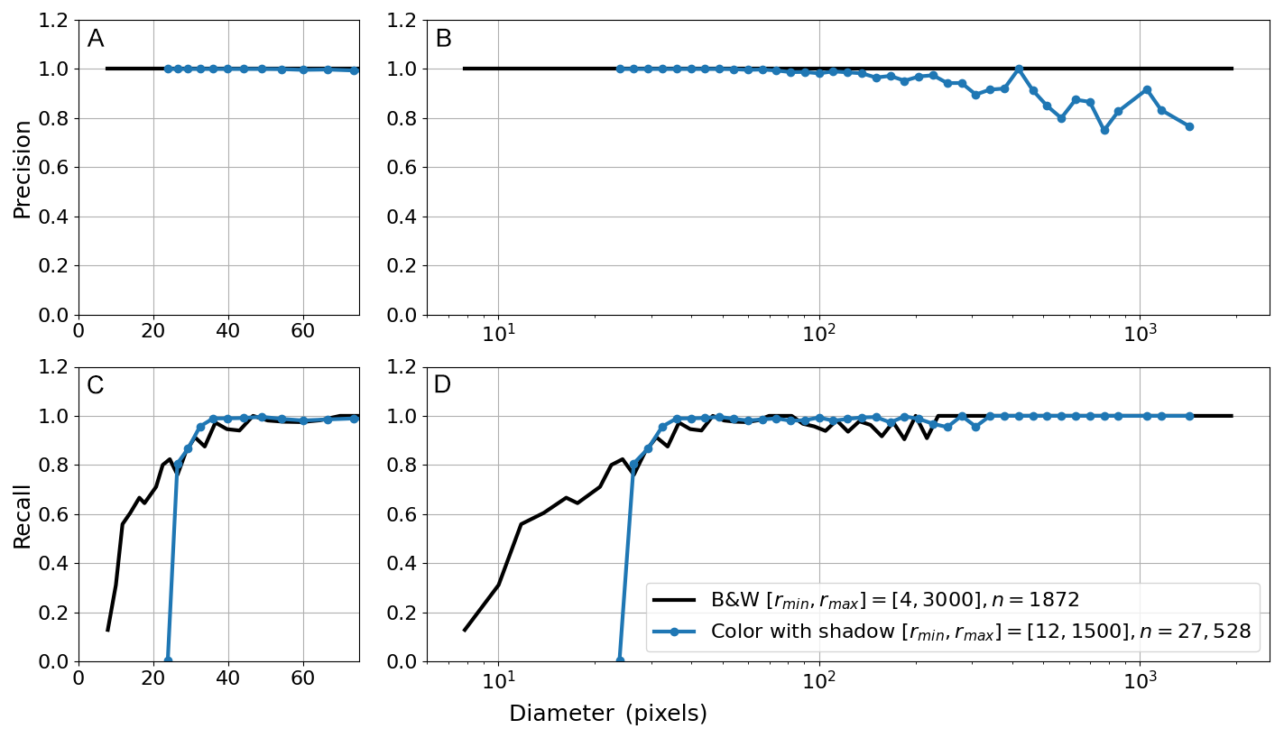
Figure 7 Binned precision and recall of the B&W synthetic scene (n = 1872 pebbles) without shadows and the colored synthetic scene (n = 27 528 pebbles) with shadowing. Labels are grouped by diameter into logarithmic bins to compute precision and recall within each bin. Precision (A) and recall (C) of objects with a diameter below 75 pixels to highlight the size-detection limit. Recall drops below 0.9 for diameters less than 30 pixels. Precision (B) and recall (D) for the entire size range of synthetic pebbles show an overall high level of precision. The precision variability at higher diameters is discussed in the text and is related to pebbles partly in shadow at tile boundaries.

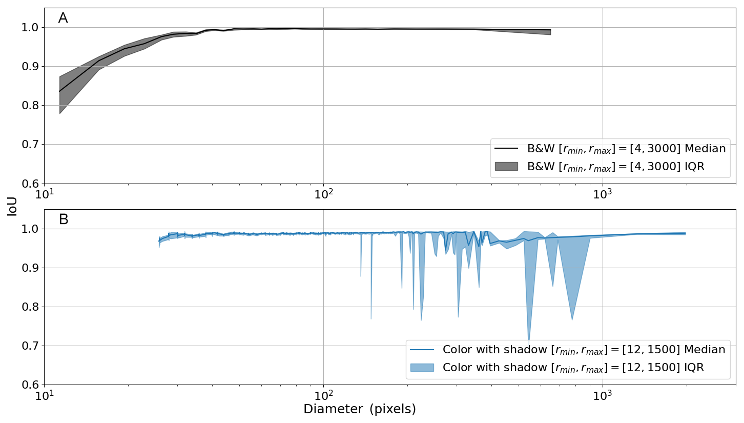
Figure 8 IoU statistics to measure mask quality. Labels are sorted by size and binned every 100 objects to calculate the median and IQR of IoU. The shaded area indicates the IQR. (A) Binned median IoU of the B&W scene shows high IoU with an average of 0.98. We note that objects with a diameter below ∼ 20 pixels generally have an IoU below 0.9. (B) Colored synthetic pebbles with shadow show an average IoU of 0.91. The variability of the IQR stems from pebbles partly in shadows.

The 27 528 synthetic colored pebbles with shadows were also binned to determine their precision, recall, and IoU. In general, the results are consistent with the B&W scene. For objects with a diameter above 30 pixels, recall consistently exceeds 0.9. With precision, we see a weak decreasing trend starting from a diameter of 100 pixels. The IoU consistently reveals median values above 0.9, but the IQR shows substantial variability, particularly in the lower quartile. Using colored scenes with shadowing shows that OrthoSAM is capable of reliably segmenting densely packed objects in a relatively large orthomosaic.

5.2 Grain-Size Distributions

We present grain-size distributions because this provides a link to field-based analysis. With the synthetic colored shadow scenes, we observe a close alignment with the ground truth data (Fig. 9). We performed the two-sample Kolmogorov-Smirnov test for goodness of fit (K-S) separately for each synthetic image (Hodges, 1958). In all cases, p-values exceed 0.25 (mean p=0.34, minimum p=0.27), indicating that the null hypothesis of identical distributions cannot be rejected, and the difference between the size distribution calculated from the OrthoSAM segments and the ground-truth size distribution of the objects is not statistically significant. Additional statistics for each experiment can be found in Table A4.

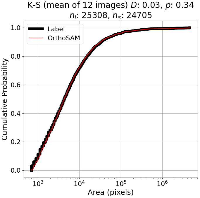
Figure 9 Cumulative probability distribution of ground-truth (black) and segmented (red) size distribution for n = 25 308 sysntetic pebbles from 12 colored scenes with shadows, thresholded at a detection limit of 30 pixels in diameter. Images were generated from a common base image with radius range $[r_{min},r_{max}]=[\mathrm{12},\mathrm{1500}]$ pixels, varying only the light source's azimuth and inclination. Out of 25 308 objects, OrthoSAM segmented 24 705 labels.

Through synthetic images, we have demonstrated that, in most situations, OrthoSAM effectively detects densely packed objects in large orthomosaics. It consistently produces high-quality masks (IoU > 0.9) for objects with a diameter greater than 20 pixels. Additionally, the segment size distribution accurately represents the actual size distribution for objects with a diameter greater than 30 pixels. After evaluating detection quality, mask quality, and segment size distribution, we observe that OrthoSAM produces consistently valid results. This is especially true for the synthetic cases, where segmentation quality is exceptionally high.

5.3 Ravi orthomosaics

Applying OrthoSAM, 973 objects were identified in Ravi2, 3231 in Ravi3, and 1880 in Ravi4 (Fig. 10). Grain-size distributions were computed with area, a-axis length, and b-axis length (Fig. A3). Across all measurements, Ravi3 and Ravi4 share a similar grain size distribution, whereas Ravi2 differs significantly from both.

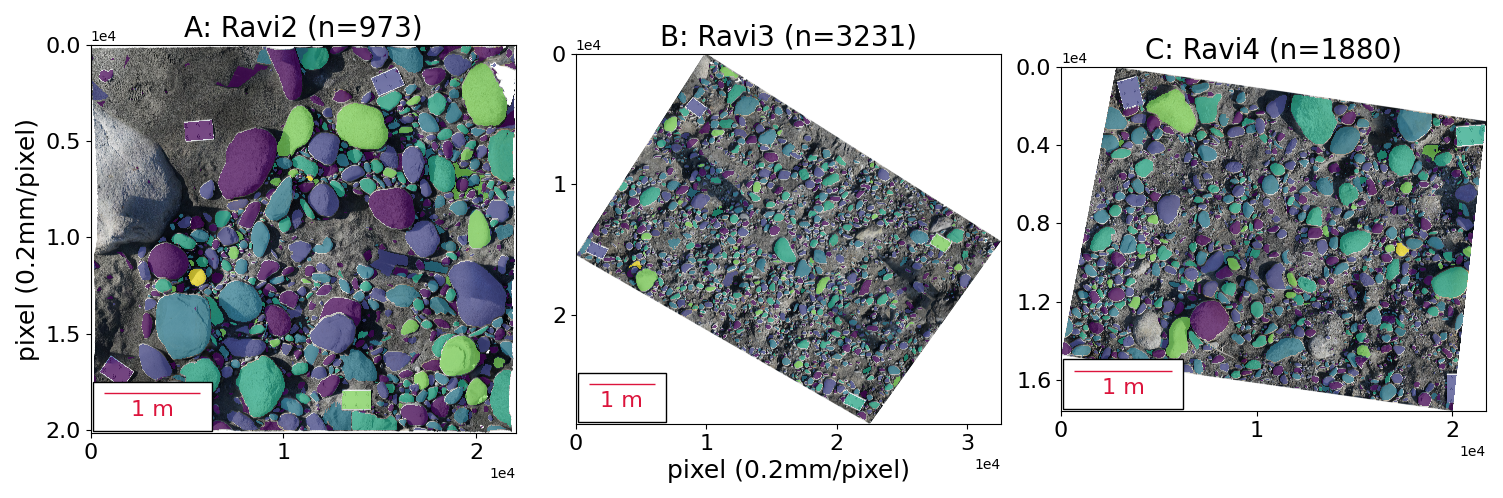
Figure 10 Segmentation results of the three Ravi River orthomosaics. Masks are randomly colored to distinguish individual objects. (A) 973 objects were segmented in Ravi2; (B) 3231 objects were segmented in Ravi3; (C) 1880 objects were segmented in Ravi4.

Due to the lack of precise ground-truth masks, IoU cannot be calculated for the Ravi datasets. Instead, predicted masks were manually screened to identify true and false positives based on whether the masked object was a pebble or not. All pebbles without a mask were also manually identified by comparing the image and the predicted masks. They were then classified as false negatives. The hillshade generated from the DEM was used to aid in manual validation. With false positives, true positives, and false negatives, precision and recall were calculated to assess performance (Table A5). The precision for all pebbles is 0.93, the recall is 0.94, and the overall AP is 0.97.

6 Discussion

In this section, we first discuss the size detection limit, noise tolerance, and the impact of shadows. Second, we will highlight typical problems and limitations of SAM and OrthoSAM. Finally, we discuss hardware requirements.

6.1 Noise Tolerance and Detection Limit of OrthoSAM

In Sect. 5.2, we have identified a lower detection limit of 30 pixels in diameter using the B&W scene. Above this limit, objects can be reliably detected and accurately segmented.

We have further investigated this limit by introducing noise and color. The results (Table A4 and Fig. A4) show that precision decreases with increasing noise (σ). The overall precision remains above 0.9 under moderate noise (σ<48). When exposed to strong noise (σ=96), the diameter of the object must exceed 40 pixels to achieve a precision of 0.9 (Fig. A5). Recall, on the other hand, does not show a clear correlation with σ, showing no statistically significant differences between noisy scenes and the baseline scene (σ=0). Suggesting that although false detection is significantly more likely with strong noise, the presence of noise does not overall impact OrthoSAM's ability to correctly detect objects.

For mask quality, the binned IoU was calculated and visualized for 3 different noise levels σ (Fig. A6). As the level of noise (σ) increases, we see a decrease in median IoU and an increase in IoU IQR. When exposed to extreme noise (σ = 192), the minimum diameter to ensure that IoU is greater than 0.9 increases from 20 to 30 pixels.

In summary, the detection limit of 30 pixels in diameter remains valid, given that noise is relatively moderate (σ<48). However, a high level of noise affects the accuracy and quality of the segmentation. Therefore, it is recommended to keep the ISO settings in a reasonable range during data collection to limit the noise. We emphasize that natural pebbles can exhibit large color variability as a result of different mineral specimens and lithology. In our synthetic examples, noise is introduced randomly, and there is a higher likelihood that noisy pixels will cluster into more coherent patches, particularly with a high sigma value. This can mimic the natural textural complexity of the pebbles. Through the Ravi orthomosaics, we observed that OrthoSAM is generally capable of handling this complexity; however, it is not flawless. The synthetic results support this observation: patches of noisy pixels within objects are sometimes misidentified as distinct objects, leading to an increased false positive count. This remains a common challenge in pebble delineation. Although the overall segmentation performance with the Ravi orthomosaics is satisfactory, this issue undeniably persists.

So far, our focus has been on the lower detection limit and noise, without addressing whether there is an upper limit. In principle, there is no upper detection limit, as the image can always be resampled to resize the object. There is a trade-off between strong resampling that will cause pixelation and lead to less accurate object boundaries, but doing so allows large objects to be segmented because they will fit into a single tile. However, we note that the tiling approach poses limitations on the object size (Fig. A7).

6.2 The impact of Shadows on Pebble Segmentation

In Sect. 5.2, we presented the segmentation assessment of synthetic scenes with and without shadows. We observed increased variability in mask quality with larger object sizes, mainly due to a decrease in the lower quartile (Fig. 8). This is also reflected in the precision (Fig. 7), suggesting that larger shadows are more frequently misidentified as an object. Although it seems counterintuitive, it is likely related to the tiling of the image. As the object size increases, the likelihood that it spans multiple tiles also increases, increasing the chance that the object intersects with tile borders. When this occurs, the full object mask is often discarded because of the intersection. Masks of shadow may remain, as it is likely to be smaller than the full object and more likely to be fully contained within a single tile. While coarser resolution layers, which likely involve stronger resampling, may successfully capture the complete object, these masks are typically excluded from the final output due to the prioritization of earlier layers (finer resolution in a fine-coarse setup as used in this study). In scenarios where strong and sharp shadows are expected, it may be advantageous to perform segmentation first at a coarser resolution before using a higher or original resolution.

Furthermore, we found that the extent of shadowing plays a significant role in model performance. Based on the proportion of an object's area covered by shadow, we categorized the objects into two groups: completely in shadow and partially in shadow. An object is considered completely in shadow if at least 90 % of its area is covered. We then repeat the previous analyses for each group separately. Interestingly, the model performed comparable to the shadow-free condition when evaluating only objects completely in shadow (Figs. A8 and A9). In contrast, objects partially in shadow were primarily responsible for the drop in precision and IoU observed in Figs. 7 and 8. This suggests that the stark contrast between the illuminated and shadowed regions within a single object may introduce ambiguity, making it more difficult for the model to segment the object accurately.

These findings indicate that the incorporation of appropriate preprocessing techniques could help mitigate this issue. Although we experimented with Contrast Limited Adaptive Histogram Equalization (CLAHE) on the Ravi orthomosaics and found that it did not lead to a significant improvement in our case, exploring alternative preprocessing methods remains a promising direction for enhancing performance under challenging lighting conditions.

6.3 OrthoSAM Limitations

In this study, OrthoSAM was applied to three characteristic examples of the western Himalaya (Ravi River), which were referred to as Ravi2, Ravi3, and Ravi4. In general, the pebbles in the three orthomosaics exhibit a similar size composition (Fig. A3). With the only exception that Ravi2 does contain a higher number of larger pebbles.

The predicted masks were manually inspected and assessed due to the lack of ground truth data. Overall, we see good precision, recall, and AP (Table A5). However, there are a few caveats to consider.

First, manual validation is inevitably prone to subjectivity and human error, leading to potential biases and inconsistencies. Therefore, the validation of the proposed method and the assessment of mask quality mainly rely on synthetic images, for which ground-truth data is available. We emphasize the need for a good validation dataset for digital pebble sieving. We explored additional validation datasets, such as three images (S1, FH, and K1) from the ImageGrains v1 dataset (Mair, 2023; Mair et al., 2024). While this dataset provides manually annotated labels, these are only available for a subset of cropped patches from the original images. As a result, the evaluation was limited to a qualitative assessment. Visual inspection of segmentation results on ImageGrains images suggests that OrthoSAM generalizes well to unseen datasets beyond the Ravi River dataset on which it was developed. OrthoSAM was applied using two parameter settings: (1) parameters specifically adjusted after visual inspection of each image, and (2) the default parameters designed for standard large images (for details of the parameter settings, see the GitHub repository). While the default configuration already shows good performance, smaller objects are more frequently missed (Fig. A10). Nevertheless, the resulting grain-size distributions remain consistent across both parameter settings (Fig. A11), despite differences in the total number of detected objects. This suggests that while parameter tuning improves segmentation completeness, OrthoSAM can still recover comparable size distributions using its standard configuration. Finally, we emphasize the importance of developing a community-based reference dataset for granular material segmentation. Such a dataset would be analogous to widely used benchmark datasets in the lidar and point-cloud communities and would facilitate more standardized and quantitative comparisons between methods.

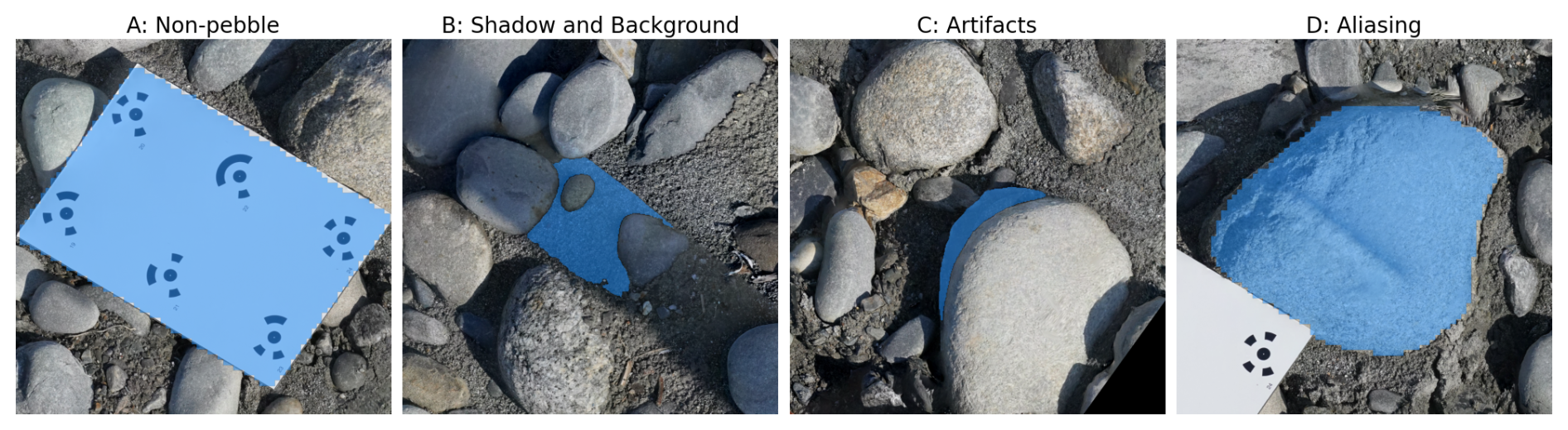
Figure 11 Four examples of common segmentation issues taken from Ravi3. The blue area indicates the masked area. (A) Segmentation is correctly performed, but the segmented object is not a pebble; (B) shadow and background mistakenly segmented as an object; (C) Structure-from-Motion artifacts due to image mosaicing issues that can be mistaken as an object; (D) aliasing effect caused by resampling a segmentation completed at a coarser resolution back to the original resolution.

Second, it is important to remember that SAM only performs instance segmentation. OrthoSAM is a workflow designed to assist SAM in delineating densely packed objects in large, high-resolution images. However, it does not incorporate any object classification algorithm or semantic segmentation model, although this could be explored in future improvements. As a result, non-pebble objects are also delineated. In the Ravi orthomosaics, various non-pebble elements, such as A4 marker panels and wooden branches, were also segmented (Fig. 11). Measurements, metrics, or statistics calculated without first removing the corresponding masks could lead to inaccuracies. The significance of this issue depends on the abundance of irrelevant objects. Simple filtering steps based on color or $a/b$ axis ratio may remove these masks. An alternative approach taken in Segmenteverygrain (Sylvester et al., 2025) is to develop a convolutional neural network to identify pebbles and place seed points for SAM to delineate. This effectively filters out irrelevant objects but relies on the CNN to identify pebbles in the first place.

In addition to these limitations, false detections due to structure-from-motion (SfM) artifacts, image distortions, and shadows were also observed in the final segmentation results of the Ravi orthomosaics (Fig. 11). Ravi orthomosaics are 2D projections of the 3D reconstruction created with Metashape through SfM. This allows us to create a high-resolution orthomosaic of a large area. The issue with orthomosaics is that there can be artifacts caused by image fusion issues such as mismatched pixels, insufficient image coverage, moving objects, or changes in lighting. This issue is particularly noticeable at the edges of the orthomosaic, where insufficient image coverage prevents an accurate 3D reconstruction. With the most updated SAM checkpoint, these artifacts would still interfere with segmentation, and they can be mistaken for an object.

6.4 Application

The core motivation of this study is to create a SAM-based workflow that allows efficient and automated photo-sieving and the processing of large sample sets. The segmentation results allow us to extract grain size data and calculate various measurements and statistics that can be used for grain size analysis. To demonstrate the potential application, several measurements and statistics were calculated. As an example, the normalized isoperimetric ratio (IRn) (e.g., Pokhrel et al., 2024) was calculated to provide an evaluation of pebble roundness (Fig. A12). For the Ravi orthomosaics, IRn shows that all three orthomosaics are composed of pebbles with consistent roundness.

We strive to provide a tool that allows the rapid generation of multiple metrics relevant for grain-size analysis. We include common grain size measurements such as area, a- and b-axis lengths, perimeter, and mean and median R, G, B values (Table A6). The output is generated as a dataframe and can be stored in a transferable format for further processing, such as clustering analysis using the RGB statistics.

We make the following suggestions for field-data collection efforts: Due to the significant difference in performance, it is recommended to consider the detection limit during data collection. The image resolution or camera distance should be selected to ensure that the smallest pebble size to be detected has at least a diameter of 30 pixels. As every camera and sensor has different noise performance, it is recommended to generate a noise image and take a series of testing photos at different ISO settings to determine the corresponding ISO value that will lead to high noise levels. However, most modern cameras provide excellent (low) noise levels even at higher ISO values. Reliance on RGB information for segmentation implies that strong contrast, changes in lighting conditions, and processing artifacts can influence the result of segmentation. During data collection, these factors should be taken into account.

6.5 Hardware Requirements

As a vision transformer-based model, SAM heavily relies on GPU computing power and memory (Yu et al., 2023). Our approach was developed and tested on an NVIDIA Quadro RTX 5000 GPU with 16 GB of memory, a powerful but costly GPU that may not be accessible to all potential users. The segmentation of a synthetic image with 10 000 × 10 000 pixels requires approximately 4 h, whereas an image with 2048 × 2048 pixels requires about 5 min. Without a powerful GPU, the processing of segmentation will take longer. In addition, insufficient GPU memory can significantly degrade performance. As discussed in Sect. 4.2, each delineated object must retain its own binary mask throughout the process until the untiling step. This requires storing up to the number of input points × 3 layers of 1024 × 1024 boolean arrays (assuming the tile size is 1024 × 1024 pixels) in GPU memory. The memory demand thus scales non-linearly with the number of input points (Fig. A13). However, the number of input points is a critical parameter as it determines the number of discoverable objects in the initial step at each resolution layer. Therefore, the performance is ultimately constrained by the availability of GPU memory.

7 Conclusion

We present a novel tiling and merging approach, including a new input point generator for the Segment Anything Model (SAM) to process large orthomosaics. We refer to this workflow as OrthoSAM. Our approach enables users to perform grain-size analysis on virtual outcrops with a large number of pebbles (> 10 000 objects). We carefully validated our methodology with synthetic pebble images and hand-clicked orthomosaics from field images.

Fluvial pebbles exhibit a wide range of sizes that exceeds the original purpose of SAM. Large pebbles may not be able to fit into a standard 1024 × 1024 pixel tile at the original image resolution. We developed a multi-resolution approach that enables OrthoSAM to handle different size ranges through rescaling (or resampling). For example, the down-sampling or coarsening step allows larger boulders that do not fit into a standard tile to be identified.

We identified a lower detection limit of 30 pixels in diameter. That is ∼ 700 pixels or 28 mm² with a spatial resolution of 0.2 mm per pixel, assuming a circular object. With a spatial resolution of 1 mm per pixel, the size limit in metric units will increase to 7 cm². For grains with a diameter above the limit, we expect the recall and average IoU to be above 0.9, and the segment size distribution to reflect the actual size distribution.

A validation effort using synthetic images with 27 528 colored circles and shadows shows that OrthoSAM has achieved a precision of 0.98, a recall of 0.94, and an average IoU of 0.91. The synthetic orthomosaic reveals the impact of shadowing on segmentation performance. Specifically, synthetic objects that are partially covered by shadows exhibit lower precision and IoU due to the boundary between the lit and shadow sides. In contrast, those completely covered by shadow are consistently and accurately segmented, suggesting the importance of uniform lighting conditions during data collection. Appropriate pre-processing techniques could mitigate this issue.

OrthoSAM was applied to three orthomosaics from the western Himalaya with a wide range of grain size. Validation shows an average precision of 0.92 and an average recall of 0.95. In total, 6087 pebbles were delineated. The projected area ranges from 10 to 927 cm².

We developed a Python-based software pipeline that generates a table (dataframe) with relevant metrics for further grain-size analysis, available on GitHub (https://github.com/UP-RS-ESP/OrthoSAM, last access: 15 March 2026) and archived on Zenodo (https://doi.org/10.5281/zenodo.19411461, Chan et al., 2026).

Appendix A: The Segment Anything Model (SAM)

The Segment Anything Model (SAM) is an efficient and promptable model for image segmentation. SAM was trained with over 1 billion masks in 11 million licensed and privacy-respecting images and generates good segmentation results without additional training (Kirillov et al., 2023). SAM allows segmentation of a broad set of use cases and can be applied out of the box on new image domains without additional training, including scientific images such as cell microscopy or pebble images (Na et al., 2024; Israel et al., 2023). This capability is referred to as zero-shot transfer. Thus, SAM's zero-shot performance is often competitive with or superior to prior fully supervised results. SAM has been developed as an image segmentation tool that allows input through multiple prompts, such as user queries through clicking, outlining polygons, or text input. A typical application is to cut an object (e.g., a person) from the foreground of an image and replace the background. Other applications take advantage of SAM's recognition quality, such as “identify all cats in this image”. None of these use cases is directly applicable to fluvial pebble segmentation, but the trained SAM model provides unique capabilities to segment pebbles in images with shadows or complex lighting. We leverage SAM because of its unique ability to segment a wide range of image types, including complex lighting conditions and conglomeratic boulders. Specific, custom-trained deep-learning models may perform excellently for the settings they have been trained for, but often perform weaker when boundary conditions such as light, color, size, and shape of pebbles change. The wide range of fluvial sediment shapes and their size range stretching over several orders of magnitude, from mm (sand) to m-sized boulders, provides a challenging training environment. To our knowledge, no such training dataset exists, and it will be difficult to generate this given the complex lithologies and processes of mountain rivers.

SAM's unique ability lies in its zero-shot inference. This means that SAM can accurately segment images without prior specific training, a task that traditionally requires tailored models. This has been achieved by training the model with a large number of images and generating a large number of parameters. In addition, a new model architecture with three decoupled components: image encoder, prompt encoder, and mask decoder provides an efficient framework where multiple tasks can be performed on an encoded image. The image encoder is responsible for processing and transforming input images into a comprehensive set of features. The encoder compresses the images into a dense feature array. This array forms the base from which the model identifies various image elements and is the core output of the learning approach. The prompt encoder interprets various forms of input prompts, such as text based, points, polygon masks, or a combination thereof. This encoder translates the prompts into an embedding that guides the segmentation process. For example, a prompt can be a point that is clicked on a pebble that is then delineated. The density of points determines the number of objects that are segmented. The prompt encoder enables the model to focus on specific areas or objects within an image. The mask decoder performs the actual segmentation steps, and it synthesizes the information from both the image and the prompt encoders to produce a segmentation mask. Both Convolutional Neural Networks (CNNs) and Generative Adversarial Networks (GANs) play an important role in the capabilities of SAM. Although CNNs provide a robust method for feature extraction and initial image analysis, GANs are used to generate accurate and realistic segmentations.

SAM: Workflow, Limits, and Strategies

This framework allows SAM to understand a wide array of visual inputs and respond with high precision. There are several important boundary conditions to note when using SAM to process images for fluvial pebble segmentation. The input data for the delineation of the pebbles are usually large orthomosaics generated from hand-held cameras (e.g., Purinton and Bookhagen, 2021) or UAV images (Mair et al., 2022). SAM rescales all input images to 1024 ×  1024 pixels to fit the transformer architecture – a large image with several thousand pixels in width and length will be rescaled when processed by SAM. The prompt encoder requires input points to identify objects. Input points can be thought of as a coarser raster draped over the input image to identify points of interest: The finer the scale of this raster, the more grains can be detected (Fig. 1). The standard SAM model applies 32 × 32 equally spaced input points in the standard, automated detection scheme. The transformer and prompt encoder were optimized for a limited number of objects, not hundreds to thousands of objects per image, as would be the case for pebbles on a large orthomosaic. A hardware limiting factor for the spacing of input points is GPU memory because high input point densities (i.e., a closely spaced grid) will require a large amount of GPU memory (Fig. A13). For example, a 1024 × 1024 image allows for a maximum of 73 points for each length and width (total of 5329 input points) with a 16 GB GPU. The reason for the high memory usage is that every input point results in three masks (whole, part, and subpart) at the original input image resolution. This generates up to 15 987 masks if no filtering is applied, and SamAutomaticMaskGenerator needs to retain all generated masks in memory for post-processing steps. This multi-masks output (whole, part, and subpart) is a SAM mechanism developed to tackle the ambiguity of defining an object (Fig. 1). The input point density is thus a limiting factor for densely packed object delineation. Only large and currently expensive GPUs (in the year 2025) can perform calculations with higher input point spacing, but detecting patches with multiple small object sizes will remain a challenge with this approach.

Pebble detection through SAM is therefore limited by hardware resources. SAM has not been designed to detect densely packed objects such as pebbles or sand in high-resolution images. A common strategy for image analysis with SAM is to generate an input point grid that delineates objects at the input point location. In a second iteration, the point grid can be shifted to detect missed objects. An alternative strategy is to subset the original image. For example, a tiling approach allows for increasing the number of objects detected: A 1024 × 1024 pixel image tiled into four 512 × 512 pixel images and then each upscaled to 1024 × 1024 to fit the encoder will result in a denser spacing given the same original input point spacing. A third strategy is to use an alternative method, such as manually clicking on the input point location, to identify a specific section within the pebble. Manually clicked input points anywhere within a pebble will lead SAM to extract each pebble. This will turn SAM into a successful region-growing tool. Similar semi-automatic approaches were suggested by Purinton and Bookhagen (2019). Although this will significantly speed up pebble delineation as compared to manually delineating pebbles, it is an unsatisfactory approach that does not take full advantage of automation procedures. In the presented approach, we develop a tiling and resampling scheme to ensure that all parts of the image are covered and that pebbles are detected on various image scales.

Table A1 Summary of parameters used to generate three sets of synthetic images with 10 000 × 10 000 pixels each.

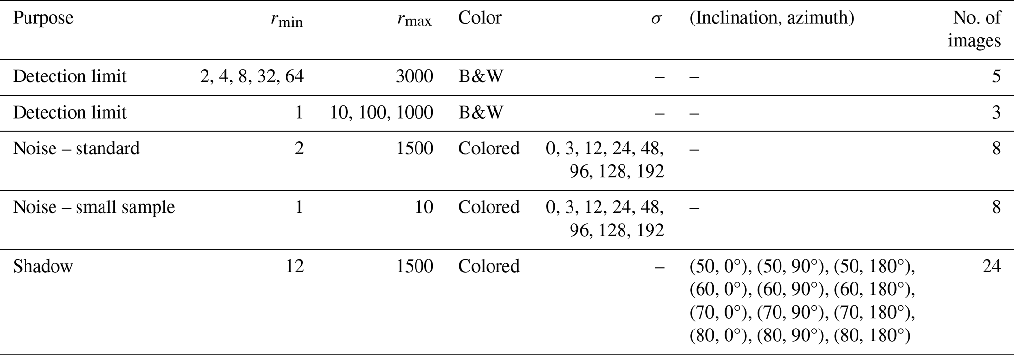
Table A2 Summary of OrthoSAM parameters used for the segmentation of synthetic images and Ravi orthomosaics.

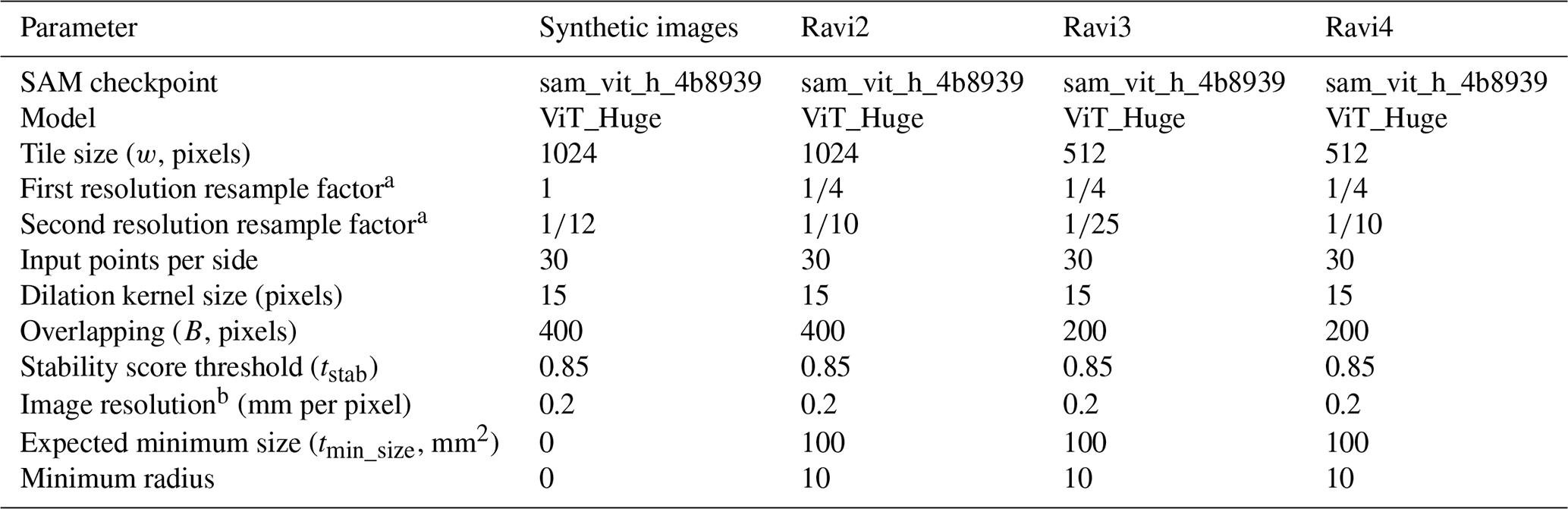
^a Scale factor along both horizontal and vertical axes. ^b For the synthetic images, resolution is used only to convert the expected minimum size from metric units to pixels.

Table A3 Colored synthetic scenes and their OrthoSAM delineated object count using the described tiling and merging approach sorted by their noise levels (σ).

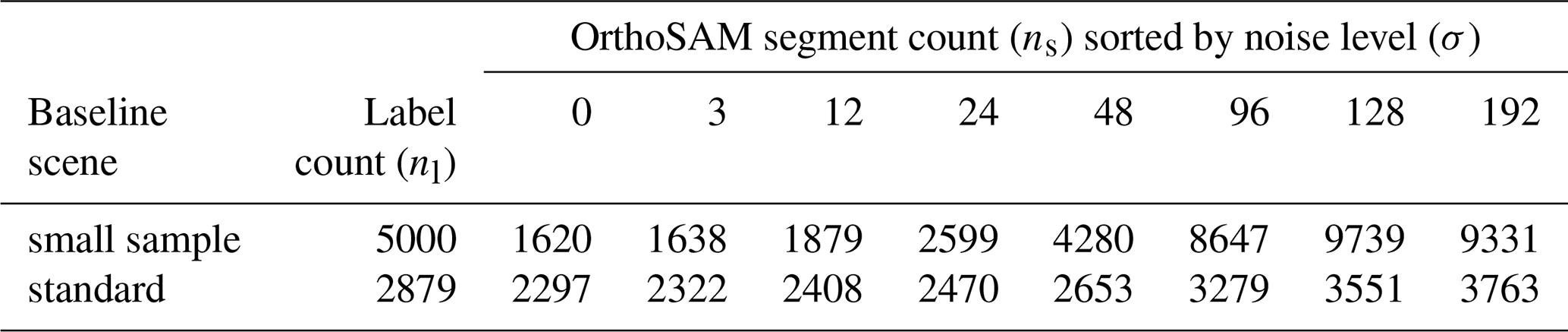
Table A4 Detection quality evaluation of colored synthetic scene segmentation with two-sample Kolmogorov-Smirnov test (K-S) and mean IoU. K-S_t is thresholded by the detection limit (diameter > 30 pixels). Small sample scene (SS): $[r_{min},r_{max}]=[\mathrm{01},\mathrm{10}]$, n_l = 5000. Standard scene (ST): $[r_{min},r_{max}]=[\mathrm{01},\mathrm{10}]$, n_l = 2879. SS has no sample after thresholding.

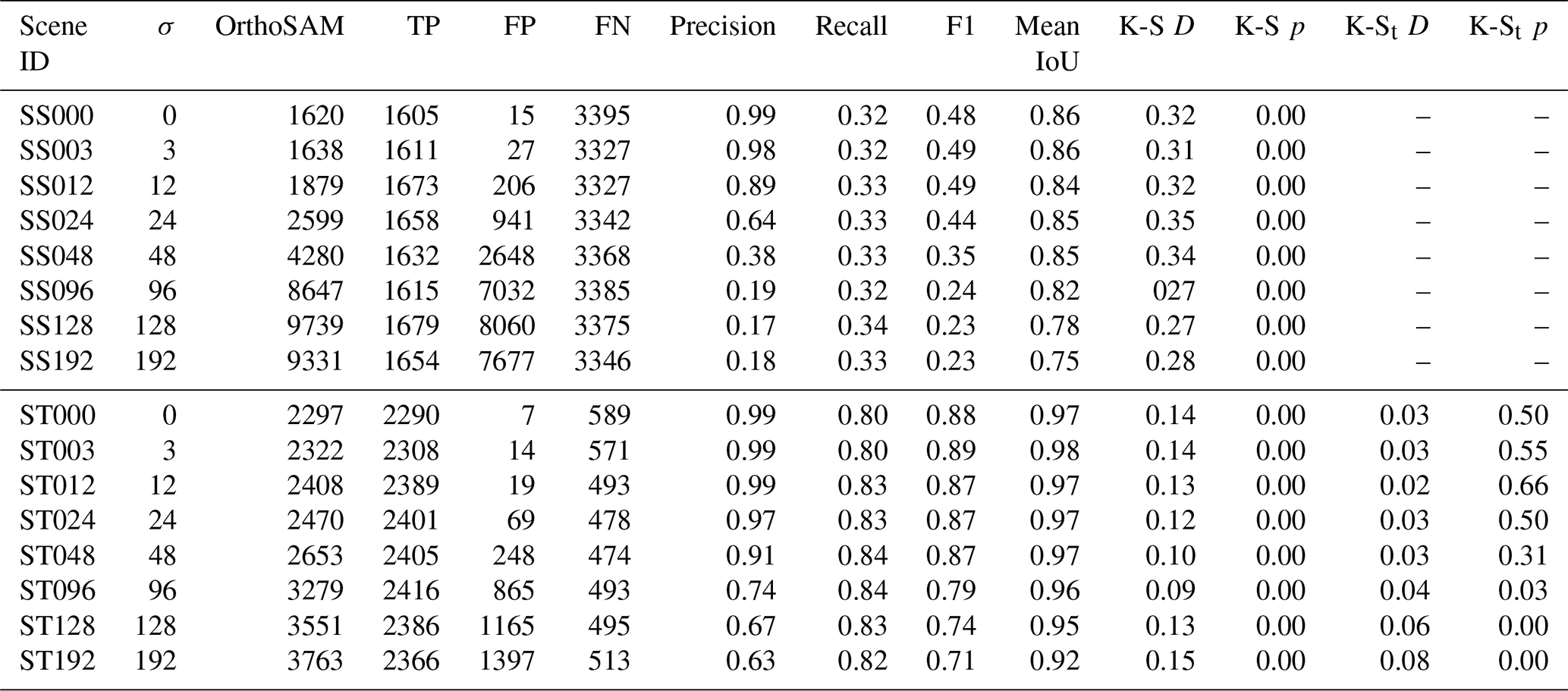
Table A5 Ravi image performance assessment with the number of detected pebbles.

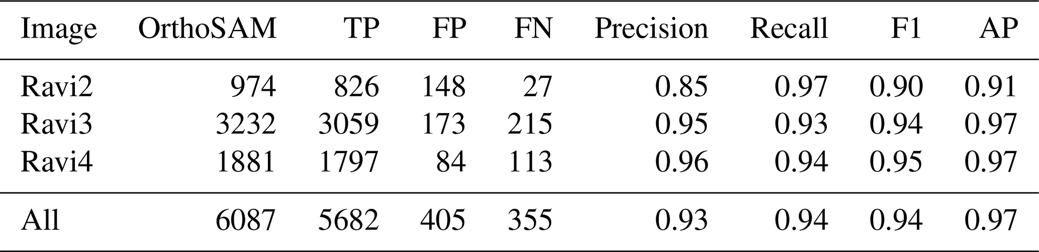
Table A6 Grain size data example output. The grain size dataframe contains the x and y coordinates of the centroid, the area (mm²), a-axis length (mm), b-axis length (mm), perimeter (mm), normalized isoperimetric ratio (IRn), mean RGB values, and median RGB values. Instead of RGB, color statistics can also be calculated for other color spaces by converting the input image.

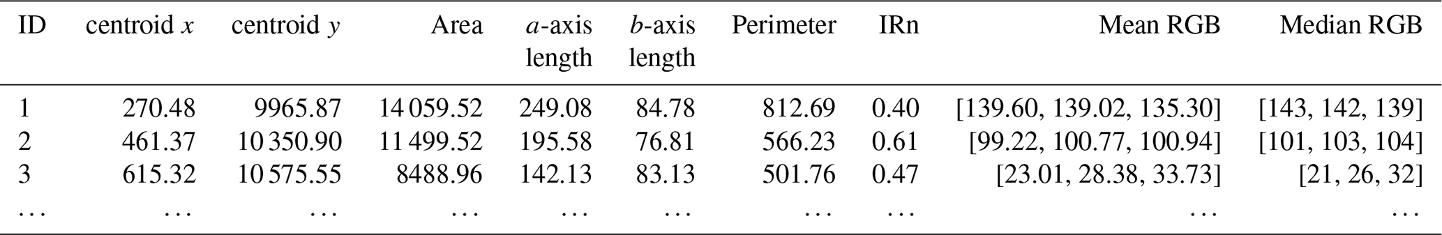
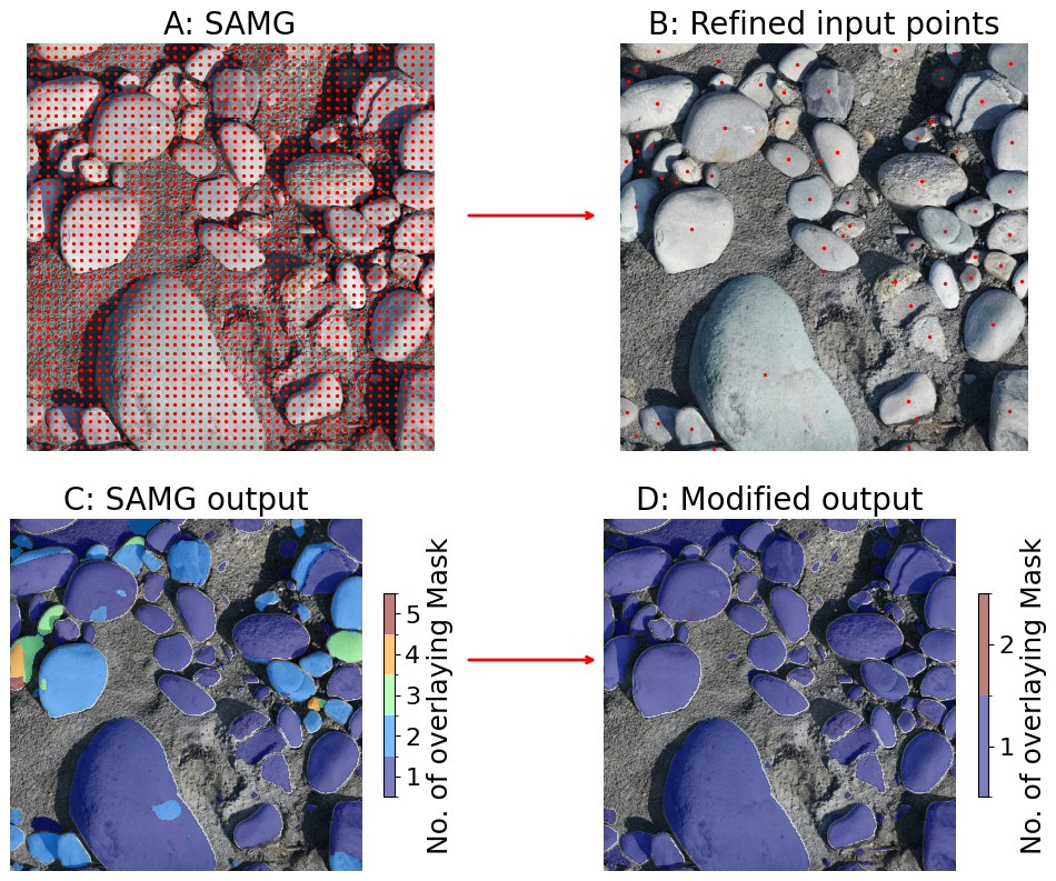
Figure A1 Input point generation workflow. Using the SamAutomaticMaskGenerator (SAMG), the initial 48 × 48 equally spaced input points (A) generate an output mask (C) with larger pebbles showing multiple masks; (B) The improved workflow refines the input point to one input point per object to reduce mask count and optimize GPU memory usage. The number of multiple mask counts due to multiple input points is greatly reduced through our modified approach. This is a prerequisite step to successfully apply SAM to large orthomosaics.

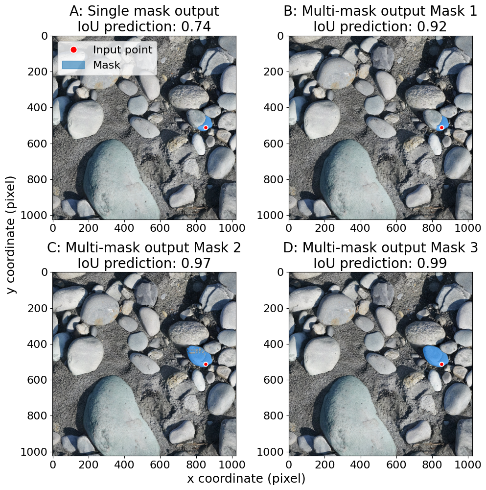
Figure A2 A characteristic example using SAM's capability to delineate a single pebble with a single input point. The image has 1024 × 1024 pixels with a resolution of 0.2 mm per pixel. SAM produces three output results termed masks (whole, part, and subpart masks). When a single mask is desired, the SAM developer team recommended selecting the mask with the highest IoU prediction. The SamPredictor has the option to output a single mask only (A), which will be the first mask predicted. As the single mask output option does not always return the mask with the highest IoU score, it is recommended to use the multiple mask output option and select the mask with the highest IoU score. This sample illustrates the variety of output masks generated by SAM for a single prompt point.

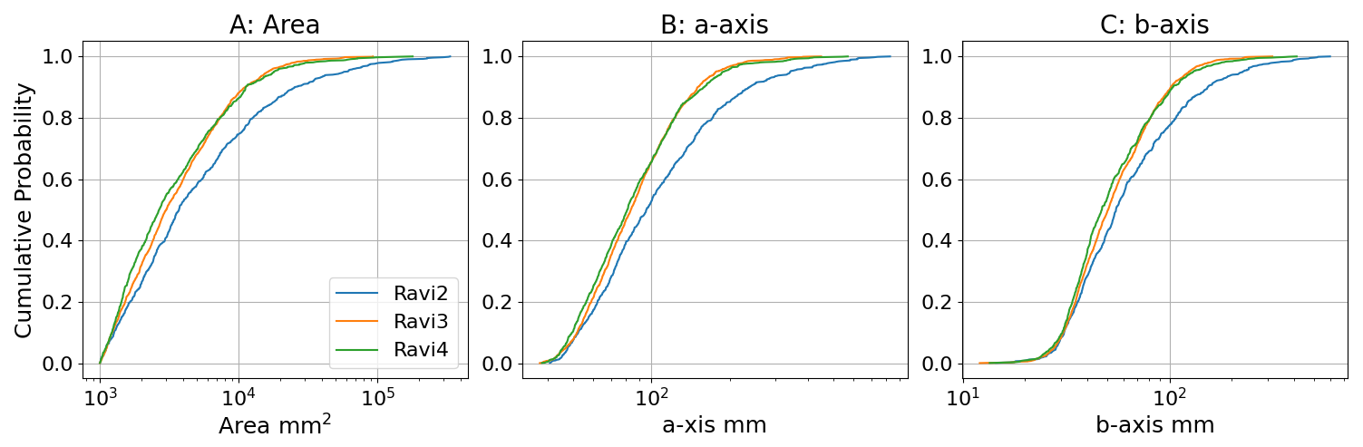
Figure A3 Cumulative grain size distribution of the three Ravi scenes. (A) area distribution; (B) major axis distribution; (C) minor axis distribution.

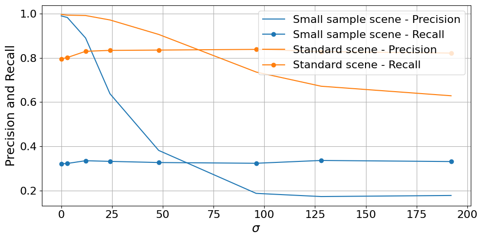
Figure A4 Precision and recall of segmentation of the synthetic color scene. Small sample scene (n_l = 5000): $[r_{min},r_{max}]=[\mathrm{01},\mathrm{10}]$. Standard scene (n_l = 2879): $[r_{min},r_{max}]=[\mathrm{01},\mathrm{10}]$. The small sample scene is created to simulate densely packed small objects, and the standard scene is created to simulate Ravi orthomosaics. σ describes the Gaussian noise level.

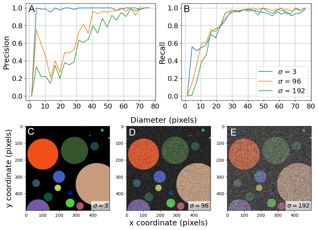
Figure A5 Binned precision and recall for colored synthetic scenes with noise. Labels are grouped by diameter into 3-pixel bins to compute recall within each range. (A) Precision. (B) Recall. Three level of noise were applied and visualized to provide a reference. (C) Minimal noise: σ=3. (D) Strong noise: σ=96. (E) Extreme noise: σ=192.

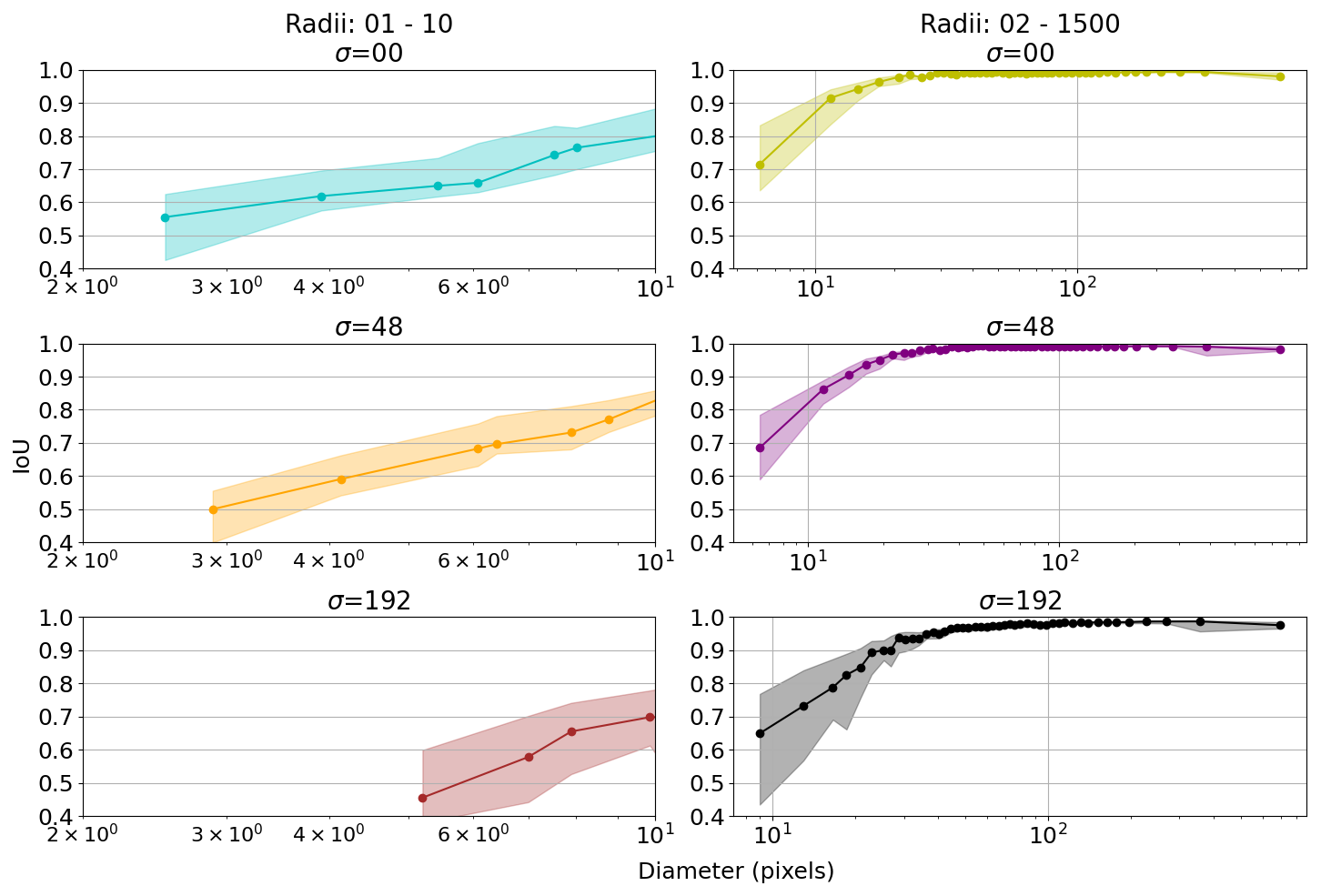
Figure A6 Effect of noise level σ on binned median IoU of colored scenes. IoU was sorted by label size and binned every 50 samples to calculate the median and IQR. The symbol marks the mean area within the bin. The shadowed area indicates the IQR.

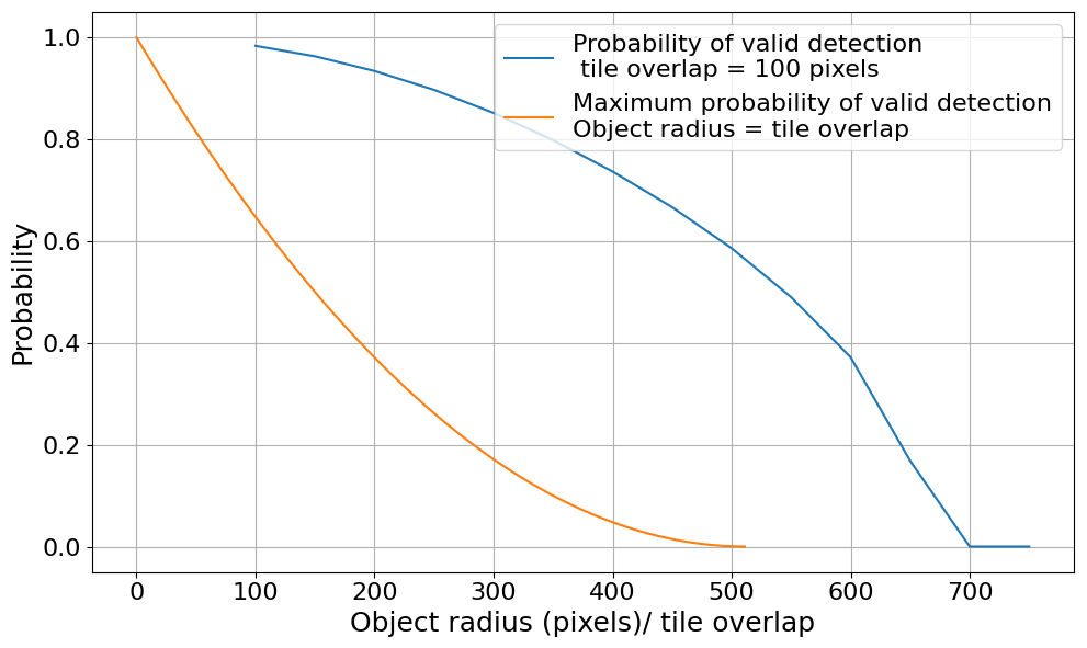
Figure A7 Probability of valid detection assuming tile overlap of 100 pixels and maximum probability of valid detection assuming an object radius equals tile overlap. Objects are assumed to be perfectly circular when calculating the probability.

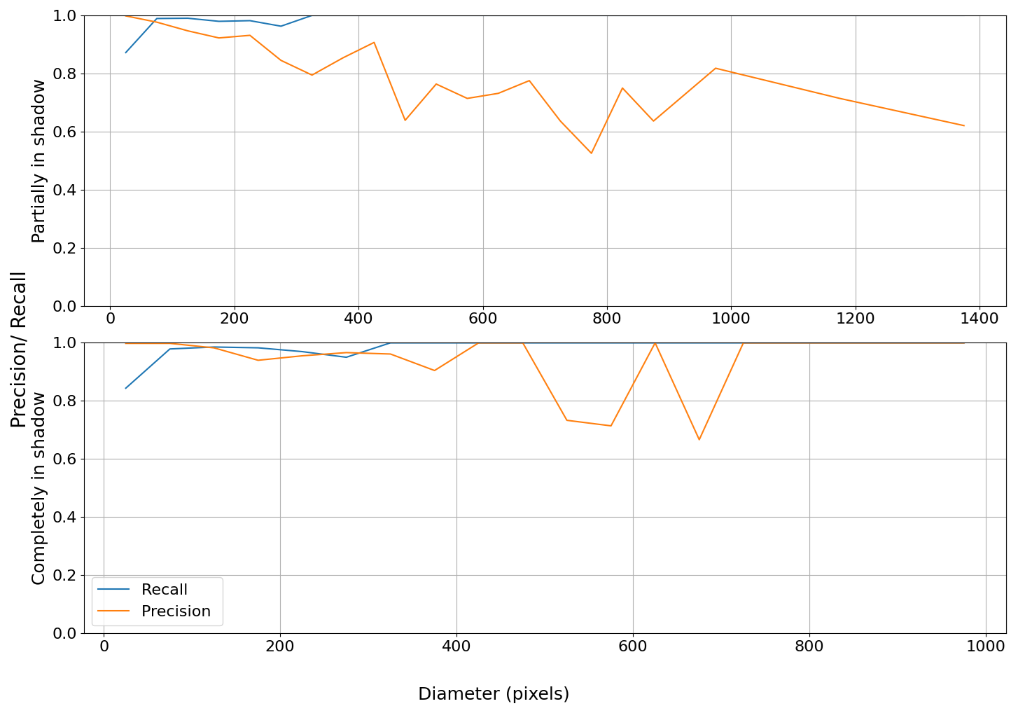
Figure A8 Binned precision and recall of synthetic objects partially and completely in shadows (n = 27 528 pebbles). Labels are grouped by diameter into logarithmic bins to compute precision and recall within each bin.

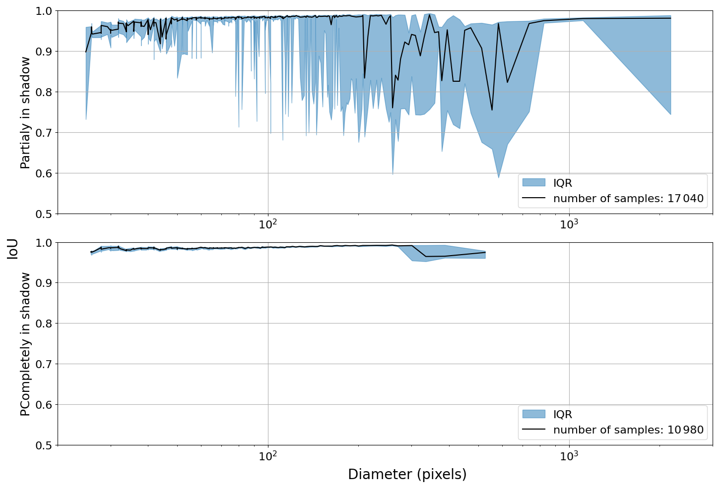
Figure A9 IoU statistics to measure mask quality. Labels are separated into partially in shadow and completely in shadow, sorted by size, and binned every 100 objects to calculate the median and IQR of IoU.

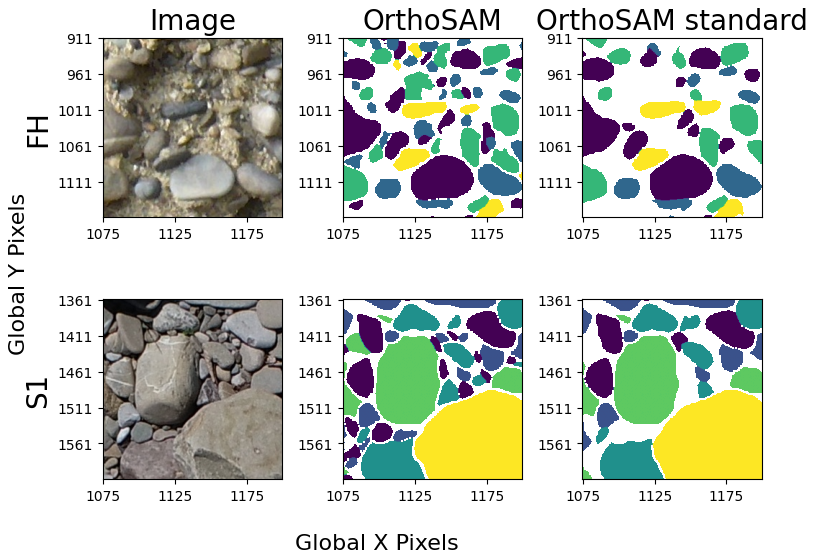
Figure A10 OrthoSAM (OS) predictions for center crops of FH and S1 images from ImageGrains v1 dataset (Mair, 2023; Mair et al., 2024). OrthoSAM predictions were made with two different settings: custom parameters for the respective image and standard parameters for large images. The number of identified objects varies between the methods, with custom parameters detecting more objects than standard parameters. For example, for image S1, the custom parameters prediction identified 4316 objects whereas standard parameters prediction only identified 2915 objects. While the ImageGrains dataset provides ground truth labels, these are only available for a subset of cropped patches from the original images. This does not allow a precision and accuracy assessment with the same training data. Both prediction demonstrated OrthoSAM's capability in delineating densly packed objects. However, custom parameters specifically adjusted after visual inspection of each image outperforms default standard parameters in detecting very fine objects. Additionally, due to the lack of a classification component, OrthoSAM has the inherent limitation that irrelevant objects may remain in the segmentation results. In particular, we see patches of sand that were falsely segmented in FH. Here, we see that lower resolution or blurriness in the image can exaggerate the issue, resulting in more false positives.

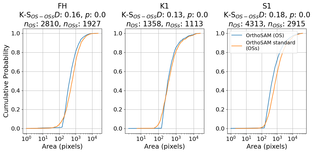
Figure A11 Cumulative size distribution of OrthoSAM predictions for images FH, K1, and S1. OrthoSAM predictions were made with two different settings: custom parameters for the respective image (OS) and standard parameters for large images (OSs). The number of identified objects varies between the methods, with OS detecting more objects than OSs. A two-sided K-S test was performed to compare the similarity of the size distributions. For all images, the null hypothesis that the samples come from the same distribution was not rejected (p>0.05), indicating that the segment size distributions produced by two settings do not differ significantly. This suggests that while parameter tuning increases the number of detected segments, the overall grain-size distribution extracted by OrthoSAM remains consistent.

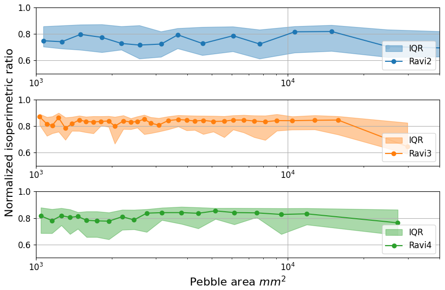
Figure A12 Normalized isoperimetric ratio (IRn) of the three Ravi orthomosaics. IRn was sorted by label size and binned every 50 samples to calculate the median and IQR. The points identify the mean area within the bin.

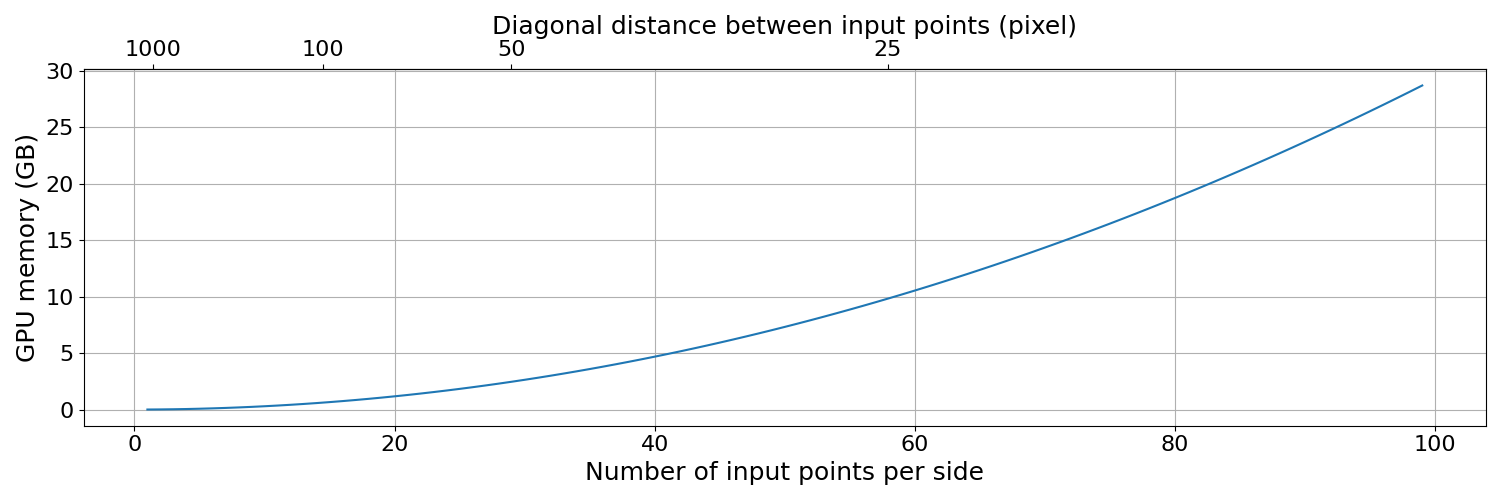
Figure A13 Memory demand for 1024 × 1024 pixel image by the number of input points per side (n_pps) and the diagonal distance between input points. This estimate is based on the memory required to store $n_{\mathrm{pps}}^{\mathrm{2}}$ × 3 binary masks in the memory. However, the actual memory requirement may be higher due to additional overheads not accounted for in this calculation.

Appendix B: Synthetic Pebble Generator

Synthetic scenes are generated at a resolution of 10 000 × 10 000 pixels to achieve a scale comparable to that of real-world orthomosaics. Within these images, solid circles of random sizes are placed randomly. The placement process begins by determining the size of each circle, where the radius (r) is randomly sampled from a uniform distribution over a predefined range $[r_{min},r_{max}]$. Once the size is set, a random point in the image is selected as the centroid. Before placing the circle, we check for potential overlap with existing circles to ensure that no circle will directly touch a neighboring circle (at least one pixel distance). Without this gap, two touching circles of the same color would be indistinguishable, making it impossible to segment them correctly as separate objects. If this requirement is not met, a new location is randomly selected. This process continues until a valid placement is found or until 100 attempts have been made. If no valid placement is found after 100 attempts, the circle is discarded. This process is repeated 5000 times, which creates up to 5000 solid circles. Due to the randomized placement strategy, synthetic images generated with the same set of parameters may contain a different number of circles. This approach ensures diversity in the dataset while maintaining a controlled testing environment.

Synthetic images were generated in B&W, colored, colored with noise settings, and shadowed settings. B&W scenes consist of black backgrounds and white solid circles; they were created to determine the range of object sizes that can be accurately segmented by SAM. The simplicity of B&W images allows us to isolate size as a key factor, minimizing the influence of other variables. Filling solid circles with random colors provides us with noise-free, colored synthetic scenes, which better approximate reality. Based on the noise-free colored synthetic scene, we can further introduce different levels of Gaussian noise to simulate digital noise. The level of noise introduced was controlled through the standard deviation parameter (σ) with the mean set to 0. The introduction of noise creates a more realistic image, which enables us to assess the robustness against noise.

Examples of the synthetic pebble generator are shown in Figs. 2 and A6. The source code of the synthetic pebble generator is included in the github repository (https://github.com/UP-RS-ESP/OrthoSAM).

Appendix C: Methodology: Tiling of Input Images

Internally, the SAM model will always rescale and pad the input images to a 1024 × 1024 pixel resolution. For images larger than 1024 × 1024, such an operation will inevitably lead to a loss of information. For a 24 MP camera commonly found today, the images typically have a resolution of approximately 6000 × 4000 pixels. To fit this image into a 1024 × 1024 box without altering its aspect ratio will drastically reduce the megapixel count from 24 to roughly 0.7. A resolution of 0.7 MP is generally sufficient for segmentation, especially considering that photos taken in daily life often feature clear, well-defined objects that occupy a significant portion of the image. This is no longer the case when we consider large orthomosaics with thousands or more individual pebbles. A pebble of 100 × 100 pixels on a 20 000 × 20 000 pixels image will only occupy a 5 × 5 pixels large box after rescaling the image to 1024 × 1024 pixels. As a consequence, smaller objects are more likely to be overlooked, and larger objects may suffer from reduced masked quality (Fig. 5). Even if we are willing to accept these compromises, the image size also poses limitations on the number of detectable objects. A tiling approach is necessary for large images and images that contain a large number of objects.

Let w be the window size. By default, we tile images into 1024 × 1024 pixel patches, matching the input resolution of the transformer. Tiling will inevitably cut through the samples (pebbles). Thus, between each adjacent tile, there is an overlap of B pixels. This offers the additional advantage of a higher input point density, reducing the probability of overlooking objects. The issue is that, unless there is a considerable amount of overlap, it is almost certain that window borders will cut through at least some pebbles. The result is a trace of artificially over-segmented pebbles along the tiling edges. To avoid this from happening, masks will be discarded if they touch the window border. Additionally, a valid box was introduced for filtering to ensure that only one mask would be generated for each sample. The valid box is a 1024-B × 1024-B window located in the center of the tiles, so it should always be $\frac{B}{\mathrm{2}}$ pixels away from the window edge. A mask will only be kept if at least 50 % of the masked pixels can be found inside the valid box. This can effectively avoid duplicating masks due to the overlap of windows at the cost that fairly sized samples may not be segmented at all. In Sect. 4.3, we will present how this issue can be solved.

Once tiled, each patch will be processed further. The final product will then be untiled and combined into a 2D-labeled mask.

SAM is capable of delivering high-quality results straight out of the box, but it is also obvious that SAM was not intended to delineate pebbles from large orthomosaics. A photo taken for photo-sieving differs from everyday photos in various ways. Compared to everyday photos, it lacks a clear main subject, as most of the things captured in the image are the main subjects. It contains more objects than usual, which may be more densely packed and vary significantly in size. This leads to the challenge of coming up with an input point grid that is capable of picking up all objects that we are interested in. A fine grid minimizes the risk of missing smaller objects. However, it also causes larger objects to receive an excessive amount of input points. This leads to a high number of duplicate masks. While this issue can be addressed using non-maximum suppression, this also leads to an increased probability of over-/under-segmentation. The increased likelihood of over-segmentation is a problem that non-maximum suppression cannot resolve. This issue stems from how SAM resolves the ambiguity of objects, which is to predict three masks at three different levels (whole, part, and subpart). Although this tactic to tackle the ambiguity of objects is effective in handling objects with multiple layers, it also increases the likelihood of errors when segmenting single-layer objects like pebbles. The placement of input points further contributes to this variability in the segmentation results. For example, if we have a partially shadowed pebble where a third is in a shadow and the rest is properly lit, the differences in lighting will create a strong contrast. SAM may over-segment the pebble if the input point lands around the center of either part. With more input points landing on the pebble, the likelihood of generating an over-segmented mask increases. In contrast, using a coarser input point grid can mitigate this issue, but it will also increase the risk of missing smaller objects. For an experienced user, it may be possible to identify the best or perfect point grid for a specific image based on the objects' positions, sizes, and the extent of variation between them. This is not favorable due to the time demands and human resources required. To achieve a higher level of automation, we developed an approach that improves the generation of input points.

Appendix D: Methodology: Improving Input Point Generation

With our approach, the first pass serves as an initial guess to extract all possible objects (Fig. A1). This is accomplished using the SamAutomaticMaskGenerator. We have slightly modified this function by removing several filtering steps to retain as many generated masks as possible. In this step, a key parameter to define is the number of input points per side n_pps. Given n_pps, the SamAutomaticMaskGenerator generates an evenly spaced grid of n_pps × n_pps input points. Ideally, we aim to have as many input points as the hardware allows. This can maximize the probability that every single object gets at least one input point. The only trade-off is the increased computational cost and processing time. n_pps can be adjusted on the basis of the minor axis length 2b of the smallest object expected. Let d_max be the maximum diagonal spacing between input points; $d_{max}<\mathrm{2}{b}_{min}$ would guarantee that every object has at least one input point. Fewer input points are needed if objects are sufficiently large or the image resolution is sufficiently high. For example, assuming that we have a 1024 × 1024 image and the finest input point grid supported by the hardware is an evenly spaced 48 × 48 point grid, the minimum d_max will be approximately 30 pixels. If objects with a minor axis length smaller than 30 pixels are neither expected nor of interest, a 48 × 48 point grid is sufficient.

However, in practice, we are more likely to encounter the opposite situation, where small objects are also relevant. A finer point grid will then be necessary to ensure that all objects will be captured. That said, using a finer point grid requires more GPU memory, which might exceed available resources. When hardware limits are reached, increasing tile overlap can be a viable solution to further increase input point density. Within the overlapping regions, the number of input points increases in proportion to the number of overlapping tiles, effectively increasing the density of the input points, provided that b is not a multiple of the grid spacing s. When b is a multiple of the grid spacing s, it can result in overlapping input points, which will not increase the actual number of effective input points. As an alternative, resampling the image to a finer resolution can enlarge objects, reducing the likelihood that objects fall through the gaps between input points.

Once the point grid is generated, each point on the grid serves as an input prompt for SAM. SAM will then generate 3 mask predictions at each point. Among them, the mask with the highest predicted quality score is selected as the final product if it meets the following requirement: the percentage of the tile covered by the selected mask must not exceed the threshold t_{max_coverage}.

By default, t_{max_coverage} is 0.4, meaning that a mask must not cover more than 40 % of the tile. This constraint helps to filter out background regions. If the mask with the highest quality score exceeds t_{max_coverage}, the mask with the next highest quality score that meets the requirement will be selected instead. Afterward, all selected masks will go through 2 additional filtering steps to filter out masks generated in areas without values and masks smaller than the minimum size threshold t_{min_size}. With a sufficiently fine grid, the initial guess provides us with all the masks SAM can see within the tile. At this stage, most generated masks should already align well with the actual object boundaries. However, not all are likely to be. Identifying and filtering these errors is challenging.

Through testing, we observed that the mask with the highest quality score frequently provides the most accurate segmentation for objects with simple structures, such as pebbles. This tendency provides the opportunity to assess the regional uncertainty of segmentation. The first step is to stack all remaining masks together to group the overlapping masks. A minimum intersection threshold t_{min_intersec} can be defined to prevent grouping masks that merely touch. By default, t_{min_intersec} is set to 1000 pixels. Each remaining group will then be concatenated depth-wise and averaged pixel-wise. The result is a 2D array with values ranging from 0 to 1. This value can be seen as the uncertainty of segmentation, as it represents how certain SAM is of this pixel. With the assumption that under- and over-segmentations are minor cases, this value allows us to merge over-segmentation and disconnect under-segmentation.

To explain this point, envision two settings: one with under-segmentation and one with over-segmentation. For the under-segmentation, a smaller object neighbors a larger object. Due to the under-segmented mask, which identified both objects as a single object, they were grouped. In this situation, the larger object will likely have a higher confidence value because it has more space for more input points. Thresholding the confidence value would then allow us to separate the high-confidence area and the low-confidence area. In the ideal case, the 2 objects will be nicely separated.

Now, let us consider a second case where we observe over-segmentation. As long as over-segmented masks do not largely outnumber accurately segmented masks, over-segmented masks will be outvoted by properly segmented masks. Certainly, exceptions may exist. Thus, we do not use these regions as masks directly. Instead, they serve as the basis for refining the input points. Specifically, we use the centroid of each region as a new input point to prompt SAM. Among the 3 output masks generated at each new input point, we again select the one with the highest quality score, provided that the window coverage does not exceed t_{max_coverage} and the size exceeds t_{min_size}. The results of the second-pass segmentation will be combined with masks from the first pass that do not overlap with any other mask. Although unlikely, non-maximal suppression will be applied again afterward to ensure that there are no duplicate masks. In Fig. A1, we show the comparison between the initial guess and the refined input points. In this example, we applied a confidence threshold of 0.5.

Appendix E: Methodology: Segmentation Passes at Multiple Resolutions

By design, this approach has an inherent limitation, which is that the detectable size is artificially capped. Here, two variables play a role. Firstly, the window size w limits the maximum size that can be fully captured in a tile. Secondly, the maximum window coverage t_{max_coverage} limits the maximum size of a mask that can be deemed valid. Furthermore, even if an object can fit inside the w × w window, depending on the location of the object and the amount of overlap between tiles, it is possible that there is not a single tile that fully captures it. Although these measures were introduced to ensure the quality of the results, they also impose an upper limit on detectable sizes.

Since t_{max_coverage} is defined as the maximum percentage of the window that a mask is allowed to cover, the primary factor determining the range of detectable sizes is ultimately w, which should ideally remain fixed at 1024. Because the actual physical size of the objects cannot be changed, resampling is the only viable solution to scale the object to a smaller pixel size. Thus, this limitation can be addressed by performing segmentations at multiple resolutions. Each resolution would correspond to objects up to a certain size. The final results can then be merged to ensure that objects of all sizes were delineated (Fig. 4). Each full segmentation of the entire image at a given resolution is referred to as a pass.

During the merging of two resolution passes, we first identify areas where no mask was found in the first resolution pass. These areas are compared with masks from the second resolution pass. The masks within these areas will only be merged into the final result if at least 85 % of them do not overlap with the masks of the first resolution (Fig. 6). While this effectively prevents duplication, it also gives earlier resolution passes priority over later resolution passes. Thus, we imply that the resolution of the first pass is the most relevant.

Consider the two resolution passes to be fine resolutions and coarse resolutions. With a fine-coarse combination, the mask generated using fine resolution will align better with the actual object boundary than the coarse-resolution mask due to aliasing. Small- to medium-sized objects can be accurately delineated in the fine-resolution pass, but objects above the size cap will be discarded. During the coarse resolution pass, medium- to large-sized objects can be fully captured, and the mask can be retained. Some objects may be found in both passes. In such cases, masks generated at earlier passes will be given priority and kept in the final result. Due to this prioritization, with a fine-coarse setting, the reduction of mask quality due to aliasing can be reduced.

We emphasize that this approach is not restricted to reducing resolution (a fine-coarse combination). By design, it can accommodate any resolution order. The key is that the order sets the priority in the merging of different resolution passes. In a coarse-fine setting, the mask generated in the coarse resolution pass will instead be kept in the final result. As a side product, blurring will be introduced when resampling to a coarser resolution. It will smooth the texture and reduce the chance of over-segmentation. Thus, the advantage of a coarse-fine combination is to further minimize over-segmentation.

Although two resolution passes should be sufficient for most common scenarios, additional layers can be introduced to handle an image with a wide range of object sizes. While this will increase the processing time, it mitigates the aliasing effects that arise from resampling coarse-resolution masks back to the original resolution. Intermediate resolution passes can thus help preserve segmentation quality for larger objects.