From XRD signal to erosion rate maps

Understanding the spatio-temporal dynamics of suspended sediment source activation is essential for effective ecological management, risk assessment, and infrastructure planning. Provenance analysis, which traces sediment origins, plays a crucial role in these applications, but is often based on costly fingerprinting methods. In this study, we validate a time- and cost-effective fingerprinting approach based on X-ray diffraction (XRD) data. We implement and compare two non-linear inversion schemes (steepest descent and Quasi-Newtonian) applied to binned XRD data and spatial information on potential source areas, in order to invert detrital mineralogical data into erosion rate maps while quantifying posterior uncertainty and error propagation. Forward-inverse tests with synthetic data demonstrate consistent convergence of the posterior solution and reveal the influence of geological complexity, tracer selection, and signal blending on inversion performance. The application to real-world datasets from the Gornergletscher catchment further validates the practical utility and robustness of the model.

1 Introduction

As rivers face increasingly frequent and intense hydrological events, understanding the spatio-temporal dynamics of suspended sediment becomes essential for managing risks, infrastructure, and aquatic ecosystems (Gergel et al., 2002; Allan, 2004; Walling, 2009; Hamel et al., 2015). Finer sediment fractions, in particular, play a key role in downstream transport of nutrients and contaminants (Issaka and Ashraf, 2017). Identifying sediment source hotspots and the timing of their activation can be approached through physical models or direct measurements.

Numerical models simulate erosion and transport processes based on a variety of variables, but their performance depends heavily on accurate input data and assumptions about watershed conditions (Poesen, 2018; Borrelli et al., 2021). In glacierized catchments, for instance, erosion processes are especially challenging to constrain due to the lack of direct observations.

Direct measurements, such as sediment traps installed on dams, provide valuable information on sediment fluxes but do not reveal the origin of the transported material (Wilson et al., 1993; Barker et al., 1997; Davis and Fox, 2009). Provenance analysis, or fingerprinting, addresses this limitation by tracing sediments back to their sources based on characteristic properties of the sediment sources (Klages and Hsieh, 1975). This approach is based on the underlying assumption that the relative abundance of source-specific signatures in the suspended load reflects the contribution of each source area (Wall and Wilding, 1976; Walling et al., 1979). Importantly, this approach links sediment directly to its origin, without modelling storage or transport, which represents the biggest limitation to the method proposed in this article.

Various techniques have been developed to identify unique source fingerprints. An ideal fingerprint is (1) capable of distinguishing among sources and (2) remains stable during erosion, transport, and storage (Klages and Hsieh, 1975). Common fingerprinting tools include geochemistry (Olley et al., 1993; Gholami et al., 2019; Lipp et al., 2021; Domingo et al., 2023), radionuclides (Vanden Bygaart and Protz, 2001; Bezuidenhout, 2023; Abere et al., 2025), isotopes (Papanicolaou et al., 2003; Blake et al., 2012; Abbas et al., 2024), nutrients (Blaen et al., 2016; Asadi et al., 2025), near-infrared (Poulenard et al., 2009) and Raman spectroscopy (Nibourel et al., 2015), magnetic susceptibility (Hatfield and Maher, 2009; Delbecque et al., 2022), total organic carbon (TOC) (Torres Astorga et al., 2020), mineralogy (Walden et al., 1997; Nukazawa et al., 2021), geochronology (Garzanti, 2016; Saylor et al., 2019), plant pollen content (Brown, 1985; Kobe, 2021), major and trace elemental composition (Li et al., 2019), rare earth elements (Brito et al., 2018; Astakhov et al., 2019), E-DNA information (Evrard et al., 2019) and colour (Grimshaw and Lewin, 1980; Martínez-Carreras et al., 2010). Recent advances also explore combinations of these methods, including spectrocolourmetrics or multi-proxy approaches involving geochemistry, radionuclides, and magnetic properties (Collins et al., 2020). Despite their effectiveness, many of these methods are expensive and time-consuming (Das et al., 2023).

X-ray diffraction (XRD) has recently gained attention as a proxy for mineral abundance in provenance analysis (Fryirs and Gore, 2013) but remains underutilized (Das et al., 2023). XRD works by beaming X-rays on powdered samples, with constructive interference occurring only at specific angles, governed by the inter-planar spacing of the crystals present in the powder. It is widely used for both qualitative and quantitative mineralogical analyses (Gjems, 1967; Bish and Post, 1989; Butler et al., 2019).

Building on the work of Das et al. (2023, 2024), we investigate the potential of binned XRD data as a cost-effective fingerprinting method. We aim to demonstrate that XRD-derived fingerprints can reliably inform sediment source attribution, offering an efficient alternative to conventional approaches.

To determine the relative contribution of different source areas, a variety of unmixing techniques exist, all of which aim to determine the set of source contributions that explains the tracer concentrations in the sink data (Yang et al., 2025). Broadly, they can be divided into two categories: frequentist and Bayesian methods. Where frequentist methods estimate the uncertainty on the resulting source contributions by sampling the different possible sets of source contributions, Bayesian methods use priors, model and data uncertainty to allow error propagation so the a posteriori uncertainty can be inferred from different posterior metrics (Niu et al., 2020). In the frequentist category, the most common methods are (1) the Non-Linear Least Squares (NLLS) (a constrained linear regression), (2) Monte Carlo or Bootstrapping approaches (randomly sampling the input data to generate different sets of source contributions), (3) Generalist Likelihood Uncertainty Estimation (GLUE) (only accepting solutions with a likelihood above a certain threshold), and (4) Maximal Likelihood Estimation (MLE) (similar to the NNLS approach, but with a probabilistic error model) (Haddadchi et al., 2013; Yang et al., 2025). The Bayesian methods generally comprise (1) Bayesian Linear Mixing Models (BLMM) where the posterior is obtained via Markov Chain Monte Carlo, and (2) Hierarchical Bayesian Models which aim to model the uncertainties in the parameters themselves and where groups of samples can be modelled (Fathabadi and Jansen, 2022; Yang et al., 2025).

Our approach, where we infer a continuous field of erosion rates starting from detrital data, lithological information and spatial smoothing, can be seen as a hybrid between Bayesian linear mixed models and hierarchical Bayesian models: it relies on Bayesian statistics, but the uncertainties are derived directly from the a posteriori parameter distributions, without requiring the generation and sampling of multiple posterior solutions.

However, these approaches typically yield relative source contributions without translating them into spatially explicit erosion rate maps and implicitly rely on a linear mixing scheme (Niu et al., 2020). Here, we show how spatial information on fingerprint distributions can be integrated with detrital data to produce erosion rate maps, using a non-linear adaptation of the inversion framework validated in (De Doncker et al., 2020). This spatially informed approach to sediment provenance is particularly valuable in glacierized catchments, where ice cover limits direct observations and contributes to large uncertainties in our understanding of sediment source activation dynamics. The objective of this study is to demonstrate the use of binned XRD peak-area data as mineralogical fingerprints within a non-linear inversion scheme to reconstruct erosion rate maps. This approach combines: (a) detrital sediment data, (b) source fingerprint data, (c) a map of potential source areas, and (d) an estimate of the total annual suspended sediment export from the catchment.

First, we formalize the forward and non-linear inverse statements and introduce the key metrics used to quantify posterior uncertainty. Second, we show how raw X-ray diffraction (XRD) data can be cleaned and binned to derive meaningful mineralogical fingerprints for inversion. Third, we validate the XRD-based provenance inversion framework with synthetic and real-world data. Through forward-inverse testing, we optimize the hyper-parameters and demonstrate the convergence of the inversion. To assess the robustness of XRD-based fingerprinting, we first apply the inversion framework separately to zircon and binned XRD peak-area data. We then combine both datasets and rerun the inversion, showing that integrating XRD with zircon data improves the stability and sharpness of the posterior solution. The discussion addresses limitations and possible applications of this approach. To conclude, we show and validate the potential of binned XRD peak-area data as a cost- and time-efficient approach for constructing erosion rate maps.

2 Methods

2.1 Forward problem

The forward model explains how erosion in different source areas – here: different geological units – generates sediments. The idea is that each source area has its unique lithological fingerprint (Fig. 1b), it undergoes erosion (Fig. 1a) and thereby produces sediments (Klages and Hsieh, 1975; Wall and Wilding, 1976). These sediments are then transported or stored. Downstream, suspended sediments are captured or sampled (Fig. 1c). By analysing the concentration of each unique lithological fingerprint in these sediments (Fig. 1d), one can estimate the relative contribution of every source area, reflecting erosion rates (Walling et al., 1979). More specifically, every source area is characterised by its unique pattern of tracer mineral concentrations (Collins et al., 2020). Hence, the detrital data are a weighted average of the tracer mineral concentrations, with the weights being the erosion rates.

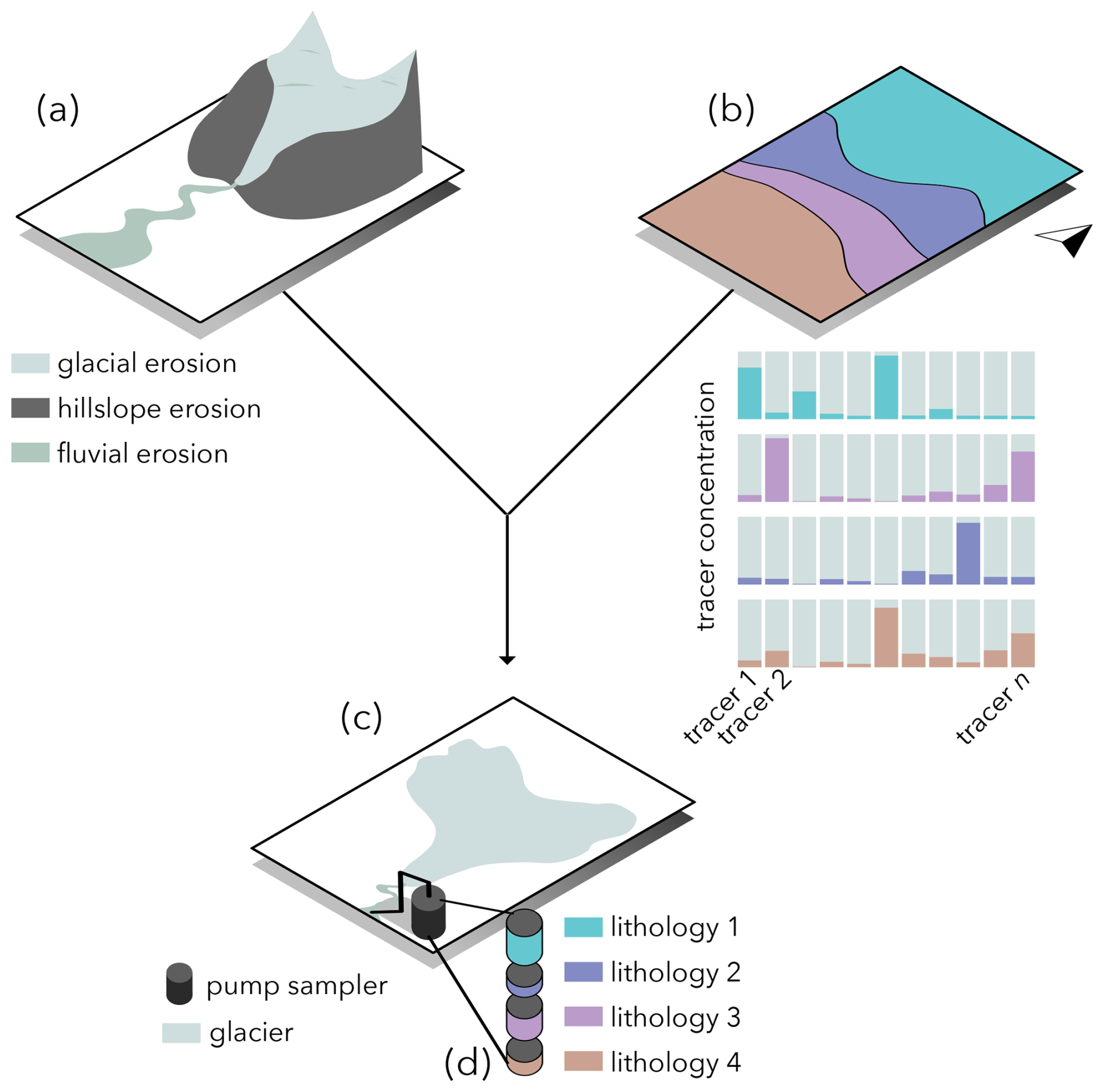
Figure 1 (a) Erosion processes active in a catchment, (b) geology and fingerprints of every lithology, (c) suspended sediment sampling at sink, with lithology proportions (d) reflecting the erosion rates in the different lithologies.

Formally, the forward statement reads:

$$\begin{array}{}\text{(1)}& d_i={\displaystyle \frac{{\sum }_{j=\mathrm{1}}^n{A}_{ij}\cdot \exp \left({\mathit{\epsilon }}_j\right)}{{\sum }_{j=\mathrm{1}}^n\exp \left({\mathit{\epsilon }}_j\right)}}\mathrm{for}i=\mathrm{1},\mathrm{\dots }m\end{array}$$

Where d_i is the tracer abundance of tracer mineral i in the suspended sediments, A_ij is the tracer abundance of tracer mineral i at source position j (pixel j), and the erosion rates are modelled in log-space: ${\mathit{\epsilon }}_j=\log \left(\frac{{\dot{e}}_j}{{\dot{e}}_{\mathrm{0}}}\right)$ with ${\dot{e}}_j$ being the erosion rate at pixel j and ${\dot{e}}_{\mathrm{0}}$ is a reference erosion rate (set to 1) to respect dimensional consistency. We cast the erosion rates in log-space to impose a positivity constraint, hence making this non-linear. Indeed, the linear version of this problem, as explained in De Doncker et al. (2020), sometimes yields negative values for $\dot{e}$, which we avoid here by solving for ε.

For simplicity, we redefine the data vector d as scaled by the total erosion rate:

$$\begin{array}{}\text{(2)}& \mathit{d}\leftarrow \mathit{d}\cdot \sum _j{\dot{e}}_j\end{array}$$

This allows us to rewrite the forward model in a simplified, dimensionless form:

$$\begin{array}{}\text{(3)}& \mathit{d}=\mathbf{A}\cdot \exp \left(\mathit{\epsilon }\right)\end{array}$$

where ${\dot{e}}_j={\dot{e}}_{\mathrm{0}}\cdot \exp \left({\mathit{\epsilon }}_j\right)$. In matrix form, the forward statement reads:

$$\begin{array}{}\text{(4)}& \left[\begin{array}{c}{d}_{\mathrm{1}}\\ \mathrm{⋮}\\ d_{\mathrm{m}}\end{array}\right]=\left[\begin{array}{cccc}{A}_{\mathrm{1},\mathrm{1}}& \mathrm{\cdots }& \mathrm{\cdots }& A_{\mathrm{1},n}\\ \mathrm{⋮}& & & \mathrm{⋮}\\ A_{m,\mathrm{1}}& \mathrm{\cdots }& \mathrm{\cdots }& A_{m,n}\end{array}\right]\cdot \exp \left(\begin{array}{c}{\mathit{\epsilon }}_{\mathrm{1}}\\ \mathrm{⋮}\\ \mathrm{⋮}\\ {\mathit{\epsilon }}_n\end{array}\right)\end{array}$$

2.2 Inverse model

To obtain the erosion rate map (Fig. 2a) that generated these sediments (Fig. 2b), we use an inversion method. By using the spatial distribution of the source areas (geological map) (Fig. 2c), we obtain an erosion rate map from the detrital data (fingerprint concentrations). In other words, we unmix the amalgamation of fingerprints in the detrital data, and the contribution of each source area in the detrital data equals the erosion rates.

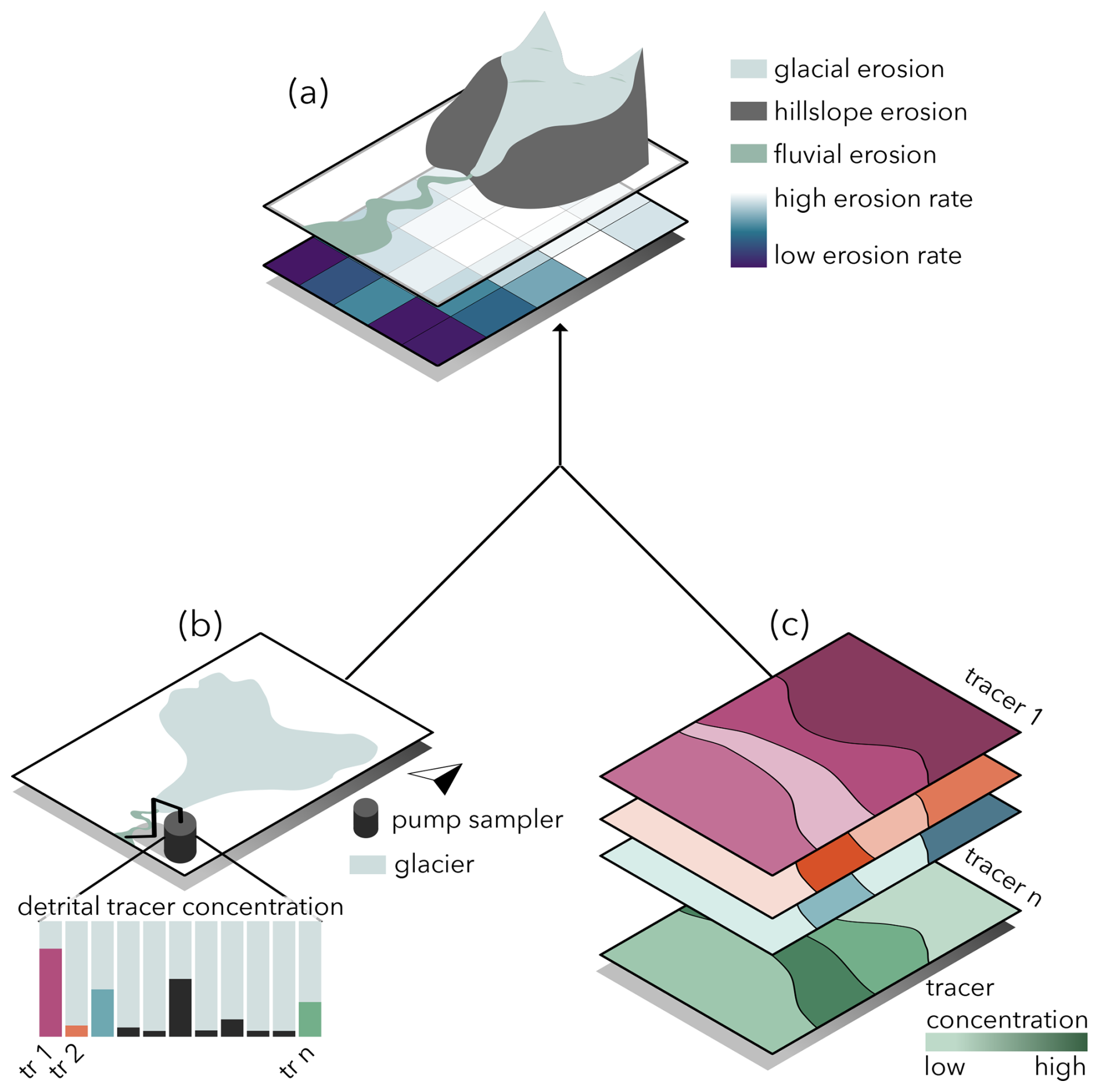
Figure 2 From detrital data and spatial information on tracer concentrations to an erosion rate map: (a) erosion rate map (raster) reflecting different erosion processes, (b) tracer concentrations in suspended sediments, (c) tracer concentration maps based on geology and lithological fingerprints.

Our inverse problem is underdetermined: the number of tracers, representing the data we have, is smaller than the number of pixels for which we want to infer the erosion rates. The solution is thus non-unique, meaning that many erosion rate maps could explain the data; mathematically, this means that our tracer matrix A is not invertible (it has more columns than rows). To deal with this, we implement a maximum a posteriori approach (MAP), where we seek the most probable erosion rate map given the observed detrital data and a prior knowledge (smoothness and expected magnitudes), following Bayes' theorem:

$$\begin{array}{}\text{(5)}& p\left({\mathit{\epsilon }}_{\mathrm{m}}|{\mathit{d}}_{\mathrm{obs}}\right)=p\left({\mathit{d}}_{\mathrm{obs}}|{\mathit{\epsilon }}_{\mathrm{m}}\right)\cdot {\displaystyle \frac{p\left({\mathit{\epsilon }}_{\mathrm{prior}}\right)}{p\left({\mathit{d}}_{\mathrm{obs}}\right)}}\end{array}$$

Where p(ε|d_obs) is the posterior, p(d_obs|ε_m) is the likelihood, and p(ε_prior) is the prior. To find the MAP estimate, we maximize the posterior, or equivalently, minimize the negative log-posterior for ε_m. We assume weak nonlinearity, where our forward model can be linearized around the prior, hence, the a posteriori probability density remains approximately Gaussian. Therefore, we can write the misfit function (ϕ(ε)) to be minimized as:

$$\begin{array}{}\text{(6)}& \mathit{\varphi }\left({\mathit{\epsilon }}_{\mathrm{m}}\right)=-\log \left(p\left({\mathit{d}}_{\mathrm{obs}}\right|{\mathit{\epsilon }}_{\mathrm{m}})\right)-\log \left(p\left({\mathit{\epsilon }}_{\mathrm{prior}}\right)\right)\end{array}$$

Which, in an approximately Gaussian setting, becomes (Tarantola, 2005):

$$\begin{array}{}\text{(7)}& \mathit{\varphi }\left({\mathit{\epsilon }}_{\mathrm{m}}\right)={\left(\mathit{d}\left({\mathit{\epsilon }}_{\mathrm{m}}\right)-{\mathit{d}}_{\mathrm{obs}}\right)}^{\mathrm{2}}\cdot {\mathbf{C}}_{\mathrm{d}}^{-\mathrm{1}}+{\left({\mathit{\epsilon }}_{\mathrm{m}}-{\mathit{\epsilon }}_{\mathrm{prior}}\right)}^{\mathrm{2}}\cdot {{\mathbf{C}}_{\mathrm{m}}}^{-\mathrm{1}}\end{array}$$

Where C_d and C_m are the data- and model covariance respectively, giving the data misfit ${\mathit{\varphi }}_{\mathrm{d}}\left({\mathit{\epsilon }}_{\mathrm{m}}\right)=({\mathit{d}}_{\mathit{\epsilon }}-{\mathit{d}}_{\mathrm{obs}}{)}^T{\mathbf{C}}_{\mathrm{d}}^{-\mathrm{1}}({\mathit{d}}_{\mathit{\epsilon }}-{\mathit{d}}_{\mathrm{obs}})$ and the prior misfit ${\mathit{\varphi }}_{\mathrm{prior}}\left({\mathit{\epsilon }}_{\mathrm{m}}\right)={\left(\mathit{\epsilon }-{\mathit{\epsilon }}_{\mathrm{prior}}\right)}^T{\mathbf{C}}_{\mathrm{m}}^{-\mathrm{1}}\left(\mathit{\epsilon }-{\mathit{\epsilon }}_{\mathrm{prior}}\right)$.

The data covariance is calculated as:

$$\begin{array}{}\text{(8)}& {\mathbf{C}}_{\mathrm{d}}={\mathit{\sigma }}_{\mathrm{d}}^{\mathrm{2}}\mathbf{I}\end{array}$$

with ${{\mathit{\sigma }}_{\mathrm{d}}}^{\mathrm{2}}$ as the data variance, and I the identity matrix.

The model covariance (controlling the variance around ε_prior) is computed as follows:

$$\begin{array}{}\text{(9)}& C_{\mathrm{m}}(i,j)={\mathit{\sigma }}_{\mathrm{m}}^{\mathrm{2}}\exp \left({\displaystyle \frac{s_{i,j}^{\mathrm{2}}}{L^{\mathrm{2}}}}\right)\end{array}$$

with ${{\mathit{\sigma }}_{\mathrm{m}}}^{\mathrm{2}}$ the prior variance, s_i,j the Euclidean distance between point i and j, and L the smoothing distance.

To minimize the misfit (Eq. 7), we compute the gradient of the misfit as

$$\begin{array}{}\text{(10)}& \mathrm{\nabla }\mathit{\varphi }\left(\mathit{\epsilon }\right)={\mathrm{\nabla }}_{\mathit{\epsilon }}{\mathit{\varphi }}_{\mathrm{d}}+{\mathrm{\nabla }}_{\mathit{\epsilon }}{\mathit{\varphi }}_{\mathrm{prior}}\end{array}$$

Since the gradient of the data misfit can be written as:

$$\begin{array}{}\text{(11)}& {\mathrm{\nabla }}_{\mathit{\epsilon }}{\mathit{\varphi }}_{\mathrm{d}}={\displaystyle \frac{\partial d_{\mathit{\epsilon }}}{\partial \mathit{\epsilon }}}\cdot {\displaystyle \frac{\partial {\mathit{\varphi }}_{\mathrm{d}}}{\partial d_{\mathit{\epsilon }}}}\end{array}$$

where the modelled data for model ε is written as ${\mathit{d}}_{\mathit{\epsilon }}=\mathbf{A}\cdot \exp \left(\mathit{\epsilon }\right)$, with the Jacobian G (showing how model predicted output changes with respect to the parameters) like:

$$\begin{array}{}\text{(12)}& {\displaystyle \frac{\partial d_{\mathit{\epsilon }}}{\partial \mathit{\epsilon }}}=\mathbf{G}=\mathbf{A}\cdot \exp \left(\mathit{\epsilon }\right)\end{array}$$

and:

$$\begin{array}{}\text{(13)}& {\displaystyle \frac{\partial {\mathit{\varphi }}_{\mathrm{d}}}{\partial d_{\mathit{\epsilon }}}}={\displaystyle \frac{\partial \left({\left({\mathit{d}}_{\mathit{\epsilon }}-{\mathit{d}}_{\mathrm{obs}}\right)}^{\mathrm{2}}{\mathbf{C}}_{\mathrm{d}}^{-\mathrm{1}}\right)}{\partial d_{\mathit{\epsilon }}}}\end{array}$$

plugging Eqs. (12) and (13) into Eq. (11), the gradient of the data misfit therefore is:

$$\begin{array}{}\text{(14)}& {\mathrm{\nabla }}_{\mathit{\epsilon }}{\mathit{\varphi }}_{\mathrm{d}}={\mathbf{GC}}_d^{-\mathrm{1}}\left({\mathit{d}}_{\mathit{\epsilon }}-{\mathit{d}}_{\mathrm{obs}}\right)\end{array}$$

and the gradient of the model misfit can be written as:

$$\begin{array}{}\text{(15)}& {\displaystyle \frac{\partial {\mathit{\varphi }}_{\mathrm{prior}}}{\partial \mathit{\epsilon }}}={\mathbf{C}}_{\mathrm{m}}^{-\mathrm{1}}\left(\mathit{\epsilon }-{\mathit{\epsilon }}_{\mathrm{prior}}\right)\end{array}$$

Combining Eqs. (14) and (15) in Eq. (10) so the total misfit gradient becomes:

$$\begin{array}{}\text{(16)}& \mathrm{\nabla }\mathit{\varphi }\left(\mathit{\epsilon }\right)={\mathbf{G}}^T{\mathbf{C}}_{\mathrm{d}}^{-\mathrm{1}}\left({\mathit{d}}_{\mathit{\epsilon }}-{\mathit{d}}_{\mathrm{obs}}\right)+{\mathbf{C}}_{\mathrm{m}}^{-\mathrm{1}}\left(\mathit{\epsilon }-{\mathit{\epsilon }}_{\mathrm{prior}}\right)\end{array}$$

Since our problem is non-linear, there is no analytical solution for the optimum of the misfit function, so a stepwise method is used:

$$\begin{array}{}\text{(17)}& {\mathit{\epsilon }}_{k+\mathrm{1}}={\mathit{\epsilon }}_k-\mathit{\mu }\mathrm{\nabla }\mathit{\varphi }\left(\mathit{\epsilon }\right)\end{array}$$

with μ being the step size, and ε_k+1 the posterior model after k+1 non-linear iteration steps.

To solve the non-linear inverse problem, we test and compare two iterative optimization approaches: (1) Steepest Descent (SD) and (2) the quasi-Newton (QN) method. Both rely on updating the model parameters (ε) iteratively to reduce the misfit between model and observed data, all the while not straying too far from the prior.

In the SD approach, the model update follows the direction of the gradient of the misfit (Eq. 16), preconditioned by the prior model covariance matrix C_m (Tarantola, 2005). The advantage of this method is that it does not require the resolution of a linear system at each iteration (Tarantola, 2005):

$$\begin{array}{}\text{(18)}& \begin{array}{rl}{\mathit{\epsilon }}_{n+\mathrm{1}}=& {\mathit{\epsilon }}_n-{\mathit{\mu }}_n\\ & \left({\mathbf{C}}_{\mathrm{m}}{\mathbf{G}}_n^T{\mathbf{C}}_{\mathrm{d}}^{-\mathrm{1}}\left({\mathit{d}}_n-{\mathit{d}}_{\mathrm{obs}}\right)+\left({\mathit{\epsilon }}_k-{\mathit{\epsilon }}_{\mathrm{prior}}\right)\right)\end{array}\end{array}$$

where G_n is the Jacobian at iteration n, C_m is the model covariance and μ_n is the step size.

In the QN approach, the misfit gradient (Eq. 16) is preconditioned using curvature information, with the Hessian (i.e. the second derivative of the misfit), leading to faster convergence (Tarantola, 2005):

$$\begin{array}{}\text{(19)}& \begin{array}{rl}{\mathit{\epsilon }}_{n+\mathrm{1}}=& {\mathit{\epsilon }}_n-{\mathit{\mu }}_n{\left({\mathbf{G}}_n^T{\mathbf{C}}_{\mathrm{d}}^{-\mathrm{1}}{\mathbf{G}}_n\right)}^{-\mathrm{1}}\\ & \left({\mathbf{G}}_n^T{\mathbf{C}}_{\mathrm{d}}^{-\mathrm{1}}\left({\mathit{d}}_n-{\mathit{d}}_{\mathrm{obs}}\right)+{\mathbf{C}}_{\mathrm{m}}^{-\mathrm{1}}\left({\mathit{\epsilon }}_k-{\mathit{\epsilon }}_{\mathrm{prior}}\right)\right)\end{array}\end{array}$$

2.3 Posterior uncertainty assessment

To estimate the uncertainty on our a posteriori erosion rate maps, different metrics can be used. The first one is the posterior covariance, where the square root of the diagonal can be interpreted as “uncertainty bars” on the erosion rates of the different pixels. Assuming an approximate Gaussian a posteriori probability density, the posterior covariance can be estimated by (Tarantola, 2005):

$$\begin{array}{}\text{(20)}& \stackrel{\mathrm{̃}}{{\mathbf{C}}_{\mathrm{m}}}\approx {\left(\left({\mathbf{G}}^T{\mathbf{C}}_{\mathrm{d}}^{-\mathrm{1}}\mathbf{G}\right)+{\mathbf{C}}_{\mathrm{m}}^{-\mathrm{1}}\right)}^{-\mathrm{1}}\end{array}$$

The posterior covariance is low where there is more certainty on the estimated erosion rates. The off-diagonal elements quantify correlations and trade-offs between pixels, with high absolute values indicating where the inversion cannot fully disentangle the sediment contributions of both pixels due to similar fingerprints, and low absolute values corresponding to two pixels with distinct fingerprints.

The second metric is the resolution, which shows how well the estimated erosion rate at a given pixel is resolved by the data, relative to the prior (Backus and Gilbert, 1968; Fox et al., 2014). If an exact solution existed for exact data (${\mathit{d}}_{\mathrm{exact}}=\mathbf{A}\cdot \exp \left({\mathit{\epsilon }}_{\mathrm{exact}}\right)$), the solution ($\stackrel{\mathrm{̃}}{\mathit{\epsilon }}$) would satisfy

$$\begin{array}{}\text{(21)}& \stackrel{\mathrm{̃}}{\mathit{\epsilon }}-{\mathit{\epsilon }}_{\mathrm{prior}}=\mathbf{R}\left({\mathit{\epsilon }}_{\mathrm{exact}}-{\mathit{\epsilon }}_{\mathrm{prior}}\right)\end{array}$$

So R is close to the identity operator I if we have perfectly resolved the “exact model”. The further R is from I, the less visible the parameters are in the data, in other words, the more diluted the signal is in the detrital data. Where the diagonal of R is close to 1, data have improved our knowledge considerately relative to the prior. The third metric is the ratio between the posterior model covariance and the “prior” model covariance. It shows how much more certain we are after an inversion, values closer to zero indicate a maximal variance reduction after the inversion (Tarantola, 2005):

$$\begin{array}{}\text{(22)}& {\stackrel{\mathrm{̃}}{\mathbf{C}}}_{\mathrm{m},\mathrm{norm}}={\displaystyle \frac{\sqrt{\stackrel{\mathrm{̃}}{{\mathbf{C}}_{\mathrm{m}}}}}{\sqrt{{\mathbf{C}}_{\mathrm{m}}}}}\end{array}$$

Furthermore, one must evaluate the data- and model misfit (Eq. 7). The data misfit explains how well the model – here: our a posteriori erosion rate map – explains the observed data. It is weighted by the data covariance, so low-uncertainty observations contribute more. A smaller data misfit indicates a good data fit. A higher data misfit implies poor model parameters or insufficient model flexibility, causing the model to fail to reproduce the observed data. We stop the non-linear iterations when the data-misfit stops decreasing, or when it exceeds the user-defined maximal allowed number of iterations.

The model misfit (Eq. 7) measures the deviation from the prior, weighed by the model covariance. Higher values indicate that the solution has evolved further away from the prior, whereas lower values appear with smoother or more regularised solutions. There is a well-known trade-off between data- and model misfit, as fitting the solution to the data makes it stray further away from the prior (Menke, 2012; Aster et al., 2013).

2.4 XRD data to fingerprints

To characterise the mineralogical fingerprints of both source and detrital samples, we employed X-ray diffraction (XRD) analysis. The steps that are described below can be applied to varying field sites, therefore, the descriptions are as general as possible. In Section 3.2, we demonstrate these by applying our method to the Gornergletscher catchment, Switzerland. In a first step, in-situ source samples are collected from every lithological unit across the study area (Fig. 3a and b). Note that multiple samples can be collected per source area, and the intra-source variance of the XRD signal can be propagated into the posterior solution by adding it in the data covariance matrix. Secondly, these samples are then powdered and analysed using XRD producing one diffractogram per sample (Fig. 3c). In these diffractograms, peaks represent constructive interference of X-rays incident at specific angles θ, indicating the presence of specific crystal structures. In a third step, the WinXRD Peak Finder algorithm corrects for baseline drift and removes the background noise, facilitating the identification of local maxima through thresholding and peak fitting. Fourth, to correct for instrumental or sample-related misalignments in peak position, the diffractograms are aligned to a pure quartz pattern (Butler et al., 2019). In a fifth step, diagnostic 2θ windows for each mineral are selected from RRUFF database reference spectra (Lafuente et al., 2016) (Fig. 3d and e). The diffraction peaks (and more specifically, the areas of these peaks) of our samples in these mineral-specific 2θ windows are indicative of mineral abundance. Sixth, to mitigate peak overlap, we average the total peak area within the 2θ windows corresponding to each mineral, rather than relying on individual peaks. At the end, these are normalized within each sample by dividing by the maximum observed peak area, yielding relative mineral concentrations on a scale from 0 to 1 (Fig. 3d and e). We can thereby derive the abundance of a given tracer t at pixel xy in A_t,xy as well as in the detrital data d_t (Eqs. 1–4). This approach allows for consistent comparison across both source and detrital samples while minimizing the influence of absolute intensity differences due to experimental and sample-related factors (Gjems, 1967; Weir et al., 1975; Bish and Post, 1989; Moore and Reynolds, 1990; Butler et al., 2019; Das et al., 2023, 2024).

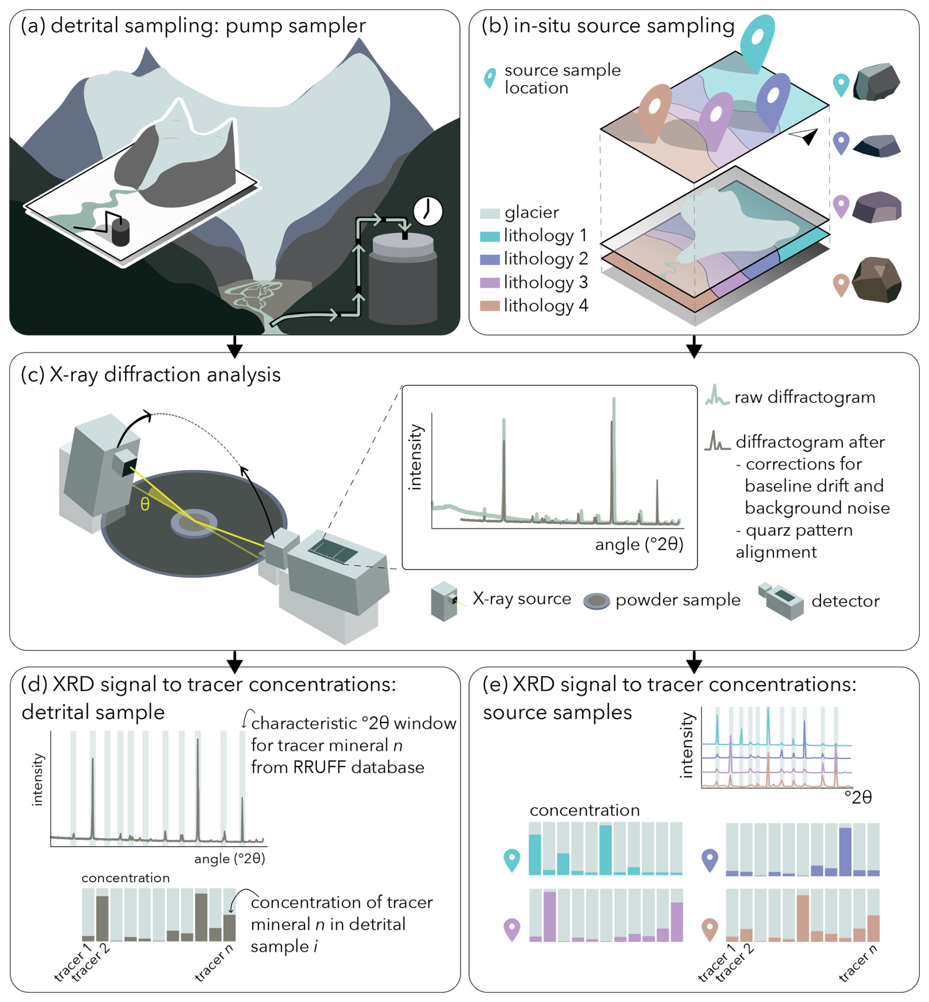
Figure 3 From samples to fingerprints: (a, b) sampling of sediments and of representative rock samples for the different source areas; (c) XRD analysis of powdered samples and corrections; (d, e) binning.

An important limitation of many sediment fingerprinting approaches is the dependence of tracer concentrations on grain size and post-depositional processes (D'Haen et al., 2012; Laceby et al., 2017; Collins et al., 2017). These issues are commonly referred to as grain-size effects, tracer fractionation, and source fertility problems (Garzanti et al., 2009). Specific concerns include (a) the production of new minerals through chemical weathering in the finest fraction of sediments and (b) lithology-dependent grain-size production, while suspended sediment samples predominantly capture fine particles. Three lines of evidence suggest that these effects are limited in our research setting.

First, the grain size of suspended sediment in the Gorner River was measured using laser diffraction (Malvern Mastersizer). The suspended sediment is dominated by silt-sized particles, with median grain sizes of 20–30 µm (d50 = 18–31 µm) and only a small clay fraction (< 2 µm) of 6 %–7 %. Most of the sediment therefore lies within the 2–63 µm silt fraction typical of glacially produced suspended sediment (“glacial flour”). These grain sizes indicate that the sediment is largely produced by physical comminution beneath the glacier rather than by chemical weathering.

Second, the mineralogical analysis focuses exclusively on primary rock-forming minerals (e.g., quartz, feldspars, pyroxenes, amphiboles, micas, serpentine minerals, garnet). Minerals that are typical products of chemical weathering (in this climatic setting: vermiculite, smectites or mixed layers in small amounts) were not included in the selected tracer minerals. The presence of chemically weathered minerals in the clay fraction is therefore unlikely to bias the fingerprinting results.

Third, we tested whether mineralogical signals vary with grain size by comparing pump-sampler samples with depth-integrated samples collected at the same site. Pump samplers collect sediment at a fixed height within the water column and therefore tend to sample a narrower grain-size range, whereas depth-integrated samples capture a broader grain-size distribution. If mineral abundances were strongly grain-size dependent, we would expect large differences between these two sampling methods. However, the mineralogical signals are very similar between the pump and depth-integrated samples, suggesting that grain-size dependent mineralogical fractionation is limited in this dataset.

3 Validation

We validate our XRD-based inversion method on the Gornergletscher catchment, a site well-suited for this study due to the availability of multi-year suspended sediment datasets and the presence of strongly heterogeneous bedrock lithologies (Fig. 4).

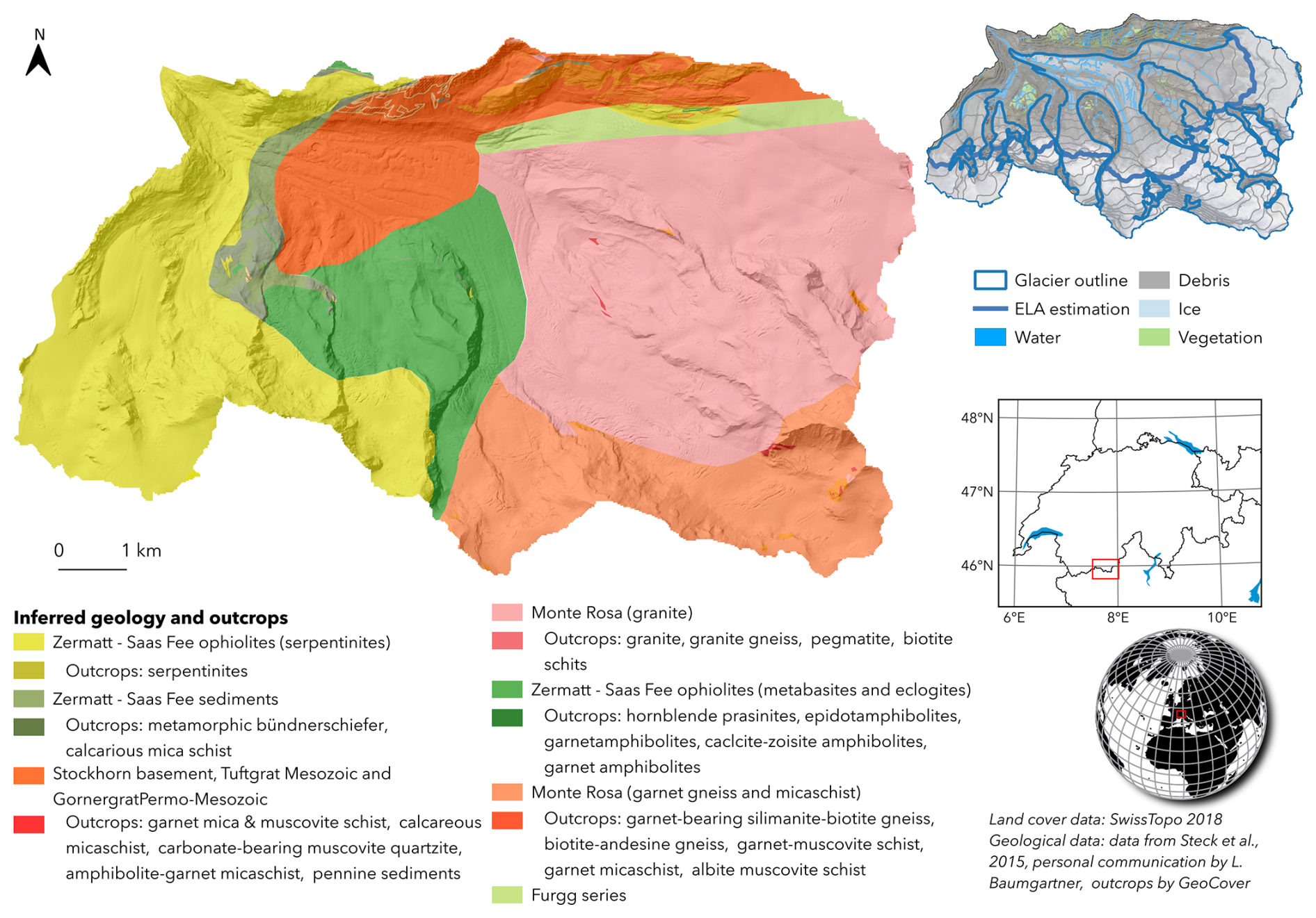
Figure 4 Study area: location, land cover and geology.

Figure 4 shows the study area, with the inferred geology, outcrops and land cover. In ice-covered regions, where direct geological mapping is not possible, we infer the lithology based on regional geological knowledge. This interpretation is informed by lithological observations at ice-free outcrops (Bearth, 1953; Steck et al., 2015). The Gornergletscher catchment contains a diverse set of lithologies derived from both oceanic and continental domains of the Pennine Alps. The Zermatt–Saas Fee ophiolites include serpentinites (predominantly antigorite and chrysotile), metabasites, and eclogites, while Penninic Mesozoic sedimentary units (Bündnerschiefer) consist mainly of calcareous mica schists and quartzites. The Monte Rosa nappe comprises coarse-grained granites, granite gneisses, and garnet-mica schists. The Stockhorn, Tuftgrat, and Gornergrat units are dominated by amphibolite-bearing garnet-mica schists and related metamorphic rocks. The Furgg series comprises a mixed association of ophiolites, meta-arkoses, quartzites, marbles, amphibolites, and leucocratic gneisses (Bearth, 1953; Steck et al., 2015).

Starting with synthetic tests, from fully synthetic source- and detrital data, we evaluate the different inversion schemes, assess the impact of data degradation, and investigate the sensitivity to various hyperparameters. We then apply the inversion to natural data of the Gornergletscher, (1) to investigate whether the inferred XRD source fingerprints align with the expected mineralogical compositions of the lithologies, (2) to test if sediment samples from a subcatchment are attributed only to lithologies present within the subcatchment boundaries, (3) to assess how the incorporation of XRD-based fingerprints alongside zircon data improves the stability and accuracy of the posterior solution.

3.1 Synthetic tests

3.1.1 Forward-inverse tests: Quasi-Newton approach

To validate our inversion model, we generate synthetic detrital data using the forward model applied to a “true” erosion rate map featuring a localised hotspot with elevated erosion intensities (Fig. 5a). The synthetic data are then used as input for the non-linear inversion. After several iterations, the inversion yields an a posteriori erosion rate map (Fig. 5b), which we compare to the original “true” map. This comparison enables us to assess the accuracy and robustness of the inversion procedure with a given dataset (Fig. 5c).

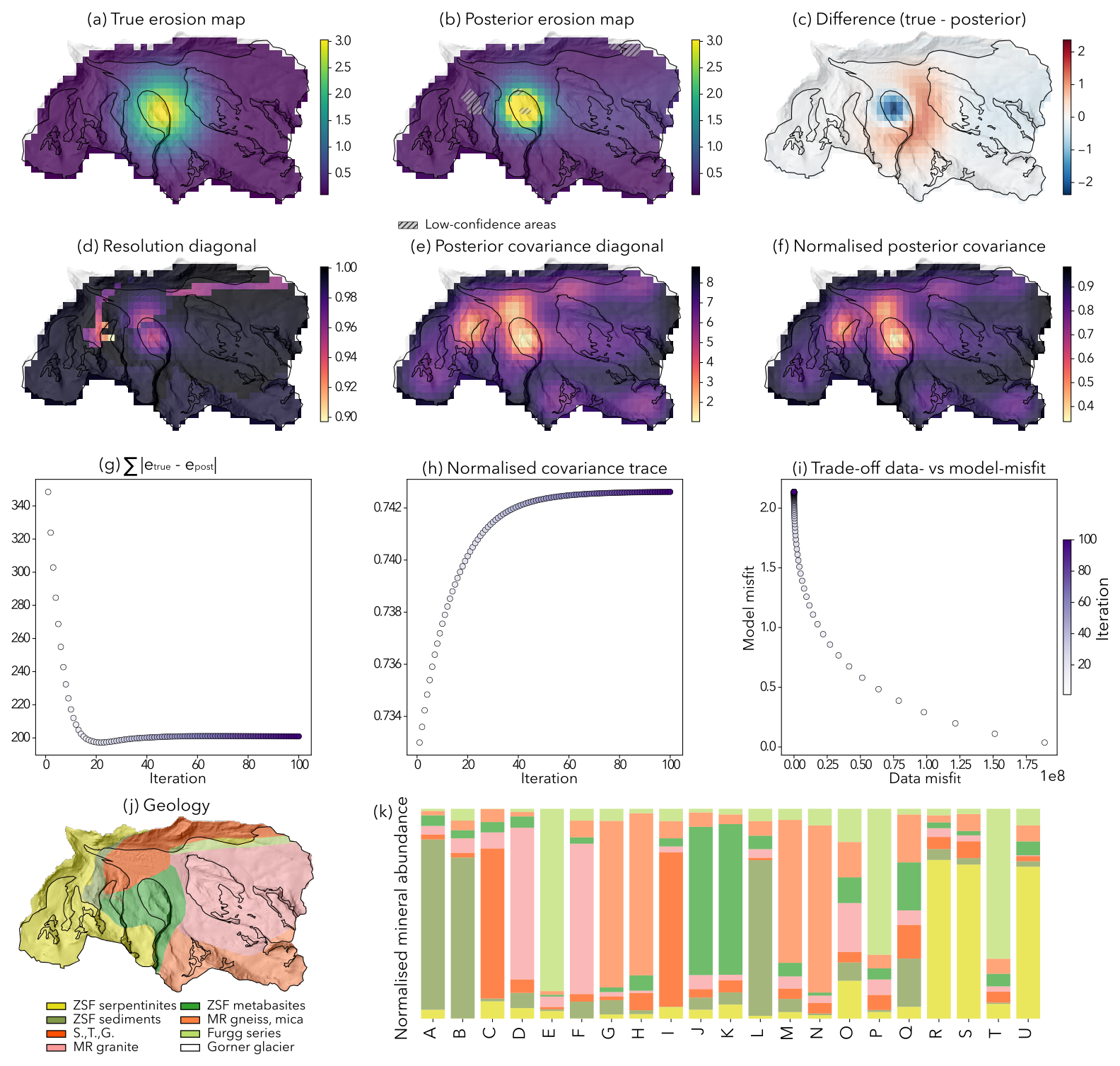
Figure 5 Results of the Quasi-Newton approach: (a) “true” erosion map, (b) posterior erosion map, (c) difference between “true” and posterior erosion map, (d) resolution diagonal, (e) posterior covariance diagonal, (f) normalised posterior covariance, (g) sum of difference between “true” and posterior erosion map during non-linear iterations, (h) normalised posterior covariance during non-linear iterations, (i) trade-off between data- and model misfit during non-linear iterations, (j) geological map, (k) synthetic source tracer concentrations.

In a first test, we use the QN approach with 100 iterations, the full tracer mineral information from synthetic source fingerprints (Fig. 5k), a smoothing distance of 4 times the pixel size (L=1200 m), a model standard deviation of 3 (dimensionless, as epsilon is dimensionless), a data standard deviation of 0.01 mm yr⁻¹ and a prior equal to the average true erosion rate.

The quasi-Newton (QN) approach generates a posterior erosion rate map that closely matches the true erosion pattern, both in spatial distribution and magnitude (Fig. 5b). The primary differences occur within larger lithological units, where reduced spatial variability in tracer concentrations limits the model's resolving power (Fig. 5c).

Small lithological units (such as Zermatt Saas-Fee sediments and Furgg series (Fig. 4) and Fig. 5j) may be under-represented in the mixing process, making their signals harder to distinguish, leading to lower resolution (Fig. 5d). Posterior covariance is lowest in regions of high erosion, where the signal is strongest and most easily inferred (Fig. 5e). Moreover, uncertainty tends to be lower at boundaries between lithological units, where greater spatial variability in tracer concentrations enhances model sensitivity. The same pattern is visible in the normalised posterior variance, with lower values indicating better constraint (Fig. 5f).

Over the course of the non-linear iterations, the difference between the true and posterior erosion rates initially decreases rapidly, then plateaus (Fig. 5g). The posterior covariance follows a similar trend: it rises steeply in early iterations before levelling off (Fig. 5h). The trade-off curve reflects the model's “greedy” optimisation strategy: initially minimising the data misfit, with the prior term gradually constraining the solution to prevent over-fitting (Fig. 5i).

3.1.2 Forward-inverse tests: steepest descent approach

In the next test, we use the synthetic data as input for the inversion model, this time using the steepest descent approach in the inversion method.

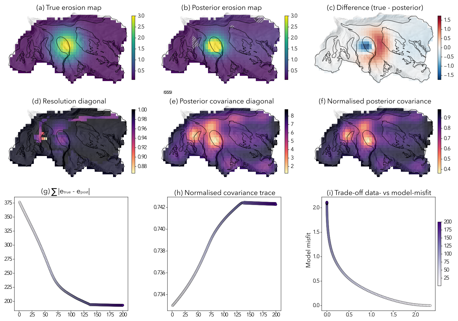
Figure 6 Results of the Steepest-Descent (SD) approach: (a) “true” erosion map, (b) posterior erosion map, (c) difference between “true” and posterior erosion map, (d) resolution diagonal, (e) posterior covariance diagonal, (f) normalised posterior covariance, (g) sum of difference between “true” and posterior erosion map during non-linear iterations, (h) normalised posterior covariance during non-linear iterations, (i) trade-off between data- and model misfit during non-linear iterations.

In initial experiments, the steepest descent approach proved unstable, requiring the normalization of the gradient. While this stabilization prevents divergence, it also forces each iteration to take steps of similar magnitude regardless of the actual gradient size. As a result, sharp features and narrow peaks in the posterior erosion rate distribution are smoothed out or missed (Fig. 6c), and more iterations are needed to converge to a posterior result as close to the true erosion rate map as the QN posterior (Fig. 5). This limited sensitivity to strong gradients also leads to oscillations in the posterior covariance, visible after 125 iterations, as the Jacobian fluctuates between iterations (Fig. 5g versus Fig. 6g). Nevertheless, the spatial patterns of uncertainty remain consistent, with lower posterior uncertainty in regions of high erosion rates and along boundaries between lithological units (Fig. 6d, e and f).

Based on these findings, we adopt the Quasi-Newton (QN) approach for all subsequent tests, as it provides a more stable and accurate reconstruction of the erosion rate patterns. The quasi-Newton scheme was also tested using a more complex synthetic erosion rate map; the results of this experiment are presented in Appendix A.

3.1.3 Data degradation tests

We assess the sensitivity of the inversion model to data degradation through three scenarios, each designed to reflect a common source of uncertainty in sediment provenance studies. These sensitivity tests are run with 25 iterations, a smoothing distance of 4 times the pixel size (L=1200 m), a model standard deviation of 3, a data standard deviation of 0.01 mm yr⁻¹, a prior equal to the average true erosion rate, and a step size μ of 0.1. For the detailed erosion rate map results, we refer to Appendix B.

In the first scenario, we test the impact of geological map uncertainty, using different geological maps to generate the synthetic data and to perform the inversion. Hence, the effect of uncertainty in subsurface geology is simulated, which is especially relevant in glacierized regions where direct observation of lithology is limited. The difference in lithological coverage between the two maps used as forward and inverse input is quantified by area mismatch (expressed in m²) between the lithological unit boundaries of the original geological map and those of the modified map.

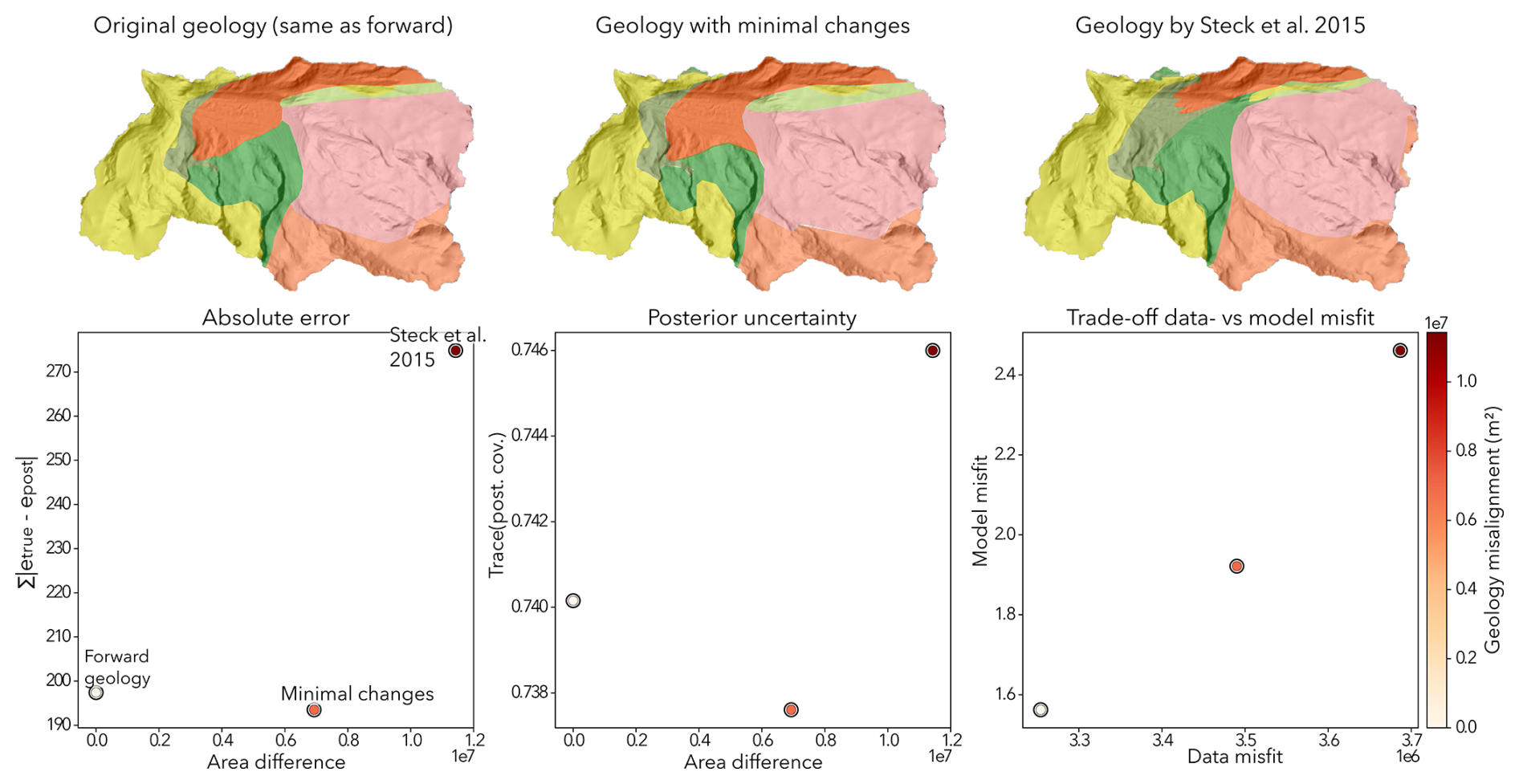
Figure 7 Scenario 1: geological map uncertainty (the colour on the scatterplot indicates area difference (m²) between the lithological map used to generate the synthetic data and the one used in the inversion). In the left scatterplot, the labels correspond to the maps above.

Three geological cases are investigated: (1) using the same geological map in the forward and inverse method, (2) using a geological map with minimal difference from the one used to generate the detrital data, (3) the map proposed by (Steck et al., 2015) with the biggest area mismatch. In Fig. 7, the three geological maps are visualized, as well as their impact on the absolute error, the normalized posterior uncertainty, and the trade-off between data- and model misfit. The area mismatch is colour coded in the scatterplots.

We observe that the greater the mismatch between the geological map used in the inversion and the one used to generate the synthetic data, the larger the discrepancy between the posterior and true erosion rate maps. Surprisingly, a simplified geological map with minimal changes from the truth results in a more accurate posterior erosion map than the original geological map itself. This occurs because the adjustments in the inversion map shift the centre of the Zermatt–Saas-Fee ophiolites (metabasites and eclogites) unit closer to the centre of the true erosion-rate bump. However, in all cases, both data misfit and model misfit increase as map uncertainty grows.

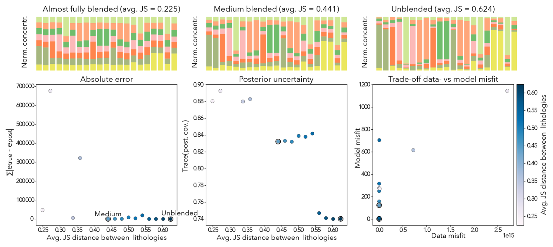
Figure 8 Scenario 2: blended fingerprints. In the top row, 3 examples are given, first the most blended source signatures, then the half-way in between source signatures, and then the original synthetic fingerprints. These three examples are labelled in the left scatterplot and indicated with thick black circles on the other scatterplots. Note that the most blended example did not have a stable solution and is therefore not plotted.

In the second scenario, with blended source fingerprints, we progressively homogenize the source fingerprints by approaching each lithology's mineral concentration to its mean across all lithologies. This reduces the distinctiveness between sources, which is quantified using the average Jensen-Shannon (JS) distance, which measures the similarity between two probability distributions. Values closer to zero indicate more similar (less distinguishable) source signatures. We compute the JS distance between all pairs of source XRD signatures and use the average across all combinations. Figure 8 illustrates three fingerprint sets: (1) highly blended, (2) intermediate, and (3) the original synthetic fingerprints. In total, 20 values between the highly blended and the original synthetic fingerprints are tested, with their average JS distance colour-coded in the scatterplots that show the impact on the posterior solution.

The more resemblant the source fingerprints are, the more difficult it is to find a coherent posterior solution. As the JS distance decreases below 0.55, both absolute error and posterior uncertainty rise sharply, with errors exceeding 700 mm yr⁻¹ for JS < 0.44. In many of these cases, the inversion fails to converge to a stable posterior solution. This indicates that poorly distinguishable fingerprints are a major limitation in source attribution.

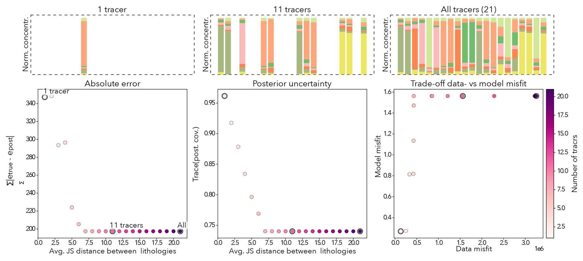
Figure 9 Scenario 3: reduced number of tracer minerals. In the top row, 3 examples are given, first the source signature using only one tracer mineral, then using 11 tracer minerals, and then the original synthetic fingerprints with the full set of tracer minerals. These three examples are labelled in the left scatterplot and indicated with thick black circles on the other scatterplots.

In the third scenario, we investigate the effect of reducing the number of tracer minerals. We perform a Principal Component Analysis (PCA) to retain the subset of tracers that explain the maximum variance in the mineralogical fingerprints. Figure 9 shows the source fingerprints of three configurations: (1) a single tracer, (2) the top 11 tracers, and (3) the full tracer set. In total, the full range between 1 and 21 tracers is tested, with colour-coded scatterplots showing the impact of the tracer count reduction on the posterior solution.

The inversion with 7 tracers results in approximately the same posterior solution as with the full tracer set. However, when the number of tracers drops below 7, the absolute error increases rapidly, as does the posterior uncertainty, while the data misfit and model misfit drop.

To summarize, among the three tested scenarios, the strongest impact on the posterior solution arises from reduced fingerprint distinctiveness. Geological map uncertainty follows as the second most influential factor. In contrast, reducing the number of tracers has a comparatively limited effect – provided that the most informative ones are retained.

3.1.4 Parameter sensitivity tests

Next, we assess the sensitivity of the inversion to key model parameters. Specifically, we test the impact of (1) the model standard deviation, which controls how far the posterior can deviate from the prior, (2) the smoothing distance used in the model covariance, (3) the data standard deviation, (4) the step size of the non-linear iterations, which controls the magnitude of the updates, and (5) the maximal amount of non-linear iterations during the inversion process. The results of the hyperparameter sweeps are shown in Fig. 10.

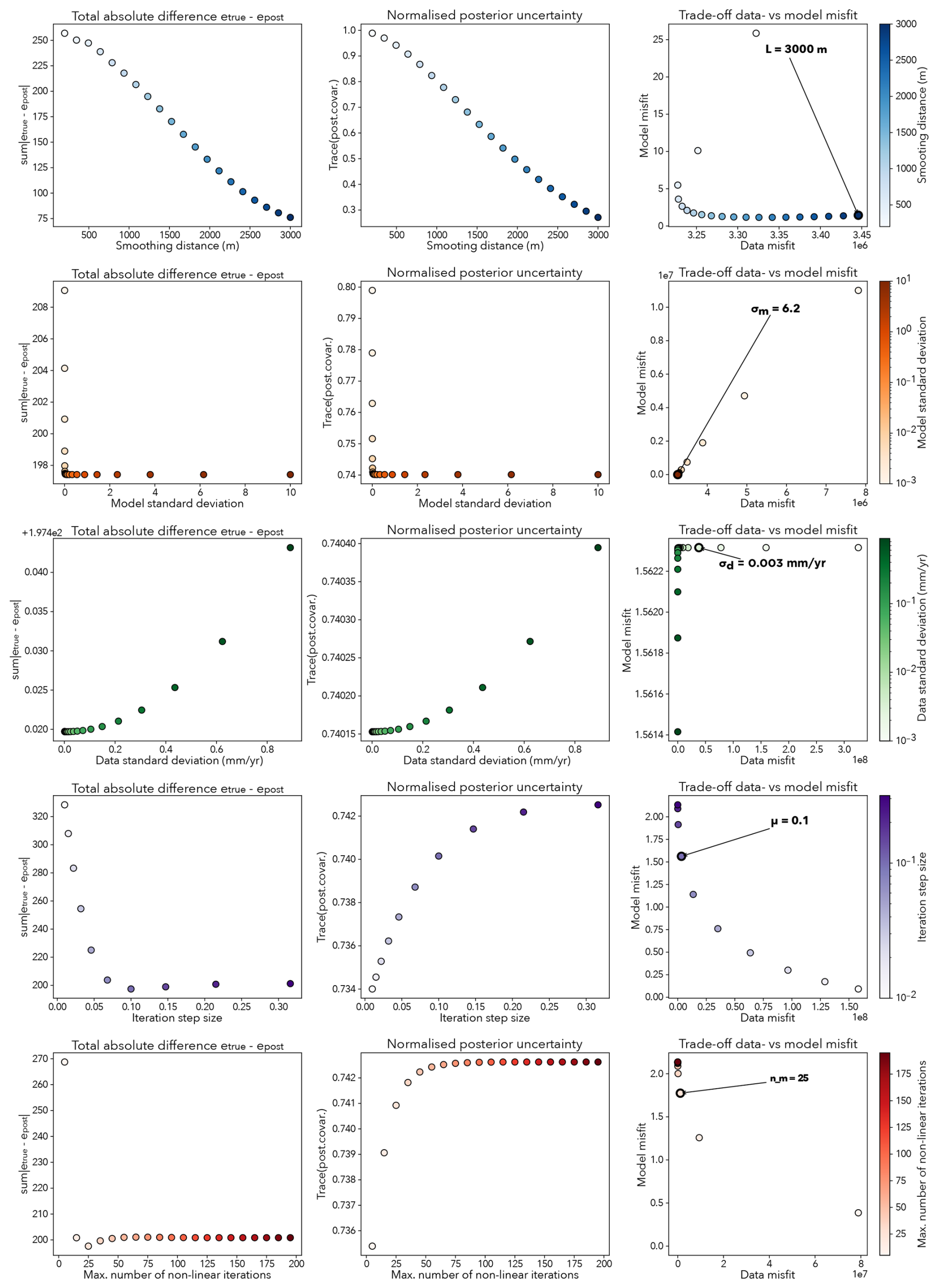
Figure 10 Results of parameter sweeps: first column: total absolute difference between true and posterior erosion rate maps, second column: normalised posterior uncertainty, third column: trade-off between data- and model-misfit for different parameter values. First row: smoothing distance L, second row: model standard deviation σ_m, third row: data standard deviation σ_d, fourth row: step size μ, fifth row: maximal number of non-linear iterations n_m.

As the smoothing distance increases, the posterior solution generally approaches the true erosion rate map, and overall uncertainty decreases. However, beyond approximately 10 times the pixel size (3000 m), the solution becomes overly smooth, causing the posterior to deviate from the true erosion rates. A longer smoothing distance effectively constrains the posterior closer to the prior (set here as the average true erosion rate) resulting in a reduced difference between posterior and true values, decreased model misfit, but increased data misfit.

Increasing the model standard deviation allows the inversion more freedom to diverge from the prior, improving data fit and reducing the difference between posterior and true erosion rates. Low model standard deviation values produce both high data and model misfits.

Very low data standard deviation values lead to large differences between the posterior and true erosion rate maps, likely due to overfitting or unstable gradients. As data standard deviation increases, the absolute difference first decreases to a minimum, then rises to a plateau at higher values. At very low data standard deviation, both data and model misfits are high; with increasing data standard deviation, model misfit remains high while data misfit decreases sharply. Beyond a data standard deviation of approximately 10–2 mm yr⁻¹, model misfit begins to decrease rapidly while data misfit stabilizes.

The optimal non-linear step size is 0.1; smaller values limit the evolution of the posterior from the prior, preventing convergence towards the true erosion map, as shown in the trade-off between data- and model misfit.

Only when the maximum number of non-linear steps is reduced below 25 does the posterior fail to converge to the true erosion map. Beyond 115 iterations, the change in data misfit between successive steps falls below 10⁻⁵, indicating that posterior solutions evolve only minimally after the 115th iteration.

3.2 Natural data tests

To evaluate our inversion framework, we use real X-ray diffraction (XRD) mineralogical fingerprints obtained from bedrock samples corresponding to the main lithological units of the Gornergletscher catchment. These measured fingerprints serve as the source signatures. To obtain the mineralogical fingerprints, we focused on a set of 21 minerals expected to be characteristic of the main lithologies in the catchment, including: Tremolite, Talc, Quartz, Pyroxene, Phlogopite, Paragonite, Omphacite, Muscovite, Microcline, Magnesite, Glaucophane, Fayalite, Dolomite, Diopside, Chrysolite, Antigorite, Anorthite, Annite, Ankerite, Almandine, and Albite. We powdered the source samples and processed the resulting XRD data using the Peak Finder algorithm and quartz peak alignment. By extracting the relative peak areas within diagnostic 2θ windows for each of the 21 target minerals, we obtained the mineral concentrations characterizing each lithological unit (Fig. 11). For the Monte Rosa (granite) unit, four samples have been collected (two sand samples and two rock samples that were crushed before XRD analysis); for the Zermatt Saas Fee ophiolites (metabasites, eclogites) unit, one sand and one rock sample have been collected; for all other units, a single sample is used. The error bars in Fig. 11 represent the inter-sample variability for these two units. Forward–inverse tests indicate that this variability remains sufficiently low to allow recovery of the true erosion pattern when this uncertainty is propagated via the data covariance matrix (C_d) as tracer-specific standard deviations. In this case, the misfit $\sum |e_{\mathrm{true}}-e_{\mathrm{post}}|$ ranges between 260 and 330 mm yr⁻¹ when using single-sample fingerprints in the inversion and inter-sample averages in the forward model, compared to 210 mm yr⁻¹ when inter-sample averages are used consistently in both forward and inverse models.

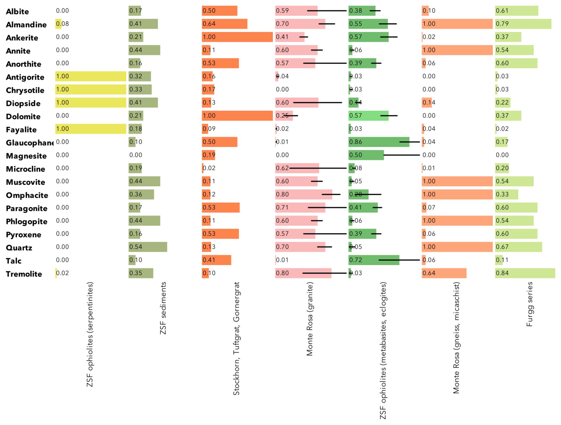
Figure 11 Normalised XRD-based mineralogical fingerprints of the different source areas of the Gornergletscher catchment. From left to right: ZSF ophiolites (serpentinites), ZSF sediments, Stockhorn-Turftgrat-Gornergrat, Monte Rosa (granite), ZSF ophiolites (metabasites, ecologites), Monte Rosa (gneiss, micaschist), Furgg series. Errorbars indicate the variability of the mineralogical signal between different samples for the same lithological unit.

The mineralogical fingerprints derived from processed and binned XRD data align well with established knowledge of the lithology in the Gornergletscher catchment (Bearth, 1953; Steck et al., 2015), supporting the (1) the robustness of the cleaning and binning approach, and (2) the validity of the input data for the inversion method. Bearth (1953) and Steck et al. (2015) further indicate that the Zermatt Saas-Free ophiolites (metabasites & eclogites) potentially have the strongest internal mineral variability, due to the unit spanning different metamorphic facies, as confirmed in Fig. 11.

3.2.1 Natural known mixture experiment

To evaluate the robustness of using XRD-based mineralogical fingerprints, we apply our inversion model to real sediment samples. Typically, the reliability of a given fingerprinting method is tested using known mixture experiments, where source materials are combined in predefined proportions and the unmixing method is assessed based on its ability to recover those proportions. Here, we use a natural analogue of that test. We collected sediment samples at the Gorner-Grenzgletscher confluence, with a catchment draining only the north-eastern portion of the study catchment. These samples are used as input for the inversion model, while the tracer matrix A is constructed using the geological map of the entire catchment. In other words, the model is not constrained to the contributing sub-catchment and is free to attribute the detrital signal to any lithology in the full domain. If the XRD fingerprinting method is robust, the inversion should attribute erosion only to lithologies present within the sub-catchment. Only the Zermatt–Saas Fee sediment unit does not have outcrops in the Gorner-Grenz subcatchment (Steck et al., 2015), as shown in Fig. 12.

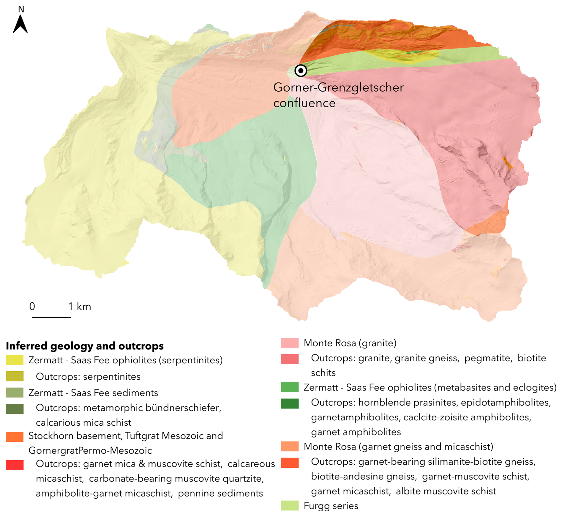
Figure 12 Lithology and outcrops in the Gorner-Grenz confluence subcatchment. The only unit not having outcrops in the subcatchment is the Zermatt–Saas Fee sediments unit.

Merging the inversion results from multiple detrital samples collected at the sink of this sub-catchment shows that the predicted erosion rates for pixels within the Zermatt–Saas Fee unit (ZSF sediments) are close to zero (Fig. 13). Some spillover occurs from adjacent lithologies, but the overall pattern confirms that the inversion respects geological boundaries when the XRD fingerprints provide sufficiently distinct signals.

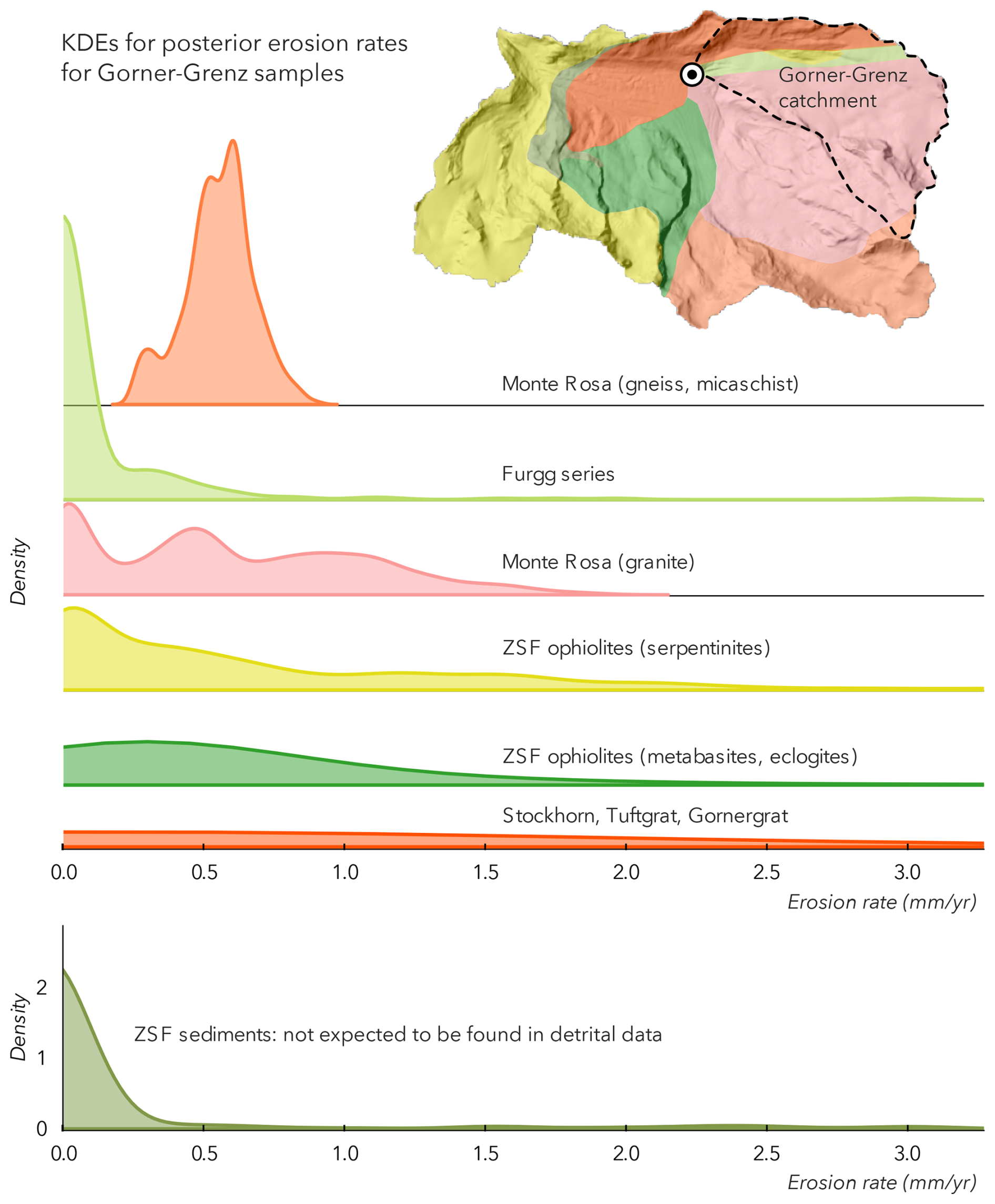
Figure 13 Kernel density estimates (KDE) of predicted erosion rates for all pixels within each lithological unit, based on multiple inversions using detrital samples from the Gorner–Grenz confluence subcatchment. For each lithology, the KDE integrates results from all inversions to show the distribution of predicted erosion rates. A rightward shift of the KDE peak indicates generally higher predicted erosion rates for that lithology; a taller peak indicates greater consistency across inversions.

In other words, the model correctly attributes the sediment data from the subcatchment to the lithologies present within the subcatchment and it does not attribute it to the Zermatt Saas-Fee sediments unit which is not present in the subcatchment.

This natural case study supports the reliability of our XRD fingerprinting approach in constraining erosion sources, even in complex glacial catchments.

3.2.2 Zircon comparison

To benchmark the performance of our XRD-based fingerprinting method, we compare it against a zircon-based fingerprinting approach applied to the same detrital sample. It highlights the strengths and limitations of each fingerprinting method and illustrates how combining complementary datasets can improve the inversion outcome.

Zircon grains were extracted and U-Pb dated from both the source lithologies and the detrital sample collected on 28 June 2019, at 13:30 CEST/UTC+2, following the methodology described in Belotti (2021). Using the approach outlined in De Doncker et al. (2020), we derived mineralogical fingerprints based on distinct age-concentration distributions of zircon populations.

We applied the inversion method to the zircon detrital data using the following parameters: QN scheme, 25 iterations, a smoothing distance of 4 times the pixel size (L=1200 m), a model standard deviation of 3 (dimensionless), a data standard deviation of 0.01 mm yr⁻¹, a prior equal to the average true erosion rate, and a step size μ of 0.1. The resulting posterior erosion rate map is shown in Fig. 14.

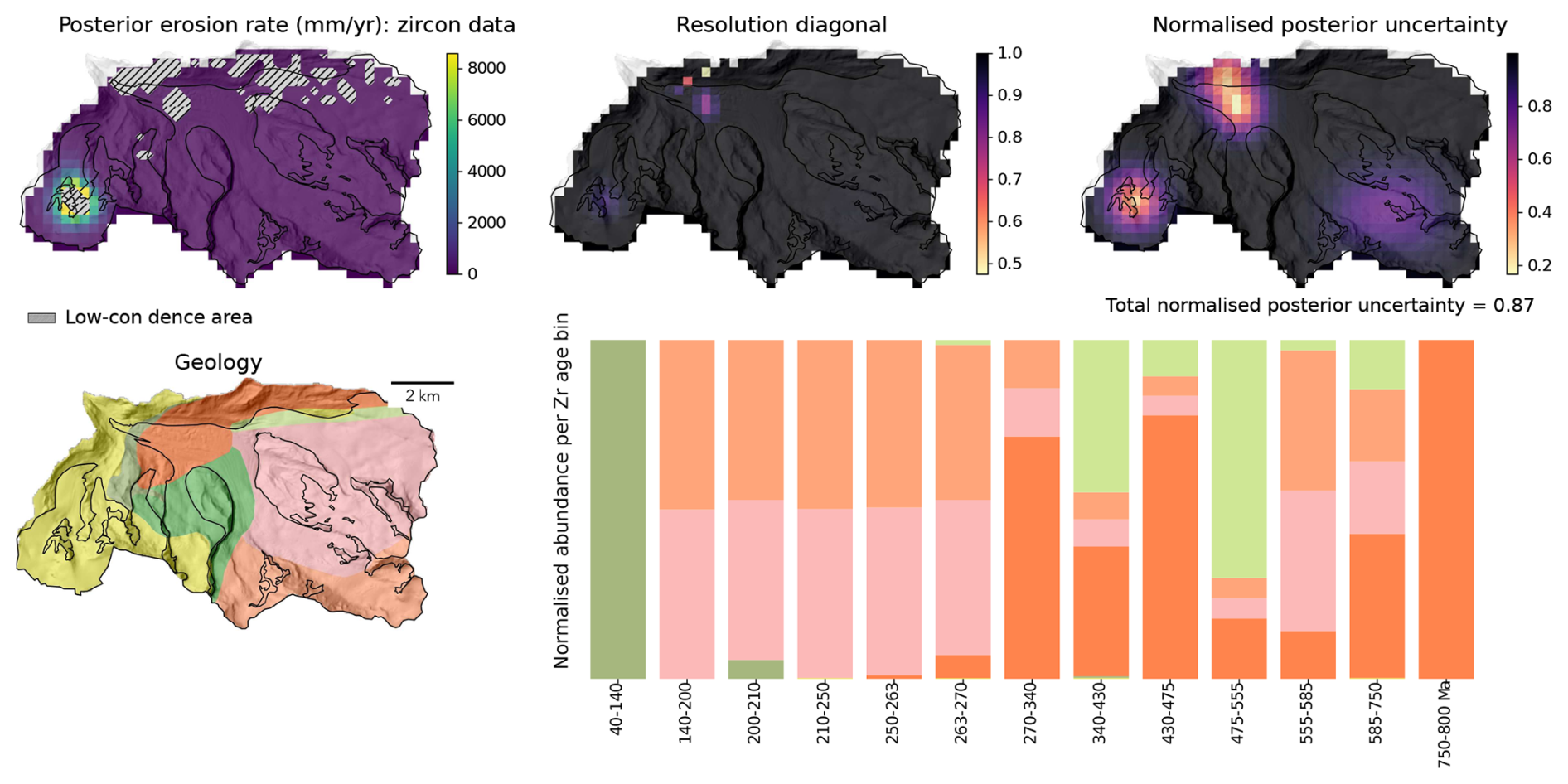
Figure 14 Posterior erosion rate map using Zr fingerprint data, the resolution for the posterior, the normalized posterior uncertainty, the geological map and the source fingerprints.

As shown in the source signatures in Fig. 14, zircon data were not available for two lithological units: no zircon grains were recovered from the Zermatt–Saas Fee (ZSF) ophiolites (metabasites and eclogites), and no age data were available for the Monte Rosa garnet–gneiss (MR g–g) unit. Moreover, the Zermatt–Saas Fee ophiolites (serpentinites) contain only very low concentrations of zircons. To compensate for the lack of age data for the MR g–g unit, we assigned the MR g–g unit the same zircon-age fingerprint as the Monte Rosa granite unit.

Despite these adjustments, the resulting posterior solution is highly unstable, with extreme erosion rate values (>8000 mm yr⁻¹), low resolution, and a high total normalized uncertainty $\left(\frac{\mathrm{tr}\left(C_{\mathrm{m},\mathrm{post}}\right)}{\mathrm{tr}\left(C_{\mathrm{m}}\right)}\right)$ value of 0.87.

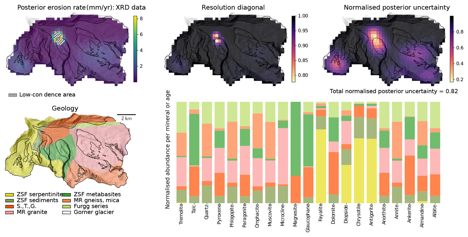
Figure 15 Posterior erosion rate map using XRD fingerprint data, the resolution for the posterior, the normalized posterior uncertainty, the geological map, and the source fingerprints.

We then applied the same nonlinear inversion technique to the XRD-derived dataset acquired from a detrital sample taken at the same date and time. The results are shown in Fig. 15.

Compared to the zircon-only results, the XRD-based posterior shows greater stability. While both datasets indicate sediment source activation in the serpentinite-rich region in the southwest, the XRD solution identifies the main erosion peak in the center of the domain and a secondary peak in the Monte Rosa granite area. The normalized posterior uncertainty is slightly lower at 0.82.

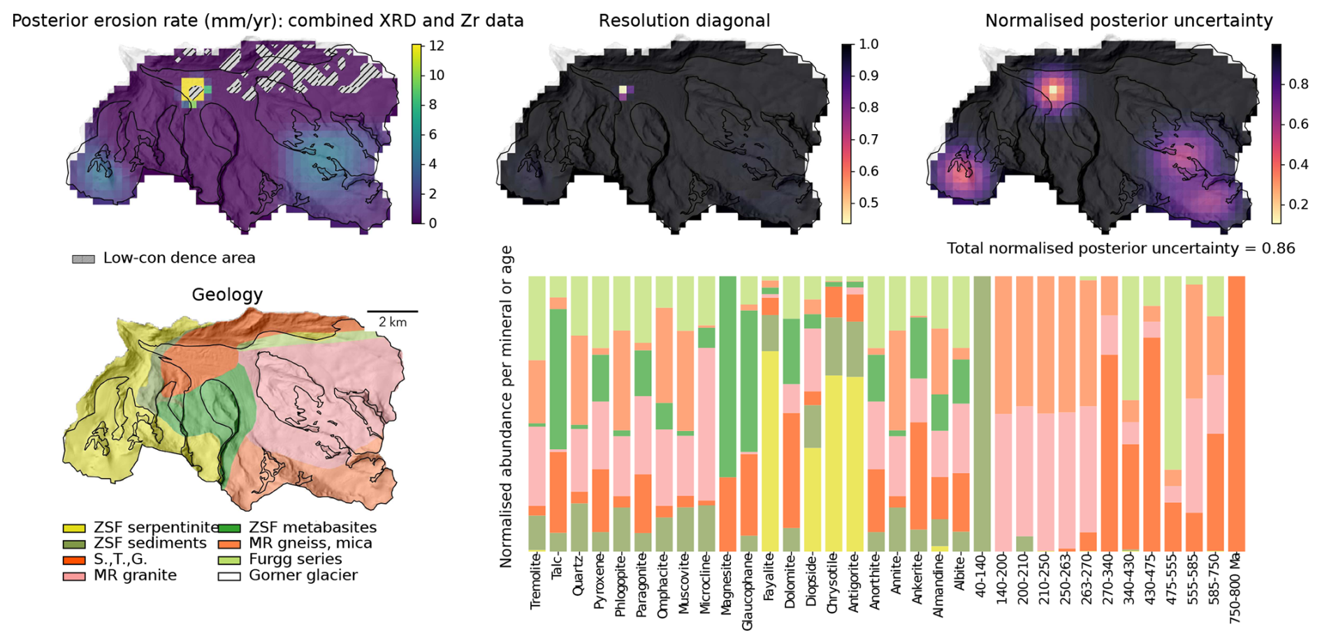
Figure 16 Posterior erosion rate map using a combination of zircon-age and XRD fingerprint data, the resolution for the posterior, the normalized posterior uncertainty, the geological map, and the source fingerprints.

Finally, we combine both zircon and XRD data by concatenating the tracer concentration matrices A of the zircon and XRD approaches, as well as both corresponding detrital data vectors. We run the inversion method with the same inversion parameters on this concatenated dataset, with the results shown in Fig. 16.

Adding XRD data to the zircon dataset stabilizes the inversion and improves the posterior solution. The normalized posterior uncertainty decreases slightly to 0.86 (from 0.87 in the zircon-only case), and the average Jensen-Shannon distance between source fingerprints increases from 0.48 to 0.57, indicating improved distinguishability. The resulting erosion pattern more closely resembles the XRD-only solution but benefits from the complementary information contained in the zircon fingerprints.

4 Discussion

We explained and validated the use of binned XRD peak-area data as mineralogical fingerprints within a non-linear inversion scheme to infer erosion rate maps. The method requires four key inputs: (1) binned XRD peak-area sediment data, (2) XRD fingerprints of the different source areas, (3) a map of the potential source areas, and (4) an estimate of the total annual suspended sediment export from the catchment. The novelty of our method lies in the spatially informed approach of this underdetermined inversion problem, and in the incorporation of non-linear mixing model.

Using synthetic forward-inverse tests, we highlight several factors that influence the stability and accuracy of the inversion. First, distinct source signatures are essential: the more mineralogically distinguishable the sources, the more resolvable the erosion pattern. Including a broad set of tracer minerals further improves model stability and resolution. This corresponds to recent advances in optimising composite fingerprints (Niu et al., 2020; Yang et al., 2025). Additionally, accurate spatial delineation of source areas is crucial, which can be challenging in glaciated catchments with limited outcrop exposure. A higher number of distinct source areas leads to higher posterior resolution and lower uncertainty. Furthermore, combining XRD data with other fingerprint data such as zircon data, proves to further stabilize and improve the posterior solution, as shown with natural data for the Gornergletscher catchment. Based on these findings, we recommend applying this method in catchments where: (a) the spatial distribution of source lithologies is well constrained, (b) the source units show strong mineralogical contrasts, and (c) multiple XRD tracers are available to distinguish between sources, or where other fingerprint data can be combined. Other types of source area maps, such as those based on land use, can also be incorporated. We caution against using this method in catchments with significant sediment storage, as the inversion directly links sediment provenance to erosion rates and assumes immediate sediment export (Collins et al., 2020).

Several limitations associated with raw XRD data should also be considered. Grain-size effects may influence peak intensities (Gjems, 1967). This can be diminished by powdering samples and using depth-integrated suspended sediment samples to average out sorting effects during transport (Butler et al., 2019). Preferred orientation of minerals such as micas may bias measurements (Weir et al., 1975), but applying the same sample preparation and analysis protocol to both detrital and source material should help cancel out such effects. Moreover, our use of the WinXRD Peak Finder algorithm, combined with quartz peak alignment, helps normalize for instrumental and sample-related biases, including shielding effects (Butler et al., 2019; Das et al., 2023, 2024). Averaging peak areas across multiple 2θ values for the same mineral also reduces the possible impact of peak overlap between minerals with similar diffraction angles (Butler et al., 2019).

Finally, mineral-based sediment fingerprinting is most robust when applied to well-mixed fine sediments, such as suspended sediments in river systems or glacial marine deposits (Andrews et al., 2023). In contrast, environments characterised by strong chemical weathering or poorly mixed coarse deposits (e.g., moraines) may exhibit grain-size dependent mineral fractionation or the formation of secondary minerals, which could bias interpretations (Iverson et al., 1996; Haldorsen, 1981; Von Eynatten et al., 2012; Caracciolo et al., 2012; Crompton et al., 2019).

5 Conclusions

We present a non-linear inversion method to estimate spatially variable erosion rates from provenance data, using mineralogical fingerprints derived from XRD peak-area data. The approach integrates prior erosion estimates, a yearly sediment export estimate, and spatial information on source areas. It is designed to identify the mineralogical contributions of different source areas within a catchment by linking the XRD signal of suspended sediments to reference fingerprints from known lithologies.

Using synthetic forward-inverse experiments, we show that the true erosion pattern can be reliably recovered, and that the method is robust across a range of parameters. We highlight how model resolution and posterior covariance can be used to assess the reliability of inferred erosion patterns. Our results suggest that the method is best applied in catchments with minimal sediment storage, multiple mineralogically distinct source areas, and good prior knowledge of the spatial distribution of source areas.

While we focus on geological units as source areas, the approach is flexible and can be extended to alternative classifications such as land use or sub-catchments. Similarly, the method is not limited to XRD-derived fingerprints and can be applied to other types of tracer data, including zircon U-Pb age distributions or geochemical compositions.

Appendix A: Three-peak test

To evaluate the performance of the inversion model for a more complex erosion pattern, we generated synthetic data using a true erosion rate map containing three distinct Gaussian peaks. These peaks represent localized zones of enhanced erosion within the catchment. The synthetic tracer data derived from this erosion pattern were then used as input for the inversion model.

After 100 iterations, the posterior erosion rate map does not recover the three individual peaks. Instead, the model produces a broader, horizontally oriented band of elevated erosion rates. A comparison between the true and posterior erosion maps shows that the westernmost and central peaks are underestimated, while the easternmost peak is recovered more accurately.

The difference map further indicates that the western and central peaks are effectively merged into a single zone of elevated erosion located between the two true peaks. This results in a pronounced overestimation of erosion rates in that region. This area also corresponds to the lowest resolution values and relatively low posterior covariance values, indicating reduced model sensitivity.

Over successive iterations, the sum of absolute differences between the true and posterior erosion rates decreases. However, the final misfit (≈ 350 mm yr⁻¹) remains higher than in the simpler single-peak test case (≈ 200 mm yr⁻¹). The results of this experiment are shown in Fig. A1.

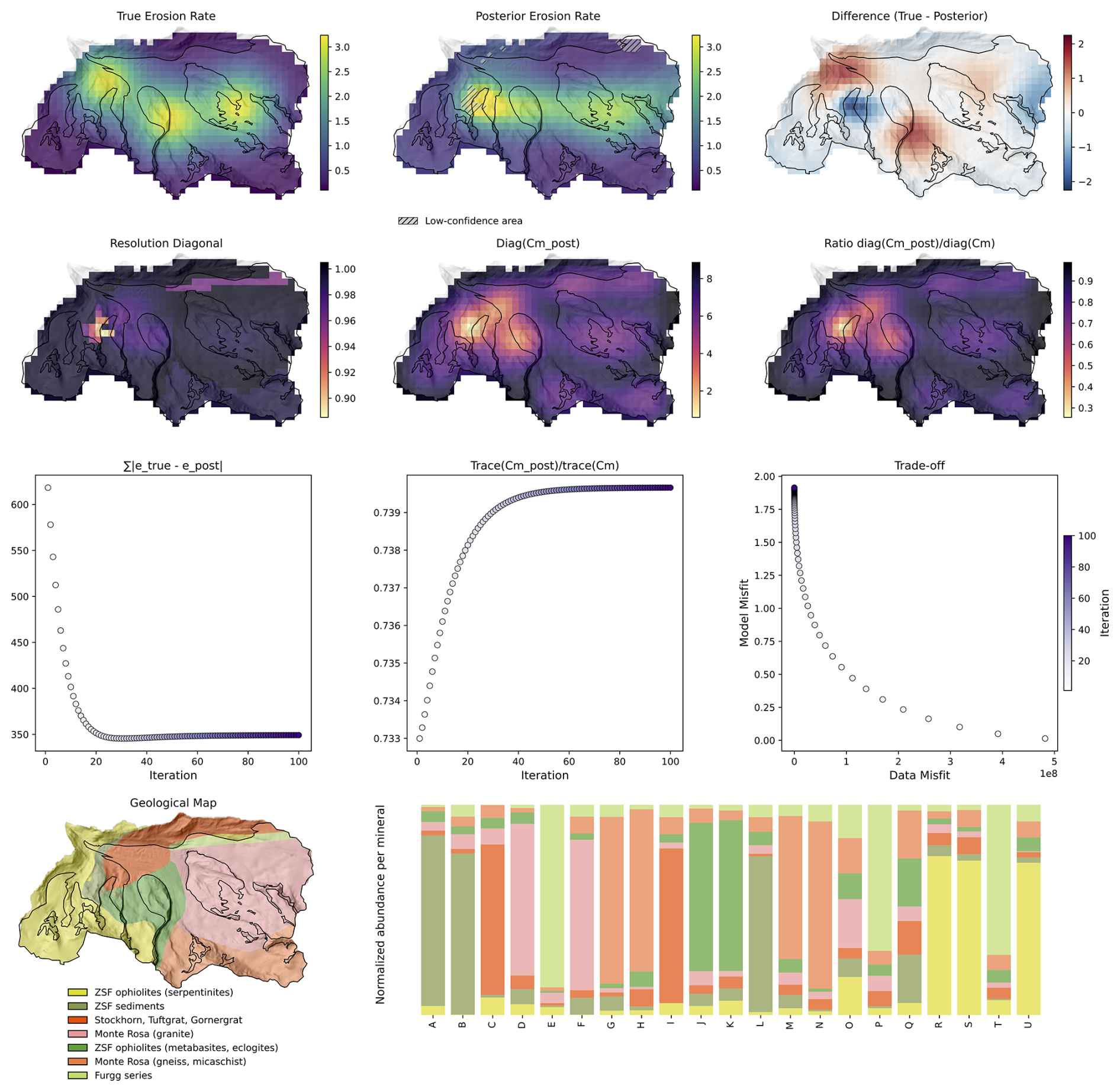
Figure A1 Results of the “three-peak test”: “true” erosion map, posterior erosion map, difference between “true” and posterior erosion map, resolution diagonal, posterior covariance diagonal, normalised posterior covariance, sum of difference between “true” and posterior erosion map during non-linear iterations, normalised posterior covariance during non-linear iterations, trade-off between data- and model misfit during non-linear iterations, geological map, synthetic source tracer concentrations.

Appendix B: Erosion rate map results for scenario tests

In the following figures, we present the detailed results for the three examples shown for each full scenario test. For each figure, the true erosion rate map is displayed on the left, followed by the corresponding results for the three example cases.

Figure B1 illustrates the results for the different geological map configurations: the original geological map, a slightly modified map, and the geological map adapted from Steck et al. (2015). These examples demonstrate how variations in the geological framework affect the recovered posterior erosion rate patterns.

Figure B2 shows the effect of progressively increasing blending of tracer signals. As the tracer fingerprints become more similar, the posterior erosion rate maps become increasingly diffuse. In the most extreme case, where tracer signals are almost fully blended, the inversion does not converge to a solution and the resulting erosion rate map is empty.

Figure B3 illustrates the influence of the number of tracers used in the inversion. As the number of tracers increases, the posterior erosion rate map more closely resembles the true erosion rate map.

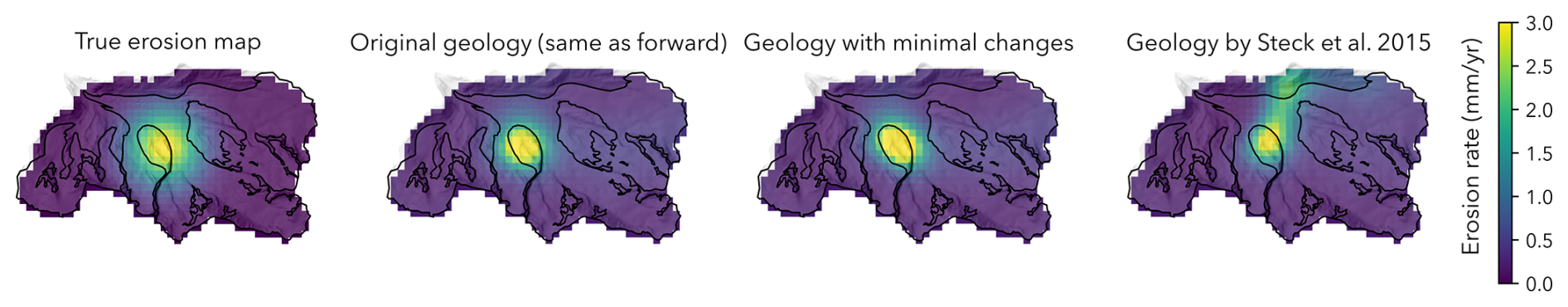
Figure B1 Scenario 1: geological map uncertainty and its impact on posterior erosion rate maps.

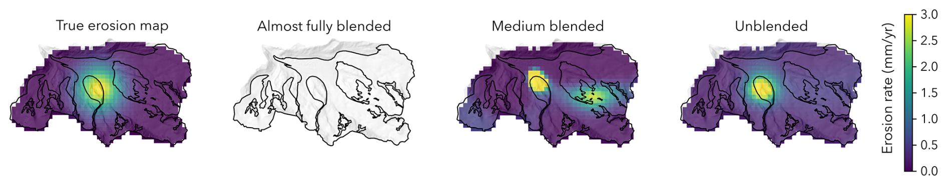
Figure B2 Scenario 2: blended fingerprints: impact on posterior erosion rate maps.

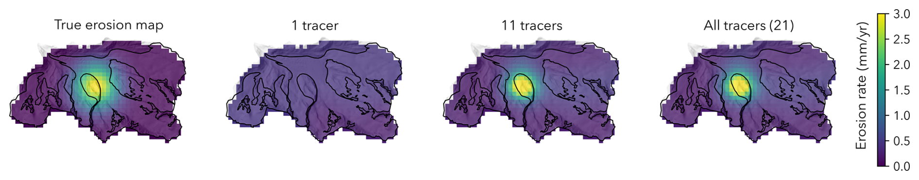
Figure B3 Scenario 3: reduced number of tracer minerals: impact on posterior erosion rate maps.