ImageGrains 2.0: Improved precision and generalization for grain segmentation

Recent advances in deep-learning-based image segmentation have enabled the development of automated approaches to detect individual grains and measure them for geoscientific applications. These methods facilitate the creation of much larger and more precise datasets than traditional manual grain measurements. However, they typically perform best as specialized models trained on homogeneous, task-specific datasets, and often show reduced accuracy when used on different data types.

Here, we present an updated framework, ImageGrains 2.0 that leverages Cellpose-SAM, a recently published next-generation deep-learning model originally developed for cell segmentation in biomedical research. It currently represents the state-of-the-art for dense segmentation in 2D and 3D biomedical datasets. It yields robust results and is capable to generalize across distinctly different image datasets. These properties allow us to re-train the model with geoscientific datasets comprising annotated images of fluvial gravel, coarse pro-glacial deposits, and X-ray computer tomography scans of glacial till and marine sand. We benchmark the segmentation performance of our method against ground-truth annotations, compare it to the performance of other segmentation methods, and we evaluate its measurement accuracy. Our results indicate that this approach outperforms existing methods and confirm that the outstanding performance of Cellpose-SAM is transferable to segment sediment grains. We analyze the size and shape of these segmented grains and find that an increase in grain segmentation accuracy leads to more precise and realistic morphometric results, e.g., more accurate grain size distributions. Additionally, we introduce an interactive graphical user interface for image annotation and correction of model predictions, facilitating the use of the framework for a broad range of image settings. Furthermore, this study underscores the importance of curating more publicly available datasets, which could pave the way towards the generation of a foundation model for segmenting granular particles in geoscientific imagery.

1 Introduction

Data on the size and shape of granular particles have been used across a broad range of geoscientific research areas, and such information has provided the basis for the quantification of the physical and chemical properties of clastic materials (e.g., Sklar, 2024; Israeli and Emmanuel, 2018). Grain morphometry, for instance, is essential for studying sediment production and transport dynamics in environments such as fluvial, marine, glacial, and hillslope systems (e.g., von Eynatten et al., 2012; DiBiase et al., 2017; Allen et al., 2017; Garefalakis et al. 2024). Such data on grain morphometry, particularly those collected in fluvial systems, have proven essential for understanding river hydraulics (e.g., Rickenmann and Recking, 2011; Dunne and Jerolmack, 2018), the mechanisms of sediment transport (e.g., Piégay et al., 2020; Tofelde et al., 2021), and the interplay between fluvial hydraulics and bedload transport (e.g., Dietrich et al., 1989; Pfeiffer et al., 2017; Schlunegger et al., 2020; Deal et al., 2023). Moreover, the sediment particles' size and shape bear information on their transport through various geomorphic processes (e.g., Attal and Lavé, 2009; Miller et al., 2014; Novák-Szabó et al., 2018; Marc et al., 2021), and even on transport conditions on other planets (e.g, Szabo et al., 2015). Furthermore, distributions of the grains' size and shape as well as the geometric arrangement of the clasts in the stratigraphic record (e.g., imbrication) allow to reconstruct deposition events and conditions (e.g., Spagnolo et al., 2016; Schlunegger and Garefalakis, 2018; Biguenet et al., 2021; Preusser et al., 2021).

Despite the importance of quantitative and robust data on grain size, shape and orientation, obtaining such data remains a challenge. Traditionally, data on the grains' morphometries have been collected through manual measurements of grains in the field or through sieving (e.g., Bunte and Abt, 2001; Watkins et al., 2020; Baynes et al., 2020; Garefalakis et al., 2023), from topographic point clouds (e.g., Vázquez-Tarrío et al., 2017; Woodget and Austrums, 2017; Steer et al., 2022) or from imagery (e.g., Ibbeken et al., 1986; Butler et al., 2001; Carbonneau et al., 2004; Detert and Weitbrecht, 2012; Buscombe, 2013; Sulaiman et al., 2014; Purinton and Bookhagen, 2019). Manual measurements are laborious, typically yield low numbers of observations (e.g., Eaton et al., 2019) and are prone to bias (e.g., Daniels and McCusker, 2010), especially when traditional geometric sampling techniques, e.g., Wolman counts or line sampling (Wolman, 1954; Fehr, 1987) are used. Obtaining grain geometries from topographic point clouds is often limited by the technical limits of the acquisition method, grain occlusion or necessary geometric assumptions for grain segmentation (e.g., Steer et al., 2022; Woodget and Austrums, 2017). Image-based methods require field calibration for texture-based approaches and often manual correction of individual grains for segmentation-based methods; both digital methods also tend to systematically over- or underestimate grain sizes (e.g., Chardon et al., 2022; Mair et al., 2022).

In the past years, machine-learning tools have been developed in an effort to automate the measurements of grain size and shape in images to improve data quality, and to allow for an increase in number of observation. Among these, texture-based methods predict percentile values of grain size distributions if an unambiguous correlation between an image texture and a characteristic grain sized distribution exists, and if these were included in the training data (e.g., Buscombe, 2020; Lang et al., 2021). In contrast, segmentation-based methods delineate individual grains through object detection (Chen et al., 2022; Mair et al., 2024; Miazza et al., 2024; Sylvester et al., 2025) and facilitate the creation of large datasets, which allow for size and shape analysis down to the individual grain level. However, these segmentation models work best when trained as narrow specialist models on homogenous datasets, which often require task-specific, and sometimes site-specific, training and careful curation of the corresponding datasets (e.g., Chen et al., 2023; Prieur et al., 2023; Azzam et al., 2024; Miazza et al., 2024; Zegers et al., 2025; Schuster et al., 2026).

During recent years, a new generation of deep learning models that use a transformer architecture has become widely used in the field of computer vision for tasks related to the segmentation of objects in images (e.g., Dosovitskiy et al., 2021; Li et al., 2022). This resulted in the development of foundation models, such as the Segment Anything Model (SAM; Kirillov et al., 2023; Ravi et al., 2024), which are trained on very large and general datasets. These foundation models have proven effective at generalization, i.e., being able to predict outcomes for previously unseen data, which were not used for training. Due to a strong inductive bias, they are also considered as effective at out-of-distribution detection of objects, especially when fine-tuned on smaller datasets (Hendrycks et al., 2020; Fort et al., 2021). While these models perform well at segmenting numerous different types of objects in images, they are less efficient at accurately segmenting large quantities of a narrow range of objects, especially when they are not fine-tuned to specific datasets or when no specific prompts are used (Sylvester et al., 2025; Chan et al., 2026).

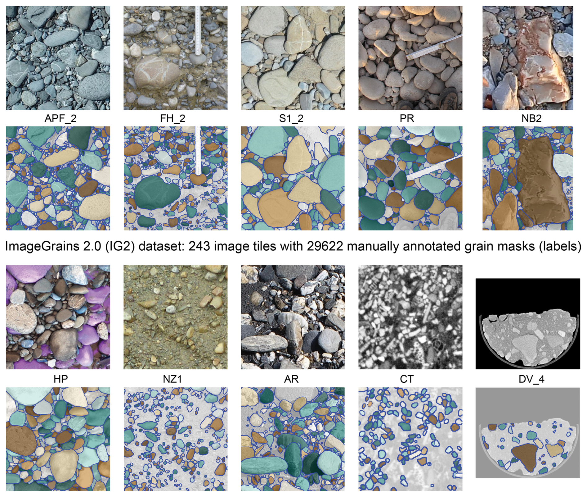
Figure 1 Example images and their manually annotated grain masks (labels) for various types of imagery and grains used in the IG2 dataset, and their respective indicated subset (Mair et al., 2025a; see Table 1 for more details). For visual examples of images with non-grain objects (e.g., vegetation) refer to Fig. S1. Individual grains are shown in random colors with blue outlines. Please note that the examples for FH_2 and NZ1 are images taken from near vertical outcrops, where finer-grained background sediment cannot be resolved and therefore is not annotated.

Here, we present an update to the ImageGrains framework by Mair et al. (2024) that introduces two major improvements. First, it leverages the strengths of Cellpose-SAM (Pachitariu et al., 2025), a recently published next-generation deep-learning model originally developed for cell segmentation in biomedical imagery. This model eliminates weaknesses of SAM and improves the performance for dense segmentation of many instances of the same object type with high accuracy, while maintaining the outstanding generalization ability. We utilize the new Cellpose-SAM model that was trained on large datasets of predominantly biomedical imagery of cells (for details, see Pachitariu et al., 2025) and retrained it to find grains in images of clastic sediment. This transfer learning approach allows us to utilize both the representations learned by SAM that enable the generalization across widely differing datasets and data types, and the Cellpose segmentation framework (Stringer et al., 2021) that facilitates the efficient and dense segmentation of grains with high accuracy without the necessity of prompt engineering. To achieve this, we newly curated a dataset of 162 annotated image tiles, which we combine with the existing ImageGrains 1.0 dataset to obtain a set of 243 image tiles from various types of sediment grains (Fig. 1). This increase in number of annotated images constitutes the second major improvement compared to the previous version. We then compare the segmentation results of our re-trained Cellpose-SAM model with the results of other state-of-the-art approaches, and we test the models' ability to generalize by using subsets of our dataset as unseen test splits. Finally, we highlight the potential of applying our workflow to 3D datasets of stacked images retrieved by X-ray computer tomography (CT) scans. Our results indicate that the new framework outperforms existing methods both in accuracy of the resulting segmentation, and in the capability to segment grains in new types of imagery.

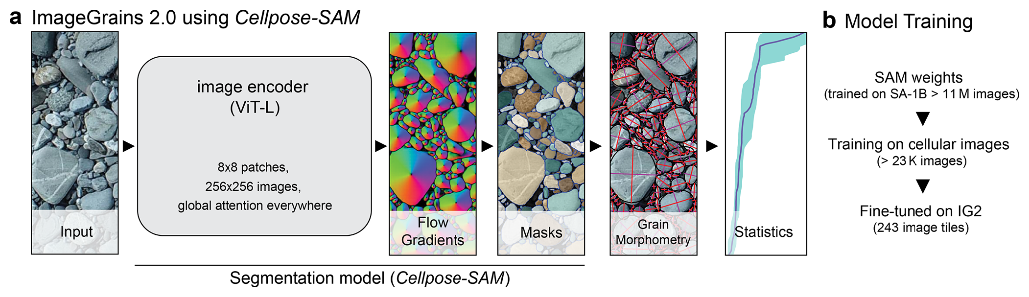
Figure 2 Overview of our workflow (a) that uses a re-trained Cellpose-SAM (Pachitariu et al., 2025) architecture for grain segmentation. The re-training (b) was done by fine-tuning Cellpose-SAM to the IG2 dataset (see Table 1 for more details). ViT-L refers to the model weights used to initialize SAM, and SA-1B indicates the original training dataset of SAM (Kirillov et al., 2023). For details on the architecture of the segmentation model, refer to Pachitariu et al. (2025) and references therein.

2 Methods

For ImageGrains 2.0, we employ the recently released Cellpose-SAM (Pachitariu et al., 2025) model architecture for segmenting biomedical images, which itself utilizes the Vision Transformer (ViT) of the Segment Anything Model (SAM; Kirillov et al., 2023) as backbone together with the gradient tracking of the original Cellpose framework (Stringer et al., 2021). Similar to the approach of Mair et al. (2024), we use a dataset consisting of images with annotated sediment grains (Fig. 1). In contrast to the dataset used by Mair et al. (2024), ImageGrains 2.0 (IG2; Mair et al., 2025a) is based on a much larger dataset including more image types (see Sect. 2.1). We use the IG2 dataset to train our model. We also evaluate its capability to quantify the size and shape of sediment grains (Sect. 2.2). In our approach, we apply transfer learning and retrain the pre-trained Cellpose-SAM foundation model to segment grains in images taken from clastic sediments (Fig. 2). In Sect. 2.3, we summarize key aspects of this foundation model and the adaptations we made. Next, we describe how we set up other methods and models that we use to benchmark our approach (Sect. 2.4). We then proceed by quantifying and comparing the segmentation performances across all methods (Sect. 2.5). Finally, we obtain a set of aggregated metrics, which are based on the measured sizes and shapes of individual grains, to evaluate the effect of using segmented grain masks with varying precision. We note here that we use the term method for entire segmentation workflows, while the term model refers to a specific segmentation model. This distinction becomes important as some methods combine several models and we sometimes train several models using the same method with different datasets.

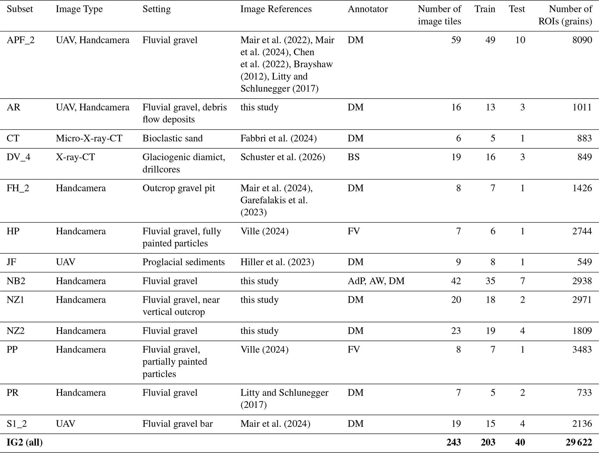
Table 1 Dataset composition, image type, setting and summary statistics for the ImageGrains 2 (IG2; Mair et al., 2025a) dataset. ROI = region of interest.

2.1 The ImageGrains 2.0 (IG2) dataset

The IG2 dataset (Mair et al., 2025a) comprises over 29 000 manually annotated 2D masks of individual sediment grains captured in diverse image types, including RGB imagery taken from uncrewed aerial vehicles (UAVs), single-lens reflex cameras, compact digital cameras, and X-ray computed tomography (CT) slices (Table 1). Annotated grains cover a broad range of sedimentary contexts, including fluvial gravels in outcrops (Garefalakis et al., 2023), fluvially transported pebbles, cobbles, and boulders on gravel bars and in river channels (Litty and Schlunegger, 2017; Mair et al., 2022; 2024), bioclastic sands from marine lagoons (Fabbri et al., 2024), and glaciofluvial deposits (Hiller et al., 2023; Schuster et al., 2026).

To create the IG2 dataset, we both expanded the existing subsets of the ImageGrains 1.0 dataset (IG1; Mair, 2023) and added new subsets. First, we added 5 additionally labelled image tiles to IG1 to improve the balance between the different image settings and data sources (Table 1) in the respective test and training splits. In particular, we added 1 image of a vertical gravel outcrop in the FH_2 subset, 1 image tile from the Swiss Sense River in the S1_2 subset, and 3 image tiles of fluvial pebbles from variable sources in the APF_2 subset. Second, we created 6 new subsets containing a total of 103 image tiles taken from fluvial sediments of rivers in Spain (with grains fully and partially painted in the field to track grain mobility and mobilization; HP, PP; Ville et al., 2023), Peru (PR), New Zealand (NZ2), Switzerland (AR), and Namibia (NB2). Furthermore, we included two more subsets of image tiles taken from coarse-grained and angular proglacial sediment (JF), and images retrieved from near-vertical outcrops of lithified conglomerates (NZ1). The images were acquired with different handheld and uncrewed aerial vehicle (UAV)-borne camera systems (Table 1) at varying resolutions. Finally, we completed the dataset by using X-ray CT (XRCT) scans taken from glacial tills (DV4), and micro-CT images of bioclastic marine sand (CT), which we annotated in two respective subsets. All these images were selected for variations regarding the objects displayed on the images. This includes – on purpose – the occurrence of vegetation and other objects that are not sediment grains to test the model against the possibility of false detections. We did so in order to challenge the models beyond variabilities in lithology, color, grain size and shape of the clasts. Specifically, we selected tiles that depict various objects such as scales, hands and equipment; tiles that featured different types of vegetation and water bodies (see Fig. S1 in the Supplement for examples of non-grain features), and that were acquired under variable light conditions. The combination of all subsets resulted in a total of 203 and 40 annotated image tiles that we used for training and testing, respectively.

To train and test segmentation models that are able to map a large variety of sediment grains on different image types, we created labels for the newly used image data. For each image that was used in the expanded IG2 dataset, we chose subset tiles of varying sizes (ranging from 50 pixel × 62 pixel to 2750 pixel × 2000 pixel) that capture the full grain size variability and the complexity of the image content. This resulted in a large variety of tiles for each image (Table 1). These tiles were annotated manually using the LABKIT plugin (Arzt et al., 2022) for FIJI (Schindelin et al., 2012) and napari (v0.6; napari contributors, 2019), where each grain was labelled individually (i.e., dense labelling) as precisely as possible at the scale of individual pixels. In total, we added 162 such annotated image tiles from various sources and settings to the 81 tiles of fluvial sediment images compiled and annotated for the previous version (IG1). For all datasets, we manually generated representative subgroups of images, called stratified train and test splits (Table 1), to create internally balanced subsets for all imagery from different settings.

2.2 2D Grain morphometry

Aside from quantifying the segmentation performance, we assessed the importance of precisely segmenting grain masks for yielding accurate results using grain size and shape metrics as benchmark information. For each grain mask, or region of interest (ROI), we used standard image analysis tools implemented in scikit-image (v0.25.2; van der Walt et al., 2014) to represent the morphometry of both grain size and shape as well as orientation.

To quantify grain sizes, we fitted ellipses to approximate the shape of the target grains for which we calculated the lengths of the minor and major axes (b- and a-axis, respectively) of an ellipse. This approach has been demonstrated to capture well grain sizes of clastic material in 2D images (e.g., Purinton and Bookhagen, 2019; Chardon et al., 2022; Garefalakis et al., 2023; Mair et al., 2024; Sklar, 2024). The uncertainties of the grain size percentile values are quantified through bootstrapping, thereby resampling any grain size distribution (GSD) 1000 times (for details, see Sect. 2.4 in Mair et al., 2022). We then calculated the differences between grains in the ground truth and predicted grains as difference for the percentile values. Furthermore, we tested if the GSDs of the ground truth and the predictions were statistically different with a two-sample Kolmogorov–Smirnov test. Here, the two distributions being identical was the null hypothesis, which we rejected for p< 0.05. We note that due to the 2D nature of images, an inherent limit exists for detecting grains of small sizes, which itself is controlled by the image resolution (see Sect. 2.5 for details on our approach in this study). An important implication thereof is that the resulting GSDs are truncated at a specific threshold characterizing the smallest measurable size.

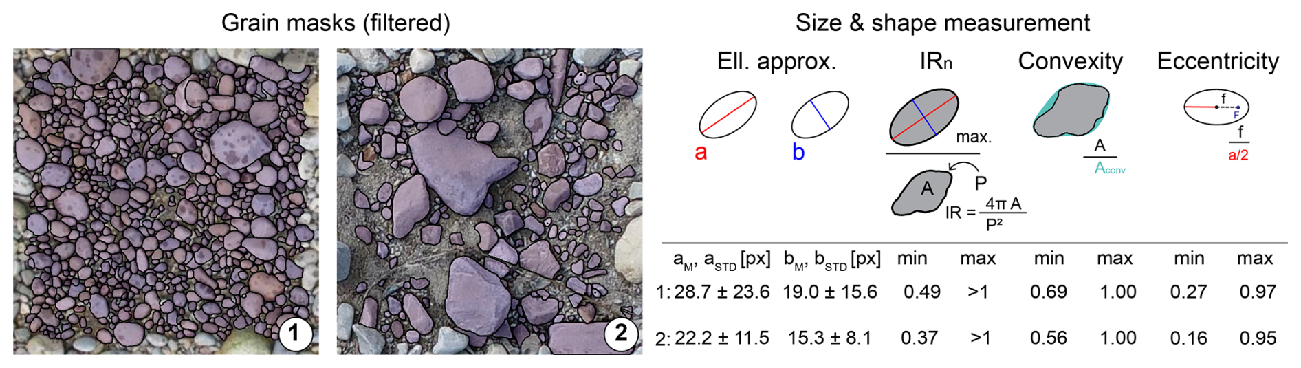
Figure 3 Two examples of how grain size (with mean and 1σ standard deviation values), and shape were measured based on grain mask area and outlines, displayed here for annotated images tiles (labels) from subset APF_2. Ell. approx. = Ellipse approximation, a = major axis, b = minor axis, f = focal length, F = focal point, A = area, A_conv = area of the convex hull, P = perimeter, IR_n = normalized isoperimetric ratio (IR_n, or circularity; Pokhrel et al., 2024), px = pixel. For details on the metrics, refer to Sect. 2.2.

To quantify grain shape and orientation we used several approaches (Fig. 3) that have been successfully applied in recent studies across various geoscientific research fields (e.g., Miller et al., 2014; Szabó et al., 2015; Lepp et al., 2024; Benet et al., 2024; Back et al., 2025a). We calculated the eccentricity, i.e., the ratio of the focal distance over the length of the major axis of the fitted ellipses, to approximate the grain elongation in 2D, which is a classic metric for quantifying the rock fabric (Tucker, 1988). Similarly, we used the convexity, sometimes also called solidity (e.g., in scikit-image; van der Walt et al., 2014), which is the ratio of pixels in the ROI to pixels within the convex hull, as proxy value for the 2D roughness of each grain. This parametrization of grain roughness has been frequently used (e.g., Cox and Budhu, 2008; Lepp et al., 2024) with relatively small differences compared to other parametrizations (Back et al., 2025b). Next, we obtained the isoperimetric ratio (IR) and normalized isoperimetric ratio (IR_n, Pokhrel et al., 2024; Quick et al., 2020) for each grain mask as indicator for the roundness of a grain. We note the selected approaches to compute IR and IR_n values can return values > 1 in some cases, which could be the consequence of geometrically imperfect reconstructions (see supporting information of Quick et al., 2020). Finally, we measure the 2D grain orientation as azimuth angle of the b-axis of the above-described ellipse fit and the y-axis, i.e., the image height, of each image tile in degrees from 0 to 180°. Note that these metrics are an exemplary selection, and that any 2D shape and size metric can be calculated from the segmented grain ROIs.

We calculated all the aforementioned metrics for all ROIs in both ground truth and predicted masks that fall in the central 81 % area of each image tile by avoiding the outermost 5 % from the edge of each image. We did so to avoid a bias that could be introduced by considering grains – possibly cut ones – at the edge of image tiles. We then calculated differences between ground truth grains and predicted grains for all corresponding metrics. By comparing these morphometric values across datasets, we can quantify how the segmentation quality affects the morphometric results.

2.3 Cellpose-SAM: re-training and inference

The Cellpose framework (Stringer et al., 2021) used a deep-learning model, which is based on a U-Net (Ronneberger et al., 2015) type of neural network with image style transfer (Gatys et al., 2016), a widely employed architecture that has proven very successful in image segmentation tasks (Siddique et al., 2021; Azad et al., 2024). This framework was combined with an equation modelled on heat diffusion to predict vector flows. From these flows, individual objects are segmented through gradient tracking. In Cellpose-SAM the previous backbone model was replaced with a modified version of the SAM transformer (Kirillov et al., 2023; see also Sect. 2.4.1 below for more details on SAM). Specifically, it used the image encoder module of SAM and replaced the decoder parts with Cellpose's flow representation for prediction (Pachitariu et al., 2025). Moreover, the encoder itself was modified in several ways for the Cellpose-SAM architecture. First, the dimension of the input image was reduced to 256 pixel × 256 pixel (from 1024 × 1024), and the patch size was reduced to 8 × 8 (from 16 × 16). This was done in an effort to decrease the processing time and to decrease computational costs. Accordingly, the position and patch embeddings were also downsampled, while global attention was used for all layers. This approach differed from using a global attention in only some layers in the original SAM architecture. It aims to improve the performance of tasks where dense segmentation is required, i.e., where multiple objects of the same class are segmented (for more details, refer to Pachitariu et al., 2025). The Cellpose-SAM model was initialized with the SAM ViT-L (large) model weights, which allow for faster inference while maintaining a high segmentation quality compared to ViT-H (huge; Kirillov et al., 2023). Both ViT-L and ViT-H had been trained on the SA-1B dataset (Kirillov et al., 2023). Pachitariu et al. (2025) then trained Cellpose-SAM on an updated dataset of 22826 cell and cell nuclei images with  > 3.3 million labelled objects. Notably, the updated architecture is much larger (> 304 million trainable parameters compared to > 6.6 million trainable parameters in the old U-net model). Furthermore, the improved model can use multi-channel images, i.e., color images, because of its training with random permutations of channels. This was not possible with the previous models that converted the images to single-channel greyscale images before the segmentation. As a result, multi-channel images are now the default image input.

We retrained the Cellpose-SAM model on our IG2 dataset using default settings and follow recommendations of Pachitariu et al. (2025) for the custom re-training to obtain our new default model for ImageGrains. Our setup differs from that of Pachitariu et al. (2025) in terms of the training length (we trained our model for 500 epochs instead of 100). We did so, in an effort to maximize the learning of the model. For training, we used all 203 image tiles of the train split in every epoch, and it was accomplished within < 1.5 h on a NVIDIA A100 GPU with 80 GB memory at the UBELIX HPC cluster maintained by the University of Bern. The image tiles from the test split were used for validation every 10 epochs. By default, the learning rate increased linearly from zero to 1 × 10⁻⁵ over the first 10 epochs, and then decreased by a factor of 10 every ten epochs over the last 50 epochs. The loss function was the default Cellpose segmentation loss, which is the mean squared error between the 2D flows (in the XY plane; Pachitariu et al., 2025). This error is calculated for the ground truth and the predicted flows, to which the cross-entropy between the probabilities of the ground-truth and the predicted objects is added. During the training, the images were randomly flipped, rotated and resized using a uniformly distributed scaling factor between 0.5 and 1.5 before they were randomly cropped to 224 pixel × 224 pixel. By default, all image tiles were normalized to image intensity percentiles between 1 and 99 for each channel, and the AdamW optimizer (Loshchilov and Hutter, 2019) together with a weight decay factor of 0.1 was used.

Upon evaluating the model on 2D images, we again employed the default settings of Cellpose-SAM, which include a block tile size of 256 pixels, a fractional tile overlap of 0.1, a threshold value of 0.0 for the object probability, and 0.4 for the flow error, respectively. Again, the image intensity was normalized to the percentile range of 1 to 99 for each input channel. All of these settings were kept at default values of the algorithm, due to their demonstrated effectiveness (Pachitariu et al., 2025). Contrary to previous Cellpose versions, no rescaling of image tiles was applied. For 3D segmentation, we used the dedicated 3D approach of Cellpose (Stringer et al., 2021), which computes 2D flows and probabilities for slices in the XY, YZ, and XZ planes (Stringer and Pachitariu, 2025). The resulting values are then averaged to create 3D flow vectors. For the construction of 3D segmentation masks, which themselves are generated from the 3D flow vectors, we used the default computation, which considers a 3D smoothing factor of 1.0. This default setup allows for a high-quality 3D segmentation despite upscaling from 2D segmentations (e.g., Zhou et al., 2025). For the demonstration of our 3D segmentation performance, we used a stack of 400 TIFF images generated with XR-CT of a drill core (from site 5068_1_C from 4–5 m depth) taken from a glacio-fluvial sediment infill in a glacially over-deepened valley in southern Germany (Schuster et al., 2024). For details on the XR-CT scanning and image reconstruction, we refer to Schuster et al. (2026).

2.4 Other methods and models

We explored how well our approach compares to other methods that were publicly available at the time of writing this article and that were either used as a foundation model for general object detection or that were specifically tailored to segment grains. Note that we did not include the methods of Mörtl et al. (2022), Chen et al. (2024), or Soloy et al. (2020), because their models or code were not publicly available. Furthermore, we did not include the method of Chen et al. (2022) because of its relatively weak performance in previous studies (Mair et al., 2024).

We first compared the outcome of our segmentation with that of SAM (Vit-H) in its basic configuration to generate masks. We viewed the performance of SAM as a baseline benchmark that every dedicated method should exceed, due to its capability to segment grains on a broad range of image datasets and object types (Kirillov et al. 2023) without fine-tuning for specific data, such as sediment grains. Next, we compared our results to the results of Segmenteverygrain that uses prompt engineering for improving segmentations by SAM (Sylvester et al., 2025). Here, we used both their default prompt engineering model, SEG-SAM (default), and one that we trained on our IG2 dataset, SEG-SAM (IG2). Finally, to evaluate the relative improvement in segmentation performance with our new default model, we compared its segmentation results with those of the best performing model of Mair et al. (2024). In a second step, we evaluated our default model's ability to generalize to data not used during training with a setup where the S1_2 and PR subsets were excluded from training. We selected these two subsets for this test because for these subsets, the performance of both our fine-tuned Cellpose-SAM model and most benchmark models was highest amongst all subsets with heterogeneous image tiles of fluvial pebbles. Hence, we anticipated the largest impact on the segmentation performance if we left out these data from the training split. Particularly, we compared the performance of our default model to that of all other models including specialized Cellpose v2 models, which were trained only on subset datasets used in this generalization.

In the following section, we briefly describe how we set up all benchmark models.

2.4.1 The Segment Anything Model (SAM)

SAM is a foundation segmentation model with a vision model transformer (Dosovitskiy et al., 2021; Li et al., 2022) that has been highly successful in segmentation tasks (Na et al., 2024; Archit et al., 2025). SAM itself was pre-trained with images from a large dataset of annotated images (11 million images with over 1 billion annotation masks; SA-1B) that was created with a custom data engine (Kirillov et al., 2023). This model can thus be used for segmenting a broad range of objects, and it is adaptable to more specific requirements related to various downstream tasks via prompt engineering, which is inspired by similar advances in Natural Language Processing (Brown et al., 2020). The model itself consists of an image encoder, a mask decoder for inference, and a prompt encoder that is employed for flexible prompt handling (Kirillov et al., 2023). We used the largest available model checkpoint ViT-H (huge), which demonstrated the highest segmentation precision (Kirillov et al., 2023), together with its default mask decoder, to predict grain masks. For this zero-shot instance segmentation (i.e., segmenting objects in images that had not been included upon training the model), the model generates a grid of point prompts, for which it then filters low quality and duplicate masks. We used the predictions resulting from this model setup as baseline benchmark for grain segmentation without custom method developments because they are based on data that is openly accessible. In addition, these predictions can be achieved without any fine-tuning or supervised training on images that display sediment grains.

2.4.2 Segmenteverygrain

Segmenteverygrain combines SAM (i.e., the ViT-H checkpoint; see Sect. 2.4.1 for details) with a U-Net style convolutional neural network for the prompt engineering upon segmenting grains in images (Sylvester et al., 2025). The default U-Net model was trained on 66 different images displaying grains. The images themselves were split into 44 533 patches of 256 pixel × 256 pixel. We used both the default model and a model, which we fine-tuned with the entire IG2 dataset. Here, we employed the default train/test splits of our IG2 dataset and the test split for validation to ensure comparability with the other fine-tuned models. Aside from this, we used the default configuration of Segmenteverygrain and followed the recommendation for fine-tuning it (Sylvester et al., 2025). This configuration included the Adam optimizer and image augmentation. We trained the refined model for 500 epochs and set the minimum object size to 15 pixels in order to match similar values of other models. We used the predictions of Segmenteverygrain as benchmark for the approach referred to as prompt-based segmentation.

2.4.3 Cellpose  2 models

To evaluate the impact of both the expanded dataset (IG2) and the new backbone architecture, we compared the segmentation results of Cellpose SAM with those of older Cellpose (v2.3) models. We started by using the IG1_full_set model of Mair et al. (2024), Cellpose  2 (IG1), which was trained on their original dataset that roughly comprised a third of the images of the IG2 dataset (i.e., subsets S1_2, APF and FH; see also Sect. 2.1 for details on the datasets). We then trained a Cellpose  2 model (Pachitariu and Stringer, 2022) with the same architecture on the full IG2 dataset, Cellpose  2 (IG2), using the same hyper-parameters and configuration as in the original publication (Mair et al., 2024). This included training any Cellpose  2 model for 1000 epochs, a learning rate of 0.2 with a step-wise reduction of the learning rate by a factor of 2 for every 10 epochs during the last 100 epochs and a batch size of 8 single-channel images, thereby employing the default Cellpose implementation for image augmentation. Furthermore, Cellpose models can be trained as specialist models if fine-tuned to a specific dataset (Stringer et al., 2021; Mair et al., 2024). Therefore, we trained two more Cellpose  2 models on the IG2 dataset but without the S1_2 and PR image tiles. For further fine-tuning, we re-trained them only on the respective subsets S1_2 and PR.

2.5 Evaluating segmentation performance

We quantified the segmentation performance by first evaluating how closely individual prediction masks are representing ground truth annotations on an object (ROI) basis followed by calculating a precision score based on the number of grain masks that exceed an accuracy threshold (Everingham et al., 2015). This was done by comparing the predicted grain masks to the best-matching masks in the ground truth labels using the approach of Stringer et al. (2021) calculating average precision (AP) scores, evaluated at different intersection-over-union (IoU) thresholds. Specifically, we calculated the IoU metric for each grain mask with its closest ground truth match. We used an IoU threshold of > 0.5 (for AP@0.5), and the increasingly stricter range of 0.5 to 0.9 (to calculate the average of AP values, i.e., mAP) to determine which grains were considered as true positives (TP). Grain masks in the ground truth that were not matched by a predicted mask with an IoU value above the aforementioned thresholds were counted as false negative (FN). Likewise, predicted grains with no corresponding grain mask in the ground truth that met the IoU quality criteria were considered as false positive (FP). The average precision was then calculated as the ratio between TP, and the sum of TP, FN and FP, i.e., $\text{TP}/(\text{TP}+\text{FN}+\text{FP})$.

We used these standard metrics in object detection (e.g., Padilla et al., 2020; Yang et al., 2023; Zhou et al., 2025) to quantify the quality of the segmented grains, based on individual ROI quality, and to compare the results with those of the other methods. We chose to use this object-based metrics because they combine both false negative and false positive detections in a single step, making it a more stringent metric than traditional metrics, such as precision, recall, or simple intersection over union (IoU) scores (e.g., Minaee et al., 2022). Furthermore, the average precision and mean average precision scores are ubiquitous metrics used to evaluate object-detection models in the field of computer vision, which includes models such as SAM (Kirillov et al., 2023), YOLO (Redmon et al., 2016) or Mask R-CNN (He et al., 2018), among others.

Similar to the approach of Mair et al. (2024), we excluded grains for which the minor axis of a simple ellipsoidal fit was < 8 pixels both in the ground truth and in the segmented grain masks. The reason for this is that for most image types displaying sediments, we find it difficult to consistently distinguish between grains that are smaller than 8 pixels during image annotation, which might render any predictions of smaller grains unstable. We acknowledge that this threshold value can vary across different image settings, e.g., it is usually easier to identify very small grains in single-channel CT images with a high contrast than in multi-channel color images taken from fluvial sediments with a coarser resolution. This is in line with similar but larger thresholds (i.e., 20 or more pixels) determined by other approaches on similar fluvial sediment imagery (e.g., Chen et al., 2022; Purinton and Bookhagen, 2019; Chan et al., 2026).

3 Results

3.1 Grain size and shape in ground truth ROIs

We first calculated standard 2D grain morphometry metrics (Fig. 3) for more than 18 500 manually labelled masks (ROIs) that remained after filtering for minimum grain size and distance to image tile edges. These manually labelled masks represent about 63 % of all labelled ROIs (for train and test split combined; Table 1). The resulting grain sizes vary substantially across the dataset, with b-axis lengths ranging from 8.0 to 481.0 pixels and a-axis lengths from 9.1 to 713.2 pixels (Table S1 in the Supplement). The mean grain sizes reflect this variation of more than one order of magnitude, with average b-axis lengths ranging from 10.8 ± 2.7 pixels (CT) to 100.3 ± 111.3 pixels (NZ2). Within each data subset, grain sizes are highly variable, and systematic differences in mean grain size are observed between subsets for both a- and b-axes (Table S1).

The measured grain shapes vary among the data subsets. For grain roughness, expressed by the convexity values, the average of the unitless ratio for the overall dataset is 0.93 ± 0.05, which is consistent with the averages of the respective data subsets, despite their high within-subset variability (Table S1). For example, the convexity shows a strong variability in some individual image tiles, with values ranging between 0.62 and 1.00. In general, a greater variation is observed for grain roundness values, expressed by the normalized isoperimetric ratio (IR_n, or circularity). Whereas the respective values generally range from 0.38 to > 1.0, the average IR_n values across data subsets range from 0.83 ± 0.07 (DV_4) to 0.97 ± 0.04 (CT), indicating systematic differences in roundness values between subsets (Table S1). The average value of IR_n of 0.89 ± 0.09 calculated on the basis of the image tiles also reflects this broad variability. The data representing the grain elongation shows the largest variability where the eccentricity values for grain ellipse-approximations range from 0.25 to 0.97. Despite this broad range, the average eccentricity values of the data subsets are consistent with each other and yielding an average of 0.73 ± 0.14, again demonstrating a strong within-subset variation (Table S1).

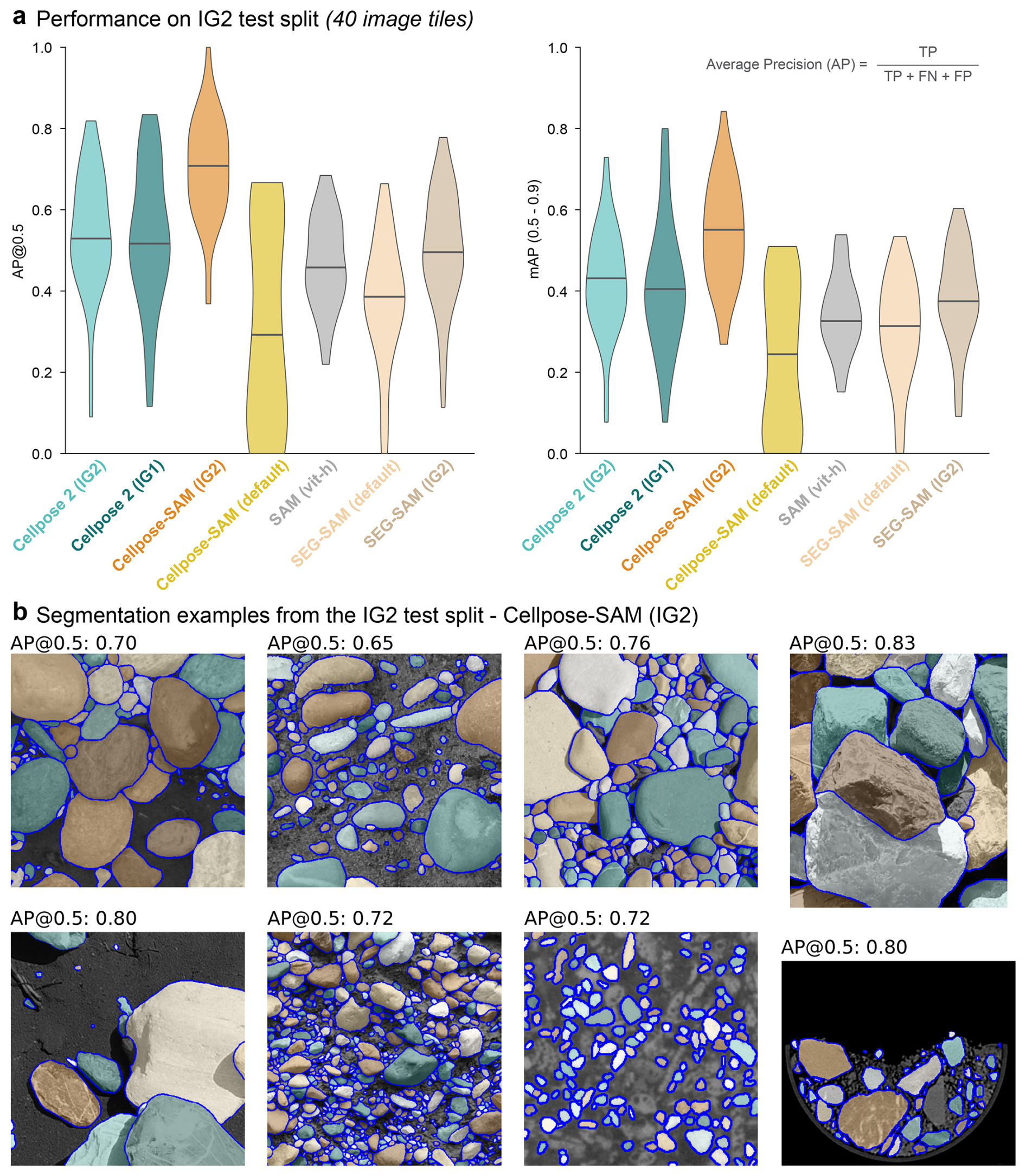
Figure 4 Segmentation results for the IG2 test split calculated on an image-tile-basis with performance of the tested methods or models (a), and examples of predicted grain masks (b). AP@0.5 = average precision evaluated at the intersection-over-union (IoU) threshold of 0.5; mAP = mean average precision for IoU thresholds ranging from 0.5 to 0.9; TP = true positive, FP = false positive, FN = false negative. SEG-SAM = Segmenteverygrain.

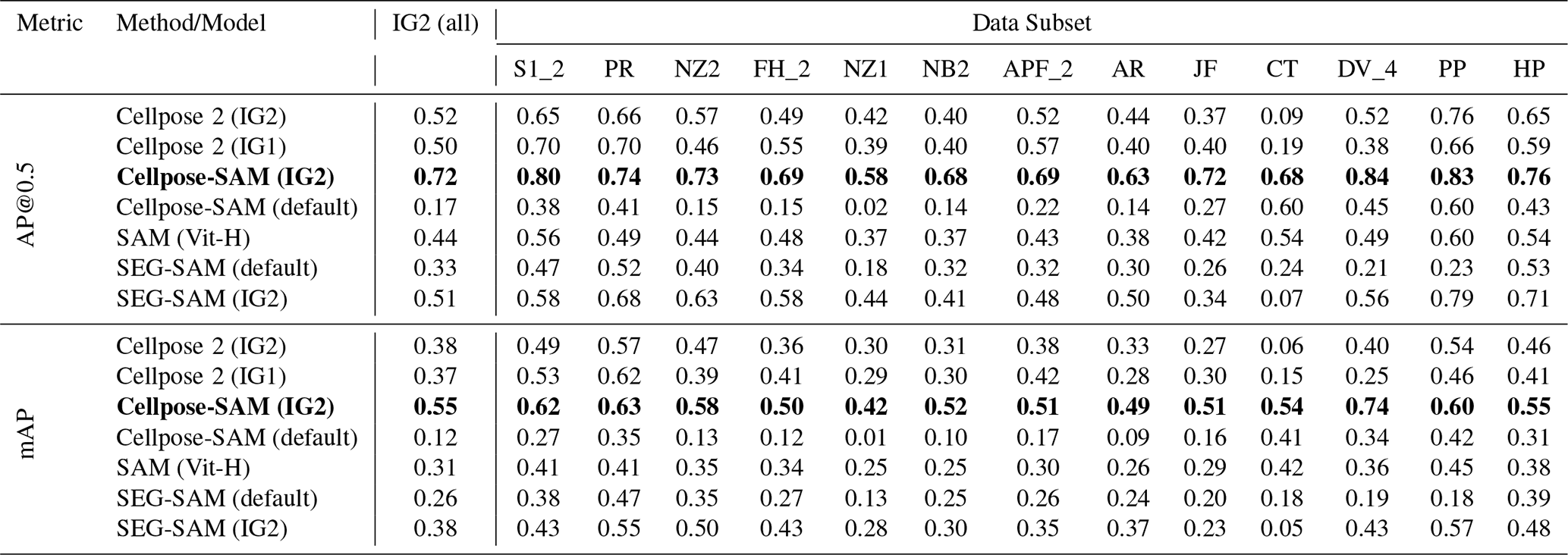
Table 2 Segmentation performance of all methods and models for the annotated grains in the IG2 dataset (test and train splits combined), and its subsets with the best performing model indicated in bold. All values are mean AP@0.5 or mAP values for all image tiles in the respective subsets, while for the entire dataset (IG2 –all), we report the median performance across all image tiles. Please note that the values for IG2 (all) are calculated on an image basis and therefore they are not the average of the respective values reported for the data subsets in the right part of the table. AP@0.5 = average precision evaluated at the intersection-over-union (IoU) threshold of 0.5; mAP = mean average precision for IoU thresholds ranging from 0.5 to 0.9.

3.2 Segmentation performance

Overall, our default segmentation model, Cellpose-SAM (IG2), achieves a high accuracy in grain segmentation across all image types and most subsets (AP@0.5 > 0.6; mAP > 0.5 for train and test splits combined; Table 2; Fig. 4). Notably, the performance was largely independent from the dataset balance, i.e., the number of image tiles in a subset and its relative share of the entire dataset. For example, the segmentation performance for image tiles from subset DV_4 scores highest among all subsets (with an AP@0.5 value of 0.84; Table 2), despite their image type of XR-CT images accounting for only around 10 % of all the image tiles in the dataset (Table 1).

Compared with alternative approaches, Cellpose-SAM (IG2) consistently outperforms all other models if evaluated on both the full IG2 dataset and across subsets (Table 2). This advantage is maintained in both training and test splits (Table S2 in the Supplement; Fig. S2 in the Supplement). Specifically, the median AP@0.5 across all test image tiles is 18 % higher than that of the second-best method (0.71 vs. 0.53 for Cellpose  2 trained on IG2; Fig. 4a; Table S2), and 20 % higher across all image tiles (0.72 vs. 0.52 for Cellpose  2 trained on IG2; Table 2). The performance of the fine-tuned Cellpose-SAM (IG2) model remains robust even for challenging image tiles, with almost no prediction-scoring AP@0.5 values below 0.4 (Figs. 4a and S1).

Upon comparing the performance of the methods other than our fine-tuned Cellpose-SAM (IG2), three observations can be made. First, the second-best models (using both the test and the full datasets) were trained with the IG2 dataset. Second, without fine-tuning to IG2, both Cellpose-SAM and Segmenteverygrain perform poorly (Figs. 4a and S1), which is expected since they were both fine-tuned to different image data (see Sect. 2.4). Finally, SAM (Vit-H) achieves moderate performance without fine-tuning to IG2, comparable to other methods in specific subsets (Table 2), highlighting its out-of-the-box segmentation capability.

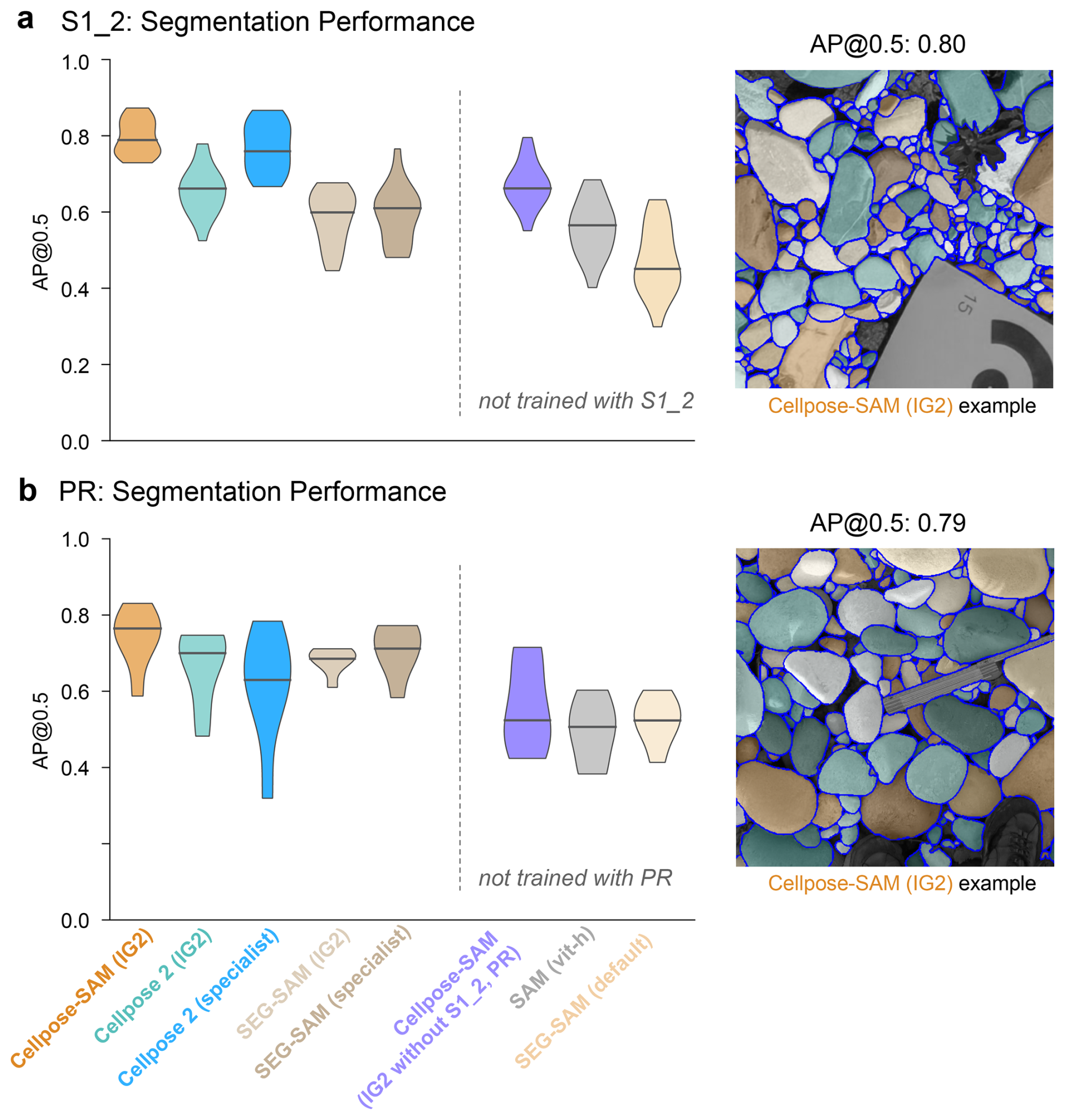
Figure 5 Segmentation results for the S1_2 (a) and the PR (b) subsets. Specialist models were fine-tuned to the respective subset (see Sect. 2 for details). AP@0.5 = average precision evaluated at intersection over union (IoU) threshold of 0.5; SEG-SAM = Segmenteverygrain.

We next evaluated the generalization capability of segmenting grains on image subsets that were not included in the fine-tuning for some model versions, specifically S1_2 and PR (Fig. 5). In this test of how well the model can deal with unseen data, we find that a Cellpose-SAM model trained on all IG2 image tiles except S1_2 and PR outperforms all other methods that were not fine-tuned on these subsets either (Fig. 5a and b). Notably, for both subsets, this model achieves a performance that is comparable to some models that were trained with images from the respective subsets, including both versions of Segmenteverygrain and both versions of Cellpose  2 in PR (Fig. 5a and b). Across both subsets, the overall best-performing model remains Cellpose-SAM that was trained on the full IG2 dataset (Table 2; Fig. 5). However, for S1_2, the older Cellpose  2 architecture trained as a specialist model achieves a performance close to that of the best-performing model (Fig. 5).

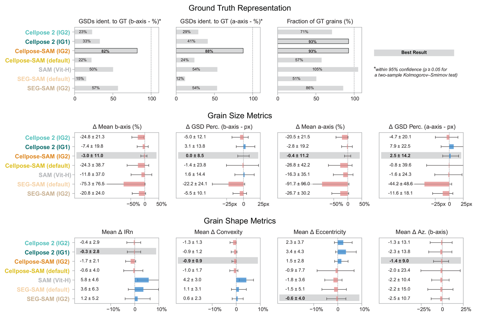
Figure 6 Summary of differences in 2D grain morphometry metrics calculated in relation to manually labelled grain masks (ground truth) across all data subsets. Mean and average standard deviation (1σ) values are calculated for image-averaged values. Values for the best performance in each metric are indicated in bold, while the dashed line indicates perfect representations of the ground truth. GT = ground truth, GSD = grain size distribution, Perc. = percentile, IRn = normalized isoperimetric ratio (IRn, Pokhrel et al., 2024; Quick et al., 2020), Az. = azimuth. SEG-SAM = Segmenteverygrain. For details on individual metrics refer to Sect. 2.2.

3.3 Size and shape accuracy of predicted grains

In a second step, we calculated the same 2D metrics (Fig. 3) for predictions from all evaluated methods and compare them to the respective ground truth image tile. We first evaluate the difference (Δ) between predicted and ground truth ROI masks for each model, aggregated across the full IG2 dataset (Fig. 6). Overall, the predictions derived from our default model (Cellpose-SAM trained on the full IG2 dataset) are the most accurate, showing the closest agreement with the ground truth for 9 out of 11 size and shape metrics (Fig. 6). For the two remaining metrics, mean ΔIR_n and mean ΔEccentricity, our model's predictions are still very similar to the best-performing alternative models (Fig. 6).

In more detail, the total number of detected grains by our default model, Cellpose-SAM (IG2) is also very close to the ground truth, achieving a 93 % recovery rate (Fig. 6). Most notably, mean differences in grain size are around 3 % or below (with ± < 12 % standard deviation for the one sigma range) for both the a- and b-axes, averaged across all detected grains. The resulting grain size distributions (GSDs), based on the lengths of both axes, are statistically identical to the ground truth (within 95 % confidence, p≥ 0.05 for a two-sample Kolmogorov–Smirnov test) in 88 % and 82 % of cases for the a- and b-axes, respectively – compared to 54 % and 57 %, respectively, for the second-best model in this comparison. Our default model also yields the lowest average differences to the percentile values of the GSDs in the ground truth with mean differences of 0 pixels for the b-axis, and 2.5 pixels for the a-axis (Fig. 6). For all shape metrics, the differences between the predicted and ground truth grains are generally relatively small across all models. For our default model, mean Δ values are consistently below 2 % (Fig. 6).

We next examined how the predicted grain masks from our default model compare to the ground truth ROIs across different data subsets. For grain size metrics (mean diameter and percentile differences), most subsets are close to the overall dataset average, with mean Δa- and Δb-axis differences within ± 10 % (Fig. S3 in the Supplement). However, two subsets show a larger variability: AR and NZ2 have average relative differences of −12.4 % and 16.4 % for the a-axis, and −14.6 % and 11.5 % for the b-axis, respectively (Table S3 in the Supplement). A similar variability between subsets is also observed for the average percentile differences in some subsets (Fig. S3, Table S3 in the Supplement). Consequently, the GSDs for both a- and b-axes are statistically identical to the ground truth in five subsets (100 % of image tiles). For another three subsets, the GSDs of both axes are identical to the ground truth in more than 75 % of the image tiles (Table S3). For four of the remaining five subsets, the accuracy of the GSD differs particularly when the lengths of the a- and b-axes are considered separately, with 63 %–100 % of GSDs matching the ground truth. Only subset AR shows a lower agreement where only 50 % of GSDs match the ground truth. Yet this is still comparable to the best results of the second-best performing method and consistent with the average value of the full IG2 dataset (Fig. 6).

Considering grain shape, deviations in the shape metrics, i.e., mean IR_n, mean convexity, mean eccentricity and azimuth, of our default model from the ground truth are generally small. Here, the deviations are less than 5 % (Fig. S3) even in subsets with the largest differences between predictions and ground truth. The only notable exception is the mean IR_n value for DV_4, which deviates by more than 10 % (Fig. S3; Table S3). Finally, the inter-image variability contributes to higher relative standard deviations for several mean difference values in both grain size and shape metrics, resulting in a broader spread in Fig. S3.

4 Discussion

The results show that our IG2 dataset can be used to successfully train and evaluate deep learning models for segmenting individual sediment grains for a broad variety of images taken in a large range of depositional settings (Sect. 4.1). By re-training a state-of-the-art segmentation model (Cellpose-SAM) originally developed for bio-medical research with images of sediment grains, we obtain a model that significantly outperforms other current methods for the same task (Sect. 4.2), despite using the same backbone architecture and starting weights from the Segment Anything Model (SAM). The high-quality segmentation masks generated by our approach allow us to quantify how well grain size and shape are reconstructed relative to the ground truth, which we directly relate to the excellent segmentation performance (Sect. 4.3). Finally, we discuss the limits of our approach and avenues for future development (Sect. 4.4).

4.1 IG2 dataset composition and characteristics

The IG2 dataset was designed to encompass the broadest possible range of grain types (lithology, shape), bedding characteristics (imbrication, fine-material patches), image acquisition conditions (lighting, shadows, brightness), and background elements or non-grain objects (vegetation, scale objects, water bodies). Non-grain objects were excluded from annotation. Where shadows were present, only visible grain boundaries were traced across the shadows. Consequently, the trained Cellpose-SAM model effectively ignores a variety of non-grain features, such as sieves, scales, shoes, ground control point (GCP) markers (e.g., Fig. 5), partial shadows (e.g., Figs. 3 and 4), and vegetation that have previously hampered automated grain detection (e.g., Chan et al., 2026; Miazza et al., 2024; Mair et al., 2022). However, the grain segmentation might only be robust for those objects with shapes, size-ranges, and colors that are similar to those in the training data. Users should also note that grains partially obscured by other objects can introduce biases in quantifying the size and shape of grains, as their reconstructed outlines may deviate from the true boundaries. Yet, this is a problem that is associated with all image-based data collections.

The broad range of imagery and settings yielded a substantial variability of sediment grains with different grain sizes and shapes, with a-axis values ranging from 9 pixels to over 700 pixels (Table S1). This order-of-magnitude range exceeds that of many object-detection tasks and has previously hindered a robust segmentation across the entire size-spectrum (e.g., Chan et al., 2026; Mair et al., 2024). Variations in grain roundness and elongation (Fig. 3, Table S1) surpass those observed along major terrestrial rivers (e.g., Quick et al., 2020; Pokhrel et al., 2024) and even Martian systems (e.g., Szabó et al., 2015). This large range in grain size and shape makes our dataset ideal for evaluating the capability of segmentation models for reconstructions of grain shapes. We emphasize that these ground-truth sizes and shapes are not intended to represent specific geomorphic conditions, but they are rather considered to serve as a benchmark for evaluating the fidelity of model-predicted grain masks on images taken under highly variable conditions (see Sect. 3.2; Fig. 3).

Due to the high variability in grain size, shape as well as general image content and the relatively small number of 243 image tiles, some dataset imbalance persists between training and test splits. Image tiles were carefully selected to minimize this, but divergent segmentation performance in certain cases (e.g., HP; Table S2) suggests the occurrence of some remaining imbalance in specific subsets.

4.2 Capabilities of Cellpose-SAM

4.2.1 Segmentation performance and generalization ability

Our results demonstrate that the high segmentation accuracy achieved by the Cellpose-SAM architecture on biomedical images (Pachitariu et al., 2025) can be effectively transferred to the segmentation of sediment grains. On average, our default model, which was trained on the IG2 dataset, correctly segments a larger number of grains and achieves a higher precision than all benchmark models considered in this study, with an average improvement of ΔAP@0.5 = 0.18 compared to the second-best model (Fig. 4; Table 2). It outperforms both earlier Cellpose  2 models, which employed a U-Net backbone, and workflows that also incorporated SAM, such as SAM itself (ViT-H backbone; Kirillov et al., 2023) and Segmenteverygrain (Sylvester et al., 2025). In contrast, the Cellpose-SAM model not fine-tuned with the IG2 dataset exhibits the lowest performance (Fig. 4), underscoring the effectiveness of re-training and fine-tuning even with comparatively small datasets, such as ours. Notably, training the other benchmark models on the IG2 dataset leads to moderate performance gains for Segmenteverygrain, but to little to no improvement for Cellpose  2 (Fig. 4). This suggests that the default Segmenteverygrain model was originally trained on imagery markedly different from our IG2 dataset, whereas the Cellpose  2 model previously used by Mair et al. (2024) seems to have had already reached its performance limit for images of coarse-grained fluvial sediments. Across the benchmark models used in this study, the median segmentation performances of SAM, the trained Segmenteverygrain, and Cellpose  2 were broadly comparable, with differences mainly at the upper and lower end of the performance distributions. However, these benchmark models did not achieve the same level of segmentation performance as the fine-tuned Cellpose-SAM model (Fig. 4). This outcome aligns with the results of Pachitariu et al. (2025), who demonstrated similar advantages of Cellpose-SAM over other SAM-based architectures (Na et al., 2025; Israel et al., 2024) in biomedical segmentation tasks.

We have evaluated the generalization capability of Cellpose-SAM by training a model that excluded the PR and S1_2 subsets. When compared with Segmenteverygrain and SAM (ViT-H), Cellpose-SAM achieves the highest segmentation performance across both datasets, though with notable differences between them (Fig. 5). For the S1_2 image tiles, the model performs on par with several benchmark models that were explicitly trained on the S1_2 data. In contrast, the model performance for the PR images is more variable, with median AP@0.5 values similar to those of SAM and Segmenteverygrain when these models were not trained with the PR data (Fig. 4). Overall, for the PR tiles, the best-performing model was our default ImageGrains model, which included PR images in its training data.

These results demonstrate the strong generalization capability of Cellpose-SAM, while also indicating that its performance depends, to some extent, on the type of images and on the similarity of the objects of interest and non-grain objects to the data that were used during training. Additionally, our findings show that Cellpose  2 models trained as dataset-specific specialists, i.e., on smaller and more homogeneous image sets, can achieve a segmentation accuracy, which is comparable to, or even exceeding that of the more generalist SAM-based architectures. This was particularly evident for the S1_2 data subset (Fig. 5). Furthermore, our default Cellpose-SAM was the best performing model in all subsets (Table 2) if the data was included in training irrespective of the relative share of the respective subset of the entire IG2 dataset (Table 1). Particularly the performance in subsets with few images of different types (e.g., DV_4, CT) suggests that the inter-subset balance has little effect on the model's generalization ability. We hypothesize that the ability of the SAM architecture to learn a multitude of representation categories, even with class imbalance (Kirillov et al., 2023), is the underlying cause for this performance. Therefore, the deep architecture, combined with the very general initial training of SAM and the two iterations of fine-tuning (first by Pachitariu et al. 2025 and then in our workflow; cf. Fig. 2), should effectively eliminate the need for an inter-subset balance during model training.

4.2.2 3D Segmentation

Data about grain size and shape collected through image-based measurements in 2D have been successfully used to investigate sedimentary systems across a broad range of research (e.g., Garefalakis et al., 2024; Allen et al., 2017; Williams et al., 2013; Marchetti et al., 2022). However, 2D data do not always provide an accurate representation of the size and morphology of grains in 3D (e.g., Garefalakis et al., 2023; Steer et al., 2022; Bunte and Abt, 2001). Consequently, the segmentation of sedimentary grains in 3D remains a critical objective, even though several methodological advancements have been made in recent years to address this challenge (e.g., Domokos et al., 2014; Steer et al., 2022; Walicka and Pfeifer, 2022; Kettler et al., 2023; Rheinwalt et al., 2025). Most of these approaches are designed for segmenting grains from datasets approximating the grains' surfaces in 3D, such as topographic point clouds or meshed grids derived from LiDAR (e.g., Brodu and Lague, 2012) or structure-from-motion (SfM) photogrammetry (e.g., Eltner et al., 2016; Woodget et al., 2018). Grains from such datasets are typically only partially visible due to occlusion (Rheinwalt et al., 2025), which often necessitates the fitting of predefined geometric models during segmentation (e.g., Steer et al., 2022).

In contrast, XR-CT scans can, despite some inherent technical limitations due to scanning contrast and resolution, provide complete volumetric representations of entire grains (e.g., Cnudde and Boone, 2013; Houston et al., 2013; Mitra et al., 2024). These XR-CT data are analogous to the 3D image stacks of microscopic samples used to train and evaluate the 3D-segmentation capabilities of Cellpose (Stringer et al., 2021) and Cellpose-SAM (Pachitariu et al., 2025). Schuster et al. (2026) demonstrated that models with a Cellpose  2 architecture can be successfully trained to segment coarse grains in 3D XR-CT stacks of images taken from glacio-fluvial gravels. In our study, we incorporated the annotated 2D images from Schuster et al. (2026) as subset DV_4, along with annotated micro-XR-CT imagery from Fabbri et al. (2024), to leverage the dedicated 3D capabilities of Cellpose-SAM. We note here that we used these datasets to test the 3D segmentation quality of our default segmentation model and that we refer to cited literature for details on and a discussion of 3D XR-CT scanning itself.

The 3D segmentation of the used example of stacked images yielded 4,647 visually well-defined coarse grains from glacio-fluvial diamictic sediment (Fig. 7). Among all IG2 data subsets, the segmentation performance on the 2D image tiles was highest for DV_4, with a mean AP@0.5 of 0.84, whereas the CT dataset achieved an intermediate performance (Table 2). Notably, for the DV_4 images, the new Cellpose-SAM-based approach produced a net increase in mean AP@0.5 of more than 0.2 compared to the Cellpose  2 model of Schuster et al. (2026). These results indicate that the new default model implemented in ImageGrains 2.0 is well suited for such datasets, with its 3D segmentation capability being particularly promising. It should be noted that, ideally, 3D ground-truth labels would be required to rigorously benchmark the segmentation performance in 3D. However, to our knowledge, the manual effort required to annotate large numbers of image slices in 3D XR-CT stacks has so far impeded the creation of such a reference dataset.

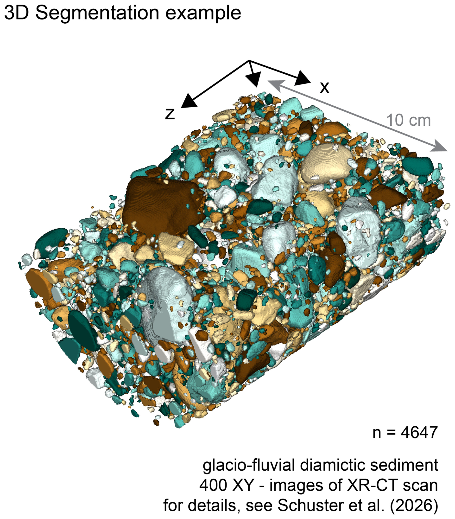
Figure 7 Example where grains were segmented with the default Cellpose-SAM-based segmentation model of ImageGrains 2.0 in 3D from a stack of 400 XR-CT scans taken from of a drill core (drill site 5068_1_C from 4–5 m depth; Schuster et al., 2024) made up of coarse-grained glacio-fluvial sediment.

4.3 Relating size and shape accuracy to segmentation performance

Segmentation-based approaches for measuring grain size and shape have long been limited by inaccuracies arising from over-segmentation, under-segmentation, and imprecise grain boundaries (Chardon et al., 2022; Mair et al., 2022; Steer et al., 2022). The introduction of deep-learning models has substantially improved the accuracy and precision of automated grain segmentation in 2D imagery (Mair et al., 2024; Miazza et al., 2024), with recent developments additionally leveraging the capability of SAM (Chan et al., 2026; Sylvester et al., 2025).

Our new default segmentation model within ImageGrains – a fine-tuned Cellpose-SAM model – further improves both the accuracy and the precision across the entire IG2 dataset, achieving an improvement of up to a 20 % in AP@0.5 and mean average precision (mAP) metrics compared to previous models (Sect. 3.2; Fig. 4). Moreover, the reconstructed grain masks produced by this new default model most closely match the ground-truth ROIs in both size and shape measurements among all benchmark models (Sect. 3.3; Fig. 6). These results confirm the inferences (e.g., Mair et al., 2024) where an improvement in the segmentation performance results in a more accurate quantification of the size and shape of individual grains.

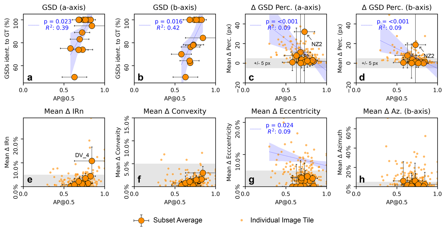
Figure 8 Comparison of segmentation performance metric (AP@0.5) with relative differences in grain size (a–d) and shape (e–h) between predicted grains and the ground truth ROIs for our new default model (Cellpose-SAM IG2). Grey areas indicate very low differences between predicted grain masks and ground truth ROIs, with differences within ± 5 pixels (c, d) and < 5 % (e–h), respectively. Only statistically significant correlations (p≤ 0.05, R²≥ 0.05) for individual images are indicated. For shape metrics (e–h) only values with Δ values > 5 % were considered for correlation. R² = coefficient of determination. Please note that the y-axes in panels (c, d) are cropped for a better visualization of the bulk of results.

Despite this strong overall performance, the model returns results of variable quality across data subsets and individual images (Tables 1 and S4 in the Supplement; Figs. 8 and S2). This variability provides an opportunity to assess how informative the model predictions are for individual size and shape metrics (Fig. 8). In this context, we observe the proportion of predicted grains that are statistically indistinguishable from the ground truth (p≥ 0.05; two-sample Kolmogorov–Smirnov test) to increase significantly with segmentation performance for all data subsets (Fig. 8). We observe similar trends in the results of other tested methods, with an even higher statistical significance due to their generally lower and more variable segmentation performance (Fig. S4 in the Supplement). Although the relatively large number of statistically indistinguishable GSDs prevents the definition of an AP threshold for perfect correspondence, a 100 % match between corresponding GSDs in the ground truth and the predictions is only achieved for cases with average AP@0.5 values exceeding 0.68 (Figs. 8 and S4). For some subsets, higher average AP values do not necessarily yield perfect GSD matches, underscoring the importance of effects related to dataset-specific variabilities; however, no perfect match is achieved below this average AP@0.5 value of 0.68.

This seemingly minimum threshold of 0.68 AP@0.5 IoU (or ca. 0.5 mAP@50-90) for statistically representative GSDs depends on three factors: (i) the specific segmentation results (i.e., whether FP, FN are caused by over/under-segmentation or missed grains), (ii) the grain size sorting, and (iii) the shape of the GSD itself. These factors are interdependent. For example, mis-segmented grains have a much smaller effect on the obtained GSD for a very well sorted sediment with a narrow and Gaussian-shaped GSD than for a poorly sorted sediment with log-shaped or bi-modal GSDs. Therefore, it is unlikely that such a minimum AP threshold exists as an universally applicable value. This implies that efforts to improve the accuracy of the GSD should be directed at improving the segmentation accuracy. This can be achieved through fine-tuning the model to custom annotations and through adhering to classic guidelines for image acquisition. This includes the use of suitable sensors with sufficiently high resolutions, thereby maintaining stable image acquisition conditions (e.g., Bunte and Abt, 2001; Baptista et al., 2012; Bertin and Friedrich, 2016; Purinton and Bookhagen, 2019; Mair et al., 2022).

The average differences between the percentile values of GSDs are generally small, typically < 5 pixels (both a-, and b-axes; Table S3) for a majority of the data subsets and for most individual images (Fig. 8). In general, correlations, where significant, indicate that higher AP@0.5 values are associated with smaller differences in percentile-based GSD metrics relative to the ground truth (Figs. 8 and S3).

For most grain shape metrics, which include roughness (mean IR_n), roundness (mean convexity), elongation (mean eccentricity), and orientation (mean azimuth), the corresponding differences between predicted masks and the ground truths are minor (< 5 % on average) for our default model (Fig. 8; see also Fig. 6 and Table S3), both at the data-subset and individual-image levels. We therefore conclude that segmentation performances with AP@0.5 ≥ 0.6 enable sufficiently accurate and precise reconstructions of the grains' shapes for nearly all images, with only a few outliers (Fig. 8). The other tested methods exhibit larger differences between predicted grain masks and the ground truth, and correlations between segmentation performance and reduced deviations are more frequently detectable (Fig. S4). Overall, the models that were fine-tuned with our IG2 dataset tend to return results that are more reliable in representing the shape than the size of grains.

In summary, the segmentation performance, expressed by AP scores combining false-negative and false-positive detections, correlates with the degree of agreement between predicted and ground-truth grain properties. Therefore, improving the segmentation performance indeed reduces the differences between predicted grain masks and ground truths until they are statistically identical. For our data, our new default model reaches that performance threshold for some data subsets in all metrics (Fig. 8).

4.4 Limitations, applicability, and outlook

4.4.1 Limitations of image-based segmentation

Segmentation-derived grain size and shape data from 2D imagery are widely used across geoscientific disciplines, but the 2D nature of images itself imposes some limits on the applicability of segmentation-based approaches. First, the sizes of grains that can be detected and measured are controlled by the resolution of the image and the content displayed on it. In the IG2 dataset, our default segmentation model applies a filter with a minimum size of 8 pixels for the minor axis of the fitted ellipses. This threshold is close to the technical lower limit of the Cellpose-SAM backbone, which can theoretically detect circular objects with a diameter ≥ 5 pixels (Stringer et al., 2021). The reported lower detection limits for grain segmentation vary considerably among studies, depending on image type and resolution: 6 pixels (Schuster et al., 2026), 12 pixels (Mair et al., 2024), 20 pixels (Chen et al., 2022; Purinton and Bookhagen, 2019), and up to 30 pixels (Chan et al., 2026). At the upper end of the size spectrum, the size of detectable objects is limited by the image extent. By default, Cellpose-SAM detects only objects that are smaller than 40 % of the entire image area (Pachitariu et al., 2025). In addition, although the SAM-based architecture can handle a greater range of size variability than previous models (Pachitariu et al., 2025), an extremely large variability in grain size, i.e., spanning more than an order of magnitude, may require that several masks are combined, which themselves are based on predictions from multiple segmentation runs using differently rescaled images (Chan et al., 2026). We note that the size-limits of objects due to the 2D nature of images always result in truncated GSDs. This effect can complicate comparisons with data collected through other methods, e.g., when comparing grid- or areal-derived GSDs (e.g., Bunte and Abt, 2001; Steer et al., 2022).

Second, our approach is well suited for segmenting objects in 3D in stacked imagery data (see Sect. 4.2.2 above). However, it is not well suited for segmenting objects based on surface data alone or incomplete 3D representations of grains, such as those obtained from topographic point clouds. Therefore, they require a geometric extrapolation to segment those grains successfully (Steer et al., 2022; Rheinwalt et al., 2025).

Third, some limitations arise from image type and content. While modern deep-learning models, particularly Cellpose-SAM, can be applied to a broad variety of imagery because of the strong capability for generalization (Pachitariu et al., 2025; see also Sect. 4.2.1), the segmentation can be hampered, and, thus, the performance be limited due to the occurrence of complex contents in the imagery itself. Examples include unrelated objects or vegetation, challenging lighting conditions (e.g., shadows, reflections, or glare from water bodies), motion blur, and color imbalance. To counter these effects, we composed the IG2 dataset with images encompassing a broad range of conditions at which the images were taken, thereby enhancing the model's robustness. Consequently, our default model is able to handle a variety of adverse imagery conditions and unrelated objects effectively. However, due to the finite size of the dataset, the performance may decline when applied to imagery that substantially differs from the contents represented in the IG2 dataset. Examples of such differences include objects that are very different from clasts (such as human-made objects), images taken in very different vegetation zones and on other planets, or entirely new types of imagery such as images of thin sections. In such cases, fine-tuning with a small number of additional training tiles (as few as seven or fewer) can yield substantial improvements, as demonstrated for the CT, HP and FH_2 data splits (Table 1). Here, the combination of a deep transformer architecture with SAM's generalist encoder weights effectively reduces the need for extensive dataset balancing, which was essential for earlier, shallower architectures (e.g., Mair et al., 2024).

Finally, an insufficient segmentation performance likely poses the major limiting factor for some applications. The definition of an exact threshold that constitutes a sufficient level of segmentation performance remains an application- and dataset-specific task (see Sect. 4.3; Zaidi et al., 2022). In case of insufficient segmentation (over- or under-segmentation, as well as missed grains), a manual post-processing, i.e., correcting the mis-segmented grains, is recommended. This could be done through the graphical user interface or any software tool that allows the creation and modification of mask ROIs.

4.4.2 Hardware requirements and environmental costs

Cellpose-SAM and similar transformer-based architectures require considerably more computational resources and dedicated GPU support than earlier, shallower segmentation models, both during training and inference. Nonetheless, training a Cellpose-SAM model is feasible on a standard desktop equipped with a mid-range GPU, such as an NVIDIA GeForce RTX 3070 with 8 GB of RAM. Under this configuration, training with our dataset required more than 40 h, compared to < 1.5 h on an NVIDIA A100 GPU with 80 GB of memory (see Sect. 2.3 for details). For inference, dedicated GPUs (e.g., NVIDIA or Apple M2 and newer chips) with at least 3 GB of RAM are required to segment large images (> 1000 pixel × 1000 pixel) within a few seconds. Detailed performance benchmarks are provided in Pachitariu et al. (2025; Tables S2 and S3). Measurements of grain size and shape in ImageGrains operate at comparable speeds, enabling the automated analysis of thousands of grains within minutes.

Recent increases in the depth of models and the sizes of training data for deep learning led to a large increase of computational resources that consume substantial amounts of energy, which exerts a high toll on the environment (e.g., Strubell et al., 2019; van Wynsberghe, 2021). It is difficult to precisely quantify the environmental costs of such models due to the question of how to factor in the initial training of SAM (which is reported to have cost c. 6963 kWh or equivalent to 2.8 t of CO₂ released; Kirillov et al. 2023), and the open question of how to account for secondary effects beyond the computational cost and energy consumption (e.g., Yu et al., 2024; Bouza et al., 2023). Furthermore, quantifying the environmental impact of energy consumption for training or inference requires dedicated tests and often-unavailable information, such as where a specific piece of hardware was used and what energy source powered it (e.g., Lacoste et al., 2019; Patterson et al., 2021; Jay et al., 2023). However, we can estimate the computational cost (and therefore the energy cost) of our approach, based on the results of Pachitariu et al. (2025; cf. Tables S2 and S3 therein). We note that the Cellpose-SAM architecture runs on local desktop computers with mid-range consumer hardware configurations (see above), both for inference and for retraining smaller models (not more than a few hundred images). Therefore, despite the rather costly initial training and release of SAM (Kirillov et al., 2023), using or fine-tuning our model in ImageGrains has a comparatively small computational cost and thus a low environmental impact, comparable to running any other software for similar durations on a desktop PC.

Finally, the ImageGrains library is distributed as an installable Python package, allowing both local and cloud-based deployment across platforms (see code availability section below). This enables efficient execution even on free online platforms, such as Google Colab, for users without access to suitable local hardware.

4.4.3 Applicability

The introduction of a fine-tuned Cellpose-SAM model as the default segmentation engine in the ImageGrains 2.0 library significantly enhances the performance of segmenting grains relative to previous versions (Mair et al., 2024). This improvement benefits not only the direct applications of this workflow (e.g., Patel et al., 2025; Rezwan et al., 2025; Zegers et al., 2025) but also a broad range of applications that rely on the segmentation of grains in coarse-grained fluvial sediments, especially when high accuracy is required across large areas (e.g., Guerit et al., 2018; Purinton and Bookhagen, 2021; Marchetti et al., 2022). This is particularly the case when grain size accuracy had previously been a challenge (e.g., Chardon et al., 2022; Miazza et al., 2024), or when the spatial variability in grain size is high (e.g., Rice and Church, 1998; Guerit et al., 2014). The expanded IG2 dataset enables the application of our default model to additional sedimentary contexts, such as XR-CT imagery of glacio-fluvial clasts (Schuster et al., 2026), bioclastic marine sands (e.g., Fabbri et al., 2024) and proglacial angular sediments (e.g., Hiller et al., 2023). For CT-based image stacks, the segmentation can be extended to fully capture the 3D nature of sediment grains. The high precision of the predicted grain masks allows for a robust analysis of the shape of grains, with the metrics used in this study provided as default outputs in ImageGrains. Furthermore, the availability of individual 2D grain masks as output enables the analysis of shapes tailored and customized to specific research requirements. Moreover, the high segmentation performance and generalization capability enable robust and precise segmentation of sediment grains in images of sediment other than coarse, clastic material. Our workflow should be adaptable, with minimal annotation effort, for similar segmentation tasks of other types of sediment (e.g., Dawson et al., 2025; Mitra et al., 2024; Liu et al., 2024), or even for segmenting other image-based objects that are of geoscientific relevance (e.g., Hsiang et al., 2019; Kloster et al., 2023). In general, the approach can be generalized to any category of segmentable objects in geoscientific imagery, where dense segmentation is needed to create ROI-based outputs for object morphometry. Such outputs could then be used as inputs for other machine learning tasks, e.g., for classification tasks. Furthermore, our publicly available dataset can be used in combination with own labels for fine-tuning to other image types and settings. Finally, the manually annotated masks for individual grains can be used to train and test other segmentation approaches.

4.4.4 Future directions

This study demonstrates that state-of-the-art deep learning models originally developed for biomedical image segmentation can be successfully adapted for segmenting sediment grains. Similar to the segmentation of biomedical images, domain-specific architectures optimized for grain imagery outperform generic computer vision approaches, despite sharing foundational components such as SAM encoders and pre-trained weights (see Sect. 4.2.1). This suggests that the same underlying principles apply for these tasks.

However, a notable difference between the two application domains lies in absolute performance of the segmentation. The median AP@0.5 for our full IG2 dataset (0.72) is lower than that reported for Cellpose-SAM on the Cellpose biomedical dataset (> 0.85; Pachitariu et al., 2025). We attribute this difference primarily to the smaller size of the IG2 dataset (243 image tiles compared to over 1000 microscopy images in the Cellpose nuclei dataset), the greater variability of the imagery regarding the size distribution and texture of the grains displayed in this imagery, and the conditions at which they were taken in the field. This interpretation is supported by the variable model performance across IG2 subsets, which correlates with grain size accuracy, and to a lesser extent, with grain shape accuracy (Fig. 8; Table S3). Thus, future improvements in measuring the size and shape of grains will depend strongly on enhancing the performance of segmenting grains.

Progress in this direction is likely to come from the creation of larger and more variable annotated datasets and from the adoption of standardized image acquisition protocols that reduce the variability in image content. Given the effort of labelling/annotating large amounts of images and the fact that only a handful of annotated images are required for fine tuning the model, we expect that these larger and more variable datasets will be compiled from a collection of smaller datasets from different studies, if published by the community (e.g., Saddi et al., 2026). Moreover, obtaining annotations from multiple experts for the same images would enable calculation of values reflecting an inter-annotator consensus-level, a common benchmark for assessing absolute segmentation quality in other fields (e.g., Braylan et al., 2022; Yang et al., 2023; Zhou et al., 2025). Current SAM-based segmentation models appear capable of achieving such inter-annotator consensus–level accuracy for 2D images when trained on suitable datasets (Pachitariu et al., 2025; Na et al., 2025; Israel et al., 2025). This suggests that future advances in grain size and shape measurement will be driven less by architectural refinements but more by the development of larger and representative training datasets of high quality.

5 Conclusions

We present a collection of 243 manually annotated images of sediment, the IG2 dataset, designed to enable systematic assessment and training of deep-learning architectures for segmenting sediment grains. Furthermore, we introduce ImageGrains 2.0, an updated open-source framework for automated measurement of grain size and shape that integrates Cellpose-SAM as a fine-tuned default segmentation model for this task. Across the IG2 dataset, the model improves segmentation performance by up to 20 % in AP@0.5 and mAP compared to selected benchmark workflows, yielding grain masks that most closely match the ground-truth regions of interest for both size and shape metrics. The model's strong generalization capability enables accurate segmentation across multiple image types and settings, including XR-CT imagery, and across variable grain textures and imaging conditions. The segmentation performance correlates directly with the accuracy of the derived grain size and shape metrics, confirming that improved segmentation performance translates to more robust geomorphic measurements. Additionally, the model can be fine-tuned with only a few additional image tiles to adapt to new sediment types or imaging conditions, making it applicable for a broad range of applications.