the Creative Commons Attribution 4.0 License.
the Creative Commons Attribution 4.0 License.
 | 29 May 2019
Determining the optimal grid resolution for topographic analysis on an airborne lidar dataset
Aljoscha Rheinwalt
Bodo Bookhagen
Digital elevation models (DEMs) are a gridded representation of the surface of the Earth and typically contain uncertainties due to data collection and processing. Slope and aspect estimates on a DEM contain errors and uncertainties inherited from the representation of a continuous surface as a grid (referred to as truncation error; TE) and from any DEM uncertainty. We analyze in detail the impacts of TE and propagated elevation uncertainty (PEU) on slope and aspect.
Using synthetic data as a control, we define functions to quantify both TE and PEU for arbitrary grids. We then develop a quality metric which captures the combined impact of both TE and PEU on the calculation of topographic metrics. Our quality metric allows us to examine the spatial patterns of error and uncertainty in topographic metrics and to compare calculations on DEMs of different sizes and accuracies.
Using lidar data with point density of ∼10 pts m−2 covering Santa Cruz Island in southern California, we are able to generate DEMs and uncertainty estimates at several grid resolutions. Slope (aspect) errors on the 1 m dataset are on average 0.3∘ (0.9∘) from TE and 5.5∘ (14.5∘) from PEU. We calculate an optimal DEM resolution for our SCI lidar dataset of 4 m that minimizes the error bounds on topographic metric calculations due to the combined influence of TE and PEU for both slope and aspect calculations over the entire SCI. Average slope (aspect) errors from the 4 m DEM are 0.25∘ (0.75∘) from TE and 5∘ (12.5∘) from PEU. While the smallest grid resolution possible from the high-density SCI lidar is not necessarily optimal for calculating topographic metrics, high point-density data are essential for measuring DEM uncertainty across a range of resolutions.
- Article
(8416 KB) - Full-text XML
-
Supplement
(34573 KB) - BibTeX
- EndNote


Continuous surfaces are often projected onto an evenly sampled grid – digital elevation models (DEMs) are a common example. The accuracy of the gridded representation of the underlying surface is controlled by the spacing of the grid, the variability of the surface (i.e., the terrain itself), and the amount of uncertainty added during data collection and processing.
In recent years, an ever-growing array of DEM datasets has become available across a range of resolutions and spatial scales. As new data acquisition and processing strategies – such as lidar, stereo photogrammetry, and structure from motion – mature, the number and variability of features represented in a DEM will grow dramatically. In this paper, we refer to DEMs as high resolution when their grid spacing is low (e.g., 1–3 m) and low resolution when their grid spacing is high (e.g., a 10+ m DEM). Across all DEM resolutions, it is important to quantify the uncertainties in DEMs and their potentially large impacts on metrics calculated from the DEM (Florinsky, 1998; Zhou and Liu, 2004; Oksanen and Sarjakoski, 2005; Wechsler and Kroll, 2006; Wechsler, 2007).
The estimation of topographic metrics, such as slope and aspect, is a common task across scientific disciplines. Slope and aspect provide important boundary conditions for hillslope stability analysis (e.g., Montgomery and Dietrich, 1994; Tucker and Bras, 1998) and landslide monitoring (e.g., Guzzetti et al., 1999; Ayalew and Yamagishi, 2005), geomorphic transport laws (e.g., Roering et al., 1999; Dietrich et al., 2003; Pelletier, 2008; Grieve et al., 2016), hydrologic applications (e.g., Band, 1986; Zhang and Montgomery, 1994; Tarboton, 1997; Pelletier, 2010, 2013) including flood risk modeling (e.g., Ouma and Tateishi, 2014) and stream power analysis (e.g., Bookhagen and Strecker, 2012; Lague, 2014), tectono-geomorphic modeling (e.g., Whipple and Tucker, 1999; Snyder et al., 2000; Tucker and Hancock, 2010; Kirby and Whipple, 2012; Bookhagen and Strecker, 2012), ecologic modeling (e.g., Franklin, 1995; Guisan and Zimmermann, 2000; Thompson et al., 2001), and vegetation analysis (e.g., Pierce et al., 2005; Kent, 2011).
A wide range of methods has been developed to accurately derive slope and aspect from elevation data using a range of approaches, each optimized for different use cases (e.g., Evans, 1980; Zevenbergen and Thorne, 1987; Skidmore, 1989; Tarboton, 1997; Dunn and Hickey, 1998; Schmidt et al., 2003). For example, the methods D-8 and D-infinity are optimized towards hydrologic flow-routing problems, particularly on DEMs of low spatial resolution (Tarboton, 1997), and the methods of Evans (1980) and Zevenbergen and Thorne (1987) include some smoothing of the underlying DEM to minimize the impacts of DEM noise. However, all of these methods contain some intrinsic error due to truncation error (TE) – the deviation of the gridded sample from the continuous original surface (Fig. 1). The TE describes the error made by truncating an infinite sum and approximating it by a finite sum. It often includes a discretization error, which arises from taking a finite number of steps to approximate a continuous surface. Several authors have explored the theoretical limitations of estimations of slope and aspect calculations on gridded surfaces (e.g., Heuvelink et al., 1989; Hunter and Goodchild, 1997; Florinsky, 1998; Abarbanel et al., 2000; Zhou and Liu, 2004); in general, TE can be related directly to the grid sampling – more tightly sampled grids will deviate less from the original surface.
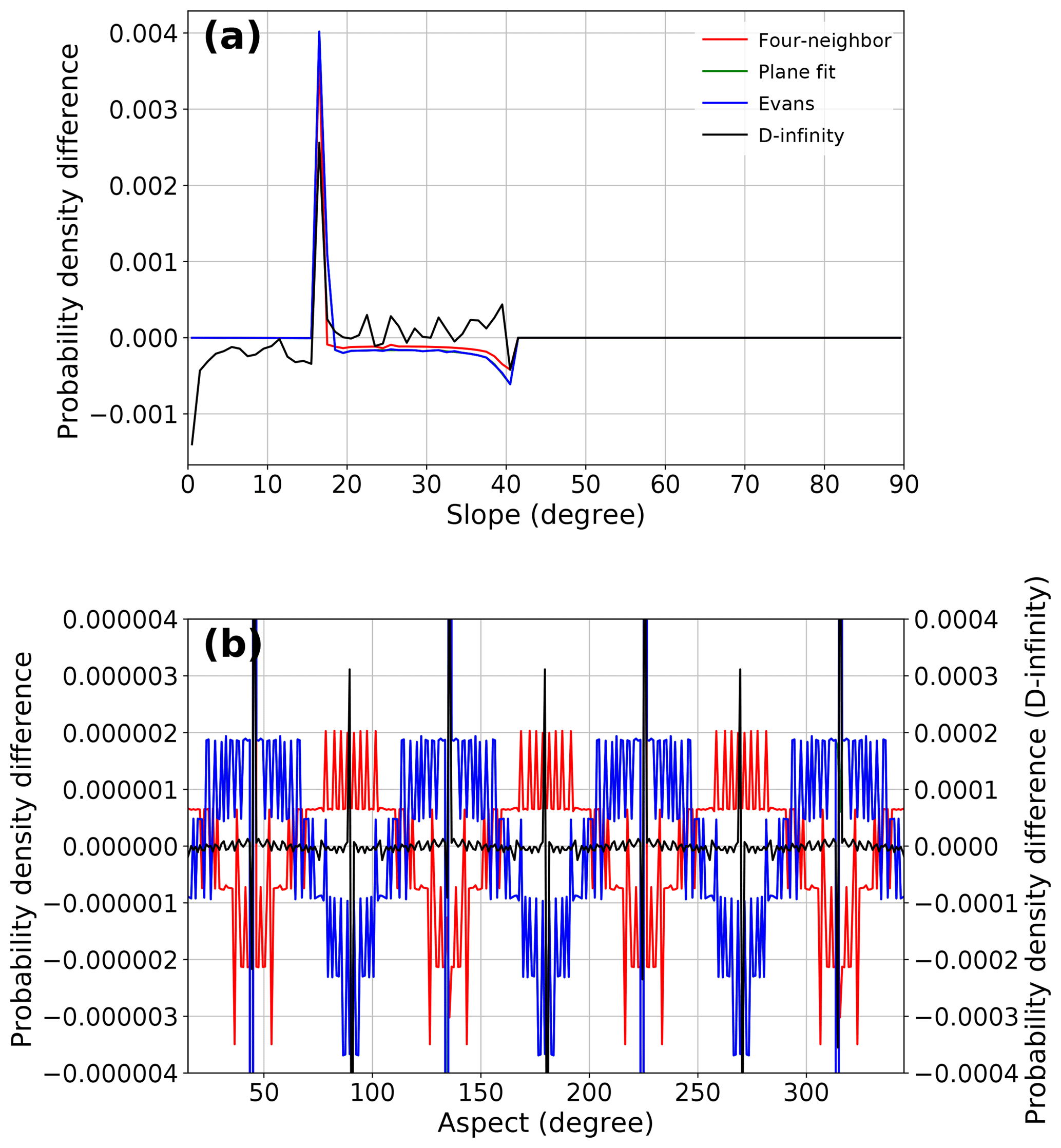
Figure 1(a) Slope and (b) aspect distribution differences from analytical solutions of slope and aspect on a Gaussian hill, on 1∘ bins, starting from [0.5, 1.5). None of the methods perfectly match the analytical solution, with slightly different offset magnitudes. Note that the D-infinity method (black line) produces aspect frequency distribution errors 2 orders of magnitude larger than those errors produced by the other methods. It is important to note, however, that the aspect offsets are small – on the order of 1–5 pixels per bin for the methods excluding D-infinity.
In addition to TE, real-world DEMs will have some degree of measurement uncertainty. The magnitude of that uncertainty varies across data collection methods and data post-processing but also depends on the terrain itself and is often difficult to estimate (Heuvelink et al., 1989; Lee et al., 1992; Bolstad and Stowe, 1994; Florinsky, 1998; Fisher, 1999; Smith and Sandwell, 2003; Farr et al., 2007; Wechsler and Kroll, 2006; Wechsler, 2007; Mukul et al., 2017; Purinton and Bookhagen, 2017, 2018; Wessel et al., 2018). Any uncertainty in elevation estimates will propagate into the calculated topographic metrics.
The impacts of TE and DEM uncertainty on slope and aspect estimations can be quantified for any gridded data. We first use synthetic data with known properties as a control to define generalized functions applicable to any DEM and to develop a quality metric for slope and aspect calculations. Following this analysis, we turn to a high-resolution lidar dataset covering complex terrain to study the spatial structure of uncertainty in topographic metrics propagating from both TE and DEM uncertainty. This novel approach allows us to identify the optimal grid resolution that minimizes the error bounds from the combination of TE and PEU, and to analyze the implications of using suboptimal DEM resolutions for calculating slope and aspect.
In this analysis, we demonstrate the limitations of calculating slope and aspect using synthetic data surfaces. These surfaces serve as a valuable control dataset, as the precise analytical values for slope and aspect at each grid cell are known. We further add normally distributed random noise with a known mean and standard deviation to our synthetic data to investigate the impacts of DEM uncertainty on topographic metrics. Following the discussion of synthetic data, we apply the same methods to high-resolution lidar data interpolated to DEMs with varying spatial resolutions.
2.1 Synthetic data
We generate regular n×n grids of size n=11, 101, and 1001 describing a Gaussian hill with a maximum height of 1, with elevations defined on a regular square grid as for each (x,y) grid cell (Fig. 2). A second surface describing a sphere is included in the Supplement. It is important to note that the horizontal and vertical units for the synthetic data are arbitrary – the grid cell spacings generated by using differently sized grids are an expression of the width-to-height ratio of the surface. The Python functions used to generate our synthetic surfaces can be found on GitHub: https://github.com/UP-RS-ESP/TopoMetricUncertainty/blob/master/surfaces.py (last access: 17 May 2019).

Figure 2Gaussian hill elevations at n=11, 101, and 1001. As grid sizes increase, a smoother surface is generated. Note that the horizontal and vertical units are arbitrary and that the grid cell spacings are an expression of the width-to-height ratio of the surface. Cross sections of the shapes at all grid sizes can be seen in Fig. S1.
2.2 Topographic metrics
In this study, we focus on the topographic metrics (1) slope (S(x,y)) and (2) aspect (A(x,y)) which we define as
and
with x and y being the spatial coordinates. Key in calculating slope and aspect is the calculation of the directional derivatives and .
There exists a wide range of methods for calculating the directional derivatives on gridded data that broadly fall into three classes: (1) four-neighborhood methods, (2) eight-neighborhood methods, and (3) steepest descent methods (e.g., Evans, 1980; Zevenbergen and Thorne, 1987; Skidmore, 1989; Tarboton, 1997; Dunn and Hickey, 1998; Schmidt et al., 2003; Zhou and Liu, 2004; Oksanen and Sarjakoski, 2005). In our analysis, we use the standard second-order finite difference approximation as implemented in Python NumPy (Fornberg, 1988; Durran, 1999), which is a four-neighborhood method. We tested additional methods using eight neighborhoods (e.g., singular-value decomposition plane fitting and the method of Evans, 1980) – which provide some underlying DEM smoothing and are well suited to noisy DEM data – and using steepest descent (e.g., D-8 and D-infinity; Tarboton, 1997), which identify the steepest slope that water would take and are optimized for hydrologic use cases. However, these methods do not necessarily provide the most representative slope of the terrain and show distinct differences from the analytical solutions of slope and aspect (see Figs. S2 and S3 in the Supplement). We choose to use the simple four-neighbor method in our analysis, as it results in the lowest relative error when compared with the analytical solution for slope and aspect (Fig. S2) and does not include any smoothing of the underlying DEM.
Biases in topographic metrics can be determined both numerically, by comparing the results of calculations to known values, and analytically, by deriving the impacts of both TE and DEM uncertainty on topographic metrics.
3.1 Truncation error
We derive the TE from the formulas of topographic metrics by propagating the uncertainty of the second-order finite difference approximation for the directional derivatives and . Neglecting rounding errors, we assume the uncertainty ε of the second-order finite difference Δ to be bounded by
where a represents either x or y, and h is the grid spacing.
The considered topographic metrics – slope (S(x,y)) and aspect (A(x,y)) – depend on both directional derivatives and . As the corresponding uncertainties εx and εy are not independent, propagated TE T for slope (TS) and aspect (TA) are given by
These can be more explicitly expressed using Eq. (3) as
The sign of the TE is derived from symmetry considerations in the following way:
and
Equations (6)–(9) allow us to calculate the magnitude of the TE at each point (x,y) on our synthetic surfaces (Fig. 3).
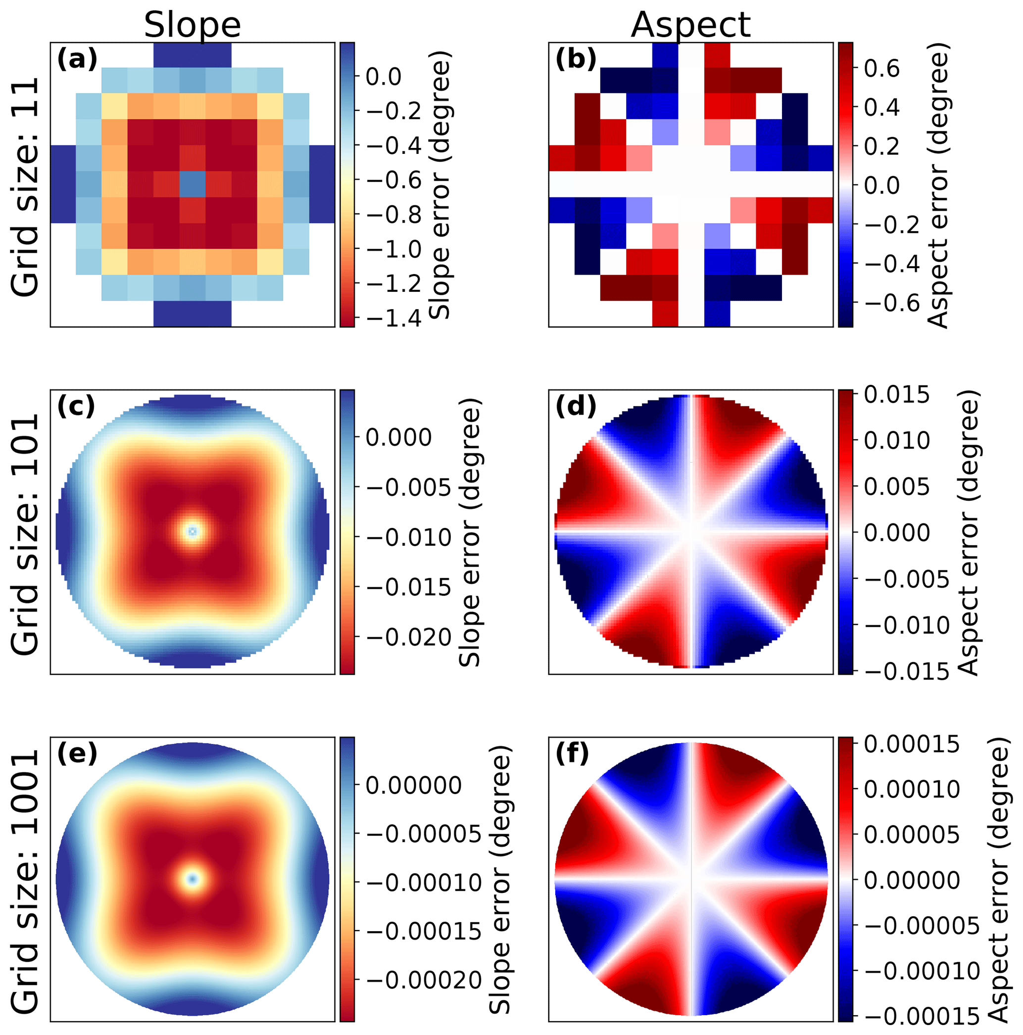
Figure 3Gaussian hill slope (a, c, e) and aspect (b, d, f) errors from the analytical TE. All grid sizes show clear spatial patterns in slope and aspect errors. Offset magnitudes scale with grid size. Errors on the n=1001 grid (e, f) are generally 2 orders of magnitude smaller than those for the n=101 grid (c, d). Colors are scaled from the 5th to 95th percentiles of error magnitudes.
As can be seen in Fig. 3, the magnitude of the slope and aspect error decreases with increasing n. This implies that as more tightly sampled models of a surface are used, the accuracy of slope and aspect estimations increases. This follows the work of Abarbanel et al. (2000), which shows that finite difference derivative estimations have error magnitudes that scale with the inverse of the grid spacing for evenly spaced grids. However, even with increasingly accurate surface models, there remains some TE simply due to the fact that a smooth surface cannot be perfectly represented by gridded data. At very fine scales, computer rounding will also lead to errors in slope and aspect calculations. In this study, however, we do not use fine enough grids for this to impact our error estimates.
As the precise mathematical definitions of our synthetic surfaces are known, we can analytically derive their slope and aspect values at each point and compare those results to numerical calculations (see Fig. S4). In the absence of DEM uncertainty, the difference between analytically and numerically derived topographic metrics will be dominated by the TE from the second-order finite difference approximation. Additionally, modifying the absolute magnitude of the shape heights (e.g., a maximum height of 100 instead of 1) does not modify the absolute magnitudes of slope and aspect TE (see Fig. S5).
Slope and aspect calculations have very different spatial error patterns (see Fig. 3). However, as with aspect errors, slope errors depend on the orientation of the grid despite the radial symmetry of the surface. This is easiest to see in the slope difference map of the Gaussian hill, where error magnitudes are not simply scaled by slope (see Fig. 3e).
3.2 DEM uncertainty
Elevation models are never perfect – there are always errors and uncertainties due to data collection or processing. The uncertainty in calculated topographic metrics can be constrained by propagating DEM uncertainties into their calculations (e.g., Heuvelink et al., 1989; Hunter and Goodchild, 1997; Zhou and Liu, 2004; Oksanen and Sarjakoski, 2005); we refer to the uncertainty introduced into slope and aspect calculations from elevation uncertainty as propagated elevation uncertainty (PEU). For our synthetic data, we assume the simplistic but straightforward error model of spatially uncorrelated white noise. We define noise to be normally distributed and consider two cases: (1) homogeneous white noise, i.e., noise drawn from one unique normal distribution , and (2) slope dependent, spatially varying white noise, i.e., noise drawn from a family of normal distributions . Since for each grid cell noise is drawn independently, the PEU for slope (ES) and aspect (EA) is given by
As before, this can be expressed more explicitly using Eq. (3) as
As with TE, PEU introduces distinctive spatial patterns into the slope and aspect estimates (Fig. 4). Both slope and aspect uncertainties are higher on shallow slopes, as has been shown in previous work (Florinsky, 1998; Zhou and Liu, 2004). On flat or nearly flat terrain, the elevation uncertainty will more strongly impact the estimated partial derivatives and thus lead to erroneous slope and aspect estimates. It is also important to note that aspect varies between [0, 360) and slope only between [0, 90), which is why we expect standard deviations to be different by a factor of 4 (see Fig. 4).
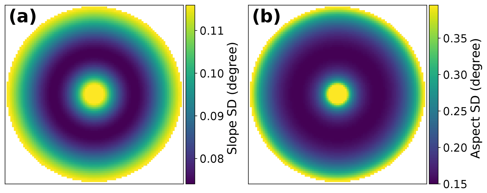
Figure 4Gaussian hill (n=101) slope and aspect standard deviations for spatially invariant noise (SD ), derived from elevation uncertainty propagation (Eqs. 12–13). Aspect has higher standard deviations than slope, as aspect varies between [0, 360) and slope only between [0, 90). This is evident especially on flat terrain (e.g., the edges of the Gaussian hill).
When we compare our analytically derived topographic metric uncertainty patterns (Fig. 4) to those generated from actual random noise – using an ensemble of 10 000 synthetic surfaces, each generated with normally distributed noise – the spatial patterns and magnitudes are nearly identical between the two methods (see Fig. S6).
Both TE and PEU yield distinct spatial patterns, implying that the error and uncertainty in topographic metrics will vary throughout a DEM. Using both the TE and PEU magnitudes, we can examine whether TE or PEU is dominant at an arbitrary grid spacing, given a known DEM uncertainty (Fig. 5).

Figure 5TE and PEU magnitudes for two noise levels, (a) 1e−4 and (b) 1e−6, compared to grid spacing. Aspect is plotted in black; slope is plotted in gray. Solid lines are used for PEU; dashed lines are used for TE. TE decreases with decreasing grid spacing, while PEU increases as the noise standard deviation relative to grid spacing increases.
As can be seen in Fig. 5, TE will approach zero for sufficiently small grid spacings, while PEU will rise as the amount of noise relative to the grid spacing increases. Using both TE and PEU magnitudes across grid spacings, an optimal grid spacing for a given noise level which minimizes their combined influence can be chosen. Note that we do not assume that the quality of the data is maximized when the combination of TE and PEU is minimized, but that the error bounds on topographic metric calculations are minimized. Thus, the optimal grid spacing is preferred for calculating slopes and aspects for use in applications where uncertainty across the entire grid should be minimized.
4.1 Metric quality ratios
The trade-off between TE and PEU can also be thought of as a quality ratio. Simply put, the impact of DEM uncertainty on topographic metrics is modulated by the grid spacing – i.e., 1 cm of vertical noise on a 10 m grid will have a very different impact than 1 cm of vertical noise on a 1 cm grid. As both TE and PEU have distinct spatial patterns, a combined quality ratio (QR) can capture a holistic view of the overlapping influence of TE and PEU. The QR can be defined from the combination of the TE and PEU as
where m is a normalization factor which accounts for the 4-fold difference in the range of possible values between slope and aspect. On a surface without noise, the QR will approach 1 as grid spacing and TE approach 0. The influence of TE and PEU on calculated QRs can be seen by comparing the same synthetic grid with two noise levels (see Fig. S7). High noise levels reveal similar spatial patterns to those seen in Fig. 4, while low noise levels show the influence of TE (see Fig. 3).
The QR can also used as a normalized metric to compare DEMs across grid spacings and noise levels (Figs. 6 and S8). Each noise level/grid spacing pair has a point at which the QR of the DEM is maximized. This point represents the optimal trade-off between TE and PEU over the entire grid.
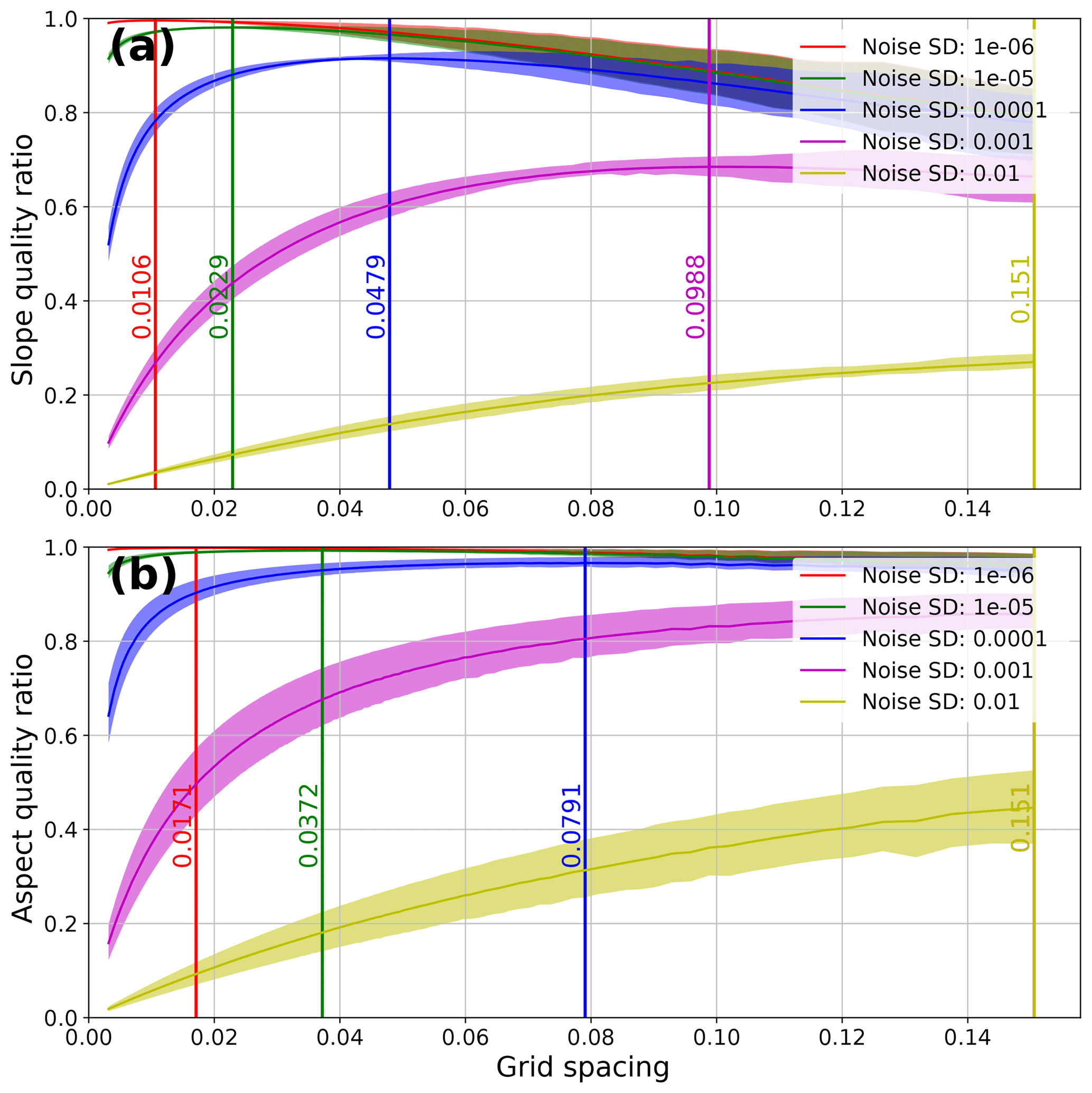
Figure 6Gaussian hill slope (a) and aspect (b) QRs vs. grid spacings for a range of noise levels (1e−2 to 1e−6). The 25th–75th percentile QRs are shaded for each noise level. Optimal grid spacings (maximum QR) for each noise level are marked with vertical lines. Slope calculations result in lower optimal grid spacings compared to aspect. Higher noise levels lead to higher optimal grid spacings for both slope and aspect calculations. Note that the purple and yellow lines in panel (b) have the same optimal grid spacing, and thus only the yellow line is visible.
As can be seen in Fig. 6, as noise levels increase, the optimal grid spacing increases, and the QR of that optimal spacing decreases. For very noisy datasets (purple and yellow lines; Fig. 6), very large grid cell spacings – i.e., aggregation – can help reduce the combined influence of TE and PEU on slope and aspect estimates.
There are distinct differences between the optimal slope and aspect grid spacings for the same dataset. For any given noise level, the optimal grid spacing to calculate aspect is higher than that for slope. The difference in optimal grid spacing is driven by the relative magnitudes of the PEU between slope and aspect calculations – the PEU for aspect calculations is always higher than that for slope due to differences in the formulas for slope and aspect (see Fig. 5 and Eqs. 12–13).
4.2 Heterogeneous noise
In practice, datasets will not have homogeneous noise across grid spacings – coarser parameterizations of a surface will include more uncertainty as fine-scale features are aggregated into single pixels. Additionally, noise in real-world datasets is influenced by non-uniform landscape features such as slope, aspect, terrain relief, and vegetation cover (e.g., Kraus and Pfeifer, 1998; Kyriakidis et al., 1999; Holmes et al., 2000; Smith and Sandwell, 2003; Carlisle, 2005; Oksanen and Sarjakoski, 2006; Rodriguez et al., 2006; Shortridge and Messina, 2011; Purinton and Bookhagen, 2017; Purinton and Bookhagen, 2018). While several authors (e.g., Hunter and Goodchild, 1997; Zhang and Goodchild, 2002; Fisher and Tate, 2006) have examined complex error models in real data, we choose to use a simplistic error model based on terrain slope – e.g., higher slopes have higher noise levels – to look at the first-order impacts of heterogeneous noise on the calculation of topographic metrics.
When we compare the heterogeneous noise result to the analysis shown in Fig. 6 (see Fig. S9), the results are very similar, albeit with higher optimal grid spacings. We can also compare the optimal grid spacings for homogeneous and heterogeneous noise directly for a set of noise levels from 1e−8 to 1e−2 (Fig. 7).
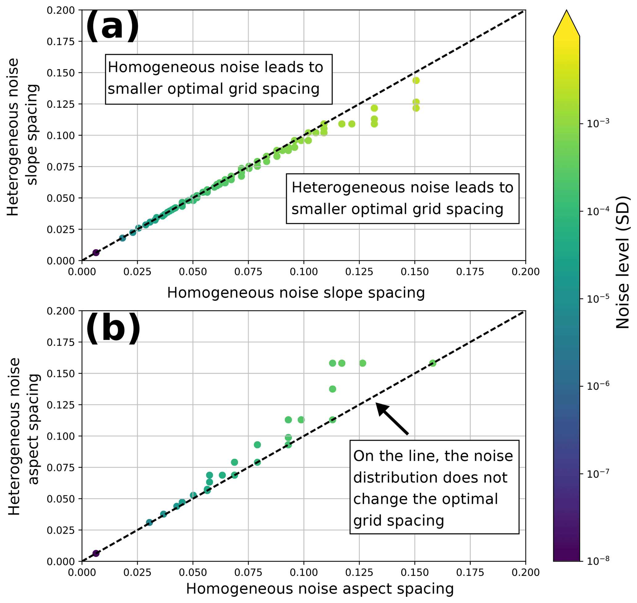
Figure 7Optimal grid spacing for slope (a) and aspect (b) across a range of noise levels (1e−2 to 1e−8). Points in the upper triangle have smaller optimal grid spacings with homogeneous noise. Points in the lower triangle have smaller optimal grid spacings with heterogeneous noise. Points on the dashed line have the same optimal grid spacings regardless of the noise distribution. Heterogeneous noise leads to smaller slope grid spacings but larger aspect spacings for the same average noise level.
As can be seen from Fig. 7, slope can be calculated on a smaller grid spacing with slope-biased noise, while aspect should be calculated with a larger grid spacing. The divergence in the optimal grid spacings between homogeneous and heterogeneous noise is driven by the differences in the influence of terrain slope on slope and aspect QRs. While both slope and aspect calculations have similar grid-spacing-dependent TE magnitudes, the differences in the relative magnitudes of the PEU lead to different responses to the distribution of noise on the DEM (see Fig. 5). The simplistic slope-dependent error model used here is unlikely to translate to a real-world setting; however, it is clear that the spatial distribution of noise on the DEM influences the choice of optimal grid spacing for both slope and aspect calculations.
As can be seen in Figs. 4–6, the introduction of noise has non-trivial impacts on slope and aspect calculations. To examine the impact of both TE and PEU on the frequency distributions of slope and aspect, we generate 1000 member ensembles of slope and aspect for each combination of two different grid sizes (n=101, 1001) and three different noise levels (homogeneous noise, SD , 1e−3, 1e−4). We then bin the ensemble data into 1∘ slope and aspect bins.
When homogeneous noise is added to synthetic surfaces, the large spikes in aspect distributions related to the cardinal directions (e.g., at 45/90/135∘) are smoothed out into neighboring bins. However, this does not imply that the calculated aspects are “better”, just that they have a more even distribution – the PEU overprints the TE as seen in Fig. 3. This can clearly be seen in Fig. S10, which shows the impact of noise on slope and aspect grids.
Slope distributions are systematically shifted towards higher values as more noise is added to the synthetic surfaces. This effect is due to the presence of more large “steps” in the synthetic data, where smooth transitions across elevation gradients are replaced with more stepped hills and dips. Across noise levels and grid sizes, distributions with similar QRs maintain the same general shape. This indicates that the QR captures how “wrong” the aggregate distribution is when compared to the original synthetic surface.
If different window sizes are used to calculate slope and aspect (e.g., 5×5 and 7×7), slope estimates are higher and the aspect “spikes” at cardinal directions are slightly diminished. Larger window sizes do not, however, help minimize differences in the slope distributions (see Fig. S11).
6.1 Dataset description
The Santa Cruz Island (SCI; see Fig. 9) is part of the Channel Islands off the coast of south-central California. It is a tectonically active island (Neely et al., 2017) with steep topography and pronounced erosion (Perroy et al., 2010, 2012), diverse lithologic cover (Dibblee, 2001), and moderate and species-rich vegetation cover (Baguskas et al., 2014). The lidar point cloud data used to derive DEMs at a range of spatial resolutions were obtained from the 2010 US Geological Survey Channel Islands Lidar Collection (OpenTopography, 2012). The point cloud has an average point ground-classified density of ∼10 points m−2.
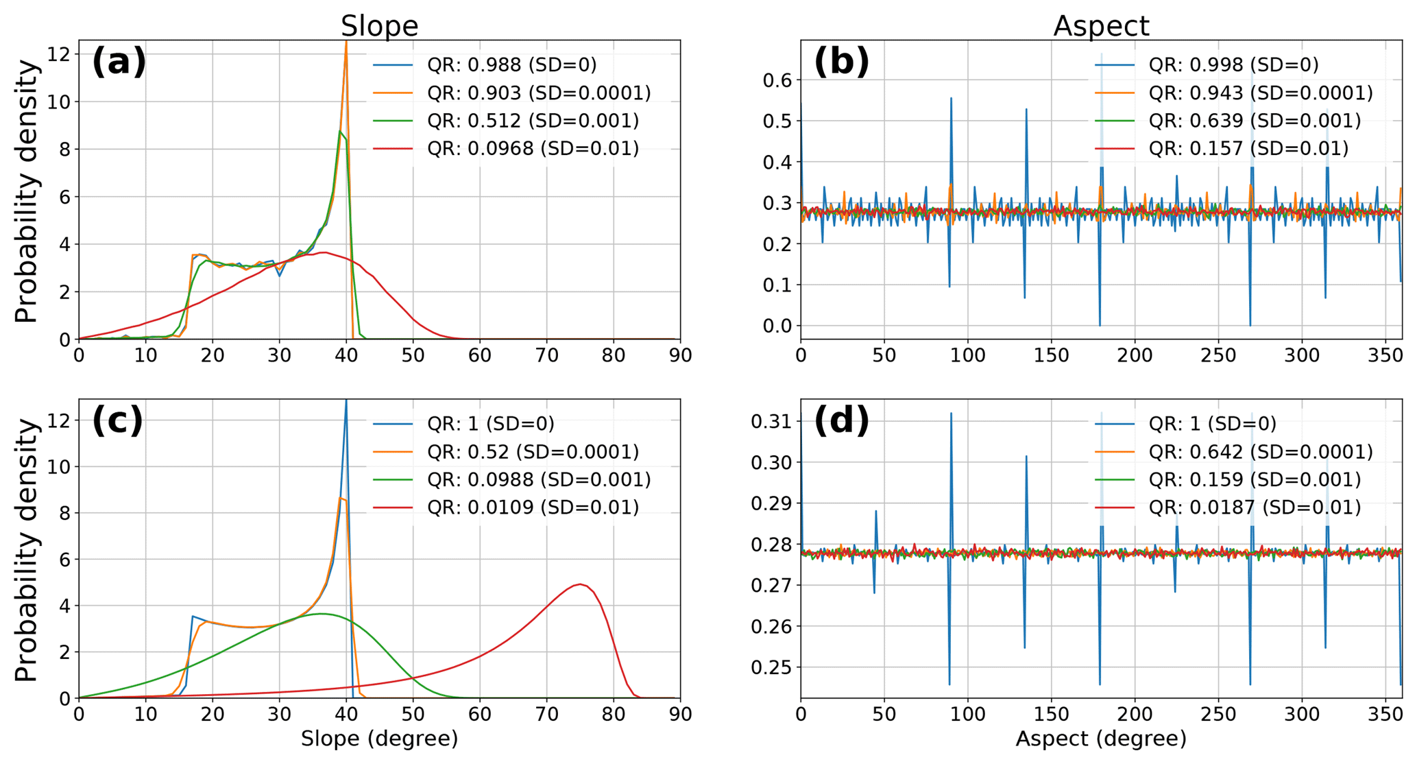
Figure 8Slope (a, c) and aspect (b, d) probability distributions (1∘ bins) for a Gaussian hill with homogeneous noise at variable levels (SD = 0, 1e−2, 1e−3, 1e−4) for n=101 (a, b) and n=1001 (c, d). The introduction of small levels of noise washes the spikes out of the aspect distribution. Slope distributions are steeper with the introduction of higher noise levels. Similar density functions are generated at similar QRs, despite differences in absolute noise levels.
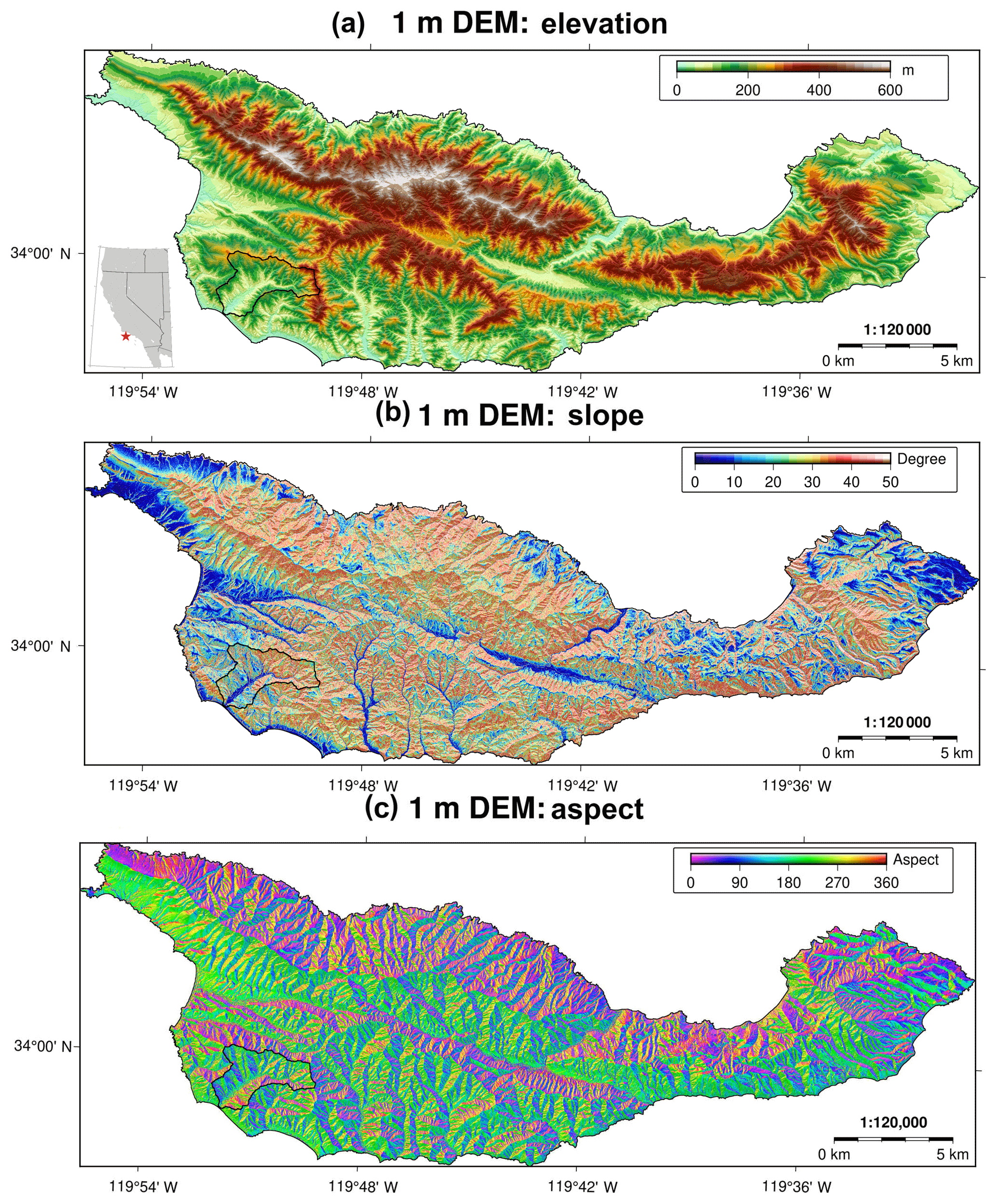
Figure 9Topographic setting of Santa Cruz Island (SCI), showing elevation (a), slope (b), and aspect (c) derived from a 1 m DEM and calculated from a total of 2.3×10⁹ ground-classified lidar points. The SCI covers a wide range of terrain types, slope regimes, and all aspect directions. The black polygon (southwest SCI) indicates the Pozo catchment shown in Fig. 10. For a canopy height model, we refer to Fig. S12.
6.2 Deriving elevations and uncertainties from point cloud data
Using LAStools (LAStools, 2017), we use a triangulated irregular network (TIN) approach to derive average point cloud elevations at each grid cell center, for each of our chosen grid resolutions (1–30 m, in 1 m steps, and 90 m). We have tested several alternative interpolation schemes – including simple means, inverse-distance weights, and other triangulation schemes – using all of the major open-source software packages (see Table S1 for a full listing and Figs. S13–S21 for a cross comparison). Each of these methods generates a slightly different DEM, with different assumptions and ideal use cases. Our optimal grid-resolution analysis is applicable to each of these DEMs; there is relatively little variation in grid-wide TE and PEU across interpolation schemes. To simplify our discussion of the lidar data, we use only the TIN DEM for further analysis. However, it is clear that our analyses of TE and PEU for slope and aspect are equally applicable to DEMs created with alternative interpolation schemes.
In addition to producing DEMs, we generate pixel-wise standard deviations estimated from the point cloud. That is, we determined the standard deviation of all ground-classified lidar points falling into each grid cell for each grid resolution. While vegetation cover may impact ground-classification results, our calculations are based on ground-classified points only. Because of the high point-cloud density, this standard deviation metric should reflect terrain variability and not vegetation cover. This measure serves as a DEM uncertainty and is highly spatially heterogeneous. Elevation and standard deviation maps for additional grid resolutions can be found in the Supplement (Figs. S22–S24). An island-wide canopy-height model can be found in Fig. S12.
6.3 Mapping uncertainty on SCI
Using our standard deviation grids, we can then calculate both TE and PEU on SCI (see Fig. S25). Using these two grids as inputs, we can also derive the QR across the entire SCI (Fig. 10). Note that maximal QRs are low when compared to the theoretical models shown in Figs. 6 and 8; this is due to both the much higher inherent noise in the real-world data and to the more complex terrain represented by the lidar data.

Figure 10Selected metrics for the Pozo catchment in the southwestern part of SCI, calculated on the optimal grid resolution for this catchment (3 m grid): (a) elevation, (b) lidar point density, (c) elevation standard deviation, and (d) slope quality ratio (see Eq. 14). The aspect quality ratio is shown in Fig. S26. A comparison of the elevation standard deviation and the lidar canopy height model is shown in Fig. S27.
6.4 Identification of optimal grid resolution
Using our pixel-wise standard deviations – and derived QRs – at each grid resolution, we can determine the island-wide optimal grid resolution for the calculation of topographic metrics which minimizes the combined influence of TE and PEU on our lidar dataset.
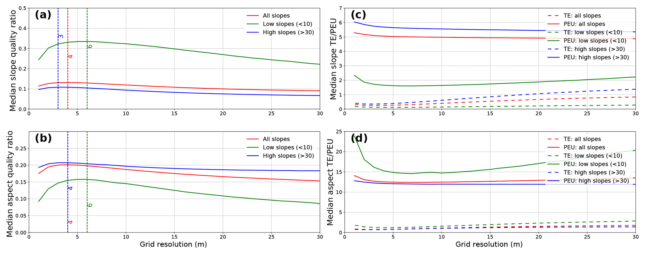
Figure 11Median QRs for all slopes, low slopes (<10), and high slopes (>30) across grid resolutions (1–30 m). There is a clear trend where low slopes have better slope QRs but worse aspect QRs. The optimal grid resolution for SCI is 4 m for both slope and aspect. For interquartile ranges on the QRs, see Fig. S28.
Unlike the synthetic data examined in Fig. 6, the optimal grid resolution for aspect calculations is the same as that for slope. This is due to the distribution of both elevations and elevation uncertainties in the SCI DEM and the different responses of slope and aspect calculations to the diverse terrain on SCI. Whole-island median TE, PEU, and QR can be found in Table S2 for grid resolutions from 1 to 10 m. While 4 m is the calculated optimal grid resolution, the QR peak is quite flat (see Fig. 11), implying that both 3 and 5 m DEMs will yield slope and aspect results of nearly equal quality. Indeed, the TE and PEU magnitudes are similar for both metrics between 3 and 5 m (see Table S2).
It should be noted that a 4 m optimal grid resolution is likely too large for many applications, particularly those interested in microtopography or other small-scale features. In those cases, slope and aspect values calculated from a higher-resolution DEM should be used with caution – PEU will continue to grow as grid resolution increases, and the rate of that increase will accelerate (see Fig. 5). This effect will occur even if the DEM uncertainty decreases at smaller scales simply due to the larger impacts of PEU at very high grid resolutions. This means that the uncertainty bounds on slope and aspect estimates on very high-resolution DEMs will increase quickly, which may limit some analyses. It is important to examine whether the data are precise enough to effectively resolve the features of interest. For high-resolution analyses, very high-quality DEMs are required.
In this analysis of the airborne lidar dataset from SCI, we find that a 4 m DEM resolution minimizes the combined influence of TE and PEU. Slope and aspect analyses performed at this grid resolution have the smallest error bounds and thus provide the most reliable data for analysis of topographic metrics over the entire island. However, there exist other methods of choosing an appropriate DEM resolution for a given analysis, for example, that of Roering et al. (2010). We do not argue that our method is the best for all applications but that our optimal grid resolution provides the smallest uncertainty for slope and aspect calculations over the entire dataset.
While a single, whole-island grid resolution is useful in some applications, it is clear from Fig. 10 that there are large spatial variations in the DEM uncertainty and the resulting QR, and hence in the optimal grid resolution. We can extend our method of identifying the optimal grid resolution on a catchment-by-catchment basis (Fig. 12, map view in Fig. S29).
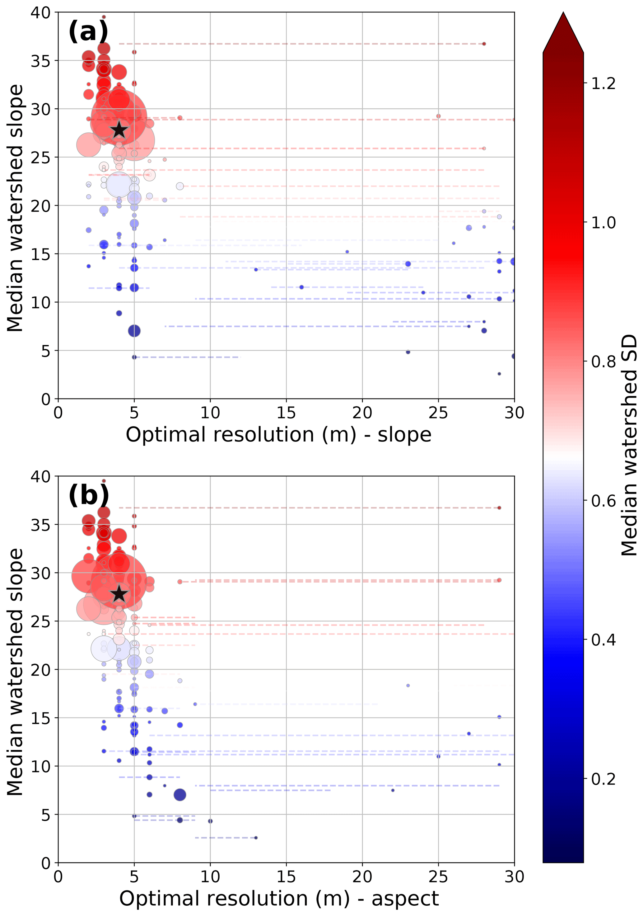
Figure 12Optimal grid resolution for minimizing error bounds on slope and aspect calculations across SCI compared to catchment median slope. Point sizes are scaled to catchment size, from 0.1 to 34 km2. Dashed lines show the 25th percentile to 75th percentile of optimal grid resolution, colored by the standard deviation of that point. Stars show the whole-island optimal resolution and median slope. There exists a clear trend where lower median slopes lead to lower optimal grid resolutions. Standard deviations also tend to be smaller in these catchments, due to higher DEM fidelity over flat terrain. Catchments with low (>10 m) optimal grid resolutions are small and have complex topography. For a map view of these results, we refer to Fig. S29.
There exist large spatial variations in the optimal grid resolution across SCI, driven by differences in terrain slope and DEM quality. When these differences are compared to median catchment slope and median catchment standard deviation, a clear pattern emerges (Fig. 12). While there remains significant scatter in the data, catchments with high median slopes tend to have both higher standard deviations and lower optimal grid resolutions. The data are bimodal, with the majority (83 % for slope, 95 % for aspect) of catchments having optimal resolutions below 10 m.
It is worth noting that the vast majority of the catchments with optimal slope and aspect resolutions above 10 m are small catchments concentrated on the northwestern edge of SCI (see Fig. S29). These catchments have two unique topographic features which contribute to the high optimal grid sizes. (1) They have two distinct slope regimes: one steep hill of nearly constant slope, followed by one flatter residual marine terrace with a different constant slope. (2) The catchments drain into steep, deeply incised cliffs. Interestingly, neither removing the steep cliffs (which have high elevation uncertainty) nor aggregating several small catchments into one larger analysis unit (to improve the statistical reliability of the median QR) results in higher optimal grid resolutions. We posit that the low optimal grid resolutions are a product of the unique two-stage topography in this region. However, an in-depth analysis of the specific factors which drive the optimal terrain resolution in each individual zone is outside of the scope of this paper.
As a final application, we clipped out only the river networks on SCI to test whether they had higher or lower optimal grid resolutions than the island as a whole or their individual catchments. We found that river networks, particularly those parts of the network which are in steep terrain, have higher elevation uncertainties, which leads to predicted higher optimal grid resolutions than the surrounding terrain. In applying our method of deriving optimal grid resolution, it is important to take into account the possibility of large differences in the optimal grid resolution over relatively small spatial scales and to account for the differences in elevation uncertainty in different terrain types.
6.5 Island-wide slope and aspect distributions
As has been shown in Figs. 6 and 11, there is clearly an optimal spatial resolution for the calculation of slope and aspect on our SCI lidar dataset. Furthermore, in Fig. 8, it was shown that changes in QR can have a substantial impact on the slope and aspect distributions of a synthetic surface. This analysis can be extended to the SCI lidar data at a range of spatial scales (Fig. 13).
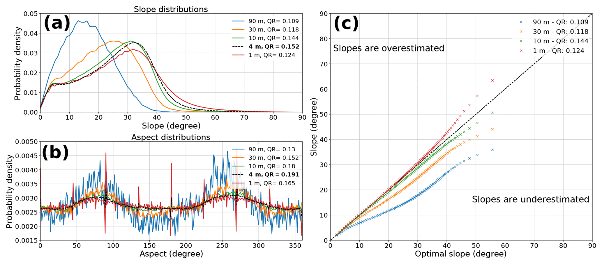
Figure 13(a) Slope and (b) aspect differences across SCI DEMs, with QR calculated using SCI DEM elevation standard deviations (see Figs. 10 and S22–S24). Optimal slope and aspect distributions are plotted in black. (c) Quantile–quantile plot showing difference between the entire SCI slope distribution vs. the “optimal” (4 m) resolution. We observe a clear pattern in slope distributions where resolutions below the optimal resolution tend to overestimate slope, and those below tend to underestimate slope.
There are clear differences in the slope and aspect distributions with increasingly poor QRs. This effect can also be seen in quantile–quantile plots of the entire SCI slope distribution when compared to the optimal grid resolution (see Fig. 13c). Grid resolutions higher than the optimal result in slope distributions that are dominated by higher slopes, while lower resolutions tend towards lower slopes. This effect can be seen even when the grid resolution is only slightly removed from the optimal resolution (Fig. S30). Notably, grid resolutions close to the optimal (e.g., 3 and 5 m) have QRs and slope distributions that are very similar to the optimal 4 m distribution.

Figure 14(a) Divergence of higher and lower grid-resolution slope distributions from that at the optimal resolution for the Pozo catchment (see Fig. 9). Except for the 1 m histogram, the differences between resolutions are small. Right panels show slope distributions taken from 1, 2, 4, and 5 m data resampled to 3 m resolution using (b) bilinear resampling and (c) nearest-neighbor resampling. The resampled data distributions do not converge on the reference 3 m distribution, except for the 1 m data resampled with a nearest-neighbor approach.
As a final test of grid-resolution dependence, we resampled several grids to nominally match the optimal grid resolution – in this case, we chose 3 m for the Pozo catchment (see Figs. 9, S31) as the reference distribution. As can be seen in Fig. 14a, there are differences between test (1–5 m) resolutions and the reference 3 m histogram. When the test datasets are resampled to the 3 m reference resolution using bilinear resampling (Fig. 14b) and nearest-neighbor resampling (Fig. 14c), the histograms generally do not converge to the reference 3 m distribution. The exception to this is when the 1 m data are resampled with a nearest-neighbor approach, they converge to the 3 m distribution. We attribute this effect to the lidar-gridding method – the 3 m data are drawn from the same neighborhood as the nine 1 m neighborhoods which are used for the 1 m gridding.
In general, slope distributions from resampled data should be used with caution; simply resampling elevation data to the optimal grid resolution before calculating slope does not guarantee better results – the DEM has to be created from the ungridded point data to fully take advantage of optimal gridding for slope calculations.
This study presents a detailed account of uncertainties and errors in the calculation of terrain slope and aspect derived from both truncation errors and uncertainty in the underlying source DEM. We first develop our analysis on synthetic data, which act as a control dataset. We then extend our methodology onto a high point-density lidar dataset, which allows us to compare the relative impacts of gridding truncation errors and propagated elevation uncertainty on the calculation of topographic metrics.
From the analysis of both synthetic and real-world data, we identify the following key points: (1) the relative impact of truncation error and propagated elevation uncertainty can be captured in a single metric, which we call the quality ratio. This metric can be used to compare the accuracy of topographic metrics across DEM spatial resolutions and uncertainty distributions. (2) There exists an optimal grid resolution at which to calculate terrain slope and aspect for a given dataset that minimizes the total impact of both truncation error and propagated elevation uncertainty; the distribution of DEM uncertainties leads to spatial variation in the optimal grid resolutions at which to calculate slope and aspect. For Santa Cruz Island in southern California, we find an optimal grid resolution of 4 m, with island-average slope (aspect) errors of 0.25∘ (0.75∘) for truncation error and 5∘ (12.5∘) for propagated elevation uncertainty. (3) Topographic metrics calculated at suboptimal grid resolutions will have potentially large errors in their slope and aspect distributions. Resampling grids to the optimal resolution does not completely ameliorate these issues; it is important to generate the DEM at the optimal resolution from the underlying lidar dataset. (4) Slope and aspect calculations at high DEM resolutions (<3 m) are significantly impacted by the nonlinear relationship between grid spacing and propagated elevation uncertainty. A DEM with very low uncertainties is required to support robust analysis of fine-scale topography.
Given that grid-resolution-driven effects on regional slope and aspect distributions could have significant impacts on the interpretation of landscape morphology, we recommend that region-specific optimal DEM resolutions be determined before the calculation of topographic metrics.
All codes and data for reproducing the results can be found in Smith et al. (2019). Updates to the software can be found on GitHub at https://github.com/UP-RS-ESP/TopoMetricUncertainty (last access: 17 May 2019).
The supplement related to this article is available online at: https://doi.org/10.5194/esurf-7-475-2019-supplement.
TS led the development and writing of the MS, as well as the primary data analysis. AR contributed to the development of the methods and developed most of the Python codes. BB contributed to the development of the methods and processed the lidar data.
The authors declare that they have no conflict of interest.
The authors thank Fiona Clubb and Ben Purinton for comments on an earlier version of the manuscript.
This research has been supported by the State of Brandenburg (Germany) through the Ministry of Science and Education, the NEXUS project, the Deutsche Forschungsgemeinschaft (German Research Foundation) and Open Access Publication Fund of Potsdam University.
This paper was edited by Giulia Sofia and reviewed by Marco Cavalli and two anonymous referees.
Abarbanel, S., Ditkowski, A., and Gustafsson, B.: On error bounds of finite difference approximations to partial differential equations–temporal behavior and rate of convergence, J. Sci. Comput., 15, 79–116, 2000. a, b
Ayalew, L. and Yamagishi, H.: The application of GIS-based logistic regression for landslide susceptibility mapping in the Kakuda-Yahiko Mountains, Central Japan, Geomorphology, 65, 15–31, 2005. a
Baguskas, S. A., Peterson, S. H., Bookhagen, B., and Still, C. J.: Evaluating spatial patterns of drought-induced tree mortality in a coastal California pine forest, Forest Ecol. Manag., 315, 43–53, 2014. a
Band, L. E.: Topographic partition of watersheds with digital elevation models, Water Resour. Res., 22, 15–24, 1986. a
Bolstad, P. V. and Stowe, T.: An evaluation of DEM accuracy: elevation, slope, and aspect, Photogramm. Eng. Rem. S., 60, 7327–7332, 1994. a
Bookhagen, B. and Strecker, M. R.: Spatiotemporal trends in erosion rates across a pronounced rainfall gradient: Examples from the southern Central Andes, Earth Planet. Sc. Lett., 327, 97–110, 2012. a, b
Carlisle, B. H.: Modelling the spatial distribution of DEM error, T. GIS, 9, 521–540, 2005. a
Dibblee, T. W.: Geologic Map of Western Santa Cruz Island, Dibblee Geological Foundation, Santa Barbara, California, USA, 2001. a
Dietrich, W. E., Bellugi, D. G., Sklar, L. S., Stock, J. D., Heimsath, A. M., and Roering, J. J.: Geomorphic transport laws for predicting landscape form and dynamics, Prediction in geomorphology, 135, 103–132, 2003. a
Dunn, M. and Hickey, R.: The effect of slope algorithms on slope estimates within a GIS, Cartography, 27, 9–15, 1998. a, b
Durran, D. R.: Numerical methods for wave equations in geophysical fluid dynamics, vol. 32, Springer Science & Business Media, New York, USA, 1999. a
Evans, I. S.: An integrated system of terrain analysis and slope mapping, Z. Geomorphol., 36, 274–295, 1980. a, b, c, d
Farr, T. G., Rosen, P. A., Caro, E., Crippen, R., Duren, R., Hensley, S., Kobrick, M., Paller, M., Rodriguez, E., Roth, L., Seal, D., Shaffer, S., Shimada, J., Umland, J., Werner, M., Oskin, M., Burbank, D., and Alsdorf, D.: The shuttle radar topography mission, Rev. Geophys., 45, RG2004, https://doi.org/10.1029/2005RG000183, 2007. a
Fisher, P. F.: Models of uncertainty in spatial data, Geographical information systems, 1, 191–205, 1999. a
Fisher, P. F. and Tate, N. J.: Causes and consequences of error in digital elevation models, Prog. Phys. Geog., 30, 467–489, 2006. a
Florinsky, I. V.: Accuracy of local topographic variables derived from digital elevation models, Int. J. Geogr. Inf. Sci., 12, 47–62, 1998. a, b, c, d
Fornberg, B.: Generation of finite difference formulas on arbitrarily spaced grids, Math. Comput., 51, 699–706, 1988. a
Franklin, J.: Predictive vegetation mapping: geographic modelling of biospatial patterns in relation to environmental gradients, Prog. Phys. Geog., 19, 474–499, 1995. a
Grieve, S. W. D., Mudd, S. M., Milodowski, D. T., Clubb, F. J., and Furbish, D. J.: How does grid-resolution modulate the topographic expression of geomorphic processes?, Earth Surf. Dynam., 4, 627–653, https://doi.org/10.5194/esurf-4-627-2016, 2016. a
Guisan, A. and Zimmermann, N. E.: Predictive habitat distribution models in ecology, Ecol. Model., 135, 147–186, 2000. a
Guzzetti, F., Carrara, A., Cardinali, M., and Reichenbach, P.: Landslide hazard evaluation: a review of current techniques and their application in a multi-scale study, Central Italy, Geomorphology, 31, 181–216, 1999. a
Heuvelink, G. B., Burrough, P. A., and Stein, A.: Propagation of errors in spatial modelling with GIS, Int. J. Geog. Inf. Syst., 3, 303–322, 1989. a, b, c
Holmes, K., Chadwick, O., and Kyriakidis, P. C.: Error in a USGS 30-meter digital elevation model and its impact on terrain modeling, J. Hydrol., 233, 154–173, 2000. a
Hunter, G. J. and Goodchild, M. F.: Modeling the uncertainty of slope and aspect estimates derived from spatial databases, Geogr. Anal., 29, 35–49, 1997. a, b, c
Kent, M.: Vegetation description and data analysis: a practical approach, John Wiley & Sons, New York, USA, 2011. a
Kirby, E. and Whipple, K. X.: Expression of active tectonics in erosional landscapes, J. Struct. Geol., 44, 54–75, 2012. a
Kraus, K. and Pfeifer, N.: Determination of terrain models in wooded areas with airborne laser scanner data, ISPRS J. Photogramm., 53, 193–203, 1998. a
Kyriakidis, P. C., Shortridge, A. M., and Goodchild, M. F.: Geostatistics for conflation and accuracy assessment of digital elevation models, Int. J. Geog. Inf. Sci., 13, 677–707, 1999. a
Lague, D.: The stream power river incision model: evidence, theory and beyond, Earth Surf. Proc. Land., 39, 38–61, 2014. a
LAStools: Efficient LiDAR Processing Software (version 180831, academic), available at: http://rapidlasso.com/LAStools (last access: 12 January 2019), 2017. a
Lee, J., Fisher, P., Snyder, P., et al.: Modeling the effect of data errors on feature extraction from digital elevation models, Photogramm. Eng. Rem. S., 58, 1461–1461, 1992. a
Montgomery, D. R. and Dietrich, W. E.: A physically based model for the topographic control on shallow landsliding, Water Resour. Res., 30, 1153–1171, 1994. a
Mukul, M., Srivastava, V., Jade, S., and Mukul, M.: Uncertainties in the Shuttle Radar Topography Mission (SRTM) Heights: Insights from the Indian Himalaya and Peninsula, Sci. Rep., 7, 41672, https://doi.org/10.1038/srep41672, 2017. a
Neely, A., Bookhagen, B., and Burbank, D.: An automated knickzone selection algorithm (KZ-Picker) to analyze transient landscapes: Calibration and validation, J. Geophys. Res.-Earth, 122, 1236–1261, 2017. a
Oksanen, J. and Sarjakoski, T.: Error propagation of DEM-based surface derivatives, Comput. Geosci., 31, 1015–1027, 2005. a, b, c
Oksanen, J. and Sarjakoski, T.: Uncovering the statistical and spatial characteristics of fine toposcale DEM error, Int. J. Geog. Inf. Sci., 20, 345–369, 2006. a
OpenTopography: 2010 channel islands lidar collection, https://doi.org/10.5069/G95D8PS7, 2012. a
Ouma, Y. O. and Tateishi, R.: Urban flood vulnerability and risk mapping using integrated multi-parametric AHP and GIS: methodological overview and case study assessment, Water, 6, 1515–1545, 2014. a
Pelletier, J. D.: Quantitative modeling of earth surface processes, Cambridge University Press, Cambridge, UK, https://doi.org/10.1017/CBO9780511813849, 2008. a
Pelletier, J. D.: Minimizing the grid-resolution dependence of flow-routing algorithms for geomorphic applications, Geomorphology, 122, 91–98, 2010. a
Pelletier, J. D.: A robust, two-parameter method for the extraction of drainage networks from high-resolution digital elevation models (DEMs): Evaluation using synthetic and real-world DEMs, Water Resour. Res., 49, 75–89, 2013. a
Perroy, R. L., Bookhagen, B., Asner, G. P., and Chadwick, O. A.: Comparison of gully erosion estimates using airborne and ground-based LiDAR on Santa Cruz Island, California, Geomorphology, 118, 288–300, 2010. a
Perroy, R. L., Bookhagen, B., Chadwick, O. A., and Howarth, J. T.: Holocene and Anthropocene landscape change: arroyo formation on Santa Cruz Island, California, Ann. Assoc. Am. Geogr., 102, 1229–1250, 2012. a
Pierce, K. B., Lookingbill, T., and Urban, D.: A simple method for estimating potential relative radiation (PRR) for landscape-scale vegetation analysis, Landscape Ecol., 20, 137–147, 2005. a
Purinton, B. and Bookhagen, B.: Validation of digital elevation models (DEMs) and comparison of geomorphic metrics on the southern Central Andean Plateau, Earth Surf. Dynam., 5, 211–237, https://doi.org/10.5194/esurf-5-211-2017, 2017. a, b
Purinton, B. and Bookhagen, B.: Measuring decadal vertical land-level changes from SRTM-C (2000) and TanDEM-X (∼2015) in the south-central Andes, Earth Surf. Dynam., 6, 971–987, https://doi.org/10.5194/esurf-6-971-2018, 2018. a, b
Rodriguez, E., Morris, C. S., and Belz, J. E.: A global assessment of the SRTM performance, Photogramm. Eng. Rem. S., 72, 249–260, 2006. a
Roering, J. J., Kirchner, J. W., and Dietrich, W. E.: Evidence for nonlinear, diffusive sediment transport on hillslopes and implications for landscape morphology, Water Resour. Res., 35, 853–870, 1999. a
Roering, J. J., Marshall, J., Booth, A. M., Mort, M., and Jin, Q.: Evidence for biotic controls on topography and soil production, Earth Planet. Sc. Lett., 298, 183–190, 2010. a
Schmidt, J., Evans, I. S., and Brinkmann, J.: Comparison of polynomial models for land surface curvature calculation, Int. J. Geog. Inf. Sci., 17, 797–814, 2003. a, b
Shortridge, A. and Messina, J.: Spatial structure and landscape associations of SRTM error, Remote Sens. Environ., 115, 1576–1587, 2011. a
Skidmore, A. K.: A comparison of techniques for calculating gradient and aspect from a gridded digital elevation model, Int. J. Geog. Inf. Syst., 3, 323–334, 1989. a, b
Smith, B. and Sandwell, D.: Accuracy and resolution of shuttle radar topography mission data, Geophys. Res. Lett., 30, 1467, https://doi.org/10.1029/2002GL016643, 2003. a, b
Smith, T., Rheinwalt, A., and Bookhagen, B.: TopoMetricUncertainty – Calculating Topographic Metric Uncertainty and Optimal Grid Resolution. V. 1.0, GFZ Data Services, https://doi.org/10.5880/fidgeo.2019.017, 2019. a
Snyder, N. P., Whipple, K. X., Tucker, G. E., and Merritts, D. J.: Landscape response to tectonic forcing: Digital elevation model analysis of stream profiles in the Mendocino triple junction region, northern California, Geol. Soc. Am. Bull., 112, 1250–1263, 2000. a
Tarboton, D. G.: A new method for the determination of flow directions and upslope areas in grid digital elevation models, Water Resour. Res., 33, 309–319, 1997. a, b, c, d, e
Thompson, J. A., Bell, J. C., and Butler, C. A.: Digital elevation model resolution: effects on terrain attribute calculation and quantitative soil-landscape modeling, Geoderma, 100, 67–89, 2001. a
Tucker, G. E. and Bras, R. L.: Hillslope processes, drainage density, and landscape morphology, Water Resour. Res., 34, 2751–2764, 1998. a
Tucker, G. E. and Hancock, G. R.: Modelling landscape evolution, Earth Surf. Proc. Land., 35, 28–50, 2010. a
Wechsler, S. P.: Uncertainties associated with digital elevation models for hydrologic applications: a review, Hydrol. Earth Syst. Sci., 11, 1481–1500, https://doi.org/10.5194/hess-11-1481-2007, 2007. a, b
Wechsler, S. P. and Kroll, C. N.: Quantifying DEM uncertainty and its effect on topographic parameters, Photogramm. Eng. Rem. S., 72, 1081–1090, 2006. a, b
Wessel, B., Huber, M., Wohlfart, C., Marschalk, U., Kosmann, D., and Roth, A.: Accuracy assessment of the global TanDEM-X Digital Elevation Model with GPS data, ISPRS J. Photogramm., 139, 171–182, 2018. a
Whipple, K. X. and Tucker, G. E.: Dynamics of the stream-power river incision model: Implications for height limits of mountain ranges, landscape response timescales, and research needs, J. Geophys. Res.-Sol. Ea., 104, 17661–17674, 1999. a
Zevenbergen, L. W. and Thorne, C. R.: Quantitative analysis of land surface topography, Earth Surf. Proc. Land., 12, 47–56, 1987. a, b, c
Zhang, J. and Goodchild, M. F.: Uncertainty in geographical information, CRC press, London, UK, https://doi.org/10.1201/b12624, 2002. a
Zhang, W. and Montgomery, D. R.: Digital elevation model grid size, landscape representation, and hydrologic simulations, Water Resour. Res., 30, 1019–1028, 1994. a
Zhou, Q. and Liu, X.: Error analysis on grid-based slope and aspect algorithms, Photogramm. Eng. Rem. S., 70, 957–962, 2004. a, b, c, d, e
- Abstract
- Introduction
- Data and methods
- Sources of uncertainty in topographic metrics
- Optimal grid spacing
- Impacts of noise on topographic distributions
- Case study: multi-resolution lidar on Santa Cruz Island
- Conclusions
- Code and data availability
- Author contributions
- Competing interests
- Acknowledgements
- Financial support
- Review statement
- References
- Supplement