A photogrammetry-based approach for soil bulk density measurements with an emphasis on applications to cosmogenic nuclide analysis

The quantification of soil bulk density (ρ_B) is a cumbersome and time-consuming task when traditional soil density sampling techniques are applied. However, it can be important for terrestrial cosmogenic nuclide (TCN) production rate scaling when deriving ages or surface process rates from buried samples, in particular when short-lived TCNs such as in situ ¹⁴C are applied. Here, we show that soil density determinations can be made using structure-from-motion multi-view stereo (SfM-MVS) photogrammetry-based volume reconstructions of sampling pits. Accuracy and precision tests as found in the literature and as conducted in this study clearly indicate that photographs taken from both a consumer-grade digital single-lens mirrorless (DSLM) and a smartphone camera are of sufficient quality to produce accurate and precise modelling results, i.e. to regularly reproduce the “true” volume and/or density by >95 %. This finding holds also if a freeware-based computing workflow is applied. The technique has been used to measure ρ_B along three small-scale (<1 km) N–S transects located in the semi-arid to arid Altos de Talinay, northern central Chile (∼30.5^∘ S, ∼71.7^∘ W), during a TCN sampling campaign. Here, long-term differences in microclimatic conditions between south-facing and north-facing slopes (SFSs and NFSs, respectively) explain a sharp contrast in vegetation cover, slope gradient and general soil condition patterns. These contrasts are also reflected by the soil density data, generally coinciding with lower densities on SFSs. The largest differences between NFSs and SFSs are evident in the lower portion of the respective slopes, close to the thalwegs. In general, field-state soil bulk densities were found to vary by about 0.6 g cm⁻³ over a few tens of metres along the same slope. As such, the dataset that was mainly generated to derive more accurate TCN-based process rates and ages can be used to characterise the present-day condition of soils in the study area, which in turn can give insight into the long-term soil formation and prevailing environmental conditions. This implies that the method tested in this study may also being applied in other fields of research and work, such as soil science, agriculture or the construction sector.

1 Introduction

Soil density determination is a time-consuming task when sampling for a terrestrial cosmogenic nuclide (TCN)-based analysis, but it is an important parameter if process rates and/or ages are inferred from the final nuclide concentration (e.g. Rodés and Evans, 2020; Rodés et al., 2011). This is because the spallogenic production rates of TCNs are typically assumed to decrease exponentially with increasing depth z below the surface at a rate which is partially dependent on the subsurface density (e.g. Dunai, 2010; Lal, 1991; Lal and Arnold, 1985; Nishiizumi et al., 1986):

$$\begin{array}{}\text{(1)}& P\left(z\right)=P_{\mathrm{0}}{e}^{-\mathit{\rho }z/\mathrm{\Lambda }},\end{array}$$

where P₀ is the production at the Earth's surface and Λ denotes the attenuation length (Eq. 1 valid for non-eroding surfaces). The density ρ denotes the density of the material through which the cosmic rays traverse below the surface, i.e. the density of soil, saprolite and/or rock (e.g. Heimsath and Jungers, 2013; Lal, 1991). The field-state bulk density (ρ_B,f) of a given excavated soil material is defined as

$$\begin{array}{}\text{(2)}& {\mathit{\rho }}_{\mathrm{B},\mathrm{f}}=m_{\mathrm{e},\mathrm{f}}{V}^{-\mathrm{1}},\end{array}$$

with m_e,f being the (field-state) mass of the excavated material and V the volume of the pit. Field-state and the corresponding dry bulk densities of soils (ρ_B,d) may vary over the larger-scale (e.g. basin-wide) erosion analysis, and thus the presumption of an averaged value for soil densities might be required in these cases. However, accurate knowledge about the value of ρ_B,f and/or ρ_B,d is more important for localised surface process rates or age inferences. The present-day soil (a term considered equivalent to regolith in this work; e.g. Heimsath et al., 1997) conditions represent only a glimpse of soil formation history, as environmental conditions, and thus the physical conditions of the subsurface, might have changed over the timescales that the cosmogenic-nuclide-derived process rates integrate over (e.g. Rodés et al., 2011). Nevertheless, they represent reasonable approximations, especially in scenarios of long-term steady-state erosion, i.e. where bedrock erosion equals soil production rates (e.g. Heimsath and Jungers, 2013; Heimsath et al., 1997). The imperative to obtain accurate knowledge of present-day soil densities increases if short-lived TCNs, such as in situ ¹⁴C, are analysed. In such a case, soil conditions are more likely to have prevailed over the time span during which the nuclide concentration has built up. Average densities of ordinary soils range between >1.0 and 1.8 g cm⁻³ (Hartel, 2005; Manrique and Jones, 1991; Schaetzl and Thompson, 2015) but can be greater or lower than this range, for example depending on their organic content, water content and/or degree of compaction (Schaetzl and Thompson, 2015). With respect to ¹⁰Be production in a soil column, nuclide production (including spallogenic and muogenic production) increases by about 49 % at a depth of 100 cm below the surface in a soil with ρ=1.1 g cm⁻³ when compared to a soil with ρ=1.8 g cm⁻³ (in situ ¹⁴C: ∼32 %; Fig. 1). Comparing the low-density soil to a highly compacted soil, for example with ρ=2.3 g cm⁻³ (Schaetzl and Thompson, 2015), would yield a doubling (97 % increase) of the ¹⁰Be production at 100 cm depth (in situ ¹⁴C: ∼58 %). These numbers exceed the analytical uncertainties, which are <10 % in most cases for measurements of medium to high ¹⁰Be and in situ ¹⁴C concentrations (e.g. Balco, 2017; Hippe, 2017). Thus, accurate knowledge of local regolith densities is important for in situ TCN-based process rate determinations, underlining the need for a reliable, adaptable and easy-to-apply method to determine excavation densities.

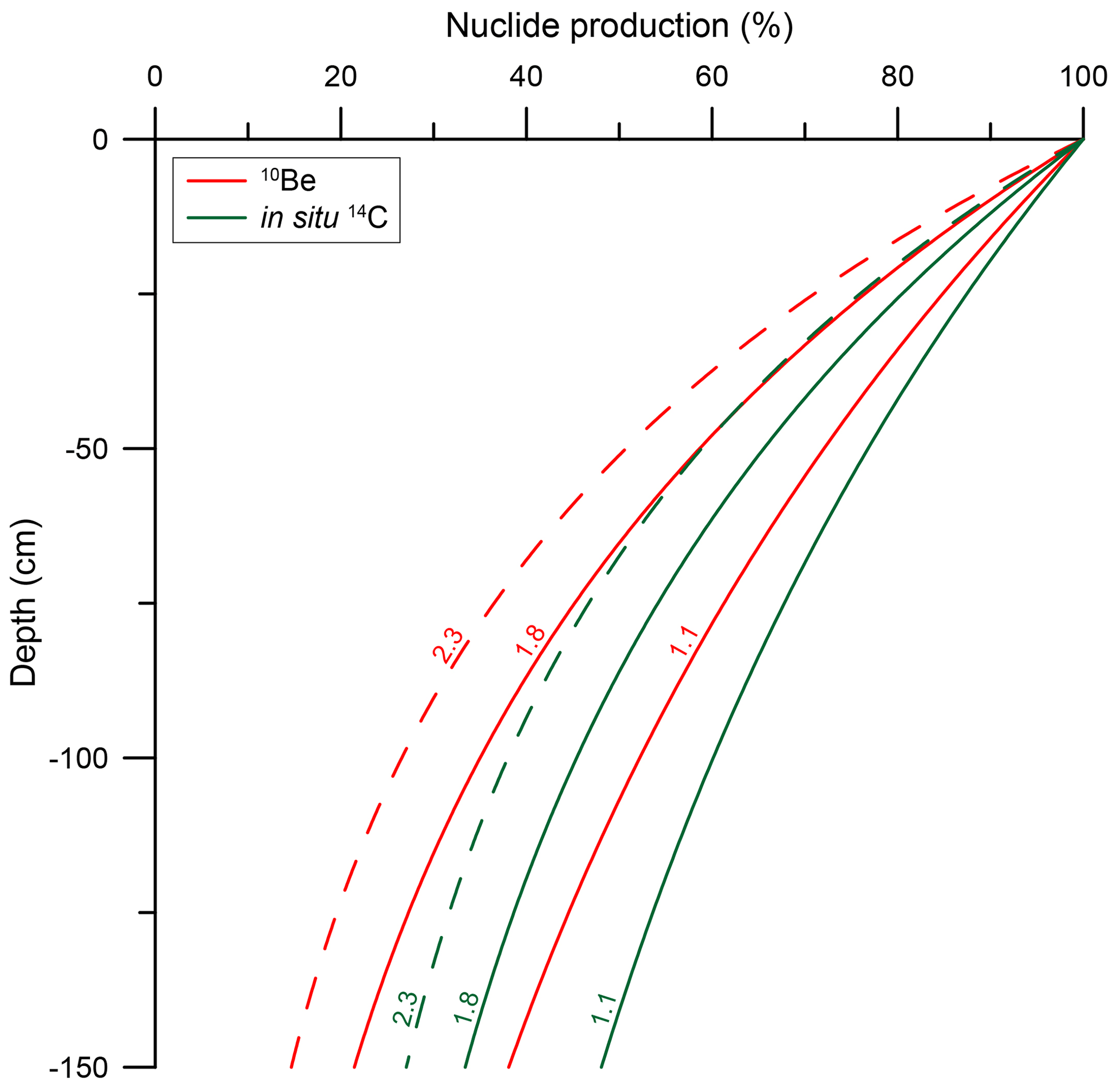
Figure 1 Depth and density dependence of nuclide production (non-eroding surfaces) within homogenous material. Solid lines represent two endmember densities (1.1 and 1.8 g cm⁻³; e.g. Hartel, 2005; Manrique and Jones, 1991; Schaetzl and Thompson, 2015) of typical soils (red: ¹⁰Be; green: in situ ¹⁴C). Dashed lines reflect nuclide production for highly compacted soils (2.3 g cm⁻³; Schaetzl and Thompson, 2015). Calculated for SLHL using the LSDn (Sa) scaling scheme (Lifton et al., 2014) with a spallogenic production rate of 3.92±0.31 at g⁻¹ yr⁻¹ for ¹⁰Be and 12.76±0.00 at g⁻¹ yr⁻¹ for ¹⁴C (Borchers et al., 2016; Phillips et al., 2016) and including the contribution of muogenic production as implemented in the MATLAB code provided by Balco (2017).

The application of photogrammetric methods to infer soil bulk densities is a relatively recent field of research and has been successfully tested by Bauer et al. (2014) and Berney et al. (2018). Both studies found good agreements between soil densities/excavation volumes derived from traditional methods and those obtained using photogrammetry (basic concepts of photogrammetry, structure-from-motion multi-view stereo (SfM-MVS) photogrammetry and their general application in combination with non-invasive methods in geosciences are explained e.g. in Eltner et al., 2016; James and Robson, 2012; Westoby et al., 2012). Other commonly used techniques include the core method, the clod method, the nuclear radiation method, the automated three-dimensional laser scanning method, X-ray-based methods, the thermo-time domain reflectometry (TDR) method, and non-photogrammetry excavation methods or pedotransfer functions (PTFs; for comprehensive overviews and detailed descriptions see e.g. Al-Shammary et al., 2018; Blake and Hartge, 1986; Grossman and Reinsch, 2002; Hao et al., 2008; Page-Dumroese et al., 1999; Soil Survey Staff, 2014). These approaches usually have one or more of the following disadvantages: (1) the application is time-consuming; (2) expert knowledge on the tools or programming is required; (3) large amounts of sampling tools or samples need to be carried in the field; (4) the samples and/or the tools require a significant amount of carrying space; (5) the techniques are cost-intensive; (6) the techniques are hazardous to the applicant and/or the environment; (7) the results strongly depend on soil textures and porosity; (8) the precision of the measurements is low; and/or (9) a prior calibration is needed.

By contrast, the photogrammetry-based excavation method mostly seems to overcome the above-mentioned disadvantages (Bauer et al., 2014; Berney et al., 2018). This approach can be applied to any kind of regolith whose cohesion allows the excavation of soil pits that maintain their sidewalls without collapsing (e.g. Brye et al., 2004; Maynard and Curran, 2008; Muller and Hamilton, 1992). Furthermore, it can be used in remote locations and rough terrain and does not require a significant additional amount of material to be taken into the field. These characteristics make this technique well suited for researchers working in remote areas (in terms of distance to a storage place for samples and equipment) and whose capability for carrying sampling material is mainly based on manpower and backpack space. Such a scenario regularly applies to our TCN sampling teams of the University of Cologne (UoC), Germany, which was the reason why we tested a photogrammetric method comprehensively.

We focused on SfM-MVS photogrammetry because it is simple for non-experts to use, as most reconstruction steps are fully automated (Eltner et al., 2016). Further testing of photogrammetric methods to derive soil bulk densities from imagery acquired during fieldwork was also required, as Berney et al. (2018) only excavated very small volumes (∼1.1 L) from flat surfaces and Bauer et al. (2014) only simulated ideal laboratory and field sampling conditions (no direct sunlight). Lighting conditions, however, have been shown to significantly affect the quality and accuracy of SfM-MVS photogrammetry-derived models (Mosbrucker et al., 2017, and references therein). Thus, in order to assess if the technique is applicable under fieldwork conditions during a TCN sampling campaign, we tested its accuracy and precision by simulating different lighting scenarios, parent materials and pit orientations (i.e. dipping surfaces and vertical faces). As our intention is to contribute a method that can be adopted by the TCN community, our workflow either included the combined use of commercial and non-commercial software or was solely based on non-commercial software (under the premise that Microsoft's Windows 10 is used as the operating system). We further assumed end users of this approach would not be experts in photography, the SfM-MVS photogrammetry technique or programming. Previous studies (e.g. Micheletti et al., 2015; Thoeni et al., 2014) have shown that the image quality of smartphone cameras can be sufficient to generate high-precision models of topographic features. Thus, our tests included both a consumer-grade digital single-lens mirrorless (DSLM) camera and a smartphone camera, to assess the robustness of the method and whether smartphone cameras can be used as substitutes for higher-grade models with regards to the accuracy and precision of ρ_B,f determinations. Finally, we applied the method during a TCN sampling campaign in the Coastal Cordillera of northern central Chile, where we investigate the impact of aspect-related differences in microclimate and vegetation on Earth-shaping processes and the formation of topography along narrow transects (cf. Bernhard et al., 2018; Gutiérrez-Jurado and Vivoni, 2013a, b; Oeser et al., 2018). Therefore, soil densities were derived, initially to scale soil production rates inferred from saprolite TCN concentrations (e.g. Heimsath and Burke, 2013) across contrasting slope aspects. However, due to the simple and time-efficient application of the method, we extended our dataset of regolith densities along the respective slopes in order to study aspect-related differences in this particular soil property.

2 Methods

2.1 Imaging testing scenarios, part 1: simulating a soil pit

To evaluate the accuracy and precision of the SfM-MVS photogrammetry-based excavation method and to test convenient workflows to obtain values for ρ_B,f and ρ_B,d, we adopted a two-phase testing procedure (Fig. 2). The first phase consisted of the simulation of a soil pit. For this we used the interior of a square flowerpot, on top of which a board was attached, imitating a soil surface. Into the board we cut a square hole that would fit the opening of the flowerpot (Fig. 3 and Supplement). The hole could be covered by a thin fabric cover to simulate the pre-dug surface; removing the fabric cover would simulate the pit after digging, measuring 22 cm × 22 cm × 23 cm (width × length × depth; Table 1). The cubic shape of the flowerpot differs from that of a semi-circular pit, which has been found to be the optimal shape to reconstruct the surface of the pit using SfM photogrammetry (Berney et al., 2018).

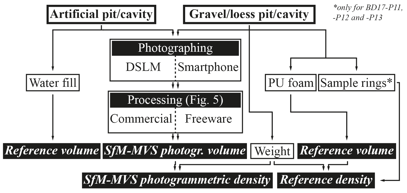
Figure 2 Generalised workflow applied to obtain SfM-MVS photogrammetry-based volumes, reference volumes and field-state soil bulk densities for testing purposes.

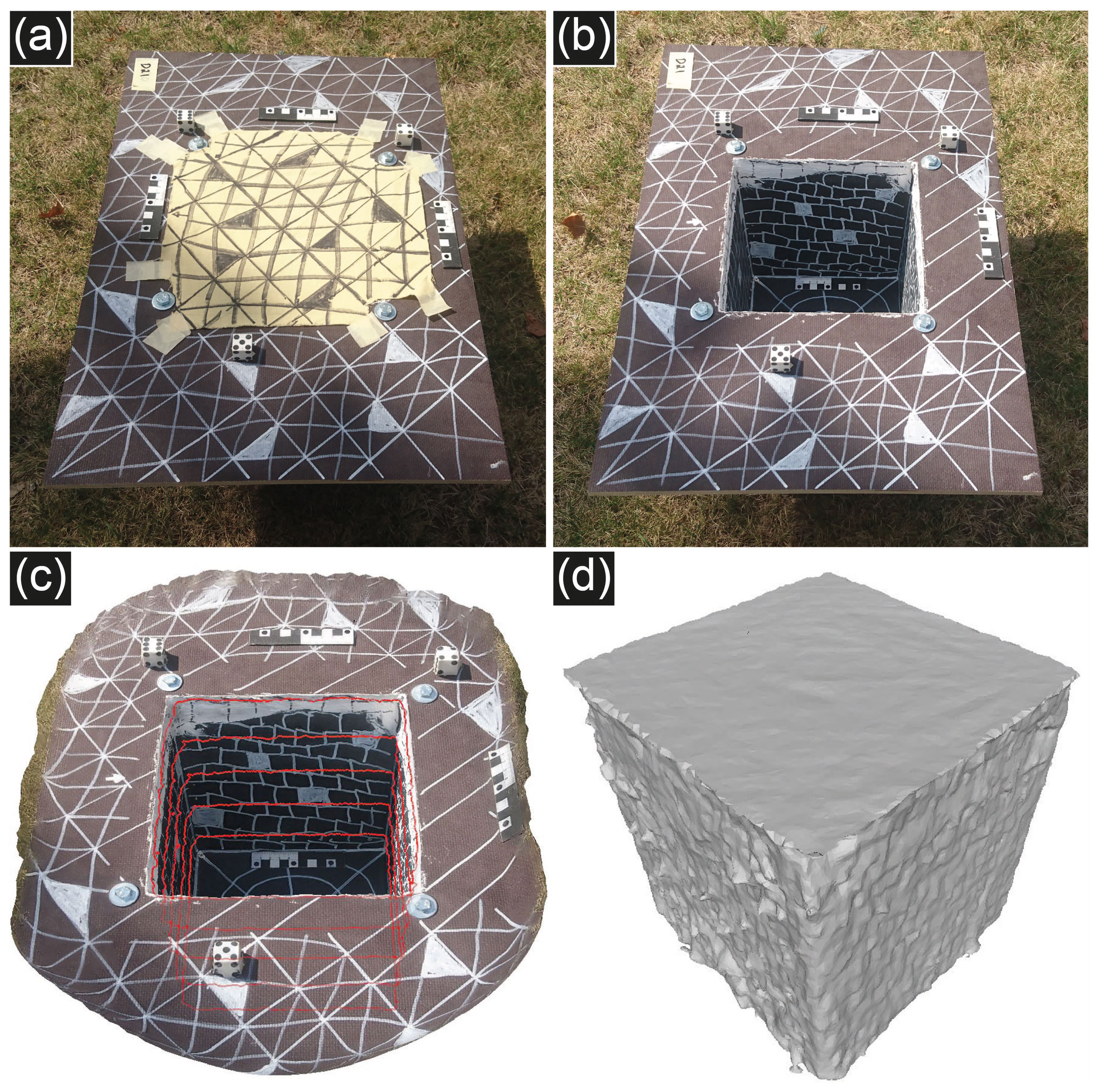
Figure 3 The flowerpot with a board attached (D21) with (a) and without (b) the thin fabric covering the opening. The reconstructed artificial pit is shown with 5 cm contours in red (c). To obtain the final watertight mesh, the reconstructions of simulated pre-dug surface and soil pit were merged by bridging the edges of the two meshes (d).

Table 1 Test pit designs used for the imaging testing scenarios.

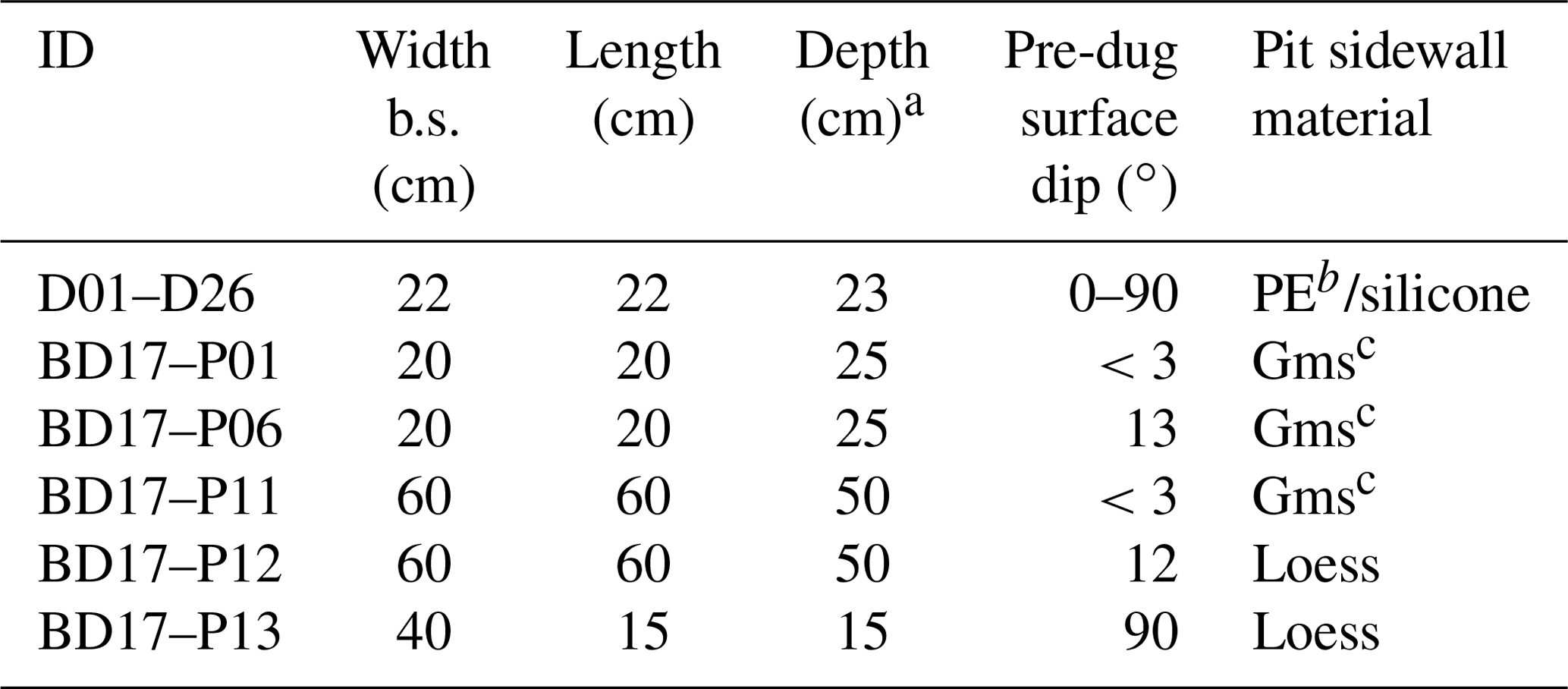
^a Below pre-dug surface. ^b Polyethylene (PE). ^c Matrix-supported gravel.

However, the testing set-up was designed in a way that it would contain features that might play a role during a field campaign and could potentially impede a proper SfM-MVS photogrammetric reconstruction. Examples are steep pit sidewalls, which can also cause strong shading inside the pit and a lack of image texture, for example caused by featureless areas (Gruen, 2012; James and Robson, 2012). For our tests, the latter needed to be improved by painting black/dark brown and white patterns on the flat and initially dark grey sidewalls of the artificial pit and on the pre-dug surface. We further sealed the contact surface between flowerpot and board using white silicone glue. This was necessary in order to be able to determine the reference volume of the test pit by filling it with water, which we repeated 10 times (assuming ${\mathit{\rho }}_{{\mathrm{H}}_{\mathrm{2}}\mathrm{O}}=\mathrm{1}$ g cm⁻³ for demineralised water at ∼20 ^∘C; this assumption holds for all water-based reference volume determinations conducted in this study). An advantage of this type of testing scenario over those used by Bauer et al. (2014) and Berney et al. (2018) is that the test pit could be transported to various locations, simulating different lighting conditions and orientation scenarios. Inside the facilities of the Institute of Geology and Mineralogy at the University of Cologne, images were acquired with artificial lights (ceiling lighting) and/or windows being the main illumination sources. Outside of the facilities, further set-ups included cloudy and sunny conditions, where the pit was either exposed to direct sunlight or in the shade. The pit was also tilted to up to 90^∘, to simulate the sampling of sediment wall faces, i.e. cavities.

In scenarios representing regular pit sampling, i.e. on even or slightly tilted surfaces, typically 24 pictures were taken horizontally in ∼45^∘ steps and vertically at angles of ∼25^∘ (at a height of about 80 cm), ∼50 and ∼90^∘ (both at heights of about 150 cm) to cover all surfaces within the pit; an equal procedure was applied to photograph the pre-dug surface. The distance between the camera lens and the pit was kept constant to make the imagery data as comparable as possible between the sites. For vertical pit volume determinations, imagery was acquired parallel to the surface in an upward/downward and lateral move (about 30 to 40 pictures in total per setting). Additionally, non-surface parallel pictures were taken to image the sidewalls. In general, we aimed to take at minimum three pictures per surface to allow good image matching results (James and Robson, 2012).

In all testing scenarios (including field tests; Sect. 2.2), we used three to four dice on which the dots served as markers and placed three 10 cm long photographic reference scales into the scene. If no ground control points (GCPs) with known reference coordinates are available, the most accurate scaling is achieved by placing a scale that spans over the length of the object of interest (e.g. James and Robson, 2012), as was done by Bauer et al. (2014) and Berney et al. (2018), who placed a frame around the soil pits. In the field, however, when the decision about the extent of a pit may need to be adopted to local constrains (e.g. regolith depth and vegetation cover), such a construction may not be applicable. A further advantage of the photographic reference scales is that they can be used in different (or changing) lighting conditions due to their strong contrasts and that they can be placed at the outer rims and the centre of the respective scene. Pictures were taken initially from the pre-dug surface and afterwards from the pit/cavity to reconstruct a closed and watertight model of the excavation.

Besides using a consumer-grade DSLM camera (Olympus OM-D E-M10, 16 MP (megapixel); Lumix G 50 mm in 35 mm film equivalent f1.7 aspherical fixed-focal-length lens) we also took pictures using the main camera of a Sony Xperia Z5 Compact (23 MP, 24 mm in 35 mm film equivalent f2.0 fixed-focal-length lens). Lens type, dynamic range and image resolution of the DSLM camera used here can be considered to be sufficient for accurate close-range SfM-MVS photogrammetry-based modelling (for an overview on camera hardware requirements see Berney et al., 2018; Eltner et al., 2016; Mosbrucker et al., 2017; Smith et al., 2016). Intentionally, this camera was bought to document geomorphological fieldwork campaigns and not for the purpose of any photogrammetric application. We presume that comparable camera models are currently taken to the field by geoscientists during their TCN sampling campaigns, where impromptu volume determinations of sampling pits may be required. Using the DSLM camera, the pictures were taken in P mode and saved in RAW file format, which preserves a higher information capacity than does the JPEG image format (Mosbrucker et al., 2015). Photographs from the smartphone were taken in manual mode (leaving all settings in automatic mode; Android version 7.1.1) and could only be saved in JPEG file format (highest resolution).

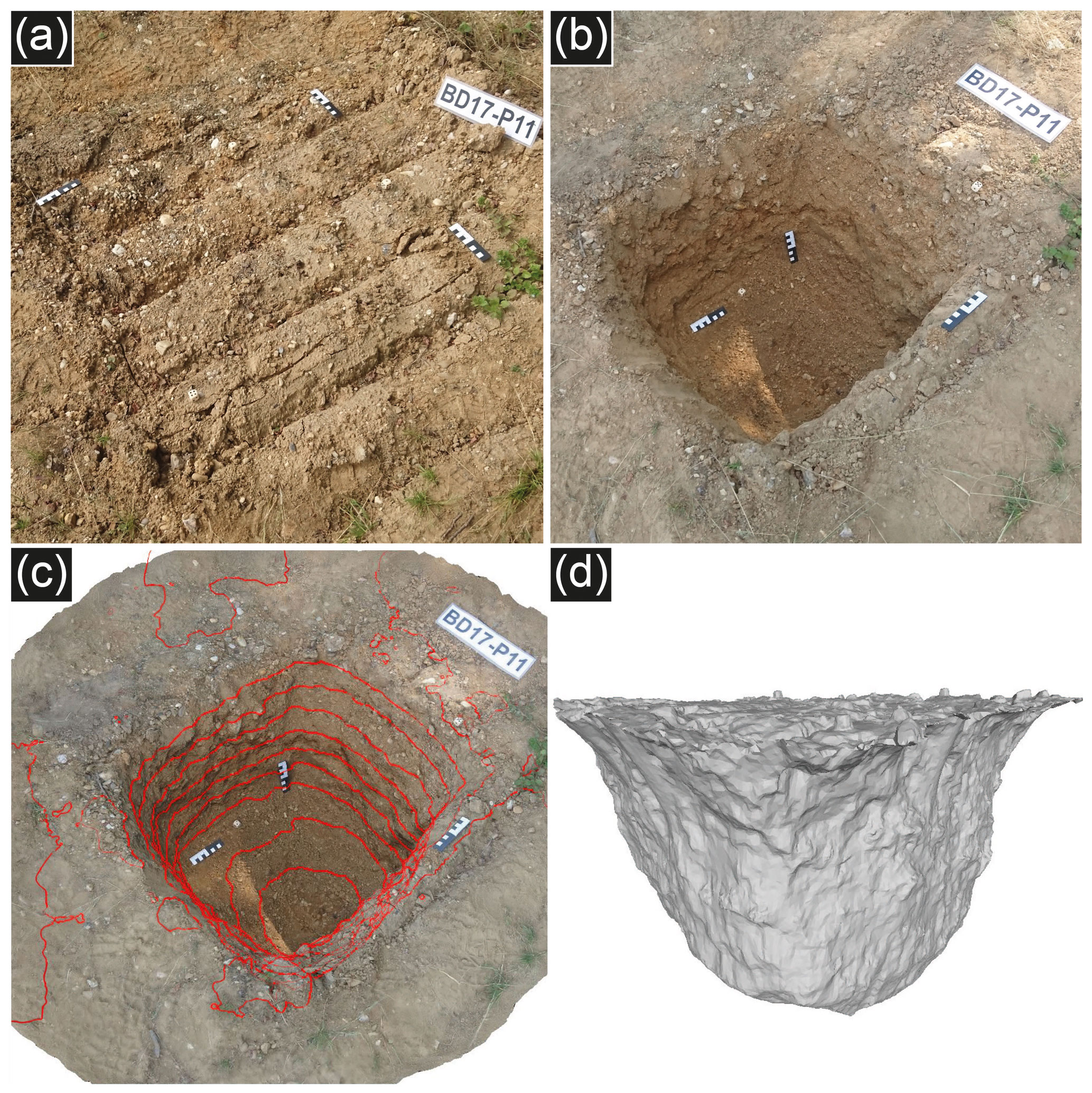
Figure 4 Test site BD17-P11. The pit was dug into gravel situated in a sandy–silty matrix (a, b). The reconstructed pit is shown with 5 cm contours in red (c). The large grain sizes dominating the substrate into which the pit was dug are reflected by the high surface roughness of the final watertight mesh (d).

2.2 Imaging testing scenarios, part 2: field tests

During a second testing phase, a similar imaging using the same cameras was applied for field tests on four soil pits and one loess wall cavity. The field tests were conducted in July 2017 in a gravel pit located approximately 35 km to the west of Cologne, Germany (51.0^∘ N, 6.4^∘ E). Here, gravel belonging to the body of a Middle Pleistocene main terrace of the Rhine River is overlain by a ∼11 m thick sequence of Middle to Late Pleistocene loess deposits and intercalated soils, capped by Holocene soil (Kels, 2007). The gravel is exploited under dry mining conditions. At the outer fringes of the gravel pit, the overburden loess has mostly been removed, leaving the undisturbed uppermost layers of the Pleistocene gravel overlain by a cap of 0 to ∼10 cm of loess. At the outermost rims of the gravel pit, the uppermost ∼4 m of the loess overburden are accessible. As such, the area provides excellent conditions to test the SfM-MVS photogrammetry-based soil bulk density approach on (1) the homogeneous loess and (2) gravel situated in a sandy–silty matrix. Similar to the tests on the artificial pit, this testing environment also provided difficult conditions for the application of the SfM-MVS photogrammetric method, such as potentially disturbing vegetation; heavy shadowing; and – in the case of excavations conducted into the loess – partially low image texture (Gruen, 2012; James and Robson, 2012). Due to the rough surfaces of the sidewalls of the pits dug into the gravel, areas could be shielded from view by protruding clasts and thus not be captured by the photography (Berney et al., 2018). During photographing, weather conditions were mostly sunny but occasionally interrupted by more cloudy episodes (Table 4).

Three pits (BD17-P01, BD17-P06 and BD17-P11) were dug into the gravel (Fig. 4), while BD17-P12 was dug into a ∼12^∘ southward-dipping mine access ramp consisting of compacted loess. All four pits were dug within a radius of ∼20 m. BD17-P13 was dug about 60 m to the north into the foot of a ∼4 m high loess wall. BD17-P01 and BD17-P06 were small pits with a surface area of approximately 20 cm × 20 cm (depth: ∼25 cm), while BD17-P11 and BD17-P12 were about 60 cm ×60 cm in size (depth: ∼50 cm). BD17-P06 was located on a ∼13^∘ eastward-dipping surface. The cavity dug into the loess wall (BD17-P13) measured approximately 40 cm × 15 cm × 15 cm (width × length × depth). All excavations were conducted using a spade and a pickaxe. The excavated material was placed on a tarp, and the mass of both was determined using an ordinary luggage scale (E-PRANCE, max 50 kg, d=0.01 kg). The excavated material of BD17-P01, BD17-P06 and BD17-P13 was also weighted in the laboratory.

From BD17-P11 and BD17-P12 we took pictures during the morning/noon and the afternoon hours to compare the results under different lighting conditions and to assess the reproducibility of the calculated volumes and densities (BD17-P11m, BD17-P11a, BD17-P12m and BD17-P12a). The sampling locations of BD17-P11 and BD17-P12 were chosen in a way that the surrounding vegetation would cause shading of the excavated pit during the afternoon hours. Furthermore, we placed a boulder into these pits to investigate the possibility of detecting the volume change in the respective models (BD17-P11.1m, BD17-p11.1a, BD17-P12.1m and BD17-P12.1a; see Supplement). The reference volume of the boulder (V_b,ref) was determined by submerging it into water, applying Archimedes' principle (six repetitions). To obtain an independent measure of the volume of the excavated pits (the reference volume, V_PU), we filled them using polyurethane foam (PU foam) as described by Brye et al. (2004) and Muller and Hamilton (1992). In addition, polystyrene was used to reduce consumption of the PU foam in the large pits: BD17-P11 and BD17-P12. In the facilities of the UoC, the negative casts were put into watertight bags and submerged under water to determine the respective values for V_PU, applying Archimedes' principle. The cast of BD17-P01 was submerged 11 times, that of BD17-P06 five times and that of BD17-P13 six times to measure the reference volume precision. In addition, we applied the core method by taking volumetric samples (100.0±0.5 cm³) from the larger pits (BD17-P11, n=8 including duplicates; BD17-P12, n=6 including duplicates) and the loess wall (BD17-P13, n=3), using soil sample rings to derive bulk densities independently from the PU-foam/polystyrene-based volume of the excavations (Fig. 2). These samples were oven-dried at 105 ^∘C overnight to constant weights to calculate the dry bulk density ρ_B,d. The excavated material of BD17-P01, BD17-P06 and BD17-P13 was air-dried for several weeks and afterwards treated in a similar fashion as the sample ring samples to derive the dry masses (m_e,d).

2.3 Computer-based workflow

We tested different approaches to derive the SfM-MVS photogrammetry-based pit volumes on the computer. For such computer-based work, three main factors are important to make the method and workflow we test here feasible for a broad range of applications: (1) duration of processing, (2) costs and (3) expertise of the user. As such, we aimed at deriving a workflow that relies entirely (except for the operating system) on freeware computer programs (“freeware workflow”; a detailed protocol on the computing steps is provided in the Supplement) as well as one that might be more convenient to apply but which involves commercial software (“performance workflow”; Fig. 5). Both workflows are based on Windows-compatible computer programs that do not require special knowledge either in programming or in photography and photogrammetry (for a detailed description on the individual computing steps see Smith et al., 2016). The computer we used for testing purposes was a Dell Precision Tower 3620 (3.60 GHz processor, 64 GB RAM, Intel HD Graphics 630 on board and NVIDIA Quadro M4000). Although this machine can be considered to be above average in terms of computing and graphics (year 2020), we note that most processing steps were carried out in the background while working with other memory- and/or graphics-demanding software, such as ArcMap (version 10.6), Google Earth Pro (version 7.3.3) and Microsoft Office 2016.

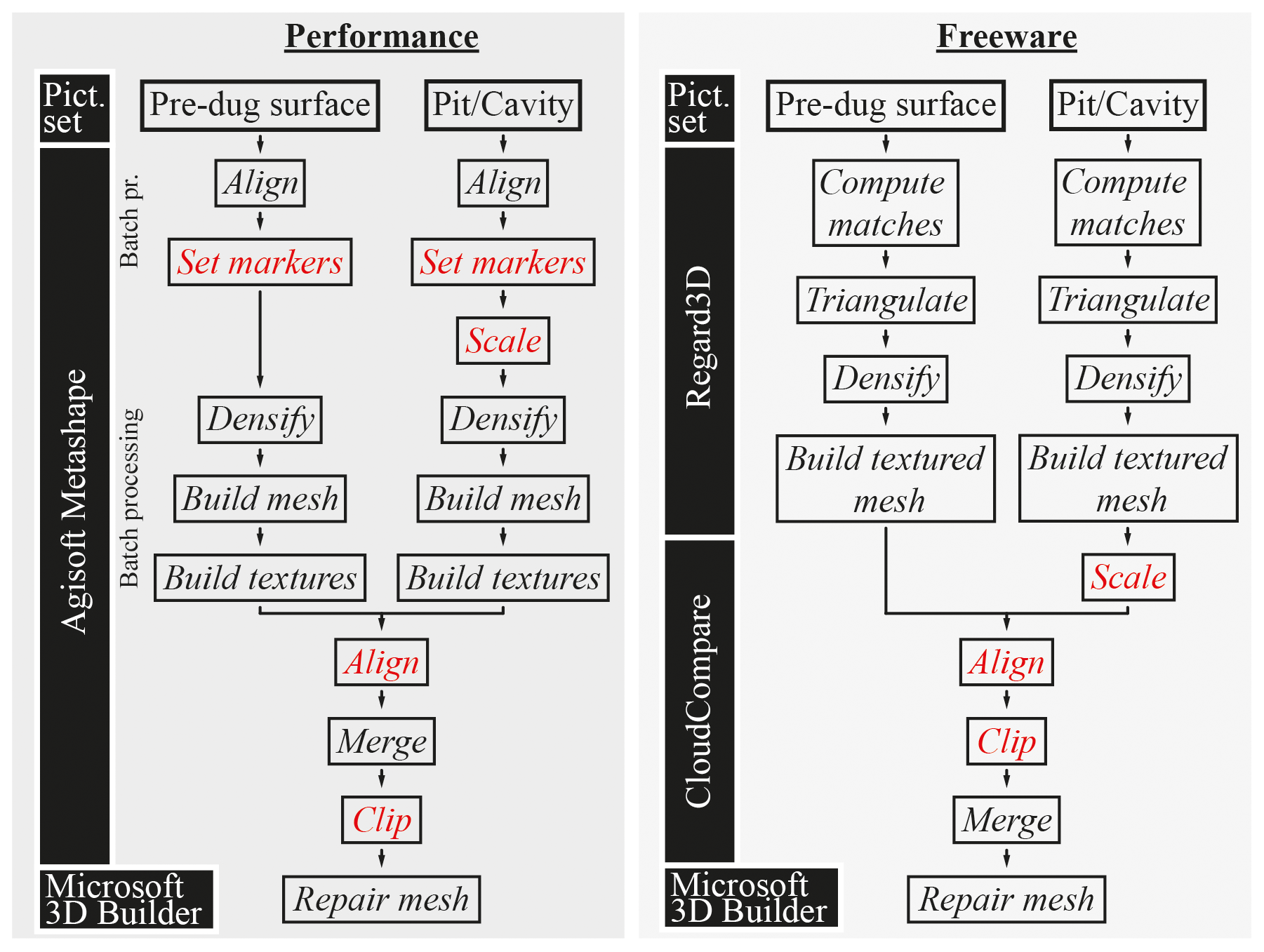
Figure 5 Performance and freeware workflows as applied in this study and the computer programs used. Non- or semi-automated steps are shown in red.

In general, we modelled the pre-dug surface and the pit separately and aligned and merged them afterwards. Watertightness, a prerequisite to deriving the volume of the final model, was achieved by automatically bridging the gaps of the merged mesh. Other approaches, such as deriving a single model from the pre-dug surface and the pit point clouds using the Poisson surface reconstruction (Kazhdan et al., 2006; Kazhdan and Hoppe, 2013), led to the appearance of large bumps in the model if the surface roughness of the pit was too high. For example, Poisson surface reconstruction did not create an accurate but bumpy surface of the boulder placed into the pits of scenarios BD17-P11.1 and BD17-P12.1, most likely due to bad orientation of the face normals. In addition, various manual adjustments were required, such as a re-orientation of face normals, to get appropriate results even for easier-to-model settings. Thus, we chose to reconstruct the pre-dug and the pit surfaces parallel and merged the final meshes afterwards. The model outcomes were visually checked for irregularities such as uneven surfaces, holes and bumps. As long as these features did not reflect large deviations from the reference shape, we accepted the respective model for further data analysis.

For the freeware workflow, we used the programs Regard3D (version 1.0.0) to build point clouds and meshes and CloudCompare (version 2.11) to scale the pit model and to align and merge it with the pre-dug surface (for an overview on other photogrammetry software available see Eltner et al., 2016; Smith et al., 2016). We chose these programs because we find them straightforward to use and both come with comprehensive documentation. All the steps listed above can be carried out in Agisoft Metashape Pro (version 1.6.1), which is the main (commercial) program used in the performance workflow and which has been widely used for applications in geoscience (Eltner et al., 2016). The software also allows for batch processing and supports graphics processing unit (GPU) acceleration. For all modelling performed in this study using Agisoft Metashape Pro, we used either the integrated (testing scenarios) or the additionally installed (AT17–18 sampling campaign, Sect. 2.4) graphics card for GPU acceleration.

In both the performance and freeware workflows, the final step was to bridge the edges of the reconstructed pre-dug surface and the pit to water-tighten the models, which was achieved using Microsoft 3D Builder (version 18.0.1931.0). Regard3D requires pictures in the JPEG file format as input, while Agisoft Metashape can process TIF files, which contain a higher information capacity than do JPEG files (Mosbrucker et al., 2015). The images taken using the DSLM camera in the RAW file format were converted accordingly. While running both workflows, we recorded the time that was required to finally determine the volume (using e.g. CloudCompare or MeshLab, version 2016.12). Photographs were not post-processed (an overview on some possibilities for post-processing are summarised in Mosbrucker et al., 2017) before using them for the SfM-MVS photogrammetric reconstruction to keep the workflow as simple as possible.

We always aimed at leaving the default parameters for the respective processing steps, which worked fine in the majority of the cases, especially for the field tests. This included Poisson surface reconstruction octree depth (Kazhdan et al., 2006; Kazhdan and Hoppe, 2013) in Regard3D (default: 9) and the cloud densification/meshing accuracy (default: medium) in Agisoft Metashape, mainly because meshes generated from both the freeware and the performance workflow would be comparable in detail and file size (in general <10 MB). Agisoft Metashape is able to automatically detect markers placed within a given set of aligned photographs. For the tests on the artificial pit using the smartphone camera (D17 to D26), we thus marked the photographic reference scales with pairs of black circles, located at a known distance from each other, to test if this could speed up the processing.

2.4 Soil bulk density transects from the Altos de Talinay, northern central Chile

The experience obtained during the testing phase was important in applying SfM-MVS photogrammetry for expedient soil bulk density analysis along N–S-oriented TCN sampling transects spanning the slopes of three E–W-running valleys (C1, C2 and C5; Fig. 9) in the Altos de Talinay. Geographically, the study area is part of the Coastal Cordillera of northern central Chile (30.5^∘ S, 71.7^∘ W). The main aim of the TCN sampling campaign, which was conducted in March 2018, was to derive process rates (erosion and soil production; e.g. Dunai, 2010; Heimsath and Jungers, 2013) from concentrations of cosmogenic nuclides in sediments and bedrock/saprolite. In this generally arid to semi-arid study area (e.g. Gutierrez et al., 2010; López-Cortés and López, 2004), north-facing slopes (NFSs) tend to be flatter and less densely vegetated then their south-facing counterparts (SFSs), which show greater regolith depths and are generally subject to intense bioturbation (cf. Gutiérrez-Jurado and Vivoni, 2013a, b). The type of vegetation differs between xeric shrubland on the NFS and evergreen sclerophyll shrubs on the SFS (Armesto and Martnez, 1978; and own observations). The major soil types found in the study area are Entisols and Aridisols (Casanova et al., 2013). The soils are situated on intrusive rocks (melanocratic facies containing dioritic protolith rocks, intruded by leucocratic granitoid dikes; Emparan and Pineda, 2006; Gana, 1991; and own observations) with a mean density ρ_BR of 2.82±0.11 g cm⁻³, as measured by submerging bedrock and unweathered saprolite samples (n=28) from catchment C5 under water.

We obtained soil density data from in total 69 soil pits dug into diffusively eroding slope noses and ridgetops, using a spade, a hand shovel and a pickaxe. The soil pits were located within a distance of about 25–50 m from each other. As soil bulk densities are strongly influenced by biotic activity and plant cover, among other factors (for an overview see e.g. Al-Shammary et al., 2018, and references therein), the densities as measured using the SfM-MVS photogrammetry-based technique should reflect aspect-related differences in the study area. To acquire the imagery, we used two different DSLM cameras: the Olympus E-M10 (14–42 mm f3.5–5.6 lens, pictures mostly taken at 14 mm, i.e. 28 mm in 35 mm film equivalent), which was also used in the tests described in Sect. 2.1.1 and 2.1.2 with a different lens, and a Panasonic DMC-GX80 (16 MP; Lumix G 40 mm in 35 mm film equivalent f1.7 aspherical fixed-focal-length lens). Automatic mode was used for both cameras when taking the pictures, which were saved in JPEG file format (highest resolution). The imaging technique was based on the experiences made during the test phase, so we took care to cover all surfaces at least three times and included close-ups (avoiding using optical zoom; e.g. Smith et al., 2016). To enhance the image texture, a brush was used to clean the bedrock/saprolite layer at the bottom of the respective pit. At most sites, three to four dice and two to three scale bars were placed for referencing and scaling purposes. Weather conditions were either sunny or cloudy; photographs were taken between 10:30 and 18:30 LT. Similar to the BD17 field tests, the excavated material was put on a tarp to measure its weight using a hand balance (KERN 50K50, d=50 g). The weight of the tarp was later subtracted from the final mass of the excavated material (m_e,f). All computing steps were conducted using a Gigabyte Z87-D3HP-based computer (3.10 GHz processor, 16 GB RAM, Intel HD Graphics 4600 on board and NVIDIA GeForce GTX 760) with no other memory- and/or graphics-demanding software running simultaneously.

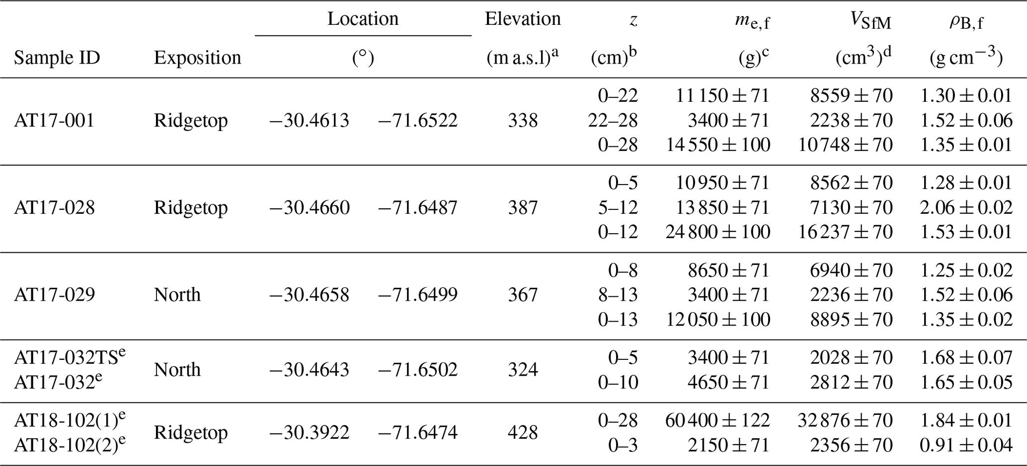
Although we tested the accuracy and precision of the SfM-MVS photogrammetry-based density estimation before this fieldwork was conducted, we decided to further test the reliability of the technique in the field by a stepwise volume determination in three pits (AT17-001, AT17-028 and AT17-029; all pictures used to derive soil bulk densities in this study were taken during March 2018). In detail, we dug the pit until the saprolite or bedrock was reached and applied the usual workflow to measure the weight of the excavated material and to take the pictures needed for the photogrammetric reconstruction. In the case of a stepwise volume determination, we then further dug into the saprolite, again weighing the mass of the excavated material and taking another set of pictures from the deepened pit. This method allowed for the photogrammetric reconstruction of three models: (1) the shallow pit, (2) the deepened pit and (3) the “void” between the ground surfaces of the shallow and the deepened pits. By applying the performance workflow to all three models independently from each other, we could test if the volume determination is internally consistent, i.e. if the sum of the volumes of (1) and (3) equals the total volume of (2).

In addition to these tests, we dug two pits located close to each other (∼1 m) but reaching different depths into the regolith layer in order to compare their values for ρ_B,f. We expected these to be similar in the weakly developed soils of the study area (AT17-032, 10 cm; AT17-032TS, 5 cm). A similar approach was applied at sample sites AT18-102(1) and AT18-102(2), where we dug 28 cm (soil–saprolite mix) and 3 cm (soil only) into the ground, respectively. Here, our intention was to test if a clear and significant change in density could be measured.

For most sampling sites where we took our TCN samples, we also aimed at sampling a small (∼330 g on average) but representative column of regolith covering the entire profile of the respective pits. This material was used to assess the gravimetric water content and the mass of the fraction >2 mm of the soils. Soil densities are affected by the water content of the soil and the presence of larger clasts in the sample and are thus commonly corrected for both variables by drying the samples and removing the >2 mm fraction in order to measure dry soil densities (ρ_d; e.g. Blake and Hartge, 1986; Soil Survey Staff, 2014). Although the determination of ρ_B,f is likely sufficient for a correction of TCN production rates in arid zones, in some cases it might be necessary to infer ρ_B,d, especially if the samples were taken during the wet season. In addition to that, the method might also be used to infer comparable values of ρ_d in non-TCN-related applications. Thus, we used the aliquot samples to calculate the conversion factors f_d (conversion to calculate the oven-dried mass of the excavation as applied by Blake and Hartge (1986) for the clod method), f_r,d (conversion to remove the mass of the >2 mm fraction from the oven-dried excavated mass) and f_r,V (conversion to remove the volume of the >2 mm fraction from the excavated volume),

$$\begin{array}{}\text{(3)}& {\displaystyle }& {\displaystyle }{f}_{\mathrm{d}}=m_{\mathrm{a},\mathrm{d}}{m}_{\mathrm{a},\mathrm{f}}^{-\mathrm{1}},\text{(4)}& {\displaystyle }& {\displaystyle }{f}_{\mathrm{r},\mathrm{d}}=\mathrm{1}-\left(m_{\mathrm{a},\mathrm{r}}{m}_{\mathrm{a},\mathrm{d}}^{-\mathrm{1}}\right),\text{(5)}& {\displaystyle }& {\displaystyle }{f}_{\mathrm{r},\mathrm{V}}=\mathrm{1}-\left[V_{\mathrm{a},\mathrm{r}}{\left(m_{\mathrm{a},\mathrm{d}}{\mathit{\rho }}_{\mathrm{B},\mathrm{d}}^{-\mathrm{1}}\right)}^{-\mathrm{1}}\right],\end{array}$$

with m_a,f being the field-state mass of the aliquot sample, m_a,d its oven-dried mass, m_a,r the mass of the fraction >2 mm and V_a,r the volume of the rocks in the aliquot sample (cf. Russo, 1983; Soil Survey Staff, 2014; Vincent and Chadwick, 1994). V_a,r could either be measured, for example by submerging the clasts under water, or derived by using the bedrock density ρ_BR, which would equal the assumed density of the clasts (Brye et al., 2004; Grossman and Reinsch, 2002; Russo, 1983; Vincent and Chadwick, 1994). While Eq. (4) assumes that the >2 mm fraction is free of moisture, Eq. (5) assumes that the clasts in the soil pits are separated by <2 mm material or contact between the >2 mm clasts is minimal (Grossman and Reinsch, 2002). To ensure that water loss after sampling would be minimised (e.g. Blake and Hartge, 1986), the sampling material of the aliquots (n=37) was sealed in plastic bags and stored at a cool and shaded place during fieldwork and in an air-conditioned room afterwards. Further processing – i.e. drying, sieving, weighing and determining V_a,r by submerging the clasts in a water-filled volumetric flask – was performed in facilities of the Universidad Católica del Norte (UCN), Antofagasta, Chile. With regard to the general formula for ρ, defined as mass per volume, inserting Eq. (3) in Eq. (2) yields

$$\begin{array}{}\text{(6)}& {\mathit{\rho }}_{\mathrm{B},\mathrm{d}}=\left(m_{\mathrm{e},\mathrm{f}}{m}_{\mathrm{a},\mathrm{d}}{m}_{\mathrm{a},\mathrm{f}}^{-\mathrm{1}}\right)V_{\mathrm{SfM}}^{-\mathrm{1}}\end{array}$$

to approximate the dry bulk density. Accordingly, the dry soil density can be approximated by inserting Eqs. (3)–(5) into Eq. (2), yielding

$$\begin{array}{}\text{(7)}& \begin{array}{rl}{\mathit{\rho }}_{\mathrm{d}}=& \left[\left[\left(m_{\mathrm{a},\mathrm{d}}-m_{\mathrm{a},\mathrm{r}}\right)m_{\mathrm{a},\mathrm{f}}^{-\mathrm{1}}\right]m_{\mathrm{e},\mathrm{f}}\right]\\ & {\left[\mathrm{1}-\left[V_{\mathrm{a},\mathrm{r}}{\left(m_{\mathrm{a},\mathrm{d}}{\mathit{\rho }}_{\mathrm{B},\mathrm{d}}^{-\mathrm{1}}\right)}^{-\mathrm{1}}\right]V_{\mathrm{SfM}}^{-\mathrm{1}}\right]}^{-\mathrm{1}}\end{array}\end{array}$$

and thus providing the possibility to approximate comparable soil densities using a combination of the SfM-MVS photogrammetry-based method and representative regolith sampling.

3 Results

3.1 Volume inferences from the artificial pit

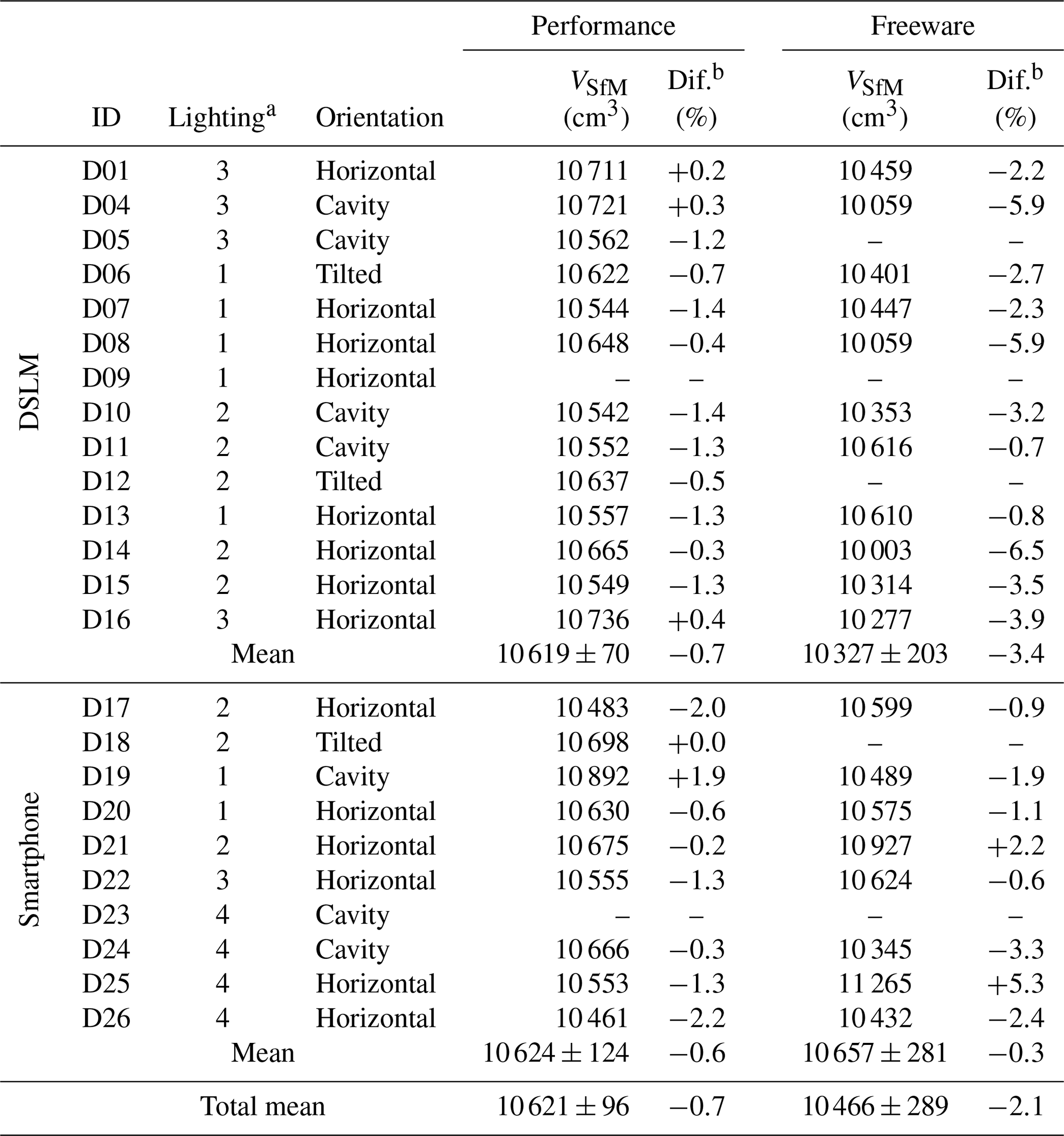
In total, 16 settings were photographed using the DSLM camera, and 10 settings using the smartphone (Fig. 6, Table 2). For all scenarios but two (D09 and D23), the applied performance workflow yielded visually matching modelling reproductions of the inside of the flowerpot. Regarding the freeware workflow, default processing settings had to be adjusted in the majority of cases to generate the surfaces. This predominantly applied to the point cloud densification step of the pits in Regard3D, which was mostly carried out using the multi-view environment (MVE) method (Fuhrmann et al., 2014) instead of the default patch-based and clustering multi-view stereo algorithms (CMVS/PMVS; Furukawa and Ponce, 2009). The latter often failed to densify the point cloud in shady and/or dark areas of the artificial pit. In 19 out of 41 successfully created models Netfabb Basic (freeware; version 7.4.0) had to be used to bridge one edge of pre-dug surface to an edge of the pit mesh manually (<1 min of additional processing time required). This step was necessary in cases where the meshes of pre-dug surface and pit did not overlap at any point, i.e. where no connection was established beforehand. However, five freeware scenarios (D05, D09, D12, D18 and D23) failed to yield acceptable watertight meshes. For scenarios where the modelling was successful, the derived volumes differed on average by about −0.7 % (performance, DSLM), −0.6 % (performance, smartphone), −3.4 % (freeware, DSLM) and −0.3 % (freeware, smartphone) from the respective reference volumes. The maximum recorded difference was −6.5 %, calculated for D14 applying the freeware workflow.

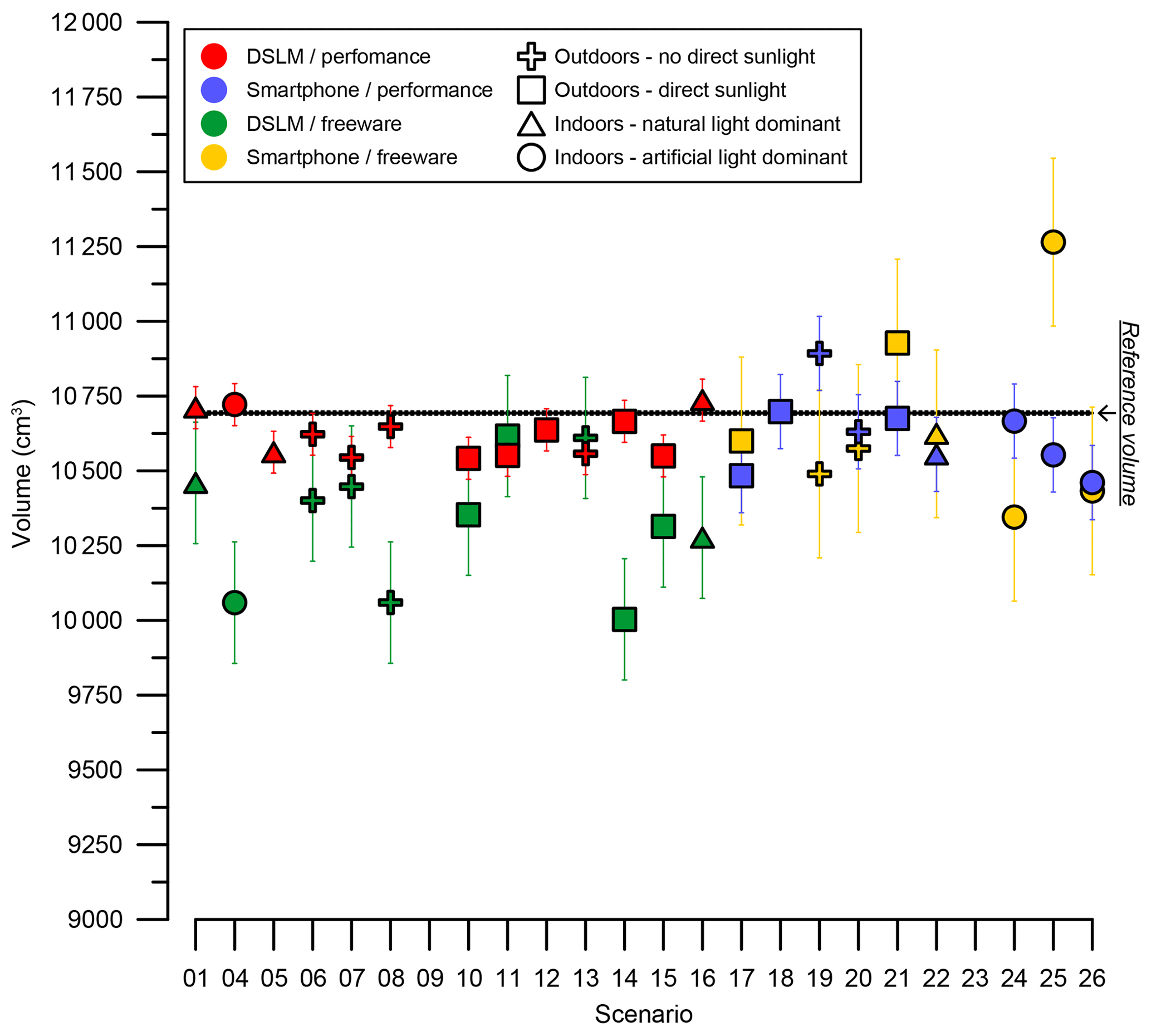
Figure 6 Performance- and freeware-workflow-derived SfM-MVS photogrammetric volumes of the artificial pit using a DSLM and a smartphone camera for different settings and lighting conditions. The reference volume (solid black line with dashed black error range) of 10 693±7 cm³ was measured by filling the empty flowerpot with water and recording the difference in weight (assuming ${\mathit{\rho }}_{{\mathrm{H}}_{\mathrm{2}}\mathrm{O}}=\mathrm{1}$ g cm⁻³ for demineralised water at ∼20 ^∘C water temperature).

Table 2 Scenario details and derived volumes (V_SfM) of the artificial pit by applying the performance and freeware workflows.

^a Lighting conditions as follows: 1 – outdoors, little or no direct sunlight (i.e. shady or cloudy); 2 – outdoors, direct sunlight; 3 – indoors, sunlight as the main illumination source; 4 – indoors, artificial light (ceiling lighting) as the main illumination source. ^b Difference between the modelled volume and the reference volume (10 693±7 cm³).

In general, the volumes derived using this workflow showed a lager variability (203 cm³ using the DSLM and 281 cm³ using the smartphone) than the performance workflow (70 cm³ using the DSLM and 124 cm³ using the smartphone). Average processing durations ranged between 25 and 30 min for all workflows and cameras applied (see Table B1). However, the effective time of non-automated, i.e. manual, processing was twice as long for the performance workflow (∼15 min) as for the freeware workflow (8 min). A clear advantage of the performance workflow is the ability to perform batch processing in Agisoft Metashape, while attendance of the user is required after each processing step in Regard3D.

3.2 Volumes and densities obtained from the field tests

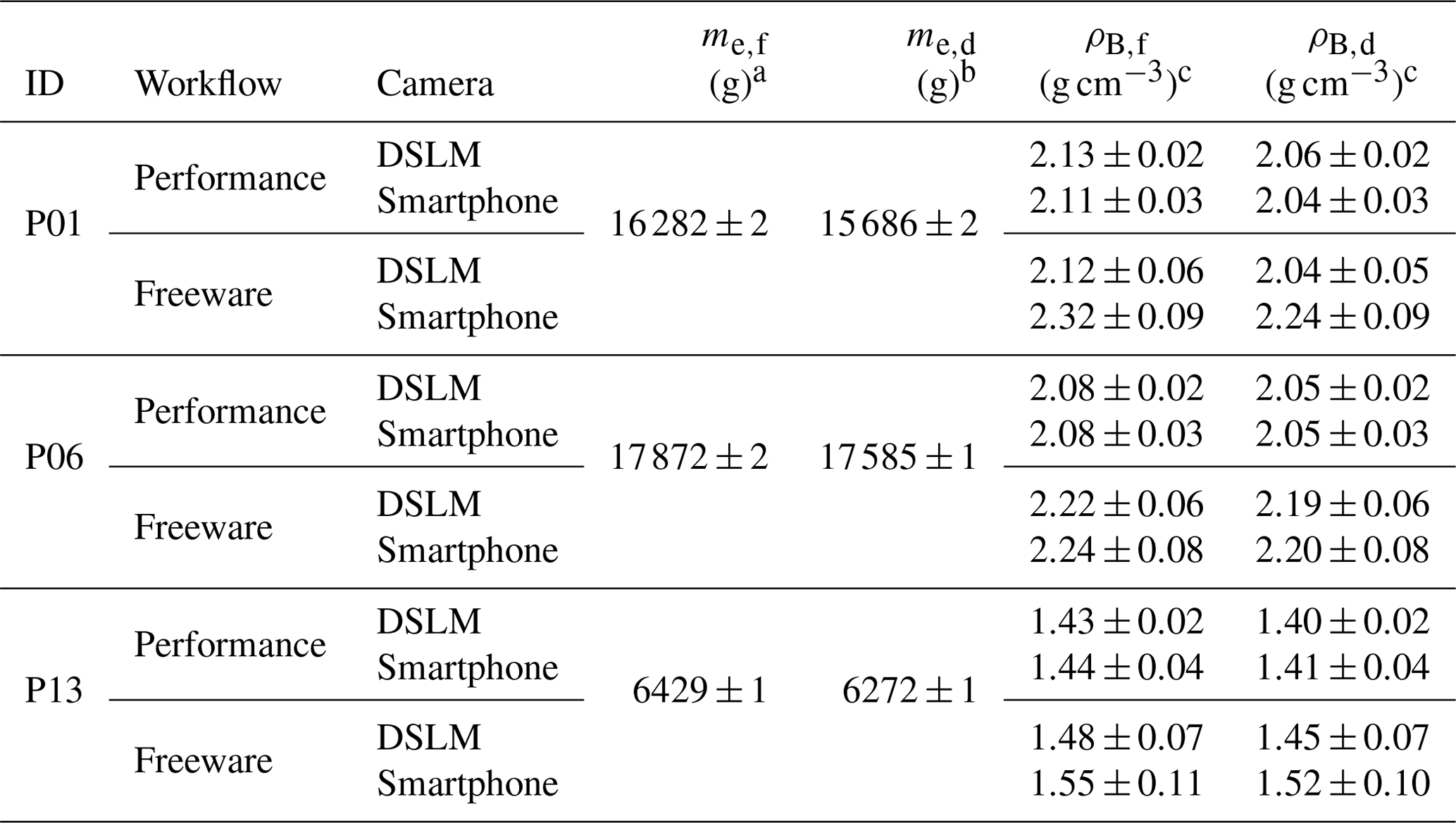
The reference PU-foam-based method (Sect. 2.2) yields consistent field-state bulk densities for BD17-P01 and BD17-P06 (∼2.12 g cm⁻³; Table 3). The highest value of ρ_B,f is measured for BD17-P11 (2.34±0.01 g cm⁻³). In contrast to that, lower values are obtained for the loess pit BD17-P12 (1.90±0.01 g cm⁻³) and the loess cavity BD17-P13 (1.54±0.03 g cm⁻³). PU-foam/polystyrene-derived field densities significantly differ from those derived using soil sample rings (Table B3) in two out of three sites. Only at site BD17-P12 do the respective values (PU foam: 1.90±0.01 g cm⁻³; sample rings: 1.82±0.08 g cm⁻³) overlap. However, close values are also obtained for site BD17-P13, especially when the oven-dried masses m_e,d (dried excavation) are used to calculate ρ_B,d (PU foam: 1.51±0.03 g cm⁻³; sample rings: 1.35±0.09 g cm⁻³). V_b,ref was measured to be 6116±63 cm³. We subtracted this value from the PU-foam-cast-derived measurements of sites P11 and P12, yielding volumes of 93 789±326 and 88 959±326 cm³, respectively (error propagation in this study by adding uncertainties in quadrature).

Table 3 Reference volumes (V_PU), excavation masses (field state – m_e,f; dry – m_e,d) and densities (field state – ρ_B,f; dry – ρ_B,d) obtained from the BD17 test sites.

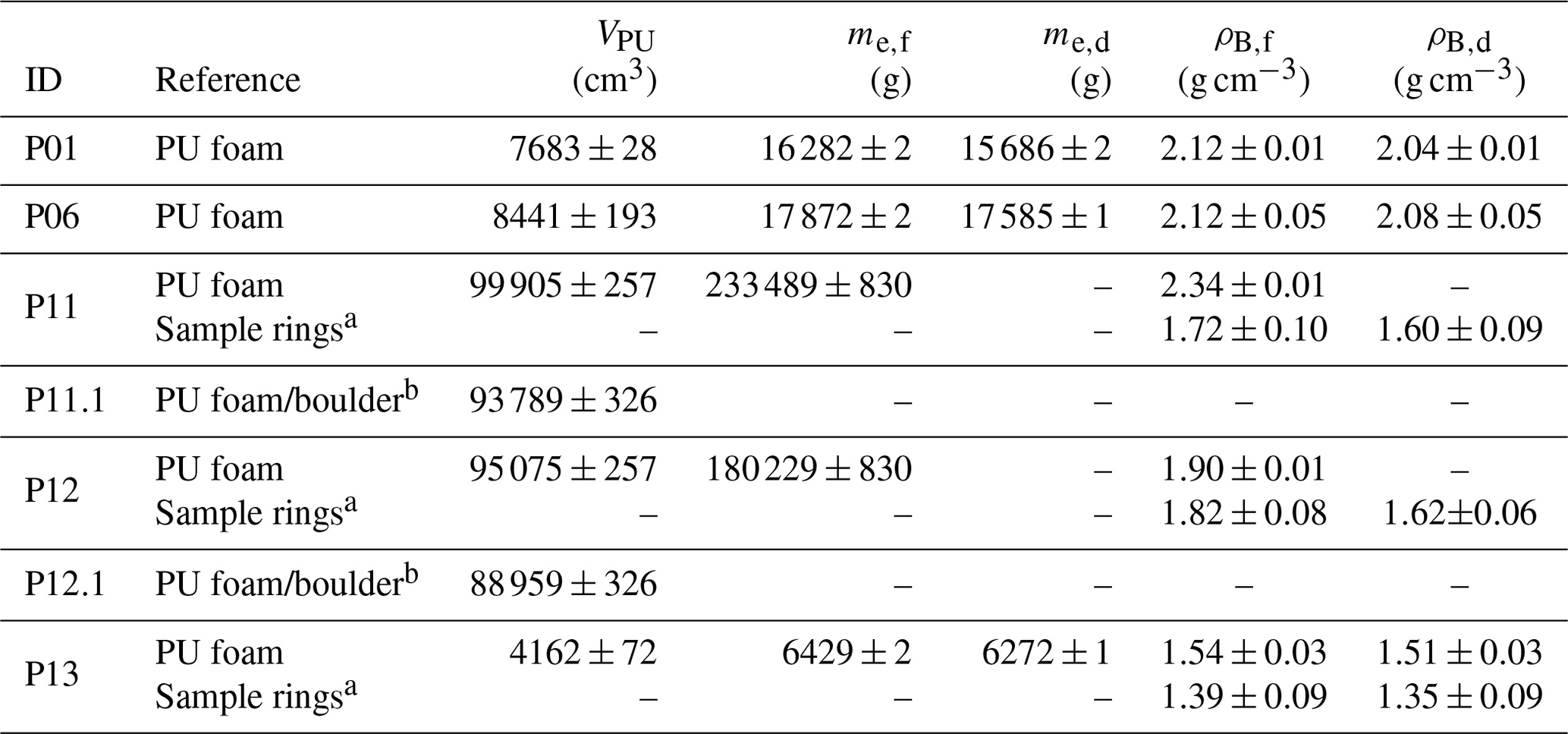
^a Mean values of multiple (BD17-P11: 8; BD17-P12: 6; BD17-P13: 3) measurements using 100 cm³ soil sample rings. ^b Volume of a boulder (6116±63 cm³) placed into the respective pits subtracted from PU-foam-derived volume.

Concerning the SfM-MVS photogrammetry-based pit reconstructions, modelled volumes show a high correlation with the reference volumes (R²=0.98; Fig. 7). For the pits BD17-P01, BD17-P06, BD17-p11, BD17-P12 and BD17-P13, the deviations from the reference volumes range between −8.7 % and +13.8 % (Table 4). Sixteen out of 28 modelled volumes differ by less than 5 % from the respective reference values. In most cases, the freeware workflow yields the largest deviation within a given setting (BD17-P01, BD17-P06, BD17-P11a and BD17-P12). In all settings except for BD17-P11, the difference is below 8 %. Like at most other sites, the large deviations in that particular setting show little variabilities (+8.2 % to +11.1 % for P11m and +10.5 % to +13.8 % for P11a).

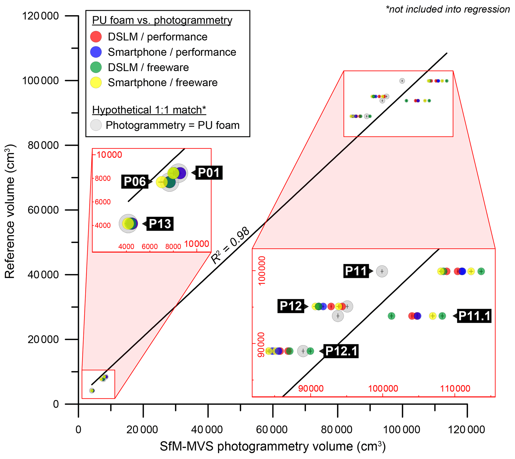
Figure 7 Pit (BD17-P01 to BD17-P12.1) and cavity (BD17-P13) volumes derived using PU foam/polystyrene casts (reference volumes) and the SfM-MVS photogrammetry workflows tested in this study. Hypothetically matching values obtained from the PU foam/polystyrene casts are indicated by large grey circles (errors of these values on the ordinate reflect measurement standard deviations; errors on the abscissa reflect the standard deviation of all photogrammetric reconstructions as determined on the artificial pit, i.e. ∼169 cm³; Table 2). For discussion, see text.

Table 4 Imaging scenarios, photogrammetry-derived volumes (V_SfM), excavation weights (field state; m_e,f) and field bulk densities (ρ_B,f) of the standard pits BD17-P01, BD17-P06, BD17-P11, BD17-P12 and BD17-P13.

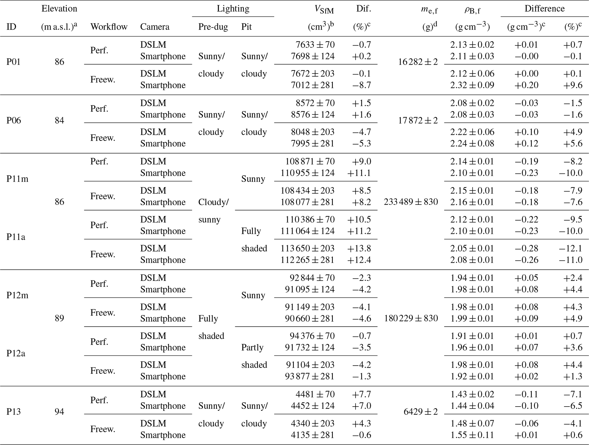
^a All samples taken within a radius of ∼50 m (50.9972^∘ N, 6.4345^∘ E). ^b Uncertainties are 1σ as obtained from the tests performed on the artificial pit (see Table 2). ^c Difference between modelled volumes/densities and reference values (see Table 3). ^d Errors based on balance accuracy. The accuracy of the hand balance used here to lift the excavated material of BD17-P11 and BD17-P12 and the tarp was determined to be about ±260 g by comparing test measurements with those obtained from an ordinary balance (d=1 g) in the laboratories of the University of Cologne. The latter balance was further used to determine the mass of the excavations of BD17-P01, BD17-P06 and BD17-P13.

As indicated by the results obtained from the tests using the artificial pit, volumes based on images taken from the DSLM and the smartphone are very consistent when the performance workflow is applied. Consequently, calculated densities are very similar at each site (average difference is ∼0.02 g cm⁻³); DSLM–freeware- and smartphone–freeware-workflow-derived densities are slightly less consistent (average difference ∼0.04 g cm⁻³).

The reconstruction of the modified pits BD17-P11.1 and BD17-P12.1 yielded more accurate and precise results for the performance workflow than for the freeware workflow (Table 5). Mean values for the boulder (V_b,sfm), calculated by subtracting the volumes of the standard pits from the corresponding modified pits, are 6262±1300 g cm⁻³ (DSLM imagery) and 6264±97 g cm⁻³ (smartphone photographs; here, errors represent the standard deviation of the mean without including measurement uncertainties). In contrast to that, mean freeware-based volumes are 4450±2199 and 6842±2012 g cm⁻³ for DSLM and smartphone images, respectively.

Table 5 Imaging scenarios and SfM-MVS photogrammetry-derived volumes of the modified pits BD17-P11.1 and BD17-P12.1 (V_SfM) and the resulting boulder volumes (V_b,SfM).

^a Uncertainties are 1σ as obtained from the tests performed on the artificial pit (see Table 2). ^b Difference between modelled volumes/densities and reference values (see Table 3). ^c Reference volume calculated by subtracting the reference value for V_b,ref (6116±63 cm³) from the PU-foam/polystyrene-cast-derived reference volumes V_PU. ^d Derived by subtracting the volumes of the standard pits from the corresponding modified pits. ^e Not determined.

The large differences between the modelled volumes of BD17-P11 and the corresponding values for V_PU are also reflected in the final values for ρ_B,f (Fig. 8). Deviations from the reference range between −0.18 and −0.28 g cm⁻³, with the latter being the maximum difference recorded in this test. Fifteen out of 28 calculated densities differ by less than 0.1 g cm⁻³ from the reference density. The average difference is lowest for the DSLM–performance workflow (0.09 g cm⁻³) and the smartphone–performance workflow (0.11 g cm⁻³). The DSLM–freeware and smartphone–freeware workflows yield average differences of 0.12 and 0.13 g cm⁻³, respectively. However, these values are strongly affected by generally large deviations reported for site BD17-P11. If only the remaining sites (BD17-P01, BD17-P06, BD17-P12 and BD17-P13) are considered, mean differences decrease to 0.05 g cm⁻³ (DSLM–performance) and 0.06 g cm⁻³ (all others). The application of sample rings generally yielded lower densities than the SfM-MVS photogrammetry-based densities (Tables 3 and 4). However, the obtained mean values are very similar to those derived using SfM-MVS photogrammetry and partially overlap within their error ranges at sites BD17-P12 and BD17-P13. Using the m_e,d to calculate ${\mathit{\rho }}_{\mathrm{B},\mathrm{d},}$, densities decrease by about 0.08 g cm⁻³ (BD17-P01), 0.03 g cm⁻³ (BD17-P06) and 0.04 g cm⁻³ (BD17-P13) (see Table B2).

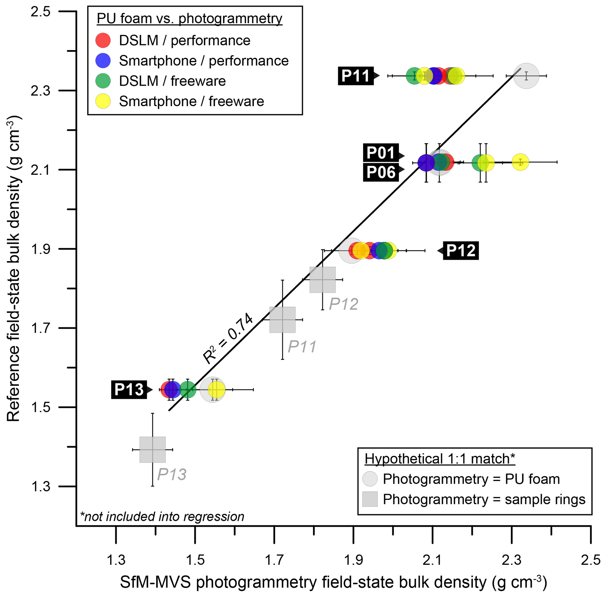
Figure 8 Pit (BD17-P01 to BD17-P12) and cavity (BD17-P13) densities derived using PU foam/polystyrene casts (reference densities) and the photogrammetry workflows presented in this study. Hypothetically matching values obtained from the PU foam/polystyrene casts and soil sample rings are indicated by large grey circles and squares (errors on the ordinate reflect measurement standard deviations; errors on the abscissa reflect the standard deviation of all photogrammetry-based densities for the respective sites). For discussion, see text.

It took on average 53 min from uploading the pictures to obtain the final pit volume when the DSLM–performance workflow was applied and 68 min for the smartphone–performance workflow (see Table B1). This was faster than the average durations recorded for freeware workflows (85 min using the DSLM pictures and 86 min using the smartphone pictures). A regularly applied deviation from the default settings of the freeware workflow was the adjustment of the matching key point sensitivity in Regard3D, which in most cases had to be lowered to save computing time. In the case of the modified pits BD17-P11.1 and BD17-P12.1, three to nine additional pictures taken from different horizontal angles (but same distance to the object) had to be added in order to reconstruct the shape of the boulder placed inside the respective pits more properly.

As already noted for the tests carried out using the artificial pit, the working steps requiring intensive manual adjustments took less time for the freeware workflows (17 min on average) than the performance workflows (26 min using the DSLM pictures and 32 min using the smartphone photographs).

3.3 Altos de Talinay sampling transects

During the fieldwork conducted in March 2018, we took on average ∼50 pictures per site (n=69; see Supplement). In contrast to the image acquisition as conducted during the test phase, when an equal amount of pictures were taken from the pre-dug surface and the pit (about 50–60 pictures per site in total), we mainly focused on the pit as it has been shown to be not only more important but also more difficult to reconstruct. However, 30 or fewer pictures in total was also sufficient to generate watertight models accurately reflecting the original pit.

On average, mean processing durations (57 min to obtain one density value) were close to those reported for the BD17 field tests (DSLM–performance workflow; see Table B1). Difficulties during processing mainly arose during the alignment of the pre-dug surface mesh and the pit model, if the ground had not been sufficiently cleared from vegetation before the pit was dug or if the radius of clearance work around the pit was not large enough. In these cases the (manual) scanning for matching reference points was complicated in both models; the contribution of this step to the total processing time consumption was on average 11 min (19 %), a bit higher than recorded for the BD17 field test (8 min or 15 % for the DSLM–performance workflow).

The stepwise volume quantification of the three test sites yielded deviations of +49 cm³ (AT17-001), −545 cm³ (AT17-028) and +280 cm³ (AT17-029) when compared to the total volume obtained from the finally deepened pit (Table 6). The resulting differences in ρ_B,f would be 0.01 g cm⁻³ for AT17-001, 0.05 g cm⁻³ for AT17-028 and 0.04 g cm⁻³ for AT17-029. The duplicate soil densities analysed in pits AT17-032 and AT17-032TS are very similar (1.65±0.05 cm⁻³ and 1.68±0.07 g cm⁻³, respectively), while the density of the soil–saprolite mix of AT18-102(1) is twice as large as that of the soil layer in AT18-102(2) alone (1.84±0.01 g cm⁻³ vs. 0.91±0.04 g cm⁻³).

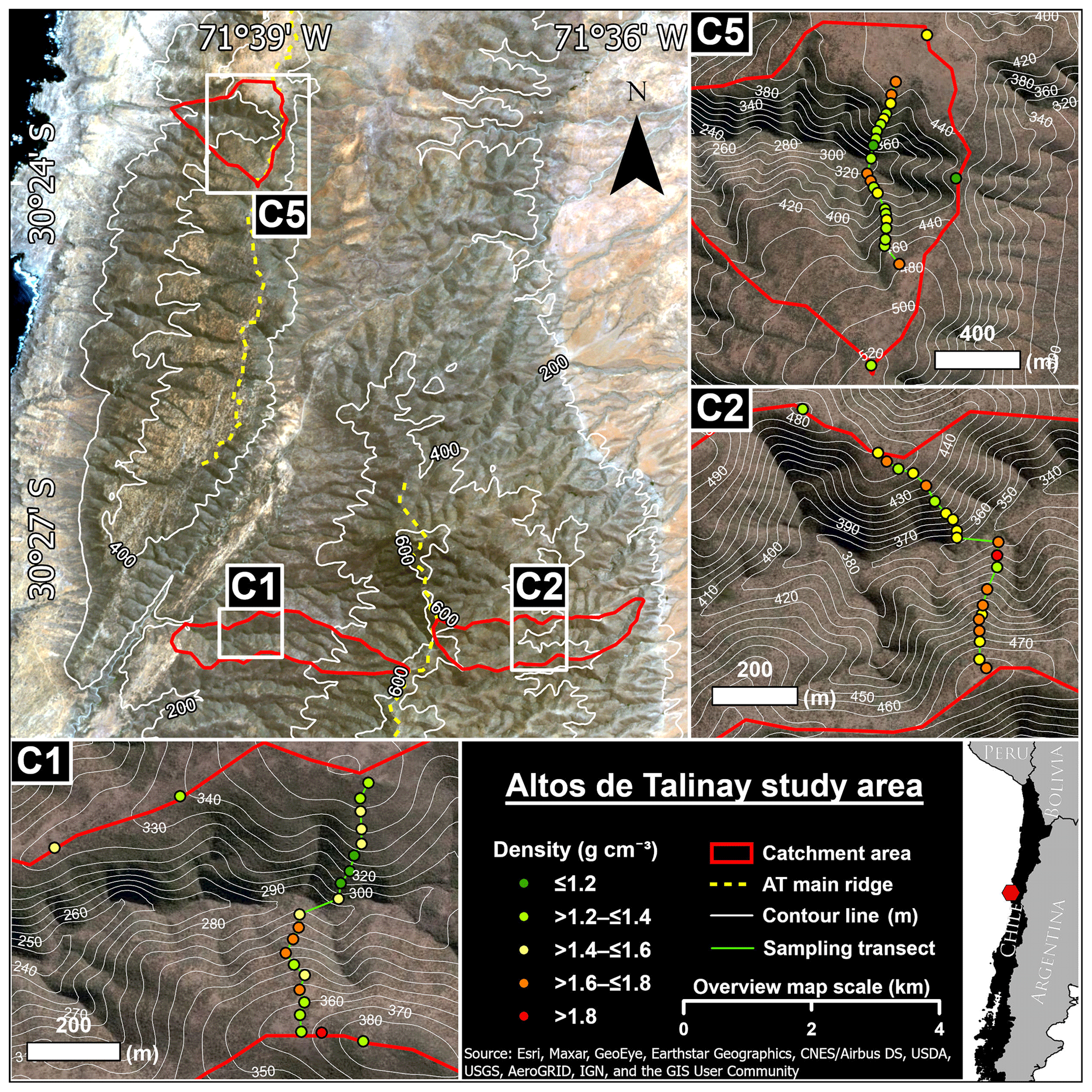
Figure 9 Sentinel 2B satellite image showing the location of the AT17–18 study area (overview map). Zoomed inlets show sampling transects and field-state soil bulk densities calculated from SfM-MVS photogrammetry-based volume derivations and in-field excavation mass weighting (satellite image source: ArcGIS World Imagery).

Figure 10 TanDEM-X WorldDEM DTM (digital terrain model)-derived profiles of AT17–18 sampling transects and field-state soil bulk densities calculated from SfM-MVS photogrammetry-based volume derivations and in-field excavation mass weighing. NFSs generally tend to show greater values for ρ_B,f than their south-facing counterparts. Contrasts are pronounced in the downslope areas close to the thalwegs.

Regarding the entire AT17–18 dataset, field-state bulk densities as obtained from the performance workflow range between 0.91±0.00 g cm⁻³ (AT17-026) and 2.11±0.01 g cm⁻³ (AT18-154; see Supplement for a detailed list). Averaged bulk field densities differ by 0.18 g cm⁻³ (C1), 0.16 g cm⁻³ (C2) and 0.04 g cm⁻³ (C5) between the north- and south-facing slope of the respective transects (Table 7). The differences are, however, not significant, considering the standard deviations of 0.12 to 0.19 g cm⁻³ (standard deviations do not incorporate measurement uncertainties of the individual measurements). A high variability in terms of excavation masses and pit volumes was mainly due to differing soil depths but also constrained by local, site-specific features, such a vegetation cover and/or slope angle.

Although mean soil depths are generally lower on north-facing slopes than on their south-facing counterparts, no correlation between soil depth and field bulk density is ascertainable. The average ridgetop value for ρ_B,f (1.49±0.29 g cm⁻³) is close to the mean value for all densities of the dataset, which is 1.47±0.19 g cm⁻³. With respect to the location of the individual sampling sites it is striking that large contrasts along the respective sampling transects are especially evident within the lower portion of the slopes, i.e. areas located closer to the thalwegs which are steeper than the upslope areas (Figs. 9 and 10).

The determination of gravimetric regolith water contents from the 37 aliquot samples reveals that the soils of both north- and south-facing slopes were notably dry during the time of sampling (March 2018), as most values for f_d range between 0.98 and 0.99. Therefore, the resulting dry bulk densities do not differ significantly from the field-state bulk densities (maximum difference of the means is ∼0.03 g cm⁻³; see Supplement). In catchment C5, mean values for ρ_B,f are higher on the SFS than on the NFS when only the small dataset is considered (n=11 for C5). With regard to all catchments, the inferred mean values for ρ_d are up to 0.25 g cm⁻³ lower than ρ_B,f (NFS in C2). The uncertainties of the respective values for ρ_d range between 4 and 11 % (see Supplement). We used ρ_BR to calculate V_a,r, as the aliquot sample sizes were too small for some sites, causing large relative errors when V_a,r was measured by submerging the >2 mm fraction under water. The lowering of the mean values, however, occurs similarly on both slopes within the respective catchments.

4 Discussion

4.1 Accuracy and precision of SfM-MVS photogrammetry-based soil pit volume determination

The tests performed on the artificial pit show that accurate and precise results (regularly <5 % deviation from the reference volume) are obtained from applying both the performance and the freeware workflow. Lighting (daylight) conditions and picture file formats seem not to significantly affect the overall availability of the computer algorithms used to model the surfaces, which is further supported by the satisfying reconstruction of all BD17 and AT17–18 pits, the latter analysed under fieldwork conditions. Also the imaging strategies, cameras and workflows applied in this study are sufficient to obtain reliable results for the objects and scales being analysed. Difficult-to-reconstruct settings are more likely to be properly modelled using Agisoft Metashape than using Regard3D. The failure of reconstructions, which occurred only for the tests conducted on the artificial pit, was related to a combination of low image textures and bad picture coverage of surfaces (e.g. Gruen, 2012; James and Robson, 2012).

Similar to the findings of Micheletti et al. (2015), the scatter of the testing results shown in Fig. 6 is slightly larger for models created from smartphone pictures than from the DSLM camera. One reason for this finding is likely the fact that pictures were taken through a built-in wide-angle lens when the smartphone was used. As a result, perspective distortion was greater than on the pictures taken with the DSLM camera, thereby affecting the photogrammetric reconstruction (Neale et al., 2011). However, a larger difference in data scatter is found between the two workflows applied rather than in the camera type used. The faster but less accurate scaling procedure is very likely one of the main factors causing less precise results when applying the freeware workflow. In general, image characteristics have been identified as one of the most important factors affecting the accuracy of SfM-based modelling (e.g. Mosbrucker et al., 2017). In the freeware workflow, this factor is, in terms of precision, likely to be less important than the scaling procedure, as scaling is performed by measuring the distance between two points on a photographic reference scale as reconstructed in the textured mesh of the pit. Thus, the quality of the reconstructed mesh surface, i.e. its surface roughness, and the accurateness of the texture fit on the model can lead to an increase or decrease of the straight connection line between the measuring points. This provides an explanation for the scatter of the data obtained from the testing scenarios, which, however, can still be considered tolerable for TCN-related density measurements. For the performance workflow, multiple photographic reference scales can be used (and their contribution to the scaling can be weighed), and scaling can be conducted before the model is built. In this study, the placement of the reference markers in Agisoft Metashape was, however, time-consuming (20–30 % of the total expenditure of time per model) and required manual adjustments. Taking advantage of the implemented automatic marker detection in Agisoft Metashape to speed up the scaling did not significantly reduce this time requirement (26 % of the total expenditure of time per model for D17–D26). Placing the markers in Agisoft Metashape is, however, optional, as the algorithms implemented in the software are capable of building point clouds without markers. Thus, if no markers are placed and scaling is performed in a similar fashion to the freeware workflow, the time required to obtain the pit volume can be reduced by approximately one-fourth, at the expense of volume accuracy and precision. Furthermore, given the results obtained from the tilted settings and the AT17–18 sampling campaign, the imagery datasets for the pre-dug surface from most settings were too large and could be reduced in order to save both manual and automated processing time. Accordingly, Bauer et al. (2014) and Berney et al. (2018) reported having generally taken fewer than 20 photographs per surface for their photogrammetry-based reconstructions.

The tendency of the calculated volumes to slightly underestimate the reference volume might to a certain extent also be related to the scaling procedure, which was generally performed in a conservative way. A similar pattern was identified by Bauer et al. (2014) for their dataset. However, we also found that the area around the contact zone between board and flowerpot was often slightly dented in the final model, causing a volume reduction. This was most likely due to the low image texture in that area caused by the white and shiny silicone glue used to seal the contact surfaces between flowerpot and board (e.g. James and Robson, 2012).

Table 6 Field-state bulk density (ρ_B,f) consistency and precision control for AT17–18 samples.

^a DTM-derived. ^b Depth below the surface as measured in the field. ^c Field-state excavation mass measured using a KERN 50K50 hand balance with d=50 g. The errors shown here include the uncertainty for the mass of the excavated material and that of the tarp. ^d SfM-MVS photogrammetry-based volumes. 1σ uncertainties derived from the testing phase (see Table 2; performance workflow). ^e Measurements from two pits that were dug directly next to each other (∼1 m).

Table 7 Average values derived for the soil depth (z) and photogrammetry-based field-state bulk density (ρ_B,f) determination of the AT17–18 sampling sites.

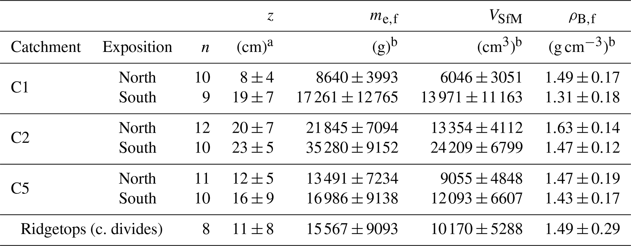
^a Depth below the surface as measured in the field. ^b Uncertainties reported for the excavated mass (field state; m_e,f) and the SfM-MVS photogrammetry-based excavation volume (V_SfM) denote 1σ of the mean value without considering individual measurement errors.

4.2 Field tests

The generally good agreement between SfM-MVS photogrammetry-based and reference volumes is also valid for the BD17 field tests. However, the applied workflows mostly failed to generate accurate and precise reproductions of the volume of the boulder placed into the pits of BD17-P11.1 and BD17-P12.1. This was mainly due to the lack of sufficient image coverage and significant shading, especially of the parts of the boulder located close to the pit ground. These areas were neglected while taking pictures from different angles as they were mostly concealed by the corners of the pit. A stronger variation in shooting distances and angles probably would have improved the results (Mosbrucker et al., 2017, and references therein). Therefore, the imaging strategy during the AT17–18 fieldwork included close-ups of hidden or shaded areas within the respective pits from different angles.

The consistency of values for V_SfM at site BD17-P11 can be regarded as an indication that SfM-MVS photogrammetry reproduced the “true” volume of the pit more accurately than V_PU. This finding might be to a certain extent explained by the way V_PU was derived. The casts of the pits BD17-P11 and BD17-P12 were too large to fit into standard 51 L barrels which were used to submerge the casts into water. As a consequence, they were cut into 13 (BD17-P11) and 12 (BD17-P12) parts, which were then submerged one by one (thereby increasing the measurement error). Although we cut the casts carefully, we could not avoid ripping off a high quantity of small globules from the polystyrene blocks that made up most of the inside filling of the casts. This loss in volume could have contributed to the large difference between the photogrammetry-based volumes and the volumes of the casts for site BD17-P11, although the volume of the cast of BD17-P12 matches the SfM-MVS photogrammetry-based volumes quite well. However, an underestimation of the pit volume of site BD17-P11 by V_PU is further supported if the final photogrammetry-based densities of sites BD17-P01, BD17-P06 and BD17-P11 are compared. All three pits were dug into the same gravel layer within a radius of <20 m. Accordingly, the field-state bulk densities are very similar (about 2.08 to 2.14 g cm⁻³ when the performance-workflow-based volumes are considered; Table 4). These values are further in accordance with the reference densities of BD17-P01 and BD17-P06 (∼2.12 g cm⁻³); only for the reference ρ_B,f of BD17-P11 is a value of 2.34±0.05 g cm⁻³ obtained.

The significant difference between the SfM-MVS photogrammetry-based densities and the densities calculated from the soil sample rings at site BD17-P11 is not surprising as the latter method is not suited to sample such coarse-grained and poorly sorted material (e.g. McLintock, 1959; Muller and Hamilton, 1992). Especially centimetre-sized clasts cause problems recovering all sample material properly. Thus, material intake during the sampling into the soil sample rings is insufficient, and the mass of the sample is underestimated. Furthermore, a continuous sampling from the top to the bottom of the pit's walls was impeded by loose gravel and sand. The high scatter of soil sample ring density data derived from the BD17-P11 site reflects a strong inhomogeneity of the regolith profile, where a ∼8 cm thick loess layer covered gravel layers and a ∼7 cm thick sand layer (see Supplement). The analysis of inhomogeneous soils has been shown to be difficult in terms of accurately measuring bulk densities elsewhere (e.g. Brahim et al., 2012; Manrique and Jones, 1991). This was, however, not the case at sites BD17-P12 and BD17-P13, where the samples were taken from homogenous loess layers. It is likely that compaction, predominantly due to mining traffic and a greater depth below the surface (Manrique and Jones, 1991), caused higher bulk densities at site BD17-P12, which was located on an access ramp. A comparison of the PU foam cast of the cavity dug at site BD17-P13 with the SfM-MVS photogrammetry-based model revealed that the PU foam cast did not include a void at the right outer rim of the cavity. From the picture documentation we realised that this area and the lower rim of the cavity were accidentally cut from the PU cast when the latter was removed from the cavity after hardening, a problem already described by Brye et al. (2004). The cutting was necessary because a wooden board used to prevent the foam from expanding outside the cavity did not completely fit the cavity. As a consequence, the foam did ooze between the rim of the board and the rim of the cavity. However, removing these areas also from the DSLM–performance workflow model yields a volume of 4239±70 cm³ and a field bulk density of 1.52±0.03 g cm⁻³, which is in good agreement with the reference value of 1.54±0.03 g cm⁻³. Vice versa, the (original) SfM-MVS photogrammetry-based densities also match the sample ring-based reference densities. Thus, we conclude that the SfM-MVS photogrammetry-based model of BD17-P13 is more accurate than the PU-foam-based reference value obtained for ρ_B,f, underlining the applicability of the method tested in this study in the field even for sites featuring badly illuminated surfaces (the top of the cavity was heavily shaded; see Supplement). Taken together with the results obtained from the tests performed using the artificial pit in a tilted position (Sect. 3.1), this implies that the method tested here can also be used to estimate densities along sediment depth profiles, where the inherited nuclide concentration, the surface erosion rate and/or the surface age can be derived from TCN depth sampling (e.g. Braucher et al., 2009). For this kind of analysis, the derivation of sediment densities can be complex (for examples see Brye et al., 2004; Rodríguez-Rodríguez et al., 2020), but the (time-integrated) sediment density accuracy and precision can largely affect the overall results (e.g. Braucher et al., 2009; Hidy et al., 2010; Rodés et al., 2011).

As argued for the tests performed on the artificial pit (Sect. 4.1), scaling issues are most likely the main cause of slightly less accurate and precise results obtained from the freeware workflow. The results also further indicate that using imagery data taken with the smartphone camera in JPEG format yields volume reconstructions of similar accuracy to those that are DSLM-based. Thus, there is no need to carry expensive camera equipment in the field if a smartphone is carried that has a camera with comparable hardware properties to the one used in the tests of this study.

In contrast to the tests conducted using the artificial pit, the performance workflow required less time to reconstruct a watertight model (see Table B1). Although the non-automated time fraction of the processing is larger than for the freeware workflow, it is more convenient due to the ability to perform batch processing. Furthermore, the non-automated processing in the performance workflow can potentially be significantly reduced, at the expense of accuracy and precision (Sect. 4.1).

Finally, when compared to the broad range of established methods to determine soil bulk densities, the SfM-MVS photogrammetry-based method as tested in this study regularly yields results of comparable precision and accuracy. Values for measurement precision and/or accuracy as found in the literature are generally about 5 to 15 % of the mean bulk density for the clod, core and non-photogrammetry excavation methods in uniform substrates (Casanova et al., 2016; Coelho, 1974; Grossman and Reinsch, 2002, and references therein; Muller and Hamilton, 1992; Timm et al., 2005). This holds also for some indirect measurement techniques, such as the TDR method (Liu et al., 2008) and nuclear radiation methods (Timm et al., 2005). In contrast to that, soil bulk densities of gravelly soils derived from uncalibrated pedotransfer functions have been shown to be less accurate (Casanova et al., 2016).

4.3 Aspect-related density contrasts in the Altos de Talinay

The results obtained from the stepwise volume derivation at sites AT17-001, AT17-028, and AT17-029 as well as the comparison of densities of close-by dug pits (AT17-032, AT17-032TS, AT18-102(1) and AT18-102(2)) confirm the high precision and accuracy of the SfM-MVS photogrammetry-based soil field bulk densities. In order to scale local TCN production rates for bedrock and/or saprolite covered by soil, ρ_B,f seems to be sufficient in the study area, as values for ρ_B,d mostly do not differ significantly from the field state. Given the assumption that the aliquot sample sufficiently mirrors the physical properties of the entire excavation, the inference of V_a,r is the most delicate step to approximate ρ_d. The comparably small standard deviation (0.11 g cm⁻³) from ρ_BR measurements indicates that, despite some heterogeneities present in the bedrock lithology, it is reasonable to use ρ_BR to approximate ρ_d. V_a,r could also be measured directly, but this can result in high relative measurement uncertainties in soils with low contents of the >2 mm fraction if the aliquot sample size is too small (e.g. Soil Survey Staff, 2014; Vincent and Chadwick, 1994). If no reliable estimation of ρ_BR can be made, a possible workaround could be to sample a certain amount of the >2 mm fraction and measure its volume in the laboratory. Vincent and Chadwick (1994) have shown that a representative sample mass to reflect the particle size distribution of a gravelly soil is on the order of ∼10 kg, which would then have to be sieved in the field to retain the >2 mm fraction. However, this implies that at least one additional sieve and the aliquot material would have to be carried along (e.g. 3 kg of gravel from a soil containing 30 % gravel by mass).

The tendency towards lower values for ρ_B,f (as well as for ρ_B,d and ρ_d in C1 and C2) and higher values for z on SFSs than on NFSs might be linked to slope exposure with respect to insolation, causing contrasting microclimatic conditions and thus the observed differences in vegetation cover and presumed differences in soil properties (e.g. Bockheim and Hartemink, 2017; Dal Bo et al., 2019; Gutiérrez-Jurado and Vivoni, 2013b; Jenny, 1994; Pelletier and Swetnam, 2017). We found that the aspect-related contrasts in measured densities are especially pronounced close to the thalwegs. This finding could be related to the steeper slopes, relief-induced increased soil moisture and a greater shielding from solar radiation in this zone, enhancing the differences in microclimatic conditions, vegetation contrasts and associated weathering and erosion processes (Bernhard et al., 2018; Gutiérrez-Jurado and Vivoni, 2013b; Jenny, 1994; Oeser et al., 2018; Figs. 9 and 10). This assumption could also explain the less pronounced contrasts along the transect in catchment C5, where erosional processes have widened the valley more than at the transects of C1 and C2. We further note that the mean value for ρ_B,f on the SFS of C5 is affected by the fact that we could dig only one pit at the lower portion of the slope due to a general inaccessibility and a great abundance of cobbles and boulders (slope debris) in this area.

The mean differences in bulk densities between NFSs and SFSs are pronounced but not significant, supporting the results of recent studies which did not find significant differences in most present-day physical and chemical properties of regolith on NFSs and SFSs in the Coastal Cordillera of northern Chile (Bernhard et al., 2018; Oeser et al., 2018). Measured soil bulk densities and/or soil depths derived from study sites in the semi-arid natural reserve of Santa Gracia, located ∼120 km NNE of our study area, are very similar to those derived in this study (Bernhard et al., 2018; Dal Bo et al., 2019; Oeser et al., 2018; Owen et al., 2011).

Regarding the quality and expenditure of time to derive the final watertight meshes, we did not find significant differences between the two DSLM cameras used. As 30 or fewer pictures in total was sufficient to generate watertight models accurately reflecting the original pit, both semi-automated marker placement/scaling and automated computing time were likely unnecessarily increased at many sites (e.g. Eltner et al., 2016). The main driver of time consumption for the automatic process steps is the number of pictures that have been taken. Although the computer hardware in use was less powerful than that used during the testing phase, computing times are comparable, emphasising that consumer-grade computer hardware is also sufficient to generate watertight meshes in reasonable time. However, the placement of markers required the bulk of the expenditure of time. Besides the marker/scaling issues discussed for the tests performed on the artificial pit (the marked photographic reference scales were not used during the BD17 field tests and the field campaign), the alignment of the pre-dug and the pit surfaces were time-consuming. To overcome this problem, we suggest using at least four screw-and-washer assemblies per setting, which can serve as fixed reference points in both the pre-dug and the pit surfaces. Screw-and-washer assemblies are lightweight and do not add a significant amount of baggage to the total baggage to be carried into the field.

5 Conclusion

For several fields of research, including the inferences of process rates and ages based on the quantification of concentrations from TCNs, accurate knowledge of soil bulk densities can be of great importance. We have tested SfM-MVS photogrammetry-based workflows which are suited for non-expert applicants (in photography, the SfM-MVS photogrammetry technique and programming) to measure soil bulk densities that yield results of high accuracy and precision (generally >95 %) if a proper imaging strategy is applied and a consumer-grade camera is used. Furthermore, watertight models of the excavation from an imagery dataset can be derived without any extra costs if an up-to-date computer is available. The method is especially suited for fieldwork teams that work in remote areas and whose capability to carry tools and/or samples is limited by backpack space and work force. If the sampling for TCNs requires the excavation of soil, the overall sampling procedure is not significantly prolonged by weighting the excavated material and taking pictures. If deeper knowledge on soil properties is required or values for ρ_B,d and ρ_d should be inferred, an aliquot-size sampling of the soil can yield reasonable approximations in gravelly soils. By applying the method in a study area in the Coastal Cordillera of northern central Chile, we found field-state bulk density values to generally reflect slope aspect, although the differences between NFSs and SFSs are insignificant. However, significant differences are detectable along diffusively eroding slope noses within a few tens of metres. This indicates that the determination of a single slope-wide density value for cosmogenic nuclide analysis would be insufficient to accurately characterise surface process rates along the slope.

Appendix A: List of mathematical symbols

fd	Conversion factor to approximate the dry mass of an excavation
fr,d	Conversion factor to approximate the mass of the >2 mm fraction of an oven-dried excavation
fr,V	Conversion factor to approximate the volume of the >2 mm fraction of an excavation
ma,f	Mass of an aliquot sample in field state (in g)
ma,d	Mass of an oven-dried aliquot sample (in g)
ma,r	Mass of the fraction >2 mm in an aliquot sample (in g)
me,d	Total oven-dried mass of an excavation (in g)
me,f	Total mass of an excavation in field state (in g)
P(z)	TCN production rate for a given depth (in atoms g−1 yr−1)
P0	TCN production rate at the surface (in atoms g−1 yr−1)
V	Volume (in cm3)
Va,r	Volume of the fraction >2 mm in an aliquot sample (in cm3)
Vb,SfM	SfM-MVS photogrammetry-based volume of the boulder used during the field tests
	in BD17-P11.1 and BD17-P12.1 (in cm3)
Vb,ref	Reference volume of the boulder used during the field tests in BD17-P11.1 and BD17-P12.1 (in cm3)
VSfM	SfM-MVS photogrammetry-based volume of a soil pit (in cm3)
VPU	Reference volume of a soil pit based on PU foam casts (in cm3)
z	Soil depth (in cm)
Λ	Attenuation path length of cosmic rays (in g cm−2)
ρ	Density (in g cm−2)
ρB	Soil bulk density (in g cm−2)
ρB,d	Dry soil bulk density (in g cm−2)
ρB,f	Field-state soil bulk density (in g cm−2)
ρBR	Bedrock density (in g cm−2)
ρd	Dry soil density (in g cm−2)
${\mathit{\rho }}_{{\mathrm{H}}_{\mathrm{2}}\mathrm{O}}$	Density of water (in g cm−2)

Appendix B: Tables

Table B1 Time required to derive watertight models of the soil pits for both workflows and all cameras applied.

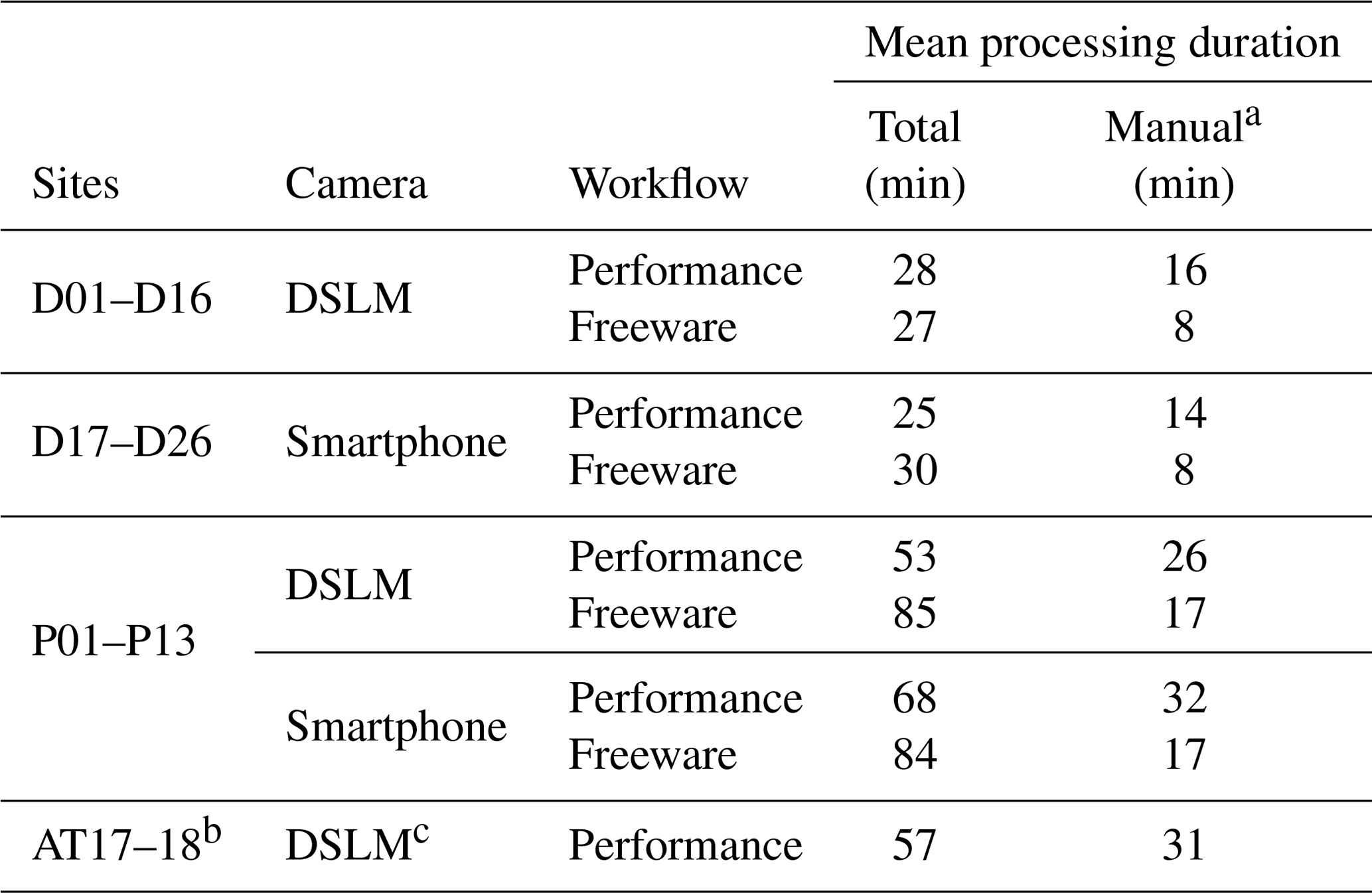
^a Includes the semi-automated referencing via placing markers in Agisoft Metashape. ^b Computing performed on a consumer-grade computer (years 2019/2020). ^c Two different camera models used (both with 16 MP resolution).

Table B2 Comparison of field-state (ρ_B,f) and dry bulk densities (ρ_B,d) for the different workflows and cameras tested.

^a Field-state excavation mass. ^b Oven-dried excavation mass. ^c Uncertainties include the 1σ uncertainty in volume as obtained from the tests performed on the artificial pit and the accuracy of the balance used.

Table B3 Samples from sample rings taken at sites BD17-P11, BD17-P12 and BD17-P13.

^a Depth below the surface. ^b Field-state excavation mass. ^c Oven-dried excavation mass. ^d Field-state bulk density. ^e Dry bulk density. ^f Samples taken a few centimetres above, to the right and to the left of the cavity.