the Creative Commons Attribution 4.0 License.
the Creative Commons Attribution 4.0 License.
 | 26 Aug 2021
Beyond 2D landslide inventories and their rollover: synoptic 3D inventories and volume from repeat lidar data
Thomas G. Bernard
Dimitri Lague
Philippe Steer
Efficient and robust landslide mapping and volume estimation is essential to rapidly infer landslide spatial distribution, to quantify the role of triggering events on landscape changes, and to assess direct and secondary landslide-related geomorphic hazards. Many efforts have been made to develop landslide mapping methods, based on 2D satellite or aerial images, and to constrain the empirical volume–area (V–A) relationship which, in turn, would allow for the provision of indirect estimates of landslide volume. Despite these efforts, major issues remain, including the uncertainty in the V–A scaling, landslide amalgamation and the underdetection of landslides. To address these issues, we propose a new semiautomatic 3D point cloud differencing method to detect geomorphic changes, filter out false landslide detections due to lidar elevation errors, obtain robust landslide inventories with an uncertainty metric, and directly measure the volume and geometric properties of landslides. This method is based on the multiscale model-to-model cloud comparison (M3C2) algorithm and was applied to a multitemporal airborne lidar dataset of the Kaikōura region, New Zealand, following the Mw 7.8 earthquake of 14 November 2016.
In a 5 km2 area, the 3D point cloud differencing method detects 1118 potential sources. Manual labeling of 739 potential sources shows the prevalence of false detections in forest-free areas (24.4 %), due to spatially correlated elevation errors, and in forested areas (80 %), related to ground classification errors in the pre-earthquake (pre-EQ) dataset. Combining the distance to the closest deposit and signal-to-noise ratio metrics, the filtering step of our workflow reduces the prevalence of false source detections to below 1 % in terms of total area and volume of the labeled inventory. The final predicted inventory contains 433 landslide sources and 399 deposits with a lower limit of detection size of 20 m2 and a total volume of 724 297 ± 141 087 m3 for sources and 954 029 ± 159 188 m3 for deposits. Geometric properties of the 3D source inventory, including the V–A relationship, are consistent with previous results, except for the lack of the classically observed rollover of the distribution of source area. A manually mapped 2D inventory from aerial image comparison has a better lower limit of detection (6 m2) but only identifies 258 landslide scars, exhibits a rollover in the distribution of source area of around 20 m2, and underestimates the total area and volume of 3D-detected sources by 72 % and 58 %, respectively. Detection and delimitation errors in the 2D inventory occur in areas with limited texture change (bare-rock surfaces, forests) and at the transition between sources and deposits that the 3D method accurately captures. Large rotational/translational landslides and retrogressive scars can be detected using the 3D method irrespective of area's vegetation cover, but they are missed in the 2D inventory owing to the dominant vertical topographic change. The 3D inventory misses shallow (< 0.4 m depth) landslides detected using the 2D method, corresponding to 10 % of the total area and 2 % of the total volume of the 3D inventory. Our data show a systematic size-dependent underdetection in the 2D inventory below 200 m2 that may explain all or part of the rollover observed in the 2D landslide source area distribution. While the 3D segmentation of complex clustered landslide sources remains challenging, we demonstrate that 3D point cloud differencing offers a greater detection sensitivity to small changes than a classical difference of digital elevation models (DEMs). Our results underline the vast potential of 3D-derived inventories to exhaustively and objectively quantify the impact of extreme events on topographic change in regions prone to landsliding, to detect a variety of hillslope mass movements that cannot be captured by 2D landslide mapping, and to explore the scaling properties of landslides in new ways.
- Article
(27649 KB) - Full-text XML
-
Supplement
(1924 KB) - BibTeX
- EndNote


In mountainous areas, extreme events such as large earthquakes and typhoons can trigger important topographic changes through landsliding. Landslides are a key agent of hillslope and landscape erosion (Keefer, 1994; Malamud et al., 2004) and represent a significant hazard for local populations (e.g., Pollock and Wartman, 2020). Efficient, rapid and exhaustive mapping of landslides is required to robustly infer their spatial distribution, their total volume and the induced landscape changes (Guzzetti et al., 2012). Such information is crucial to understand the role of triggering events on landscape evolution and to manage direct and secondary landslide-related hazards. For instance, it is essential to evaluate the total volume produced by landsliding if earthquakes tend to build or destroy topography (e.g., Marc et al., 2016; Parker et al., 2011) in order to quantify the contribution of extreme events to long-term denudation (Marc et al., 2019) or to predict hydro-sedimentary hazards such as river avulsion related to the downstream transport of landslide debris (Croissant et al., 2017). Following a triggering event, total landslide volume at the regional scale is classically determined in two steps. The first is individual landslide mapping using 2D satellite or aerial images (e.g., Behling et al., 2014; Fan et al., 2019; Guzzetti et al., 2012; Li et al., 2014; Malamud et al., 2004; Martha et al., 2010; Massey et al., 2018; Parker et al., 2011), and the second is indirect volume estimation using a volume–area relationship (e.g., Larsen et al., 2010; Simonett, 1967):
where V and A are the volume and area of individual landslides, respectively; α is a prefactor; and γ is a scaling exponent usually ranging between 1.1 and 1.6 (e.g., Larsen et al., 2010; Massey et al., 2020; Pollock and Wartman, 2020).
A first source of error comes from the uncertainty in the values of α and γ, which tend to be site-specific and potentially process-specific (e.g., shallow versus bedrock landsliding). This uncertainty could lead to an order of magnitude difference in the total estimated volume given the nonlinearity of Eq. (1) (Larsen et al., 2010). Two other sources of error arise from (1) the inherent detectability of individual landslides and (2) the ability to accurately measure the distribution of landslide areas due to landslide amalgamation and underdetection of landslides. Landslide amalgamation can produce up to a 200 % error in the total volume estimation (Li et al., 2014; Marc and Hovius, 2015) and occurs because of landslide spatial clustering or incorrect mapping due, for instance, to automatic processing. Indeed, automatic landslide mapping (Behling et al., 2014; Marc et al., 2019; Martha et al., 2010; Pradhan et al., 2016) relies on the difference in texture, color and spectral properties such as the NDVI (normalized difference vegetation index) between pre- and post-landslide images, assuming that landslides lead to vegetation removal or significant texture change. During this process, difficulties in automatic segmentation of landslide sources can result in the amalgamation of individual landslide areas; this propagates into a much larger errors in volume owing to the nonlinearity of Eq. (1). Manual mapping and automatic algorithms based on geometrical and topographical inconsistencies can reduce the amalgamation effect on landslide volume estimation (Marc and Hovius, 2015), but it remains a source of error due to the inherent spatial clustering of landslides and the overlapping of landslide deposits and sources (Tanyaş et al., 2019).
Underdetection of landslides can occur because the spectral signature of images is not altered enough by a new failure; hence, the algorithm or person identifying the landslides cannot detect the event. Notably, underdetection of small landslides is one hypothesis put forward to explain the divergence of small landslides from the power-law frequency–area distribution observed for medium to large landslides (e.g., Bellugi et al., 2021; Stark and Hovius, 2001; Tanyaş et al., 2019). A rollover point below which frequencies decrease for smaller landslides is observed, and varies between 40 and 4000 m2 for different inventories (Tanyaş et al., 2019). Beyond the underdetection of small landslides, other explanations for the occurrence of a rollover have been put forward, notably the transition from a friction-dominated mode of rupture for large landslides to a cohesion-dominated mode for small landslides (e.g., Jeandet et al., 2019; Tanyaş et al., 2019; and references therein). Underdetection can be particularly common in areas with thin soils and sparse or missing vegetation (Barlow et al., 2015; Behling et al., 2014; Brardinoni and Church, 2004; Miller and Burnett, 2007). It can be further complicated when using different image sources with different spatial resolutions, spectral resolutions, projected shadows and, consequently, varying abilities to detect surface change. However, the level of landslide underdetection in a given inventory remains generally largely unknown. Therefore, a new method to detect landslides in areas with sparse or a complete lack of vegetation are critically needed. To deal with poorly vegetated areas, Behling et al. (2014, 2016) developed a method using temporal NDVI trajectories that describes the temporal footprints of vegetation changes but cannot fully address complex cases when texture is not significantly changing such as bedrock landsliding on bare-rock hillslopes.
Addressing these three sources of uncertainty – volume–area scaling uncertainty, landslide amalgamation and the underdetection of landslides – is necessary. In the last decade, the increasing availability of multitemporal high-resolution 3D point cloud data and digital elevation models (DEMs), based on aerial or satellite photogrammetry and light detection and ranging (lidar), has opened the possibility to better quantify surface change and displacements (e.g., Bull et al., 2010; Mouyen et al., 2020; Okyay et al., 2019; Passalacqua et al., 2015; Ventura et al., 2011).
The most commonly used technique is the difference of DEM (DoD) which computes the vertical elevation differences between two DEMs from different times (Corsini et al., 2009; Giordan et al., 2013; Mora et al., 2018; Wheaton et al., 2010). Even though this method is fast and works properly on horizontal surfaces, vertical differences can be prone to strong errors when used to quantify changes on vertical or very steep surfaces where landsliding typically occurs (e.g., Lague et al., 2013). In contrast, the multiscale model-to-model cloud comparison (M3C2) algorithm implemented by Lague et al. (2013) considers a direct 3D point cloud comparison. This algorithm has three main advantages over DoD: (i) it operates directly on 3D point clouds, avoiding a phase of DEM creation that is conducive to a loss of resolution imposed by the cell size and potential data interpolation; (ii) it computes 3D distances along the normal direction of the topographic surface, allowing better capture of subtle changes on steep surfaces; and (iii) it computes a spatially variable confidence interval that accounts for surface roughness, point density and uncertainties in data registration. Applicable to any type of 3D data to measure the orthogonal distance between two point clouds, this approach has generally been used for terrestrial lidar and UAV (unoccupied aerial vehicle) photogrammetry over sub-kilometer scales. In the context of landsliding, it has been used to infer the displacement and volume of individual landslides, using point clouds obtained by UAV photogrammetry (e.g., Esposito et al., 2017; Stumpf et al., 2015), as well as for rockfall studies (Benjamin et al., 2020; Williams et al., 2018) and sediment tracking in post-wildfire conditions (DiBiase and Lamb, 2020). To our knowledge, systematic detection and segmentation of hundreds of landslides from 3D point clouds have not yet been attempted.
Here, we produce an inventory map of landslide topographic changes using a semiautomatic 3D point cloud differencing (3D-PcD) method based on M3C2 and applied to multitemporal airborne lidar data. We use the generic term “landslide” to define the spatially coherent changes detected by our method on hillslopes that result in at least several decimeters of negative topographic change associated with a downstream positive topographic change. Patches of negative (positive) topographic change are called sources (deposits) and correspond to erosion (sedimentation) for landslides producing debris or to subsidence (accumulation) for landslides involving the movement of largely intact hillslope material. Therefore, this definition includes all types of mass-wasting processes involving the downward or outward movement of soil, rocks and debris under the influence of gravity, occurring on discrete boundaries and initially taking place without the aid of water as a transportational agent (Crozier, 1999). An objective of this work is to provide a first evaluation of the type of landslides produced during an earthquake that 3D point cloud differencing can detect.
Our workflow was designed to be as automated as possible in order to be applied to very large multitemporal 3D datasets in the future. As any topographic data will contain elevation errors (Anderson, 2019; Joerg et al., 2012; Passalacqua et al., 2015) that may result in false detections of sources and deposits, our workflow combines two steps to filter them out: we first isolate patches of significant topographic change using the statistical model accounting for point cloud roughness, density and registration error defined in the M3C2 algorithm (Lague et al., 2013), and we then use patch-based metrics to detect the remaining false detections. The workflow efficiency is tested against a set of sources manually labeled as actual landslides or false detections. We apply our method to a complex topography located near Kaikōura, New Zealand, where a Mw 7.8 earthquake triggered nearly 30 000 landslides over a 10 000 km2 area in 2016 (Massey et al., 2020). We choose a 5 km2 area characterized by a high landslide spatial density along the Conway segment of the Hope Fault, which was inactive during the earthquake, where pre- and post-earthquake lidar and aerial images were available (Fig. 1). This area has a variety of vegetation cover (e.g., dense evergreen forest, sparse or small shrubs and grass, bare bedrock) and typically represents a challenge for conventional 2D landslide mapping. We apply our workflow to obtain a 3D landslide inventory that is compared to a traditional manually mapped inventory of landslide scars based on aerial image comparison, hereafter called the 2D inventory. We illustrate the benefits of working directly on 3D data to generate landslide source and deposit inventories, and we discuss the methodological advantages of operating directly on point clouds with M3C2 compared with DoD, in terms of detection accuracy and error for total landslide volume.
The paper is organized as follows: first, the lidar dataset is presented, followed by a detailed description of the 3D-PcD method; second, results of the geomorphic change detection and identification of individual landslides in the studied area are presented. The remaining part of the paper focuses only on landslide sources. First, we evaluate the prevalence of false detections and define optimal filtering parameters to be used to limit their occurrence. Second, the comparison with conventional 2D landslide mapping is presented. Third, the statistical properties of the 3D and 2D landslide source inventories are investigated in terms of area and volume. Finally, current limitations of the method are discussed as well as knowledge gained on the importance of landslide underdetection on the coseismic landslide inventory budget, the variety of landsliding processes that can be detected by our workflow and landslide source geometry statistics.
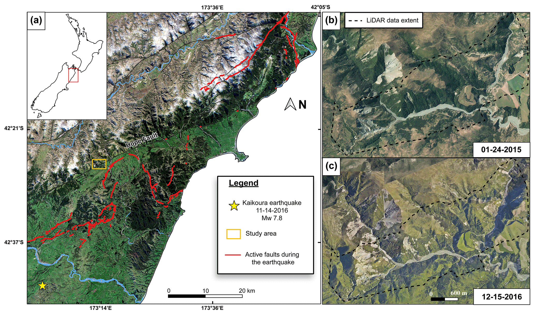
Figure 1Maps of the regional context and location of the study area: (a) regional map of Kaikōura with the location of the 2016 Mw 7.8 earthquake, associated active faults and the study area; orthoimages focused on the study area dated before (b) and after (c) the earthquake with the 5 km2 lidar dataset extent used in this paper (all images are available at https://canterburymaps.govt.nz/about/feedback/ (last access: 18 July 2021); Aerial Surveys, 2017).
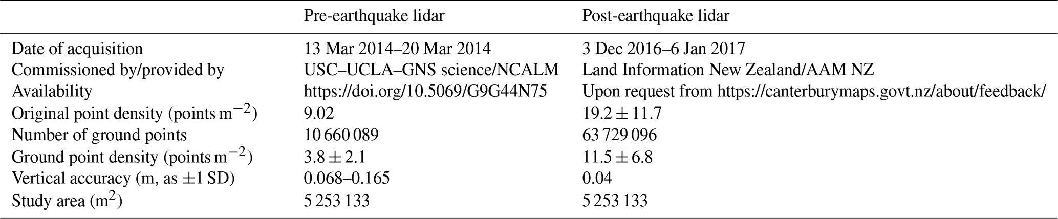
In this study, we compare two 3D point clouds obtained from airborne lidar data collected before and after the 14 November 2016 Kaikōura earthquake (Table 1). Both airborne lidar surveys were carried out during summer. Pre-earthquake (pre-EQ) lidar data were collated over six flights performed from 13 to 20 March 2014 for a resulting ground point density of 3.8 ± 2.1 points m−2. The vertical accuracy of this dataset has been estimated at 0.068–0.165 m as the standard deviation of the difference between the elevation of GPS points located on highways and the nearest-neighbor lidar shot elevation (Dolan, 2014). However, these control points were not in the survey area. Thus, we have weak independent constraints on the vertical accuracy of the pre-EQ lidar in the survey area. The post-earthquake (post-EQ) lidar survey took place soon after the earthquake, from 3 December 2016 to 6 January 2017, for an average ground point density of 11.5 ± 6.8 points m−2. The vertical accuracy of this dataset has been estimated following the same protocol as the pre-earthquake lidar data with a mean of 0.00 m and a standard deviation of 0.04 m (Aerial Surveys, 2017). The difference in acquisition dates represents a period of 2 years and 8 months. For both lidar point clouds, only ground points defined by the data providers are selected. For the pre-EQ lidar, they were classified automatically using the TerraScan software (Dolan, 2014), whereas the post-EQ data were classified using an unspecified algorithm followed by manual validation by the data provider (Aerial Surveys, 2017). Manual quality control shows that ground classification is excellent for the post-EQ data but that some points corresponding to vegetation remain in the pre-EQ data. As the incorrectly classified points are located a few meters above the ground, they can lead to false landslide source detection because they translate into a negative topographic change (i.e., apparent spatially correlated erosion). Thus, we reprocess this dataset to remove as many incorrectly classified points as possible using a method similar to surface-based filtering that removes points or patches of points significantly higher than the locally interpolated ground (e.g., Kraus and Pfeifer, 1998) (details in Sect. S1 in the Supplement). This operation removes 0.3 % of the pre-EQ original point cloud, but our results show that classification errors still remain. We did not attempt to further improve the classification, as these errors are expected to occur in a low-point-density lidar survey of evergreen forested areas and will generate false landslide sources that our workflow should detect and filter out. We note that the classification refinement is not a critical component of our workflow and that other classifications algorithms (Sithole and Vosselman, 2004) could be used to improve or check the quality of the lidar ground points before the application of the workflow.
In addition, orthoimages are used to perform a manual mapping of landslides to compare the detection of landslides from the 3D approach and a more classical approach. The pre-EQ orthoimage was obtained on 24 January 2015 (available at https://data.linz.govt.nz/layer/52602-canterbury-03m-rural-aerial-photos-2014-2015, last access: 20 July 2021), and the post-EQ image was obtained on 15 December 2016. The resolutions of these images are 0.3 and 0.2 m, respectively.
3.1 The 3D point cloud differencing with M3C2 and the distance uncertainty model
The method developed here to detect landslides consists of 3D point cloud differencing between two epochs using the M3C2 algorithm (Lague et al., 2013) available in the CloudCompare software (EDF R&D, 2011). This algorithm estimates orthogonal distances along the surface normal directly on 3D point clouds without the need for surface interpolation or gridding. While M3C2 can be applied on all points, the algorithm can use an accessory point cloud, called core points. In our case, core points constitute a regular grid with constant horizontal spacing generated by the rasterization of one of the two clouds. In the following, all the M3C2 calculations are done in 3D using the raw point clouds, but the results are “stored” on the core points. The use of a regular grid of core points has four advantages: (i) the regular sampling of the results allows the computation of robust statistics of changes, unbiased by spatial variations in point density; (ii) it facilitates the volume calculation and the uncertainty assessment; (iii) it can be directly reused with 2D GIS (geographic information system) as a raster (rather than a non-regular point cloud); and (iv) it speeds up calculations, although in the proposed workflow, computation time is not an issue, and the calculations can be done on a regular laptop.
The first step of M3C2 consists of computing a 3D surface normal for each core point at a scale D (called the normal scale) by fitting a plane to the core points located within a radius of size . Once the normal vectors are defined, the local distance between the two clouds is computed for each core point as the distance along the normal vector of the arithmetic mean positions of the two point clouds at a scale d (projection scale). This is done by defining a cylinder of radius , oriented along the normal with a maximum length pmax. Distances are not computed if no intercept is found in the second point cloud (that is, in areas where the two point clouds do not overlap) or if one cloud has missing ground data (e.g., below dense forest cover). pmax must be chosen to be larger than the largest topographic change to be measured. Thus, pmax can be as large as several tens of meters in landslide inventories. This poses a potential issue in highly curved features of the landscape such as narrow ridges or gorges with steep flanks where the cylinder can intercept the same point cloud twice, resulting in an incorrect distance calculation. A preliminary analysis showed that this resulted in about 1 % of false landslide detections. Thus, we have modified the M3C2 algorithm to avoid the double-intercept issue. A new iterative procedure progressively increases the depth of the cylinder up to pmax, by intervals of 1 m for each core point, and checks for the stability of the measured distance: if the distance is stable for two successive iterations, it is considered as the final M3C2 distance for this core point. This modification solved the double-intercept issue.
M3C2 has the option of computing the distance vertically, which bypasses the normal calculation, and we use this option several times in the workflow. We use the abbreviation “vertical-M3C2” in these cases and “3D-M3C2” otherwise. M3C2 also provides the uncertainty in the computed distance at the 95 % confidence level based on local roughness, point density and registration error as follows:
where LoD95 % is the level of detection; t is the two-tailed t statistics with a confidence level of 95 % and a degree of freedom DF (Borradaile, 2003); σ1(d) and σ2(d) are the standard deviation of distances of each cloud, at scale d,measured along the normal direction; n1 and n2 are the number of points in each cloud at that scale; and reg is the co-registration error between the two epochs. When the M3C2 distance is larger than the LoD95 %, the topographic change is considered statistically significant. In Eq. (2), the first two terms assume that σ1(d) and σ2(d) empirically characterize two uncorrelated random errors depending on the topographic surface roughness and the survey precision. On perfectly flat surfaces, σ(d) is minimal and characterizes the instrument precision; however, on rough surfaces, σ(d) will increase above this value and becomes the dominant source of uncertainty (Lague et al., 2013). As we consider these sources of uncertainty as uncorrelated random errors, increasing the number of samples n1 and n2 reduces the LoD95 %. The original M3C2 algorithm uses a value of t equal to 1.96, the asymptotic value of the two-tailed t statistics when F is infinite, and the LoD95 % is only computed if n1 > 4 and n2 > 4. As will be shown later, the low point density of the pre-EQ data in forested areas resulted in values of n1 varying between 5 and 15, in which case t(F(n1,n2)) is significantly larger than 1.96. For instance, when 5, F= 4 and t= 2.776. To avoid underpredicting LoD95 % in low-point-density areas, we choose to apply the strict two-tailed t statistics rather than the simplification used in the CloudCompare implementation of M3C2. As point density and surface roughness are spatially variable, LoD95 % is also spatially variable. For instance, on forested steep hillslopes, points located under the canopy, with a lower point density, or vegetation points that are incorrectly classified as ground and create locally high roughness, result into a higher LoD95 % and, therefore, require a larger topographic change to be detected as significant change.
The co-registration error reg in Eq. (2) is treated as a systematic spatially uniform error encompassing all the errors that are not uncorrelated random errors. However, this is a simplification, as elevation errors related to intra-flight-line time-dependent attitude and position uncertainties combine with intra-survey registration errors of flight lines and the inter-survey rigid registration error to make reg theoretically spatially variable (Joerg et al., 2012; Passalacqua et al., 2015). These error sources may create apparent low-amplitude and variable-wavelength topographic change that could be mistakenly considered as a significant change resembling a landslide source or deposit if reg is not high enough. Predicting the spatial pattern of registration error can be done in two ways. The first method involves using a spatially explicit direct error propagation model that accounts for all elevation errors in the lidar survey (e.g., Joerg et al., 2012). This approach is complex and requires detailed information on the survey, including the trajectory file with the position and attitude uncertainties. This file is rarely available in data repositories and was not available for the pre-EQ or post-EQ datasets. The second approach involves studying patterns of topographic change on flat, stable and near-horizontal surfaces (e.g., Anderson, 2019) to derive amplitude and spatial correlation characteristics of the registration error. The stable area must not have changed between the survey and must be much larger than the expected spatial correlation scale. It also has to be as flat as possible to limit the effect of surface roughness, which (being sampled differently between each survey) may obscure the correct estimate of registration errors. This approach only captures the spatial patterns of registration error in a statistical sense (using, for instance, a semi-variogram; Anderson, 2019) and, thus, corresponds to a spatially uniform reg. This approach cannot be applied in our case, as we lack extensive, flat, smooth and stable areas such as human infrastructure (e.g., roads, parking lots). Hence, we assume that reg is uniform and isotropic.
A critical aspect of the workflow is to choose the lowest reg possible that does not result in too many false detections. A first estimate of reg can be evaluated from the vertical accuracies provided with the lidar datasets, assuming that no systematic bias remains after the registration process (Table 1). If we assume that the two vertical elevation errors are uncorrelated, reg is the square root of the sum of the square accuracies and varies between 0.08 and 0.17 m. If we assume that the two accuracies are perfectly correlated, which is a worst-case scenario, reg is simply the sum of the two accuracies and would vary between 0.12 and 0.21 m. In both cases, it is largely set by the accuracy of the pre-EQ survey (Table 1). As no GCPs (ground control points) used to evaluate the lidar survey accuracy are applied in our study area (which will generally be the case in steep mountain areas where landslide inventory creation will be meaningful), we propose not relying on the stated lidar accuracies. Instead, we define reg empirically as the standard deviation of 3D-M3C2 distances calculated on stable areas that are manually delimited (see Sect. 3.4.1). However, to better account for the potential poor quality of intra-survey registration error, we define reg as the maximum of the intra-survey and inter-survey registration errors. The intra-survey reg is computed on the overlapping parts of flight line (see Sect. 3.4.1). Finally, the M3C2 definition of the LoD95 % makes the conservative choice of adding reg to the combined standard error related to point cloud roughness, rather than taking the square root of the sum of squares standard error and squared registration error (e.g., Anderson, 2019; Joerg et al., 2012). This arbitrary choice, similar to Lague et al. (2013), ensures that the frequency of false detection of statistically significant change is below 5 %, at the expense of a reduced capacity to detect real small topographic changes close to the LoD95 %.
3.2 The same surface different sampling test
Following the approach proposed in Lague et al. (2013), we employ a test based on using different sampling of the same natural surface to tune parameters of the workflow. To this end, we create two randomly subsampled versions of the post-EQ lidar data (which has the largest point density) with an average point density equal to the pre-EQ data. The resulting point clouds correspond exactly to the same surface (i.e., reg = 0), with roughness characteristics typical of the studied area, but with different point sampling. We subsequently refer to this type of approach as a “same surface different sampling” (SSDS) test.
3.3 Parameter selection and 3D point cloud differencing performance
In this section, we explain how to select the appropriate normal scale D and projection scale d to detect landslides using M3C2. The normal scale D should be large enough to encompass enough points for a robust calculation and to smooth out small-scale point cloud roughness that results in normal orientation flickering and overestimation of the distance between surfaces (Lague et al., 2013). However, D should also be small enough to track the large-scale variations in hillslope geometry. By studying roughness properties of various natural surfaces, Lague et al. (2013) proposed that the ratio of the normal scale and the surface roughness, measured at the same scale, should be larger than about 25. Thus, we set D as the minimum scale for which a majority of core points verify this condition. As roughness is a scale- and point-density-dependent measure, we explore a range for D from 2 m to 15 m for the pre-EQ dataset, which has the lowest point density (Fig. 2a). We found that D∼10 m represents a threshold scale below which the number of core points verifying this condition significantly drops.
The projection scale d should be chosen such that it is large enough to compute robust statistics using enough points but small enough to avoid spatial smoothing of the distance measurement. Following Lague et al. (2013), M3C2 computes Eq. (2) only if five points are included in the cylinder of radius for each cloud. In our case, the pre-EQ data with the lowest point density will set the value of d. We use an SSDS test, applying M3C2 with D= 10 m and d varying from 1 to 40 m. The results (Fig. 2b) show the following: (i) when it can be computed, the LoD95 % actually predicts no significant change for at least 95 % of the time, indicating that the statistical model behind the uncorrelated random error component of Eq. (2) (Lague et al., 2013) is correct for this dataset; (ii) the fraction of core points for which the LoD95 % can be calculated rapidly increases between d= 1 and 8 m, at which point it reaches 100 %. We chose d= 5 m, as it represents a good balance between the ability to compute LoD95 % on most core points (here, ∼97 %) and the smallest projection scale possible. To be able to generate M3C2 confidence intervals for as many points as possible, in particular on steep slopes below vegetation, we employ a second pass of M3C2 with d= 10 m and using the core points for which no confidence interval was calculated at d= 5 m. We note that d could theoretically be set as a function of the lowest mean point density of the two lidar datasets, res, by res. In our case, the pre-EQ dataset has res = 3.8 points m−2 and would predict d= 1.3 m. However, the presence of vegetation significantly reduces the ground point density in some parts, and the overlapping of flight lines creates localized high point density. Therefore, examining the mean ground point density of the entire dataset gives an incomplete picture of the strong spatial variations in point density. These changes in point density, critical to the correct evaluation of the LoD95 % (Eq. 2), are generally lost when working on a raster of elevation (e.g., DEM).
The spacing of the core point grid should be smaller than half the projection scale d to ensure that all potential points are covered by at least one M3C2 measurement and should be larger than the typical point cloud spacing of the lowest-resolution dataset. Because the ground point density on a steep forested hillslope of the 2014 survey is of the order of 1 points m−2, we set a core point spacing of 1 m.
Finally, the maximum cylinder length pmax was set to 30 m, as it encompassed the maximum change observed in the study area. This is generally obtained by trial and error. Setting pmax to an overly large value increases the computation time significantly.
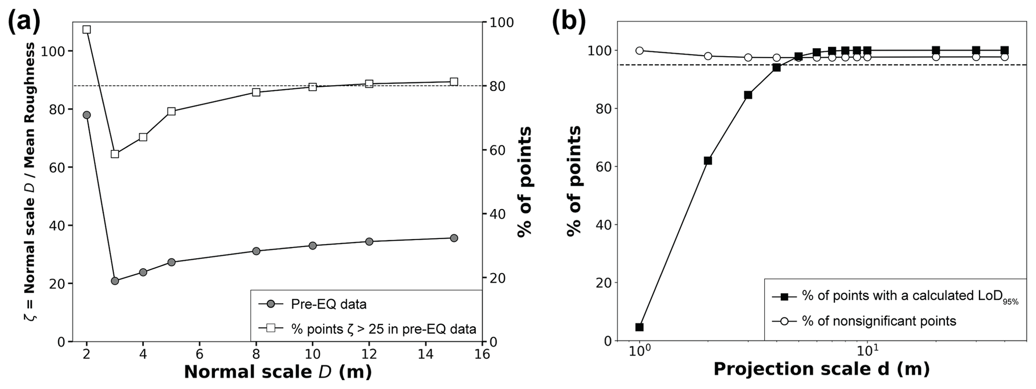
Figure 2Analysis of two main parameters of the M3C2 algorithm: the normal scale D and the projection scale d. Panel (a) shows the ratio between the normal scale and mean roughness for different normal scale values (circles, left y axis), and the fraction of the pre-earthquake core points for which the normal scale is 25 times larger than the local roughness (squares, right y axis). The dashed line highlights the percentage of points with ζ >25 in the pre-EQ data for D= 10 m. Panel (b) shows the percentage of computed points with a confidence interval of 95 % versus the projection scale d. The percentage of nonsignificant points is represented as well as the percentage of points where the level of detection (LoD95 %) was computed (i.e., with at least five points on each point cloud). The dashed line is set to 95 % and highlights the threshold above which the projection scale is large enough to compute the LoD95 % on most of the core points.

Figure 3(a, b, c) Workflow of the 3D point cloud differencing method for landslide detection and volume estimation with schematic representations of the different steps: (a) the 3D measurement step with the shadow zone effect, where the red lines show the normal orientation; (b) the vertical-M3C2 step; (c) segmentation by the connected component. The resulting sources and deposits are individual point clouds illustrated in the figure using different colors.
3.4 The 3D landslide mapping workflow and parameter selection
Our 3D landslide mapping workflow is divided in five main steps (Fig. 3), which are outlined in the following subsections.
3.4.1 Registration of the datasets and the registration error estimate
To detect geomorphic changes and landslides, the two datasets need to be co-registered as closely as possible, and any large-scale tectonic deformation needs to be corrected. The registration error to be used in Eq. (2) must also be estimated.
First, a preliminary quality control is performed to evaluate the intra-survey registration quality of each dataset. This is feasible if the individual flight lines can be isolated using, for instance, the pointID information specific to each line and provided in the LAS file format. The intra-survey registration quality can be investigated with 3D-M3C2 measurements of overlapping flight lines using a 1 m regular grid of core points, from which we define the registration bias and error as the mean and standard deviation of the 3D-M3C2 distances, respectively. The point cloud of the pre-EQ dataset results from 12 flight lines that have overlaps ranging from 60 % to 90 % (Fig. S1 in the Supplement), whereas the post-EQ point cloud corresponds to 5 flight lines with an overlap of 50 %. For each dataset, no significant bias with respect to registration is measured between lines (maximum of 3 cm for the pre-EQ survey and 1 cm for the post-EQ survey; Table S1 in the Supplement), but the registration error ranges from 13 to 20 cm for the pre-EQ survey, and is typically around 6 cm for the post-EQ survey, with one pair of overlapping flight lines having a registration error of 12 cm. Hence, the internal registration quality of the pre-EQ dataset is significantly worse than the post-EQ dataset, a likely consequence of differences in instrument precision and post-processing methods.
Second, the registration between the two surveys must be evaluated and generally improved. As delivered, the lidar datasets have a vertical shift of between 1 and 2 m relative to each other. To correct for this shift, a grid of core points is first created by rasterizing the dataset with the largest point density – here the post-EQ dataset – with a 1 m grid spacing. A vertical-M3C2 calculation is then performed, and the mode of the resulting distribution is used to adjust the two datasets by a vertical shift of 1.36 m. This approach is only valid when the fraction of the surface affected by landsliding is small. A subsequent 3D-M3C2 calculation is performed to obtain a preliminary map of geomorphic change. At this stage, a visual inspection of the pre-EQ and post-EQ orthoimages and of the preliminary 3D-M3C2 distances allows us to determine that there is no significant internal tectonic displacement. We then manually define areas deemed stable, 25 % of the studied area (Fig. 4a), to perform a cloud-matching registration. The stable areas are defined as coherent surfaces (1) with a 3D-M3C2 distance smaller than 1 m, (2) where visual assessment of orthoimages suggested no change had occurred, and (3) away from visible mass-wasting processes and forested areas deduced from the analysis of the 3D-M3C2 distance map. Attention has been paid to select areas uniformly distributed in terms of location and slopes in the studied region to maximize the registration quality.
An iterative closest point (ICP) algorithm (Besl and McKay, 1992) is then performed on the stable areas, and the obtained rigid transformation is applied to the entire post-earthquake point cloud to align it with the pre-earthquake one (Table S2). The mean 3D-M3C2 distance on stable areas is −0.01 m, showing that there is almost no bias left in the registration, and the standard deviation of 3D-M3C2 distances is 0.17 m (Fig. 4b). At this stage, the two datasets are considered optimally registered for the stable areas but with an unknown registration error reg. We propose defining reg as the maximum of the standard deviation of the intra-survey and inter-survey 3D-M3C2 distances in Eq. (2). In the ideal case of two very high-quality lidar datasets, reg would be equal to the inter-survey registration error. In the studied case, the pre-EQ intra-survey registration error is locally worse (0.2 m) than the inter-survey registration error (0.17 m). Thus, we set reg = 0.2 m, which is consistent with an estimate of reg that would be based on the combined lidar accuracy derived from GCP assuming complete correlation of errors (see Sect. 3.1). Consequently, and according to Eq. (2), with reg = 0.2 m, our workflow cannot detect a 3D change that is smaller than 0.40 m in the ideal case of a negligible roughness surface. At this stage, a 3D map of topographic change is available, but the significant geomorphic changes and individual landslides have not been isolated.
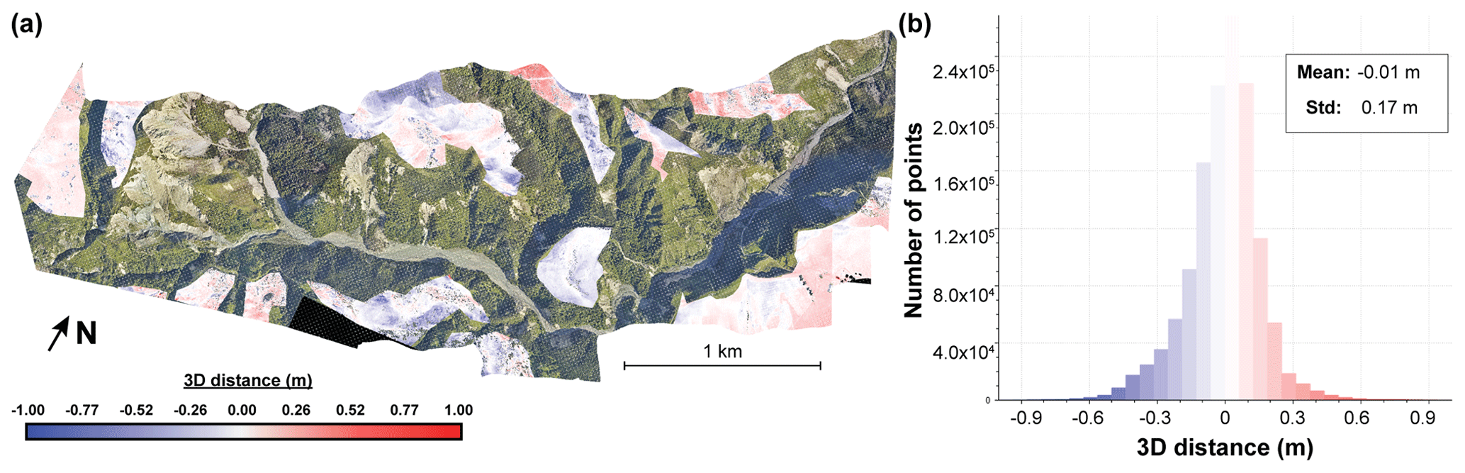
Figure 4(a) Map of 3D-M3C2 distances on stable areas and (b) the associated histogram. The map only displays 3D-M3C2 distance in the areas chosen as stable for ICP registration and shows the post-earthquake orthoimage otherwise (Aerial Surveys, 2017).
3.4.2 Geomorphic change detection
The registration error reg is then employed in a first application of 3D-M3C2, using the predetermined projection scale d= 5 m, to estimate the spatially variable LoD95 % according to Eq. (2). For core points in low-point-density areas, where a confidence interval could not be estimated due to insufficient points, a second application of 3D-M3C2 is performed at a larger projection scale d= 10 m. These core points generally correspond to ground points under canopy on steep slopes and represent 9.5 % of the entire area and 12 % of steep slopes prone to landsliding. Significant geomorphic changes at the 95 % confidence interval are then obtained by considering core points with a 3D-M3C2 distance larger than the LoD95 %. Significant geomorphic changes can be associated with any geomorphic processes, including landsliding, but also with fluvial erosion and deposition. Changes located in the river bed, and likely specifically related to river dynamics and not to landslide deposits, are manually removed using the post-EQ orthoimage. Along with the selection of the stable areas, this is the only manual phase of the workflow.
3.4.3 Landslide source and deposit segmentation
Core points with negative and positive significant changes are first separated into two distinct point clouds of sources and deposits, respectively. A vertical-M3C2 is performed on each of these point clouds to estimate the volume of landslide sources and deposits (see Sect. 3.3.4). As for any 2D landslide inventory, a critical component of the workflow is to segment each point cloud into individual landslide sources and areas. Segmenting complex patterns of erosion and deposition in 3D, with a very wide range of sizes, is still a challenge. Here, for the sake of simplicity we use a classical clustering approach with a 3D connected component labeling algorithm (Lumia et al., 1983), available in CloudCompare (Fig. 3c). The point cloud is segmented into individual clusters based on two criteria: a minimum number of points or surface area (in our case), Amin, defining a cluster and a minimum distance, Dm, below which neighboring points, measured in a 3D Euclidean sense, belong to the same cluster (Lumia et al., 1983). Amin was set to 20 m2 to be consistent with the area of the projection cylinder used to average the point cloud position in the M3C2 distance calculation, 19.6 m2 with d= 5 m. Dm is an important parameter which, if an overly large value is chosen, will favor landslide amalgamation in identical clusters, and if an overly small value is chosen, in relation to the core point spacing, may over-segment landslides. In any case, Dm must be larger than the core point spacing. As there is no objective way to a priori choose Dm, we explore various values and choose Dm= 2 m as an optimal value between landslide amalgamation and over-segmentation. The impact of Dm on the statistical distribution of landslide sources is addressed in Sect. 5.
We note that density-based clustering algorithms based on DBSCAN (Density-Based Spatial Clustering of Applications with Noise; Ester et al., 1996) have been used for 3D rockfall inventory segmentation (e.g., Benjamin et al., 2020; Tonini and Abellan, 2014). These algorithms separate dense clusters of points, considered as areas of coherent topographic change, from areas of low point density, considered as noise. As shown in the Supplement (Sect. S2), density-based clustering approaches do not yield a significantly better segmentation than a connected component algorithm. However, they have several drawbacks ranging from slow computation time, to less intuitive selection of parameters. Therefore, we have not used density-based clustering in our analysis.
3.4.4 Landslide area and volume estimation
While 3D normal computation is optimal to detect geomorphic changes, it is not suitable for volume estimation which requires the consideration of normals with parallel directions for a given landslide. Considering 3D normals can lead to “shadow zones”, due to surface roughness, which would result in a biased volume estimate (Fig. 3a). Therefore, distances and, in turn, volumes are computed by using a vertical-M3C2 on a grid of core points corresponding to the significant changes (Fig. 3b). As the core points are regularly spaced by 1 m, the landslide volume is simply the sum of the vertical-M3C2 distances estimated from the individualized landslides. While the distance uncertainty predicted by the vertical-M3C2 could be used as the volume uncertainty, it significantly overpredicts the true distance uncertainty due to nonoptimal normal orientation for the estimation of point cloud roughness on steep slopes (i.e., the roughness is not the detrended roughness). Thus, for each landslide source and deposit, we compute the volume uncertainty from the sum of the 3D-M3C2 uncertainty measured at each core point, not the vertical-M3C2 uncertainty. The volume uncertainty is specific to each landslide source and deposit and depends on the local surface properties, such as roughness, the number of points considered and the global registration error, but not on the volume itself. For each individual landslide source, the area A is obtained by computing the number of core points inside the source region. This represents the vertically projected area which is also consistent with the existing literature based on 2D studies of landslide statistics. The difference between planimetric area and true surface area (i.e., measured parallel to the surface) is addressed in Sect. 5.
3.5 Treatment of false detections
Owing to the simplified formulation of the LoD95 % (Eq. 2), it is possible for spatially correlated errors to create patches of statistically significant change that would appear after segmentation as false landslide detection (Fig. 5). Hence, the inventory after segmentation is provisional. The workflow has a classification step aiming at separating real landslides from false detections using patch-based metrics. As the pre-EQ lidar shows ground classification errors that would create false landslide sources (i.e., apparent negative change; Fig. 5a), and as we are specifically interested in the scaling relationships of sources, we focus on obtaining the best classification for sources and then simply use the proximity to the predicted true landslides sources to select real deposits. To construct the final landslide inventory, we apply the following steps:
-
labeling of at least 60 % of the provisional source inventory as actual landslide sources and false detections;
-
evaluation of the classification potential of various filtering metrics;
-
determination of the optimal filtering metrics based on a classification performance index;
-
application of the optimal filtering metrics to classify the provisional landslide source inventory in predicted landslides and predicted false detections.
As the pre-EQ lidar data quality (point density and classification) is significantly worse in forests than in forest-free areas, we carry out step 2 and 3 for provisional landslide sources located in forested and forest-free areas separately. Forest areas are defined based on the number of laser returns of the post-EQ dataset (Fig. S4). This corresponds to the number of targets a laser pulse has intercepted. For forest-free areas, this number is one, as the laser only hits the ground. However, in forested areas this number is expected to be greater than one, as tree elements create additional echoes before the laser hits the ground. Thus, for each core points, we calculate the average number of laser returns in a neighborhood of 2.5 m, to be consistent with the projection scale d, using the post-EQ lidar point cloud, which has the best canopy penetration. We then consider that any core point with an average number of laser returns equal to or higher than two is in forested areas.
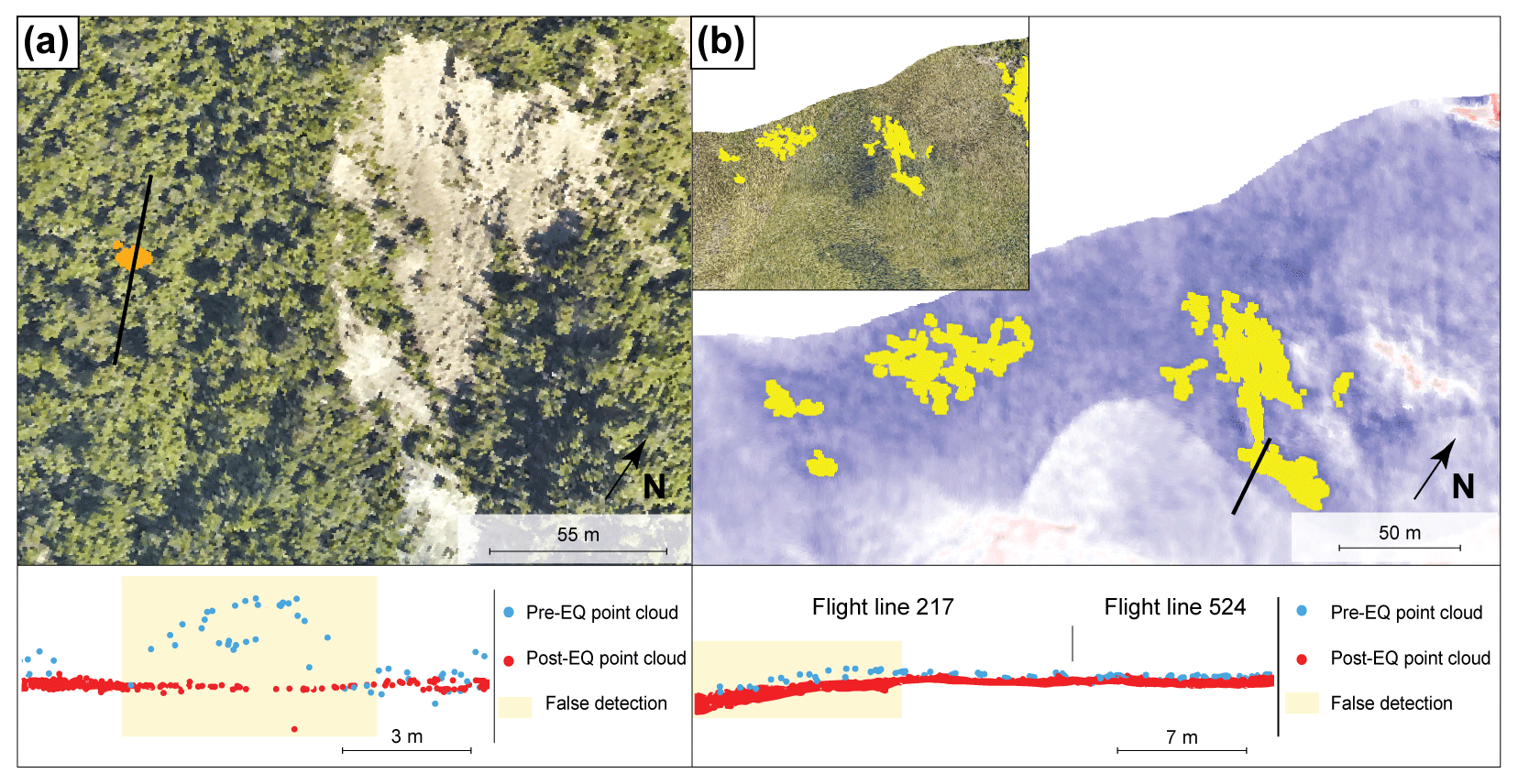
Figure 5Illustration of two types of labeled false detections. (a) A false detection located in a forest due to vegetation incorrectly classified as ground in the pre-EQ point cloud. The false detection is overlaid on the post-EQ orthoimagery (Aerial Surveys, 2017). The apparent negative topographic change creates a source. Note the limited penetration of the pre-EQ lidar in the dense evergreen forest that makes ground classification extremely difficult. (b) A false detection due to pre-EQ intra-survey registration errors. Yellow points on the post-EQ orthoimagery (Aerial Surveys, 2017) and the M3C2 distance field indicate patches of significant change that are a false detection. They occur due to a complex combination of intra-line errors related to time-dependent attitude and position errors and intra-survey flight-line registration error. Flight line 524 appears to be correctly registered to the post-EQ data, but flight line 217 is slightly misaligned, which increases the likelihood of significant change detection.
3.5.1 Construction of a labeled source inventory
The reference labeled source inventory is created with two classes, actual landslide source and false detection, according to the following procedure. We first manually label all of the provisional landslide sources with an area higher than 200 m2, as they are expected to correspond to the largest part of the total volume and are therefore critical. Provisional landslide sources with A < 200 m2 are then divided into 20 m2 area ranges. Following this, we choose to sample and label 60 % of the provisional landslide sources located in each area range in order to be representative of the provisional inventory and avoid a size bias. Attention has been paid to ensuring spatially uniform and equally distributed sampling between provisional landslide sources located in forested and forest-free areas.
The labeling of actual landslide sources and false detections is based on a visual inspection of the pre-EQ and post-EQ orthophotos, of the pre-EQ and post-EQ lidar point clouds, and of the 3D-M3C2 field and the provisional deposit inventory. We consider an actual landslide source according to the following criteria:
-
One of the following signs of mass movement is visible on orthoimagery – (1) a drastic change in color between the pre-EQ and post-EQ orthophotos due to avalanches, debris flows, landslides or rockfalls, or (2) the presence of scars.
-
The structure of the two point clouds does not show high local points due to the misclassification of vegetation (Fig. 5a).
-
The surrounding 3D-M3C2 field does not show a large constant value indicative of a locally incorrect registration (Fig. 5b)
-
The provisional source can be associated with at least one downstream provisional deposit within a radius of 30 m.
Not all criteria have to be met simultaneously. Uncertain provisional landslide sources have been labeled as false detection. The resulting labeled inventory is then used as a reference to evaluate the filtering performance.
3.5.2 Definition of filtering metrics
As false detections mainly emerge from the errors in the data in relation to the amplitude of a real topographic change that we aim to capture, we first choose to analyze three metrics based on the 3D-M3C2 calculation: (1) the maximum 3D distance, (2) the mean LoD95 % and (3) the mean signal-to-noise ratio (SNR). We expect the maximum 3D distance to discriminate between deep actual landslide sources and low-amplitude false detections arising from flight-line misalignments and residual registration errors characteristic of false detections in forest-free areas (Fig. 5b). As the LoD95 % is a direct measure of the quality of the data (point density and roughness), classification errors of vegetation should be characterized by a significantly higher mean LoD95 % than actual landslide sources. The SNR is defined as the ratio between the 3D-M3C2 distance and the associated LoD95 % for each core point. This measure can be used as a confidence metric for each source.
We also choose to take advantage of the ability of the 3D differencing approach to detect deposit areas to analyze the closest deposit distance (CDD). The CDD is defined for each provisional source as the closest downslope distance to a provisional deposit along the flow path using a D8 (deterministic eight-node) algorithm (Fairfield and Leymarie, 1991). This distance is calculated from the post-EQ DEM with the MATLAB-based TopoToolbox software (Schwanghart and Scherler, 2014).
Metrics with the best potential are then tested to determine an optimal configuration of filtering metrics that best remove false detections while retaining the maximum number of actual landslide sources. The resulting predicted source inventory is then employed to filter the provisional landslide deposit inventory by selecting the deposits that are connected to an upstream predicted landslide source along the flow path using TopoToolbox (Schwanghart and Scherler, 2014). The resulting inventory is called the predicted deposit inventory.
3.5.3 Definition of a classification performance index
To estimate the performance of the filtering metrics, we use the balanced accuracy (BA; Brodersen et al., 2010; Brodu and Lague, 2012), defined as the average accuracy obtained on the two predicted classes:
where, in our case, TPrate represents the percentage of correctly classified actual sources compared with the total labeled actual sources. Similarly, TNrate represents the percentage of correctly classified false detections compared with the total labeled false detections. This index not only reflects the overall performance of the filtering but also how TPrate and TNrate are balanced, thereby avoiding a biased representation of the filtering accuracy by the most frequent class. High values of BA are obtained when TPrate and TNrate are high and balanced. The BA can be estimated based on the number, the area or the volume of the predicted landslides (BAn, BAa and BAv, respectively), and we define BA as the mean of the BAn, BAa and BAv. By exploring a range of values for each filtering metric, we find the value that maximizes BA. Given the limited number of metrics that we use at once (a maximum combination of two), we did not use machine learning approaches to train the classifier.
3.6 Comparison with a manually mapped inventory based on orthoimagery
To estimate the potential in terms of landslide topographic change detection between the 3D-PcD method (3D-predicted inventory) and a traditional approach, we created a second inventory (2D inventory) by manually delineating landslide sources based on a visual interpretation of the pre- and post-EQ orthoimages, looking for texture change consistent with landslide scars. The lidar data were not used in the process, and the map maker did not have a detailed knowledge of the 3D-predicted inventory. Deposits were not mapped. The 2D and 3D landslide source inventories were then compared in terms of the number of landslides and the intersection of mapped surfaces in planimetric view using GIS software. For source areas only detected by manual mapping, we define four classes: (1) areas located on deposit zones detected by the 3D-PcD method, (2) areas under the LoD95 %, (3) areas filtered by the minimum area of 20 m2 and (4) areas filtered by the application of the optimal filtering metrics. For areas only detected by the 3D-PcD method, we distinguish landslide areas located in three land cover classes: (1) forest, (2) bare-rock and (3) other land covers. Forested areas are defined according to the number of returns of the post-EQ lidar (see Sect. 3.5), whereas bare rocks are delineated manually on the orthoimages. We finally analyze the proportion of areas only detected with the 3D-PcD approach that are connected to a landslide source in the 2D inventory.
4.1 Geomorphic change and results of the segmentation
The map of 3D-M3C2 distances (Fig. 6a) prior to statistically significant change analysis and segmentation provides a rare insight into topographic changes following a large earthquake. At first order, it highlights areas of coherent patterns of large (3D-M3C2 > 4 m) erosion (i.e., negative 3D distances) and deposition (i.e., positive 3D distances) located on hillslopes and corresponding to major landslides. Simple configurations with one major source area and a single deposit area can easily be recognized. A more complex pattern of intertwined landslides and rockfalls occurs on a bare-rock surface in the western part of the study area, with a large variety of source sizes and apparent aggregation of deposits. Most of the deposits are located on hillslopes; however, the deposits of three large landslides have reached the river and altered its geometry. At second order, a variety of patches of smaller amplitude (< 2 m) are visible on hillslopes. Erosion–deposition patterns in relation to fluvial activity can be documented on the river bed. The flight-line mismatch, identified during the preliminary quality control, leads to low-amplitude and long-wavelength patterns of negative and positive 3D distances, notably visible in the central northern part of the study area.
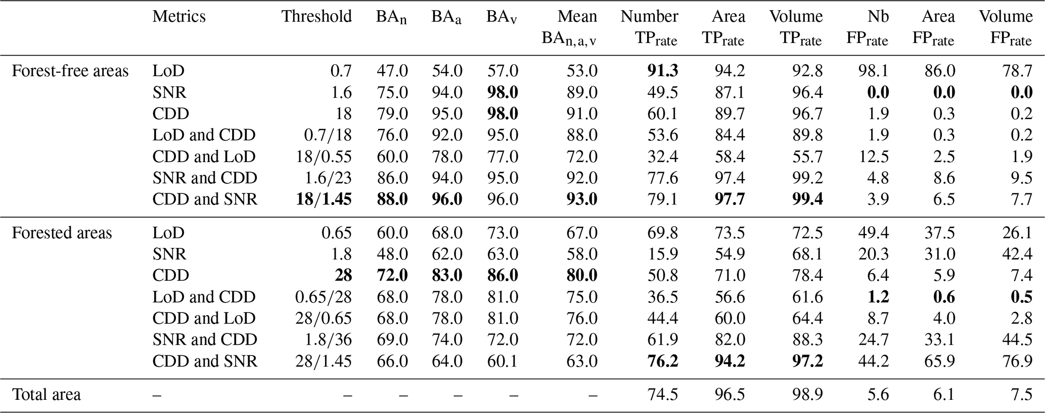
The area extent of significant changes, where the absolute amplitude of change is greater than LoD95 %, represents 13 % of the study area (Fig. 6b). Using the strict definition of the two-tailed statistics in Eq. (2) reduces the number of statistically significant points by ∼ 50 000 points, which is a 6.6 % reduction in the statistically significant area of change. After the manual removal of changes in the fluvial domain related to fluvial processes, the maximum 3D-M3C2 distance in significant change areas is −29.46 ± 1.00 m. Due to surface roughness, the minimum LoD95 % observed is 0.40 m.
The point cloud of significant changes is segmented to identify the provisional landslide sources and deposits. During this step, clusters smaller than the detection limit of 20 m2 are removed. They account for an area of 25 007 m2, which is 3.5 % of the total area of significant change. The provisional inventory contains 1118 sources and 698 deposits for a total of 320 170 and 312 471 m2, respectively. The resulting provisional landslide volume ranges from 2.27 ± 17.4 to 169 843 ± 20 598 m3 for source areas, with a total of 784 689 ± 179 608 m3, and from 1.3 ± 24.08 to 151 535 ± 15 301 m3 for deposits, with a total of 975 309 ± 171 578 m3. Considering that the minimum LoD95 % observed using the 3D method is 0.40 m and that the minimum landslide area is 20 m2, the minimum volume that we can confidently measure should be 8 m3, a value higher than the observed minimum volumes. A total of 5 provisional landslide source and 16 provisional deposits are smaller than 8 m3. They correspond to peculiar cases of very small landslides where either positive or negative 3D distances close to the LoD95 % are positive or negative when measured vertically and, thus, reduce the apparent volume of the material. The uncertainty in the total volume estimation represents 23 % for sources and 18 % for deposits.
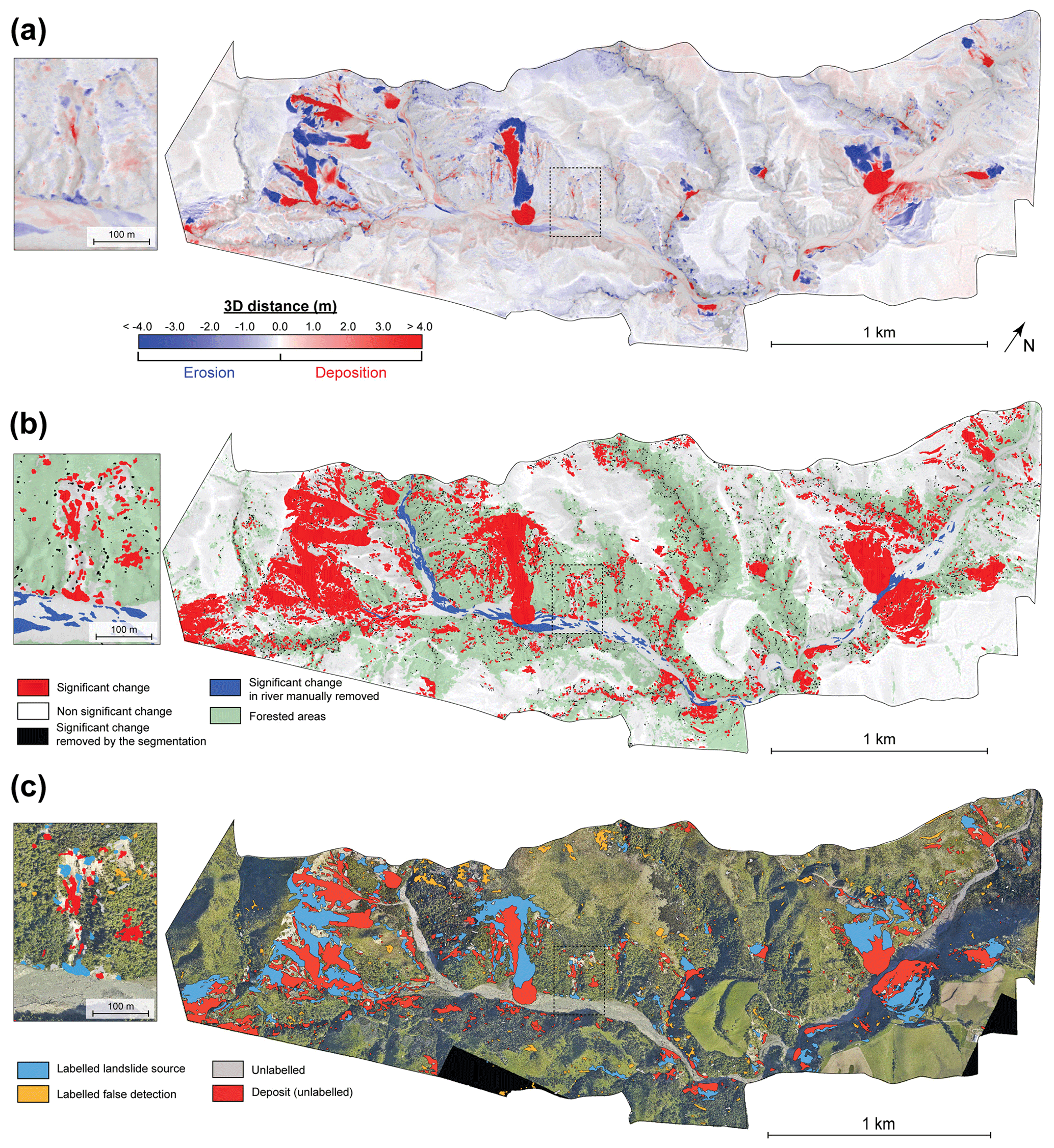
Figure 6Maps of the different steps of the workflow to generate the provisional landslide inventory. Panel (a) shows the 3D-M3C2 distances from the geomorphic change detection step. Panel (b) displays significant changes (> LoD95 %), indicating areas filtered in the river and by the segmentation procedure. The forested areas calculated as a function of the number of lidar returns on the post-EQ data are also indicated in green (see Sect. 3.5). Panel (c) shows the provisional inventory after the application of a minimum area of 20 m2. The labeled source inventory is also shown. Results are overlaid on the post-earthquake orthoimagery (15 December 2016, Aerial Surveys, 2017).
4.2 Removal of false detections and the 3D-predicted inventory
4.2.1 Labeled inventory characteristics and potential of filtering metrics
The labeled inventory contains 66 % of the provisional landslide sources with 384 actual landslide sources and 355 false detections. In forest-free areas, 321 actual landslide sources have been labeled and 104 false detections are noted, indicating a false detection prevalence of 24.5 %. The mean area of false detections is 174 m2, with a minimum of 20 m2 and a maximum of 2417 m2. In forested areas, only 63 actual sources have been labeled for 251 false detections, resulting in a false detection prevalence of almost 80 %. The mean area of false detections in these regions is 90 m2, with a minimum of 20 m2 and a maximum of 1039 m2. The prevalence of 24.5 % in non-forested areas is indicative of the combined effect of elevation errors due to the combination of intra-flight-line elevation errors, intra-survey flight-line registration errors and the inter-survey registration error. The increased prevalence in forests is due to ground classification errors. Considering the entire labeled inventory, the prevalence of false detections decreases with size from 60 % for the 20–40 m2 class to 10 % for A > 2000 m2 (Fig. 7). If false detections were not removed, their prevalence and size dependency would strongly bias the landslide source area distribution towards small sizes.
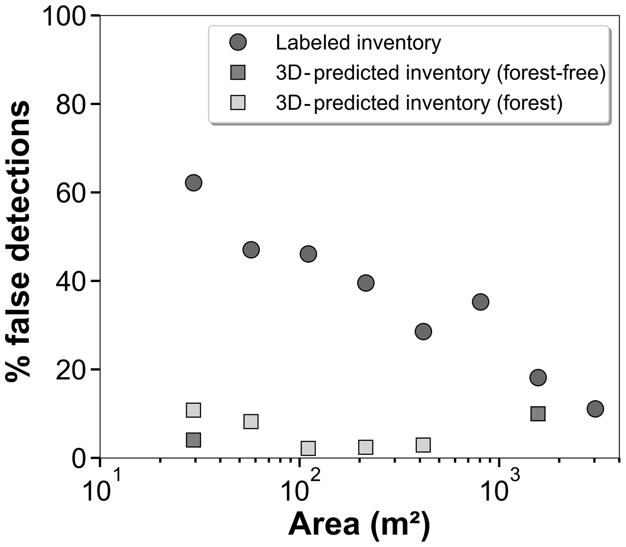
Figure 7The proportion of false detections in the labeled inventory and the 3D-predicted inventory (forest-free and forested areas) with source area.
To determine the potential of the patch metrics to remove false detections, we analyze the cumulative density distributions of each metric for actual landslide sources and false detections (Fig. 8). In forest-free areas, the maximum 3D distance and the LoD95 % of the labeled inventory show the weakest potential to remove false detections, as the cumulative density functions (CDFs) of false detections and landslide sources are similar (Fig. 8a, b). However, the CDFs of the SNR and CDD show different behavior for landslide sources and false detections (Fig. 8c, d). About 60 % of landslide sources are characterized by a mean SNR higher than 1.5, and about 75 % have a CDD lower than 30 m. On the contrary, all false detections are characterized by a mean SNR below 1.5, and about 90 % have a CDD higher than 30 m. The low SNR observed for false detections is due to the low amplitude (70 % of false detection areas have 3D-M3C2 < 1 m) of the type of elevation errors found in forest-free areas (Fig. 5b). Similarly, these type of errors are not expected to produce a coherent pattern of upslope erosion and downslope deposition over short distances which is similar to that produced by landslides. Thus, the SNR and the CDD constitute the best metrics to differentiate between actual landslide sources and false detections in forest-free areas.
In forested areas, where ground classification errors are present (Fig. 5a), false detections are characterized by a higher maximum 3D distance and mean LoD95 % than landslide sources (Fig. 8a). This is related to ground classification errors which correspond to 3D-M3C2 distances of the order of the forest canopy height (i.e., several meters), with high LoD95 % due to low point density and high point cloud roughness. However, the CDFs of the maximum 3D distance are not distinct enough for the two classes for this metric to be used in the classification. The CDFs of the mean LoD95 % show that actual sources are characterized by a maximum mean LoD95 % of 0.9, whereas about 15 % of the false detections have a higher mean LoD95 %. In this context, the SNR is not an interesting classifying metric, as false detections in forests have a larger M3C2-distance than non-forested areas, resulting in a similar CDF for sources and false detections. The CDFs of CDD are similar to forest-free areas, highlighting the good classification potential of this metric.
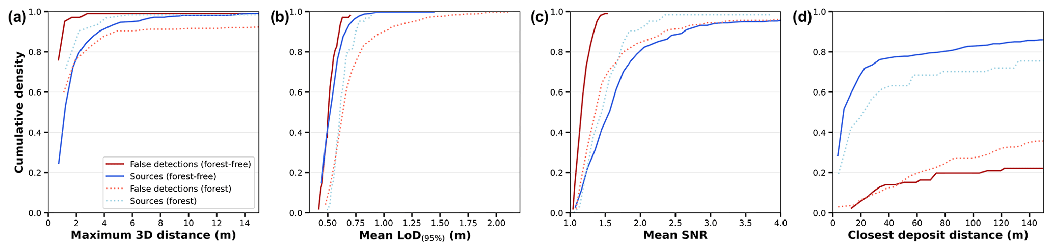
Figure 8Cumulative density functions of the different metrics introduced in Sect. 3.5.2 using the labeled inventory. The distributions are presented according to landslide sources and false detections in forest-free and forested areas.
We choose to test the mean LoD95 %, the mean SNR and the CDD metrics to classify the provisional landslide source inventory. For each test, we select provisional landslide sources below a threshold TLoD and TCDD when using the mean LoD95 % and the CDD, respectively, and above a threshold TSNR when the mean SNR is considered. Different combinations of these metrics have been tested to determine an optimal classification (Table 2).
4.2.2 Optimal filtering metrics
Table 2 reports the BA for the various metrics and forest environments, as well as the true positive rate (i.e., the fraction of landslide source preserved in the predicted inventory) and the false positive rate (i.e., the fraction of false detections that are not removed out of all false detections). We choose the optimal configuration of filtering metrics corresponding to the highest BA (Table 2), as it reflects the best balance between false detection removal and the preservation of true landslide sources in terms of number, area and volume.
In forest-free areas, the lowest performance is obtained when the mean LoD95 % is applied alone or in combination with the mean SNR and the CDD (mean BA < 88 %), as expected based on the analysis of CDFs (Fig. 8b). Conversely, the mean SNR and the CDD provide better performance (mean BA > 88 %) when applied alone or in combination. When applied alone, they preserve 96 % of the total actual landslide sources. However, while the mean SNR (TSNR= 1.6) removes all false detections (FPrate= 0), the CDD (TCDD= 18 m) better preserves the actual landslide source number (TPrate= 60 %) and area (TPrate= 90 %). The optimal combination is obtained when first applying TCDD= 18 m followed by TSNR= 1.45, resulting in a mean BA of 93 %. This combination best preserves the area and volume of labeled landslide sources with a TPrate of 79.1 %, 97.7 % and 99.4 %, respectively. The number, area and volume of false detections remains low with a FPrate of 3.9 %, 6.5 % and 7.7 %, respectively. The prevalence of false detection after the classification of the inventory is 1.5 % with respect to number, 0.48 % with respect to area and 0.15 % with respect to volume.
In forested areas, the lowest performance is obtained for the SNR with a BA of 58 %. However, in combination with the CDD, it best preserves the number, area and volume of the labeled landslide sources with a TPrate of 76 %, 94 % and 97 %, respectively, but it fails to remove false detections (FPrate in volume = 44 %). The combination of filtering metrics that best removes false detections is obtained when 0.65 and TCDD= 28 m are applied, but it is at a higher filtering cost with respect to labeled landslide sources (TPrate= 1.2 %). The best performance is obtained by applying only TCDD= 28 m with a mean BA of 0.80, and it corresponds to the best balance in terms of number, area and volume of landslide sources preserved and false detections removed. The prevalence of false detection after the classification of the inventory is 33 % with respect to number, 13.3 % with respect to area and 12.5 % with respect to volume.
Finally, after application of the optimal configuration of filtering metrics in forested and forest-free areas, we obtain a total labeled predicted source inventory preserving 75 % of landslide sources and 96 % and 99 % of the corresponding total area and volume, respectively (Table 2). False detections remaining in the labeled predicted inventory represent 6.5 % of the total number of labeled predicted sources, whereas they only represent 1 % of the total area and 0.45 % of the total volume.
Table 2Statistics of the labeled inventories according to each combination of filtering metrics. FPrate is given as FPrate = FP (FP + TN), where FP represents the false detection present in the labeled predicted inventory. Bold values highlight the best result in each column for the given class (forest-free and forested areas).
4.2.3 The 3D-predicted inventory
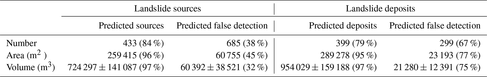
The optimal filtering metrics are then applied on the entire provisional source inventory. Hereafter, we call the resulting filtered inventory the “3D-predicted inventory” and use this data to perform subsequent analysis. This inventory contains a total of 433 sources and 399 deposits, with many sources sharing the same deposits at the toe of hillslopes (Fig. 9, Table 3). The filtering step successfully removed false detections located on stable areas, so that no landslide source is predicted on stable areas. For sources, the mean absolute vertical-M3C2 distance is 2.82 m, the standard deviation is 2.99 m and the maximum absolute value is 23.06 ± 0.70 m. For deposits, the mean absolute vertical-M3C2 distance is 3.33 m, the standard deviation is 3.66 m and the maximum absolute value is 27.9 ± 0.50 m. The area of detected landslides ranges from 20 to 40 475 m2 for sources and from 20 to 27 782 m2 for deposits, and the total source and deposit areas are 259 415 and 289 278 m2, respectively. The resulting individual landslide volume ranges from 0.58 ± 11.53 to 169 725 ± 20 598 m3 for source areas, with a total of 724 297 ± 141 087 m3, and from 7.95 ± 9.83 to 151 717 ± 15 301 m3 for deposits, with a total of 954 029 ± 159 188 m3 (Table 3). The uncertainty in the total volume estimation represents about 19 % for sources and 17 % for deposits. The filtering approach removes 685 provisional sources and 299 provisional deposits. This represents 19 % and 7.4 % of the total provisional source and deposit area and 7.7 % and 2.2 % of the total volume, respectively.

Figure 9Map of the 3D-predicted inventory with vertical-M3C2 distances after the application of TCDD= 18 m and TSNR= 1.45 in forest-free areas and TCDD= 28 m in forested areas. The landslide inventory is overlaid on the post-EQ orthoimagery (15 December 2016, Aerial Surveys, 2017). Landslide sources are in blue, and landslide deposits are in red.
Table 3Statistics of the predicted inventory with the percentage located in forest-free areas given in parentheses.
4.3 The 3D-predicted versus the 2D landslide source inventory
In the following analysis we separate two types of errors: detection errors, corresponding to landslides present in only one of the 2D and 3D inventories, and delimitation errors, corresponding to differences in the planimetric outline of landslides. A total of 258 landslide sources, hereafter referred to as “2D-sources” as opposed to “3D-sources” derived from 3D-PcD, were mapped from visual inspection of pre-EQ and post-EQ orthoimages (Fig. 10b). The 2D-sources represent a total area of 146 641 m2 (Table 4), with a minimum area of 6 m2 and a maximum of 19 784 m2. The minimum area detected shows that the resolution capability of the 2D inventory is finer than the 3D-PcD workflow. From the 258 2D-sources, 193 intersect 3D-sources, and 65 are not detected by the 3D-PcD method. These 65 2D-sources range from 12 to 645 m2 with 69 % being smaller than 100 m2. However, 22 are actual deposits in the 3D inventory, highlighting detection errors in the 2D inventory. These detection errors represent 14.8 % of the surface of the 2D inventory and are removed in the following, leading to 43 2D-sources not detected by the 3D-PcD method. Thus, the 3D-PcD method detects 74.8 % of the 2D-sources and 57.2 % of the total surface of the 2D inventory (Table 4). The 43 2D-sources not detected by the 3D-PcD method correspond to 39 2D-sources located in areas with no statistically significant change (i.e., 3D-M3C2 distance < LoD95 %) and 4 2D-sources removed by the filtering step of the workflow. In terms of planimetric surface area, the area not captured by 3D-PcD is overwhelming dominated by non-statistically significant change (42 % of the total 2D-sources surface is < LoD95 %), as opposed to the filtering based on the CDD and SNR (0.4 %) or the minimum detectable size (0.3 %). The surface of non-statistically significant change corresponds to delimitation errors located on the edges of sources and deposits, owing to the averaging effect of the M3C2 approach, and the transition between landslide sources and deposits (Fig. 10c). The volume missed in 3D-sources was computed by using the intersection between the outline of the 2D-sources not shared in the 3D inventory and the vertical-M3C2 field of the core points. We find that the volume that would be missed in the 3D inventory is 2.2 % of the total volume of 3D-sources.
While 193 2D-sources are common to 3D-sources, this corresponds to 182 3D-sources owing to the difference in landslide segmentation in the two inventories (Fig. 10a). The 2D inventory misses 42 % (251) of the landslide sources detected in the 3D inventory, including landslides as large as 11 902 m2 (blue polygon in the frame of Fig. 10a). The detection errors are predominantly in bare-rock areas (116, 46 % of detection errors) and other land covers (87, 35 % of detection errors) where the prevalence of false detections in the 3D-PcD dataset is expected to be extremely low (1.5 %); thus, the missing landslides in the 2D inventory are not potential false detections. The missed landslides can be very large landslides occurring within pronounced shadows in the post-EQ orthoimage, where the topographic change is mostly vertical (Fig. 10c). Missed landslides also occur in forested areas, although with a lower proportion (48, 19 % of detection errors); however, we could expect from the classification of the labeled data that a third of these missing landslides may be false detection of the 3D inventory. It was observed that 72 % of the total surface of 3D-sources is not detected in the 2D inventory, with a small fraction (17 %) under forest, 39 % on bare rock and 44 % on other land covers (Table 4 and Fig. S5). The landslide sources in this latter domain should be generally visible owing to a strong spectral contrast between pre-EQ vegetation and post-EQ rock surfaces. However, the large source of disagreement is explained by the incorrect delimitation of upslope topographic subsidence related to large scars as well as the underdetection of vertical subsidence related to translational and rotational landslides (Fig. 13b). These vertical movements of meter-scale amplitude or less do not correspond to a clear change in orthoimagery texture nor do they create scarps that are too small or not easily detectable if they do not generate a shadow. Similarly, large subsiding areas corresponding to retrogressive failure plane development or reactivation can be detected under forest but are totally missed in the 2D inventory (Fig. 10c). Detection and delimitation errors contribute roughly equally to the 2D area underdetection (42 % detection error, 58 % delimitation error). The 2D-sources data miss 54 % of the total volume of the 3D-sources. In contrast to the missed planimetric surface area, the missed volume is predominantly on bare rock (34.2 %) and is about 3 times larger than in forest (10.6 %) or other land covers (13.4 %).
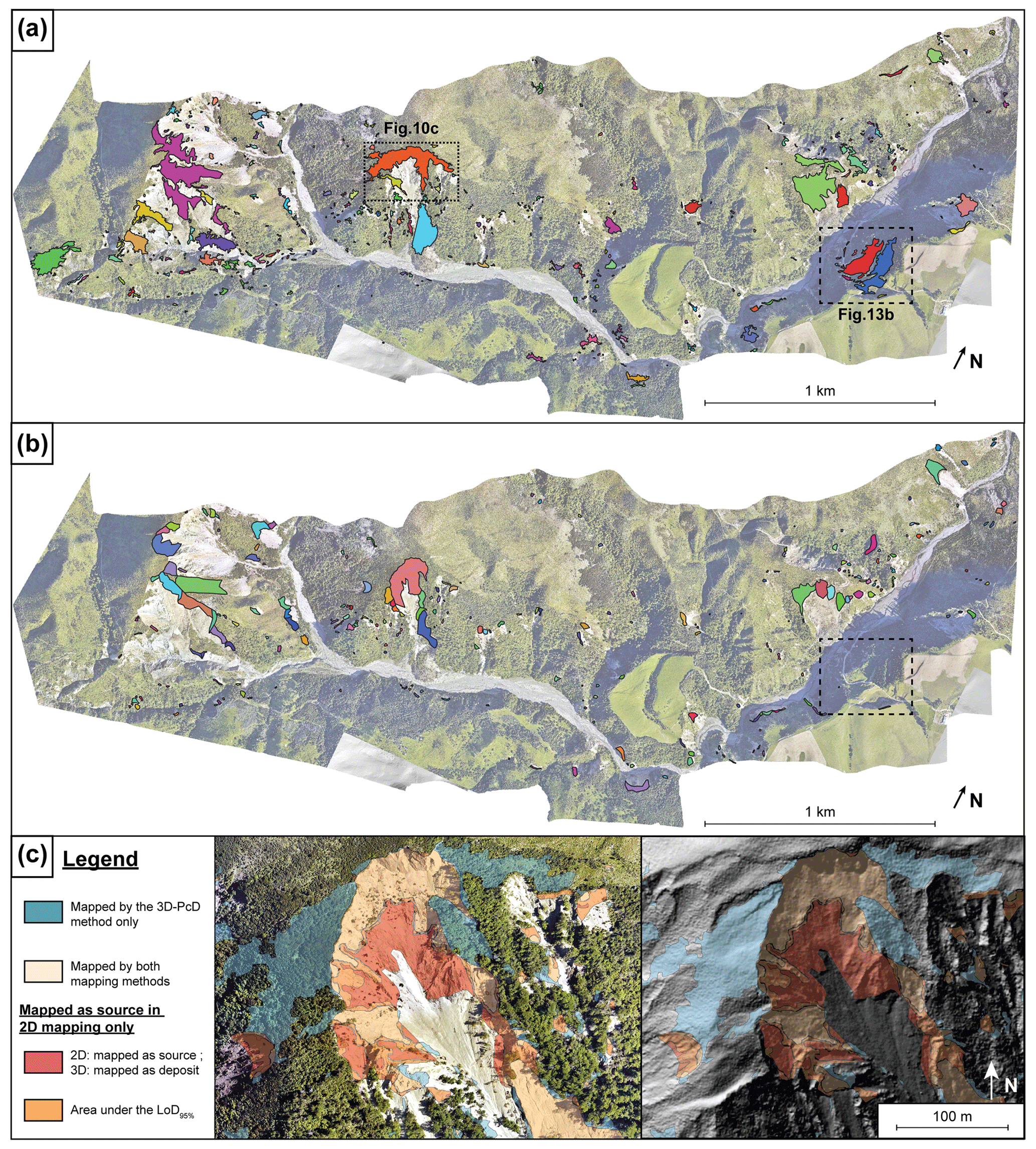
Figure 10Comparison between (a) the 3D-predicted inventory and (b) manual mapping based on 2D orthoimage comparison. Each landslide source is shown as a single colored polygon. Panel (c) shows a detailed comparison of typical mapping differences between the 2D and 3D approaches. Data are overlaid on the post-EQ orthoimagery (15 December 2016, Aerial Surveys, 2017) and the post-EQ DEM is shown on the right. Panel (c) also shows that the detected negative topographic change by the 3D-PcD method under a dense forested area is consistent with the development or reactivation of retrogressive failure planes with visible scarps in the hillshade view around the main landslide. The 2D orthoimagery cannot detect these mainly vertical changes under forest, which do not affect the texture of the image.
Table 4Summary of the comparison between the 2D- and the 3D-predicted landslide source inventories. For the 2D inventory, the percentages are calculated with respect to the corrected total in which the 2D sources corresponding to 3D deposits are removed. NA stands for not available.
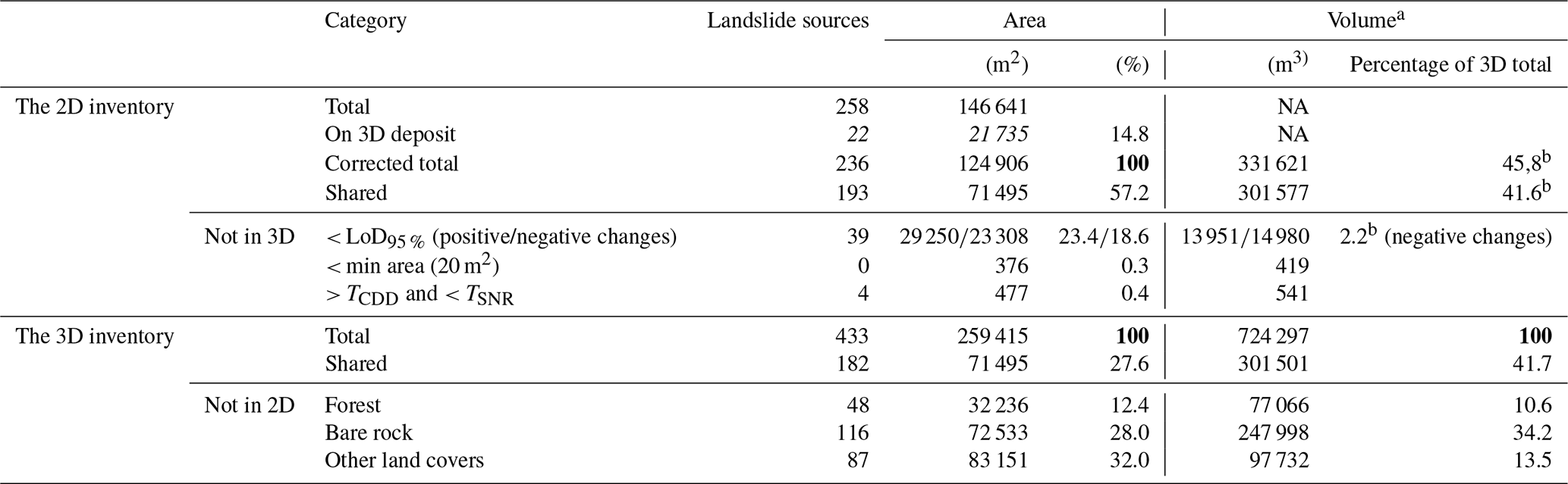
a The volumes for the 2D inventory are computed from the vertical-M3C2 of core points located within the sources delimitations. b The percentage represents the 2D volume of the class in comparison with the total volume of the 3D-predicted inventory.
4.4 Landslide sources area, depth and volume analysis
The area distribution of landslide sources is computed as follows (Hovius et al., 1997; Malamud et al., 2004):
where p(A) is the probability density of a given area range within a landslide inventory, NLT is the total number of landslides and A is the landslide source area. δNLT corresponds to the number of landslides with areas between A and A+δA. The landslide area bin widths δA are equal in logarithmic space.
First, the area distribution of landslide sources obeys a power-law scaling relationship, consistent with previous studies (e.g., Hovius et al., 1997; Malamud et al., 2004). The exponents are c= −1.76 ± 0.06 and c= −1.64 ± 0.03 for the 2D and 3D inventories, respectively (Fig. 11a). The distribution of the 2D inventory shows a cutoff from power-law behavior at around 100 m2, a peak probability at 20 m2 and a rollover for smaller landslide sizes. The landslide area distribution of the 3D-predicted inventory does not exhibit a rollover but slightly deviates from the power-law behavior around 40 m2. The distribution differs from that derived by Massey et al. (2020) in the broader Kaikōura region for which a cutoff appears at around 1000 m2 with a rollover at 100 m2.
The volume distribution of the landslide sources in the 3D inventory was defined using Eq. (44), replacing A with the volume V, and also exhibits a negative power-law scaling (Fig. 11b) that has the following form: p(V)=dVe. The exponent of the power-law relationship is e= −1.54 ± 0.07. A rollover is visible on the landslide volume distribution at around 20 m3.
With a direct measurement of landslide volume, it is possible to compute the volume–area relationship (Eq. 1; Simonett, 1967; Larsen et al., 2010) and to compare it with previous results from New Zealand (Larsen et al., 2010; Massey et al., 2020). Here, we determine V–A scaling coefficients using two methods: first, by fitting a linear model on log-transformed data and, second, by fitting a linear model on averaged log-binned data. While the first method leads to a V–A relationship best describing the volume of each landslide, the second one is not affected by the varying number of landslides in each landslide area bin and leads to a V–A relationship that best matches the total landslide volume. Using the first approach, we find a volume–area scaling exponent of , an intercept of m0.72 and a determination coefficient of R2=0.93 (Fig. 11c). Using the second method, we find , an intercept of m0.66 and a determination coefficient of R2=0.99. We also obtain a good correlation R2 of 0.86 and 0.80 with the relationships from Larsen et al. (2010) that were derived from soil landslides and from mixed soil landslides and bedrock landslides, respectively (Table 5). An R2 of 0.92 is obtained when considering the parameters of the V–A relationships of the Kaikōura region, derived by Massey et al. (2020), including all of their mapped landslides. Thus, at first order, the V–A relationships that we obtained are consistent with previous studies. However, if the relationships from Larsen et al. (2010) and Massey et al. (2020) were applied to our landslide area inventory, the total volume would vary from 0.346×10⁶ to 0.940×10⁶ m3 (Table 5), compared with the 0.724×10⁶ ± 0.141×10⁶ m3 that we estimate directly. The closest evaluation of the total volume is based on the Massey et al. (2020) V–A relationship that predicts a total volume of 0.600×10⁶ m3. The farthest evaluation from the total volume measured in 3D is the V–A relationship from Larsen et al. (2010) for all landslides (0.940×10⁶ m3), whereas their soil-dominated landslide relationship predicts less than a half of the total volume of the 3D inventory.
We presented the V–A relationship because it is classically used in coseismic volume estimates from 2D inventories; however, as the volume is the product of mean depth and area, the V–A relationship hides an indirect correlation with area that may hinder obscure subtle variations in depth with landslide size. The raw mean depth–area data show a large scatter for nearly all landslide areas. The log-binned data show a slight increase in depth with area. Using a power-law model, which is actually weakly constrained here, an exponent of 0.18±0.06 (R2= 0.87) is derived, which is consistent with the V–A relationship. The soil landslide relationships of Larsen et al. (2010) and Massey et al. (2020) are broadly consistent with the log-binned data (R2= 0.81 and R2= 0.75, respectively), but the mixed soil and bedrock landslide relationship of Larsen et al. (2010) exhibits a much larger scaling exponent, resulting in a poor correlation ().
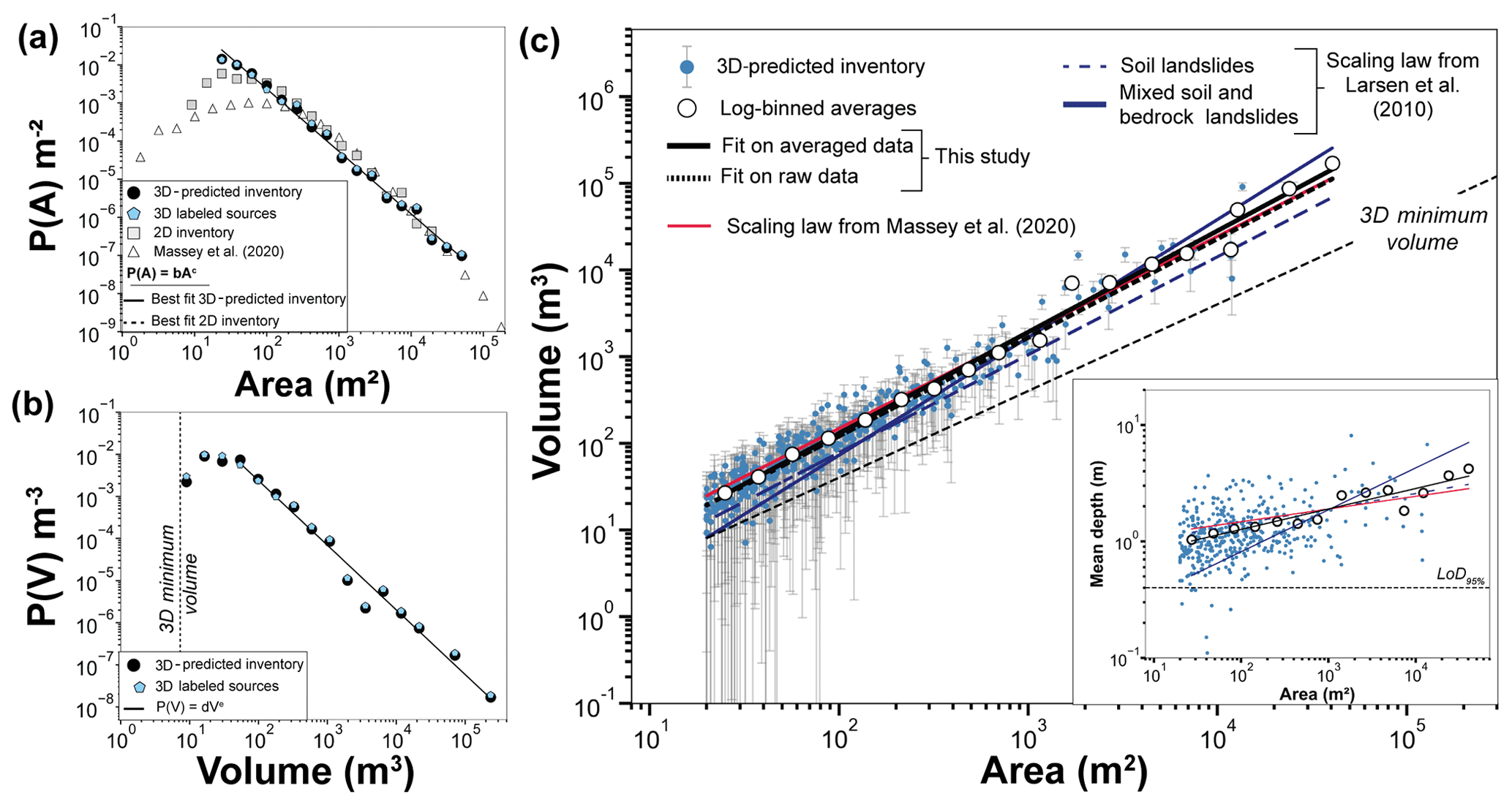
Figure 11Landslide source inventory analysis of the study area: (a) landslide area distribution of the 3D-predicted inventory, the labeled sources, the 2D inventory and Massey et al. (2020); (b) landslide volume distribution of both the 3D-predicted inventory and the labeled source inventory; (c) volume–area scaling relationships, showing the uncertainty in the volume and a comparison with the relationships from Larsen et al. (2010) and Massey et al. (2020) obtained in New Zealand. The landslide mean depth versus area is also presented in the inset in panel (c). All scaling parameter values are summarized in Table 5. Fits correspond to least squares fitting of a power law to log-binned data above a manually selected cutoff.
Table 5Power-law scaling parameter values of the relations shown in Fig. 11. Log α and γ are scaling parameters from the landslide volume–area relationship (Eq. 1). Units of α are [L(3−2γ)], with L in meters. The respective landslide source area and volume distribution coefficients are b and d, and the exponents are c and e, respectively. The coefficient of determination R2 is also given for each power-law fit function. The total volume refers to the application of the V–A relationship to the landslide areas of the 3D-predicted inventory.
a Direct measurement. b The exponent is estimated as γ-1, and the coefficient has units of [L(1−2γ)]. R2 is estimated using log-binned data.
The aim of this paper is to present a semiautomatic workflow, called 3D-PcD, for the detection and geometric characterization of landslide sources and deposits from repeated airborne lidar data. We specifically aim to overcome the impact of issues such as underdetection of landslides in inventories based on imagery analysis, landslide amalgamation and V–A relationship biases on total volume calculation. In the following, we discuss (1) the benefits and limits of the 3D-PcD method, (2) the benefits of 3D change detection to create landslide inventories, and (3) how 3D landslide inventories shed new light on the scaling properties of landslide sources.
5.1 The 3D point cloud differencing and landslide detection
5.1.1 Vertical versus 3D change detection capability, and the M3C2 algorithm
The importance of detecting changes in three dimensions (3D-M3C2), as opposed to vertically (vertical-M3C2), on steep slopes can be illustrated by an SSDS test applied to the post-EQ point cloud (Fig. 12). Typical of change measurement methods on rough surfaces with random point sampling (e.g., Lague et al., 2013), a nonzero mean distance is often measured, even though the two point clouds are samples of exactly the same surface. The distribution of measured distances is centered near zero, with means of and m for the vertical and 3D approaches, respectively. However, the 3D approach results in a standard deviation (σ= 0.05 m) that is 4 times smaller than that obtained by using vertical differencing (σ= 0.20 m). The map of difference shows that vertical differencing systematically results in much larger distances on steep slopes than the 3D approach, although they both yield similar low distances on horizontal surfaces.
We find that the 3D-PcD method offers a greater change detection sensitivity than classical vertical DoD. This difference is particularly important as it propagates into a lower level of detection and uncertainty in volume calculations. Using the M3C2 algorithm in three dimensions (Lague et al., 2013) also offers the benefit of accounting for spatially variable point density and roughness in estimating a distance uncertainty for each core point, which can be subsequently used in volume uncertainty calculation. For instance, 3D-M3C2 reduces the sensitivity of change detection in vegetated areas to a lower ground point density and potentially to a higher roughness due to vegetation misclassification. In turn, this advantage partially prevents the detection of false sources or deposits by using 3D-M3C2. By employing a regular grid of core points, as in Wagner et al. (2017), our workflow combines the benefits of working directly with the raw unorganized 3D data, as opposed to DoD where the relationship with the underlying higher-point-density data is lost. This approach also produces results with a regular sampling that can easily be used for unbiased spatial statistics, volume calculation and easy integration into 2D GIS software. Compared with DoD, if an interpolation is needed, it is performed on the results rather than on the original DEM and can lead to uncontrolled error budget management.

Figure 12Comparison between vertical differencing (vertical-M3C2) and 3D differencing (3D-M3C2) on the post-EQ point cloud, subsampled randomly two times to generate two point clouds of the same surface with different sampling techniques (same surface different sampling test). Panel (a) displays the resulting change detection maps of the two different techniques, and panel (b) presents the histogram of the computed distances with the two techniques.
5.1.2 Current limits of the method
Registration and elevation errors
A critical aspect of the comparison of 3D point clouds is their co-registration, in particular in the context of coseismic landsliding. In this study, a rigid transformation is applied to the datasets using an ICP algorithm (Besl and McKay, 1992), assuming that internal deformation induced by the earthquake is negligible. The 3D-M3C2 map does not exhibit any systematic horizontal shift north nor south of the Hope Fault. Thus, we conclude that internal deformation, if there was any, was below the typical registration error in our study area. For larger studied regions with internal deformation and in the absence of a 3D coseismic deformation model that could be applied to the post-EQ point cloud (e.g., Massey et al., 2020), our workflow should be applied in a piecewise manner with boundaries corresponding to the main identified faults or deformation zones. For landslide inventories following climatic events, the application to large datasets should be straightforward, as no significant internal deformation is expected. However, we note internal flight-line height mismatches of 0.13–0.20 m in the pre-EQ survey that are difficult to correct after data delivery and generate some apparent large-scale, low-amplitude topographic changes (Fig. 4, Table S1 and Sect. S2 in the Supplement). Interestingly, in the M3C2 calculation, flight-line mismatches are averaged out in the distance measurement but lead to a higher local point cloud standard deviation and, thus, to an increase in the LoD95 % and to a lower probability of incorrect topographic change detection. Despite significant flight-line mismatches in the pre-EQ dataset, using the SNR and CDD filtering approach efficiently removes the false detection source areas related to this issue in non-forested area. This highlights (1) the need for detailed quality control (e.g., by applying M3C2 on overlapping lines) to ensure the highest accuracy of the lidar data, (2) the importance of the statistical significance tests performed at the core point scale and (3) the need for confidence metrics at the landslide scale, to filter out a variety of potential false landslides. Ideally, a spatially variable model for point cloud errors and registration should be developed for each survey and combined into a more accurate and complete form of LoD than what the M3C2 approach currently offers (e.g., Glennie, 2008; Passalacqua et al., 2015). However, the position and altitude information of the sensor (e.g., smoothed best estimate of trajectory file) and raw lidar data are rarely available from lidar data repositories. Additionally, a dense network of GCPs is hard to get in mountainous environments. Thus, it is frequently impossible to reprocess the lidar data to improve their quality (e.g., Glennie et al., 2014) or to create a spatially variable registration and point cloud error model. This explains our choice of assuming a uniform registration error and estimating it empirically from intra-survey flight-line overlapping errors or inter-survey 3D-M3C2 distances over stable areas. As a result, we analyze the influence of the reg value on the landslide source population (see Sect. 5.2.2).
Landslide segmentation
The connected component segmentation is a simple, objective and rapid way to separate landslides in 3D that can be scaled up to much larger datasets. However, given the complexity of the 3D data, in particular the very large range of landslide sizes (i.e., 4 orders of magnitude in the studied case), it inevitably exhibits some drawbacks and is subject to improvement. In particular, landslide amalgamation occurs between two sources or deposits if two of their core points are closer than Dm (2 m in this study). Hence, landslides occurring on the two sides of a collapsed divide can be erroneously connected. This is the case for the largest landslide in our database which is located on the rock cliffs in the western part of the study area (Figs. 10a, 13a). In this example, the landslide source could reasonably be segmented into at least five smaller landslides. However, there does not seem to be a unique way to segment such a complex set of amalgamated events, even manually, underlining that landslide segmentation cannot currently be fully objective. As we aim to apply our workflow to very large datasets, potentially with several tens of thousands of landslides, and as false detection filtering needs to operate on segmented patches, automatic segmentation is a mandatory step. We have explored the use of fast implementations of a density-based spatial clustering algorithm derived from DBSCAN (Ester et al., 1996), which is an algorithm used for the segmentation of 3D point clouds of rockfalls and the removal of noisy points (e.g., Benjamin et al., 2020; Tonini and Abellan, 2014; details in Sect. S2). We applied OPTICS (Ordering Points To Identify the Clustering Structure; Ankerst et al., 1999), recently used for rockfall segmentation of 3D lidar data (Carrea et al., 2021), and HDBSCAN (Hierarchical Density-Based Spatial Clustering of Applications with Noise; McInnes et al., 2017), which has a better ability to detect clusters of various sizes compared with DBSCAN and is also much faster. However, none of these approaches managed to provide a significantly better segmentation of the largest landslides of our database, and the density probability of the source area that they produce is very similar to the one generated by a connected component approach. These approaches are, however, significantly longer to run than a connected component approach in CloudCompare (Sect. S2), and they have parameters which are less intuitive to set than Dm, which is a distance directly comparable to core point spacing. New segmentation approaches accounting for normal direction, divide organization and 3D depth maps of amalgamated sources are needed to improve the segmentation of complex cases. Manual segmentation can also be envisioned as a refinement after the predicted true landslide sources and deposits have been produced, but it is irreproducible and time-consuming when applied to very large datasets. We note, however, that segmentation issues do not affect the total landslide volume calculation in our study and that a sensitivity analysis of the impact of Dm shows that landslide source statistics are not severely affected by this parameter as long as it is close to the value that we have used (see Sect. 5.2).
Landslide volume calculation
Landslide volume is computed using vertical-M3C2 on regular core points. This facilitates volume calculation on potentially complex 2D landslide geometry but may lead to incorrect volume estimates on very steep slopes. However, the median slope of the source core points (measured on the pre-EQ surface; Fig. S6) is 33.9∘, and only 1.2 % of the core points have slopes higher than 60∘. Thus, we expect this effect to impact a very small fraction of our inventory. Measuring landslide volume in 3D would be preferable – for instance, along a constant surface normal direction defined for each source or deposits, but such a simple approach is not better than a vertical measurement for the complex surface geometry of large landslides observed in the dataset that are properly segmented (e.g., Fig. 13a, b). New approaches based on 3D mesh reconstruction have recently been used for rockfall volume estimation (Benjamin et al., 2020) and represent a future improvement of our workflow.
Landslide surface area
Another simplification of our approach is the calculation of planimetric surface areas, rather than true surface area. This choice was made to be consistent with previous results based on 2D inventories and to facilitate the comparison with our image-based inventory. Measuring surface parallel area with 3D data would potentially help unravel new relationships between normal depth and area that are independent of topographic slope. However, this calculation is not trivial for complex landslide geometries occurring, for instance, on highly curved hillslopes where assuming a unique normal orientation to get a surface parallel area measurement could result in a bias on the sides of the scar (e.g., Fig. 3a). Approaches based on 3D mesh surface calculation could help resolve this. Given that the median of the slope distribution of our landslide source inventory is 33.9∘, a back-of-the-envelope estimate of the true area gives a total landslide source area of 334 590 m2 rather than 259 415 m2.
Translational/rotational landslides with limited internal deformation
The 3D-PcD workflow that we have designed is not intended for the measurement of landslides for which the dominant movement is parallel to the topographic surface, as can be the case for translational or rotational landslides mobilizing mostly intact hillslope material. As in Fig. 13b, these landslides will appear as negative surface elevation in the subsiding source area and positive in the downslope accumulation area with little or nonsignificant 3D-M3C2 distance over much of the landslide body. These landslides can be detected efficiently with the 3D-PcD workflow, even below forest, but the corresponding actively mobilized volume and area may not be accurately estimated. For mostly translational landslides, the surface parallel component of the deformation may be evaluated with feature-tracking approaches as long as there are features to track (e.g., Aryal et al., 2012; Teza et al., 2007). The only elements that could be easily tracked in the 3D-PcD workflow are the barycenter of the source and the associated deposit of each landslide, to explore runout dynamics, but we have not investigated this option yet.
Significant changes and geomorphic processes
While not a limitation per se, the 3D-PcD workflow detects changes but cannot classify the nature of this change into various types of geomorphic processes. Given the current LoD95 % (i.e., > 0.40 m), only large topographic changes, corresponding to mass-wasting processes on hillslopes and fluvial processes, are detected. Debris-flow processes could be detected and may actually be part of the processes that remobilize landslide debris, but they potentially create erosion in narrow steep channels that are likely below our spatial resolution capability, or they will generate very small sources. They could, however, generate very large deposits. Topographic change due to fluvial processes are removed by the only manual operation performed in 3D-PcD, deemed necessary to preserve landslide deposits that have reached the river. Our approach does not directly resolve the typology of the landslides, including their failure mechanism (sliding, flow, fall), the failed materials (rock, soil, debris) and the velocity of the displacement (Hungr et al., 2014). However, combining the 3D-M3C2 distance field with orthoimages (Fig. 13), we have identified the presence of rock avalanches, slumps (rotational failures) and debris slides (translational failure), and we suspect the occurrence of some large rockfalls, although pre-EQ slopes steeper than 60∘ are extremely rare in the detected sources. We did not try to separate these as (1) we were primarily interested in coseismic volumes rather than detailed landslide mechanics which would have required field data; (2) there is no way to unequivocally identify, for the vast majority of our sources, the dominant landslide mechanism with either the 3D-M3C2 distance field and/or the orthoimages; and (3) large landslides for which a dominant mechanism can be identified are too few in our inventory to draw a robust inference on scaling properties and geometry.
5.1.3 False detections and filtering metrics
We show that performing 3D point cloud differencing can lead to many false detections that the LoD95 % statistical model fails to remove. The labeled inventory shows a prevalence of false detections around 50 % with a strong size dependency and land cover type: false detections are much more frequent in forests (80 %), owing to the ground classification error of the pre-EQ lidar data, than in forest-free areas (25 %). As we operate at a confidence level of 95 %, incorrect false detections may occur, but the prevalence that we observe in the provisional inventory showed that our LoD95 % model is too optimistic. However, given the complexity of building a spatially explicit model of elevation errors (see Sect. 5.1.2), we propose that our formulation of the LoD95 % is complex enough and that the critical point of the workflow is the filtering of false detections alongside automatic segmentation. While fewer false detections would occur if we increased reg, it would be at the expense of further censoring the detection of shallow landslides.
Our work demonstrates that, outside of forested areas, spatially correlated elevation errors resulting in false detection can be filtered out by a combination of the SNR and the CDD which preserves most of the true landslides (balance accuracy = 0.98). The predicted inventory has a prevalence of false detections in the final inventory of less than 1.5 % with respect to number as well as a negligible fraction in terms of area and volume (< 1 %). The optimal CDD that best removes false detections is low (18 m), which is consistent with the expectation that long-wavelength, spatially correlated errors are unlikely to produce coherent patterns of negative and positive topographic change at close distances and along the downslope direction. This low value may also reflect the criteria used to label the provisional source inventory, but the value of 18 m that we obtain in forest-free area is much lower than our manual labeling criteria (30 m). While the thresholds that we derive for CDD and SNR are optimal for this region, manual labeling of a fraction of the provisional data may still be needed to evaluate the optimal threshold values in other regions and for other data registration and quality.
It should be emphasized that the pre-EQ lidar data that we use probably represent a worst-case scenario for topographic change detection for two reasons. First, it has relatively large internal geometrical errors compared with a typical modern dataset, such as the post-EQ data, which translates into a poor registration error and limits our ability to detect change at ∼40 cm. Second, it suffers from ground classification errors related to the limited laser shot density and penetration capability of older-generation sensors in dense forest: a maximum of four echoes for the pre-EQ data, whereas the post-EQ data can have up to seven echoes for a single laser shot, which improves the likelihood of hitting the ground under a dense canopy. We expect many legacy lidar data in mountain belts to suffer from similar issues (e.g., Glennie et al., 2014). The prevalence of false detections in forests (80 %) is a direct consequence of ground classification errors and potentially results in many small false detections that should be properly filtered out. The optimal CDD results in a good, balanced accuracy (0.8), although this result could probably be improved by using additional metrics related to the geometry of the provisional landslide sources. We expect the proportion of false detection to decrease with the increase in lidar data quality with higher point density and canopy penetration, offering greater insights into the mass-wasting processes that may occur in forested area.
5.2 Benefits of the 3D-PcD approach to create landslide inventories
5.2.1 Landslide topographic change detection compared with manual passive imagery mapping
We presented, for the first time, a comparison between a classical manual inventory of landslide sources from 2D orthoimagery comparison and a 3D inventory based on lidar change detection where landslides are detected according to the topographic change that they produce. The results show how different two landslide inventories of the same region, constructed from fundamentally different data sources (passive versus active remote sensing), can be. While the 3D inventory cannot be considered exhaustive, as it has a nonzero LoD95 % and a lower size detection limit of 20 m2, it nonetheless detects roughly 2 times more landslides than the 2D image-based approach as well as a planimetric area affected by landsliding that is nearly 2 times larger. Most importantly, the detection limit for the 3D-PcD workflow is known, as one of its outcomes is a spatially variable confidence interval (LoD95 %) and confidence metrics (SNR) for each segmented source and deposit. While the resolution capability of 2D image analysis can be evaluated based on pixel size and is better than the lidar-based approach in our study case, the detection capability is much more difficult to quantify, especially if the inventory is manually performed.
Both detection and delimitation errors roughly equally contribute to underdetection of the total area in the 2D inventory. They are, as expected (Zhong et al., 2020), frequent in areas with poor spectral contrasts between successive orthoimages, such as bare-rock surfaces. However, underdetection also occurs in zones with sparse or small vegetation (other land covers) where some very large areas corresponding to vertical subsidence at the top of rotational or translational landslides were not detected (e.g., Fig. 13b) or were incorrectly mapped (e.g., Fig. 10c). Moreover, our results suggest that underdetection can occur in forests: based on the manually labeled 3D data, 44 landslides are not detected in the 2D inventory, representing 11 % of the labeled 3D source inventory. We also show that a high proportion of 3D false detections can remain in forested area (33 %). Furthermore, we demonstrate that large-scale subsidence areas associated with new or reactivated retrogressive slip planes (Fig. 10c) can be detected in forests and may prove important for subsequent landslide hazard management.
Delimitation and detection errors are dominant on sparsely vegetated and bare-rock surfaces, corresponding to 60 % of the total landslide area. In particular, it is extremely difficult to map the transition between sources and deposits, especially on large and amalgamated landslides (e.g., Fig. 10c). Here, the ability of the 3D-PcD approach to not only detect sources but also deposits is essential. Thus, our results indicate that existing landslide inventories, manually mapped from 2D images, may significantly suffer from underdetection of landslide area, at least in regions dominated by sparse or absent vegetation cover. Moreover, as they capture landslide mechanisms such as rotational/translational landslides or rockfalls on steep hillslope more systematically, the 3D inventory statistical properties may not be fully comparable to traditional 2D inventories.
We show that the main reason that the 3D-PcD method did not detect surfaces mapped on the 2D inventory is that these surfaces are located in areas where the 3D-M3C2 distance is below the LoD95 %. The detection limits of the 3D-PcD will improve in future years, as the latest generation of lidar instruments generate dense (> 10 points m−2) and more accurate 3D point clouds (< 5 cm Z error). With such data, the registration error could become of the order of 5 cm or less, further improving the detection capability of 3D-PcD, both in terms of spatial resolution and LoD95 %.
Figure 13Two different points of interest in the 3D-predicted inventory illustrating various type of landslide mechanisms (blue is erosion, and red is deposition). (a) An area mostly dominated by rock avalanche, where large rockfalls are also expected. (b) A debris slide with mostly translational movement (A), and a slump with likely rotational to translational displacement (B). The post-earthquake orthoimage is overlaid on the point cloud (15 December 2016; Aerial Surveys, 2017).
5.2.2 Toward a minimization of amalgamation and underdetection biases on total landslide volume estimation
Using direct measurement from topographic data, the amalgamation effect is no longer an issue for total landslide volume estimation of an inventory, even though our segmentation approach cannot resolve the amalgamation of individual landslides perfectly. Bypassing the use of a nonlinear V–A relationship also avoids uncertainty inherent in the choice of the best-suited scaling parameters. As we show, the total landslide volume varies significantly (from 0.346×10⁶ to 0.940×10⁶ m3; Table 5) depending on the V–A scaling relationship applied to our landslide inventory. We also observe a difference of 20 % in the total volume estimation only due to the method used to fit data (i.e., on log-transformed or on averaged log-binned data). Moreover, we note that total landslide volume estimation from such relationships can get close to the volume estimated from the 3D-PcD but that this is for the wrong reasons. Applying our V–A relationship to both versions of the 2D inventory, with and without deposit areas (Table 4), leads to a difference of 15 % in the total volume. These results highlight the overarching sensitivity of the total volume of eroded material to the V–A relationship biases (Li et al., 2014; Marc and Hovius, 2015).
Our 3D-PcD approach also allows for the estimation of total landslide volume without the issue of underdetection of landslides. Due to the difference in the type of underdetection and delimitation errors between both 2D and 3D inventories, these issues do not propagate into the total landslide volume estimate in similar ways. The volume not detected by the 3D-PcD method but in the 2D inventory represents only 2.2 % of the total. This is a negligible component owing to the fact that only very shallow landslides, or shallow parts of very large landslides, are missed. In contrast, the area not detected by the 2D inventory represents 54 % of the total volume, highlighting the pronounced underestimation of the total volume estimate if one uses image-based detection followed by volume calculation. Most of this missed volume is due to the landslide delimitation errors on bare-rock and sparely vegetated land cover surfaces (other land covers), which represent 34.3 % of the total volume, while the underdetection of entire landslides only represents 13.3 %. We also note that a third of the total volume is missed on bare-rock surfaces. Our study area was chosen based on lidar data availability and contains a particularly high proportion of underdetected landslides in the 2D inventory due to the presence of actively eroding bare-bedrock hillslopes. We expect this proportion to significantly vary when considering other landscapes with potentially varying proportions of vegetation cover, vegetation density and type (e.g., grass, shrubs, trees), lithology, and ground shaking intensity. Nonetheless, our finding represents a first approach to the issue of considering the underdetection of landslides in total landslide volume estimates. We show that extreme caution should be used when dealing with coseismic volumes estimated on landscapes where large fractions of bare-rock surfaces and sparse vegetation cover are present before an earthquake, such as the Kaikōura Ranges.
5.3 Landslide source scaling properties
The use of 3D data opens up a very large range of new geometric analysis opportunities with respect to landslide sources and deposits. Here, we revisit traditional size distributions and scaling relationships of landslide sources generated from 2D inventories, even though, owing to the detection methods, both type of inventories may not be fully comparable with respect to the type of landslide mechanism they capture. We use the relationships derived from the manually labeled 3D inventory and from the 3D-predicted inventory which is slightly more complete but contains a few false detections. We then analyze the sensitivity of these relations to the main parameters of the 3D-PcD workflow: the registration error reg and the minimum distance for segmentation Dm (see Figs. 14, S7 and S8).
5.3.1 Total volume of landslide sources and deposits
Over the ∼ 5 km2 study area, 433 landslide sources and 399 landslide deposits were detected with the 3D-PcD workflow. The scaling of the volume probability density function (pdf(V)), with an exponent of −1.54 ± 0.07, indicates a slight tendency for the overall eroded volume to be dominated by the largest landslide (169 725 m3, which is 23 % of the total volume). The uncertainty with respect to the total landslide volume, 17 % to 19 % for deposits and sources, respectively, might appear large, as it is based on a conservative 95 % confidence interval that we use throughout our analysis. These uncertainties are dominated by the registration error (reg = 0.2 m) and by the lower point cloud density of the pre-earthquake lidar data (Table 1). Considering both forested and forest-free areas, false detections only represent 0.44 % of the total volume of the predicted inventory. Thus, the uncertainty with respect to volume is mainly controlled by the M3C2 distance uncertainty rather than the presence of false detections. Within these uncertainties, the total volumes of sources (724 297 ± 141 087 m3) and deposits (954 029 ± 159 188 m3) are not statistically different. The larger volume of deposits is, however, consistent with rock decompaction during landsliding, which could be constrained using a joint gravity survey in future studies (Mouyen et al., 2020).
5.3.2 Distribution of landslide source area and lack of rollover
We obtain a range of landslide areas over 3 to 4 orders of magnitude (20 to 42 475 m2) that obey a power-law relationship for A > 40 m2 with an exponent c= −1.64 ± 0.03 (Fig. 11a). A negative power-law behavior for landslide area is generally observed for 2D landslide inventories, although only for source areas typically larger than 500–5000 m2 (Guzzetti et al., 2002; Malamud et al., 2004; Malamud and Turcotte, 1999), and the power-law nature of the tail is debated (Jeandet et al., 2019; Medwedeff et al., 2020). Our exponent is roughly consistent with the exponents obtained over the entire Kaikōura coseismic landslide inventory of −1.88 (NLT= 10 195; Massey et al., 2018) but differs significantly from a more recent estimate of −2.10 (NLT= 29 557; Massey et al., 2020, Fig. 11a) for which the power-law scaling is expressed for A > 500 m2. A sensitivity analysis of the impact of the workflow parameters (Fig. 14), in particular Dm which affects the level of amalgamation in the dataset, does not yield values of c smaller than −1.67 and cannot reconcile our results with those of Massey et al. (2020). Either our limited study area overemphasizes, by chance, the occurrence of large landslides generating a smaller value of c or the manual inventory of Massey et al. (2020) may miss a large fraction of intermediate and small landslides, especially on bare-rock hillslopes which are frequent in the high mountains of the Kaikōura Ranges.
Most importantly, the landslide area distribution that we derive does not exhibit a rollover classically observed in 2D landslide inventories. Only a small deviation of the power-law behavior appears for A < 40 m2. The same behavior is observed for the labeled source inventory without any false detections (Fig. 14a). Varying reg or Dm does not change this behavior (Fig. 14b, c) nor does the use of a density-based clustering approach (Fig. S3). In addition, setting reg to 0.5 m, as opposed to 0.2 m, implies that only changes larger than 0.98 m are statistically significant. This leaves only 251 sources out of 433, but p(A) does not exhibit a rollover or even a significant deviation from the power-law behavior for small landslides. Hence, we are confident that our probability density of source area, generated by a purely objective and automatic approach, does not exhibit a rollover; if there is any, it would occur for sizes smaller than 20 m2. We note that p(A) for the labeled false detection obeys an approximate power law with a higher exponent (Fig. 14a) emphasizing the critical role of false detection removal in correctly capturing the scaling behavior of real landslides at small sizes.
Figure 14Landslide source area distributions for different inventories. Panel (a) shows a comparison between the 3D-predicted inventory, the labeled false detections and sources' inventories. The two other comparisons are based on the resulting inventories with different (b) registration error (reg) and (c) minimum segmentation distance (Dm) values. All plots share the same y axis. Values of the parameters used for this study are colored in red.
Several hypotheses, related to landslide mechanics or to landslide detection capabilities, have been put forward to explain the rollover behavior for small landslide area. These include the transition to a cohesion-dominated regime reducing the likelihood of rupture (Frattini and Crosta, 2013; Jeandet et al., 2019; Stark and Guzzetti, 2009), a cohesion gradient with depth (Frattini and Crosta, 2013), landslide amalgamation (Tanyaş et al., 2019) or the underdetection of small landslides (Hovius et al., 1997; Stark and Hovius, 2001). Our segmentation approach tends to amalgamate landslides rather than over-segment large ones and cannot explain the lack of rollover. On the contrary, this would create or accentuate a rollover by suppressing small landslides through amalgamation. Changing Dm does alter the scaling exponent of p(A) (Fig. 14c), but no rollover is observed. The lack of rollover may also hint at a transition towards a different landsliding process, where rockfall dominates, for instance. However, core points in sources with slopes > 60∘ represent only 1.2 % of the source area, pointing to an extremely limited contribution from rockfall processes originating from near-vertical cliffs.
To evaluate the degree of underdetection as a function of landslide size, we can leverage the two inventories that we have created. For this, we compute a completeness ratio as the number of detected sources in the 2D inventory (“Corrected total” in Table 4) over the number detected in 3D, per range of source area. Figure 15 shows that the completeness ratio is around 0.25 for areas ∼ 20–40 m2 and increases with landslide size up to 0.8–0.9 for sizes larger than 200–500 m2 with one exception for which the number of 2D-sources is higher than the number of 3D-sources. We observe the same behavior when the completeness ratio is calculated with the 3D labeled sources which are non-exhaustive but without false detections. As some very shallow landslides detected in the 2D inventory are not detected in the 3D inventory, we cannot consider the 3D inventory as complete for small sizes, and the true completeness ratio may actually be slightly overestimated at very small sizes. However, the 3D inventory is far more complete than the 2D inventory. As such, our results demonstrate that the deviation from the power-law trend around 100 m2 in this study area is caused by a size-dependent underdetection of small landslides existing even when using high-resolution imagery with a better resolving capability than our 3D-PcD workflow (6 m2 versus 20 m2) (Hovius et al., 1997; Stark and Hovius, 2001). Because the rollover of the 2D inventory occurs at 20 m2, which is the lower limit of size detection of the 3D inventory, we cannot formerly demonstrate that the rollover is strictly due to underdetection. However, we expect this size-dependent underdetection of small landslides to be systematically present in other image-based landslide inventories, even if carefully handcrafted (Tanyaş et al., 2019). Whether this effect systematically explains all the rollovers observed in past landslide inventories, or if other hypotheses such as a transition to a cohesion-dominated regime also contribute or are only expressed at even smaller scales, remains to be explored. In any case, the number of landslides potentially missed in previous studies could be important given the level of underdetection that we report for small sizes. The volume corresponding to underdetected small landslides (A < 100 m2) may actually not matter in terms of total volume produced by earthquake-derived landsliding (2 % of total volume). However, the presence or absence of a rollover is significant in terms of hazard management (i.e., impact on the exposed population, infrastructure damage etc.) owing to the very large differences in the probability of small landslides.
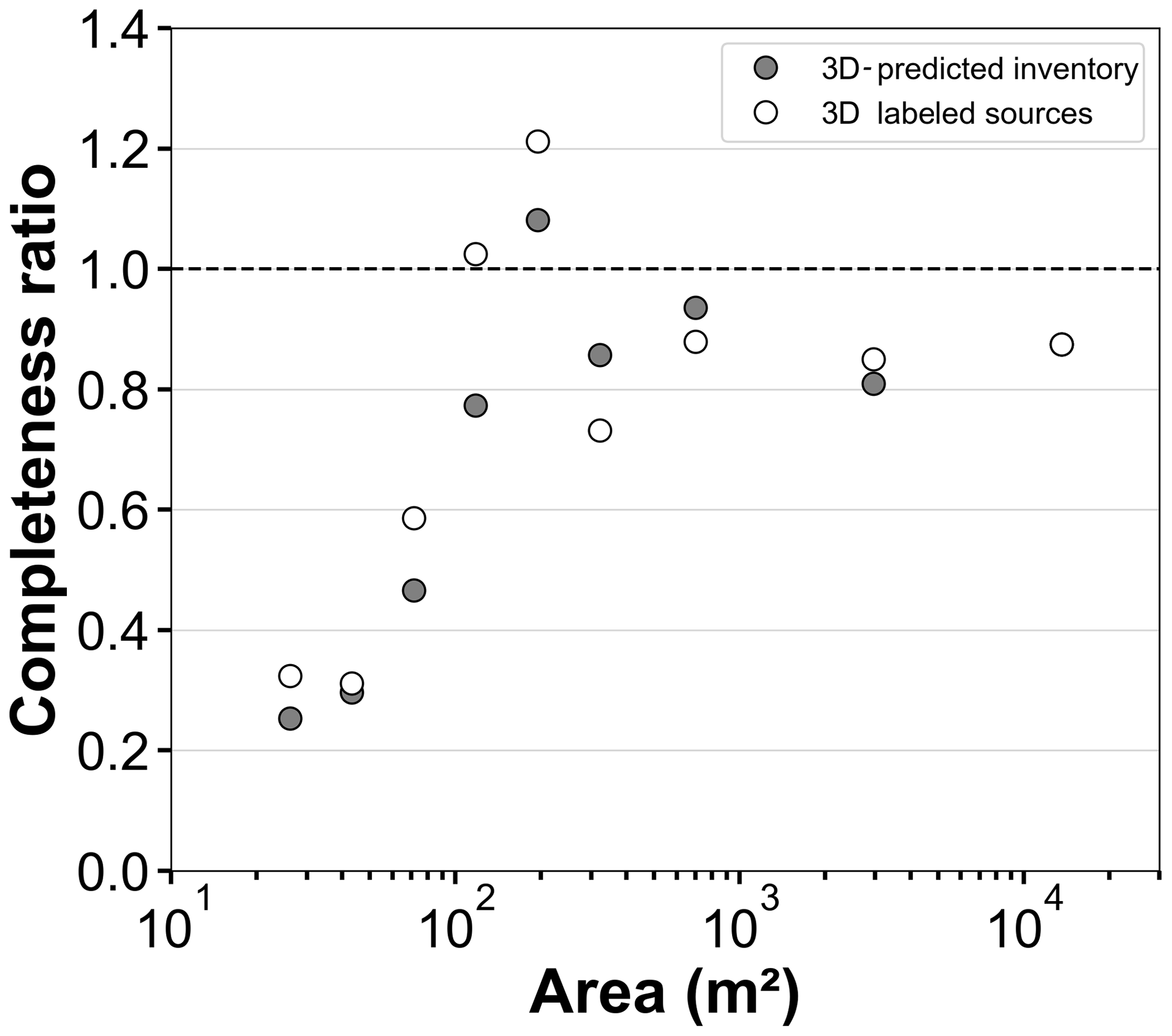
Figure 15Number of 2D corrected sources over number of 3D sources as a function of the source area. Assuming that the 3D inventory is nearly complete, this measure represents the ratio of completeness of the 2D inventory.
5.3.3 Distribution of landslide volume
Here, we present one of the first coseismic landslide volume distributions derived directly from 3D topographic data (Fig. 11b), rather than inferred from the combination of the landslide area distribution, based on 2D data, and an estimated V–A relationship. Our direct measurements show that the landslide volume distribution indeed obeys a power-law relationship for V > 50 m3 with an exponent e= −1.54 ± 0.07, consistent with the very broad range of exponents estimated in previous studies of −1.0 and −1.5 for rock and soil landslides, respectively (e.g., Brunetti et al., 2009; Malamud et al., 2004)). The sensitivity analysis to the workflow parameters (Fig. S7, Table S4) shows that the exponent e will decrease with reg, as this parameter will censor progressively thinner landslides which are statistically the smallest ones. Contrary to the distribution of source area, the segmentation distance Dm has little impact on e.
A deviation from the power-law trend occurs around 80 m3 with a rollover point around 20 m3, which is very close to the minimum volume that we can theoretically detect (∼ 8 m3). Thus, it is difficult to evaluate if the deviation is a real feature or an underdetection due to the lower depth limit that the 3D-PcD method can detect given the registration error (40 cm). Because no rollover is observed in p(A), our data may hint at a different landsliding process resulting in smaller depth for small landslides, but the D–A relationship is too scattered to detect a different trend. As we suspect that our inventory may contain a small fraction of very large rockfalls, the comparison with rockfall volume statistics is relevant. The probability distribution of rockfall volume generally obeys a power-law relationship with an exponent eR ranging from −1 to −2.2 (e.g., Malamud et al., 2004; Benjamin et al., 2020) without a rollover. If we restrict existing inventories to those with at least 500 rockfalls and the largest rockfall of at least of 20 m3, the range of exponent eR narrows to −1.5 to −2 with a majority of inventories around −1.6 ± 0.1 (Benjamin et al., 2020), which is very close to our scaling exponent. Although, we do not expect rockfalls to be a dominant mechanism in our database given the lack of very steep slopes and given that rupture mechanisms (e.g., fragmentation, sliding, slumping), rock heterogeneity and topographic constraints (e.g., hillslope size) are not expected to be similar (Dussauge et al., 2003), the consistency of the exponent that we find is striking. This may suggest a much larger range of scales over which the volume of landslides, encompassing rockfalls in this definition, obeys a unique scaling behavior. Datasets specifically acquired to bridge the gap between large-scale airborne lidar and terrestrial lidar are needed to get a better handle on the volume distribution of landslides, critical information with respect to risk analysis and landslide erosion calculation.
5.3.4 Landslide depth and volume–area relationship
Our 3D-PcD approach opens the possibility to directly quantify the variations in landslide depth with size. We show that landslide mean depth varies slightly with landslide area – on average by less than 1 order of magnitude for the given range of area of the 3D-predicted inventory. The same behavior has been observed by Larsen et al. (2010) for soil landslide scars, suggesting that our landslide inventory may be relevant to shallow landsliding. This is consistent with the fact that 50 % of the landslide thicknesses are lower than 1.6 m and that the landslide volume–area (V–A) scaling relationships obtained in this study are close to those of Massey et al. (2020) and Larsen et al. (2010) for soil landslides.
The sensitivity analyses to the workflow parameters show that the V–A exponent γ is not significantly affected by the variations in the reg values that we explored: γ varies from 1.17 ± 0.03 to 1.19 ± 0.03 (Fig. S8, Table S4). It is also not affected by the segmentation distance for Dm < 6 m, beyond which landslide amalgamation becomes significant and γ decreases to 1.1.
In this paper, we introduce a new workflow for semiautomated landslide source and deposit detection using 3D differencing based on high-resolution topographic point cloud data. This method uses the M3C2 algorithm developed by Lague et al. (2013) for accurate change detection based on the 3D distance normal to the local surface. Potential landslide sources and deposits are segmented using a 3D connected component approach, and their volumes are computed by a vertical-M3C2. Spatially variable uncertainties with respect to distance and volume are provided by the calculation and are used in the workflow to evaluate if a change is statistically significant or not, for volume uncertainty estimation and to define a confidence metric per source or deposit (SNR). Combined with the downslope distance to the closest deposit measured for each potential landslide source, the SNR is used to filter out false detections related to spatially correlated elevation errors such as intra-survey registration errors and ground classification errors in forests. We provide various tests and recipes to estimate the registration error and to choose the parameters of the M3C2 algorithm as functions of the point cloud density to ensure the lowest level of change detection as well as the best resolution of the 3D map of change. Applied to a 5 km2 area located in the Kaikōura region in New Zealand with pre- and post-earthquake lidar, we generate the first automatic inventory of landslide sources and deposits based on repeat 3D airborne lidar data. We show the following:
-
A minimum level of 3D change detection at 95 % confidence of 0.40 m can be reached with airborne lidar data, which is largely set by the registration error. In our case, the limited quality of flight-line alignment of the pre-EQ data was the dominant source of registration uncertainty. Because it operates on raw data, M3C2 accounts for characteristics such as point density and roughness that are not considered when working on DEMs, and it results in more robust statistics when it comes to evaluating if a change is significant or not. The 3D point cloud differencing method is critical for steep slopes and allows for a lower level of change detection compared with the traditional DoD.
-
Complex correlated elevation errors may result in long-wavelength low-amplitude false detections of landslide sources with a typical prevalence of 25 % in forest-free areas. They can be efficiently removed while preserving true landslides using a combination of the SNR and the newly introduced closest deposit distance (CDD). Landslide detection in the dense evergreen forest of our study area is more challenging owing to low ground point density and ground classification errors.
-
Considering 3D topographic change for landslide detection removes the amalgamation effect on the total landslide volume by directly measuring it in 3D rather than considering an ad hoc V–A relationship. Amalgamation in 3D is still an issue when exploring individual landslide area and volume statistics given the simplistic segmentation approach that we have used. However, our approach has the benefits of more systematically capturing small landslides than traditional approaches based on 2D imagery with manual landslide mapping.
-
Landslides on surfaces with small vegetation or no vegetation cover are classically missed with 2D imagery processing due to the lack of texture or spectral change. In our study case, 72 % of the landslide surface area is missed when considering a 2D inventory, corresponding to 54 % of the total volume determined with the 3D inventory. The landslide surface area is missed due to both detection error (landslide fully missed) and delimitation error (uncertainty with respect to outlines). Our method also shows the ability to detect subsidence related to slip failure propagation and the initiation or displacement of translational and rotational large landslides, which cannot be detected with 2D imagery.
-
As this method provides direct 3D measurement, landslide geometric properties such as volume, area, depth and their distributions can be explored. Our results are broadly consistent with the V–A relationship scaling parameters determined by Larsen et al. (2010) and Massey et al. (2020) for soil landslides, with a scaling exponent of 1.17.
-
No rollover is observed in the landslide area distribution down to 20 m2, which is our conservative resolution limit, using the 3D landslide inventory. However, we demonstrate, a size-based underdetection in landslides mapped from repeat 2D images, which in turn results in a cutoff of the power-law behavior of the 2D inventory and contributes to the rollover occurring at 20 m2. This result lends credit to the hypothesis that the rollover observed in landslide area distributions generated from 2D images is entirely or partially related to an underdetection of small landslides (Stark and Hovius, 2001).
Our 3D processing workflow is a first step towards harnessing the full potential of repeated 3D high-resolution topographic surveys to automatically create complete and accurate landslide inventories. However, high-density lidar flights are not always available in landslide-prone regions for which a 2D image-based approach remains the most suitable method. Nevertheless, we recommend systematically performing a 3D-PcD approach where repeat lidar data exist. This is critically needed to improve landslide science and manage the cascade of hazards following large earthquakes or storm events, by automatically identifying landslide deposits and subtle features such as subsidence developing around landslides missed in 2D inventories. Current bottlenecks to apply this workflow over larger scales, beyond the availability of high-quality 3D data, are the registration of pre- and post-EQ data when complex coseismic deformation patterns occur and the limitations of the segmentation method in high-landslide-density areas. While airborne lidar is best suited to vegetated environments and currently results in the best precision (compared with aerial or spatial photogrammetry), the workflow operates for any kind of 3D data.
The code used to produce the landslide inventory in this study is available as a Jupyter Notebook at https://github.com/Thomas-Brd/3D_landslide_detection (Bernard, 2021, https://doi.org/10.5281/zenodo.5220611, Bernard and Steer, 2021).
The landslide source and deposit information supporting the findings of this paper can be found at https://doi.org/10.5281/zenodo.5113770 (Bernard et al., 2021).
The supplement related to this article is available online at: https://doi.org/10.5194/esurf-9-1013-2021-supplement.
DL and TGB designed the landslide detection workflow. TGB, DL and PS all participated in the discussion, writing and reviewing of this paper. TGB produced the figures and the code. PS wrote the MATLAB-based code to calculate the CDD.
The authors declare that they have no conflict of interest.
Publisher's note: Copernicus Publications remains neutral with regard to jurisdictional claims in published maps and institutional affiliations.
We are grateful to Alex Densmore and David Milledge for the critical review that helped to improve this paper. We also wish to thank the editors, Giulia Sofia and Niel Hovius, for their time and feedback. Finally, we wish to acknowledge the European Reasearch Council, the Agence National de la Recherche, the Brittany region and the lidar topobathymetric platform of Rennes University for their financial support.
This research has been supported by the European Research Council, H2020 Research and Innovation program (grant no. FEASIBLe, 803721); the Agence Nationale de la Recherche (grant no. ANR-14-CE33-0005); and the LIDAREAU project, Brittany region (grant no. 2020-701).
This paper was edited by Giulia Sofia and reviewed by Alexander Densmore and Dave Milledge.
Aerial Surveys: Aerial photographs derived from two surveys of the study area carried out in 2014 to 2015 and in 2016 to 2017, Aerial Surveys Ltd, 2017.
Anderson, S. W.: Uncertainty in quantitative analyses of topographic change: error propagation and the role of thresholding, Earth Surf. Proc. Land., 44, 1015–1033, https://doi.org/10.1002/esp.4551, 2019.
Ankerst, M., Breunig, M. M., Kriegel, H.-P., and Sander, J.: OPTICS, ACM SIGMOD Rec., 28, 49–60, https://doi.org/10.1145/304181.304187, 1999.
Aryal, A., Brooks, B. A., Reid, M. E., Bawden, G. W., and Pawlak, G. R.: Displacement fields from point cloud data: Application of particle imaging velocimetry to landslide geodesy, J. Geophys. Res.-Earth, 117, 1–15, https://doi.org/10.1029/2011JF002161, 2012.
Barlow, J., Barisin, I., Rosser, N., Petley, D., Densmore, A., and Wright, T.: Seismically-induced mass movements and volumetric fluxes resulting from the 2010 Mw = 7.2 earthquake in the Sierra Cucapah, Mexico, Geomorphology, 230, 138–145, https://doi.org/10.1016/j.geomorph.2014.11.012, 2015.
Behling, R., Roessner, S., Kaufmann, H., and Kleinschmit, B.: Automated spatiotemporal landslide mapping over large areas using rapideye time series data, Remote Sens., 6, 8026–8055, https://doi.org/10.3390/rs6098026, 2014.
Behling, R., Roessner, S., Golovko, D., and Kleinschmit, B.: Derivation of long-term spatiotemporal landslide activity – A multi-sensor time series approach, Remote Sens. Environ., 186, 88–104, https://doi.org/10.1016/j.rse.2016.07.017, 2016.
Bellugi, D. G., Milledge, D. G., Cuffey, K. M., Dietrich, W. E., and Larsen, L. G.: Controls on the size distributions of shallow landslides, P. Natl. Acad. Sci. USA, 118, e2021855118, https://doi.org/10.1073/pnas.2021855118, 2021.
Benjamin, J., Rosser, N. J., and Brain, M. J.: Emergent characteristics of rockfall inventories captured at a regional scale, Earth Surf. Proc. Land., 45, 2773–2787, https://doi.org/10.1002/esp.4929, 2020.
Bernard, T. G.: 3D landslide detection, GitHub [code], available at: https://github.com/Thomas-Brd/3D_landslide_detection, last access: 19 August 2021.
Bernard, T. G. and Steer, P.: 3D landslide detection V2.0.0, Zenodo [code], https://doi.org/10.5281/zenodo.5220611, 2021.
Bernard, T. G., Lague, D., and Steer, P.: Landslide inventories from Bernard et al. (2021), Zenodo [data set], https://doi.org/10.5281/zenodo.5113770, 2021.
Besl, P. J. and McKay, N. D.: A Method for Registration of 3-D Shapes, IEEE T. Pattern Anal., 14, 239–256, https://doi.org/10.1109/34.121791, 1992.
Borradaile, G. J.: Statistics of earth science data: their distribution in space, time, and orientation, Springer-Verlag, New York, 2003.
Brardinoni, F. and Church, M.: Representing the landslide magnitude-frequency relation: Capilano River basin, British Columbia, Earth Surf. Proc. Land., 29, 115–124, https://doi.org/10.1002/esp.1029, 2004.
Brodersen, K. H., Ong, C. S., Stephan, K. E., and Buhmann, J. M.: The balanced accuracy and its posterior distribution, Proc. – Int. Conf. Pattern Recognit., 3121–3124, https://doi.org/10.1109/ICPR.2010.764, 2010.
Brodu, N. and Lague, D.: 3D terrestrial lidar data classification of complex natural scenes using a multi-scale dimensionality criterion: Applications in geomorphology, ISPRS J. Photogramm. Remote Sens., 68, 121–134, https://doi.org/10.1016/j.isprsjprs.2012.01.006, 2012.
Brunetti, M. T., Guzzetti, F., and Rossi, M.: Probability distributions of landslide volumes, Nonlin. Processes Geophys., 16, 179–188, https://doi.org/10.5194/npg-16-179-2009, 2009.
Bull, J. M., Miller, H., Gravley, D. M., Costello, D., Hikuroa, D. C. H., and Dix, J. K.: Assessing debris flows using LIDAR differencing: 18 May 2005 Matata event, New Zealand, Geomorphology, 124, 75–84, https://doi.org/10.1016/j.geomorph.2010.08.011, 2010.
Carrea, D., Abellan, A., Derron, M.-H., Gauvin, N. and Jaboyedoff, M.: MATLAB Virtual Toolbox for Retrospective Rockfall Source Detection and Volume Estimation Using 3D Point Clouds: A Case Study of a Subalpine Molasse Cliff, Geosciences, 11, 75, https://doi.org/10.3390/geosciences11020075, 2021.
Corsini, A., Borgatti, L., Cervi, F., Dahne, A., Ronchetti, F., and Sterzai, P.: Estimating mass-wasting processes in active earth slides – earth flows with time-series of High-Resolution DEMs from photogrammetry and airborne LiDAR, Nat. Hazards Earth Syst. Sci., 9, 433–439, https://doi.org/10.5194/nhess-9-433-2009, 2009.
Croissant, T., Lague, D., Davy, P., Davies, T., and Steer, P.: A precipiton-based approach to model hydro-sedimentary hazards induced by large sediment supplies in alluvial fans, Earth Surf. Proc. Land., 42, 2054–2067, https://doi.org/10.1002/esp.4171, 2017.
Crozier, M. J.: Landslides, in Environmental Geology, Kluwer Academic Publishers, Dordrecht, 371–375, 1999.
DiBiase, R. A. and Lamb, M. P.: Dry sediment loading of headwater channels fuels post-wildfire debris flows in bedrock landscapes, Geology, 48, 189–193, https://doi.org/10.1130/G46847.1, 2020.
Dolan, J. F.: Data Collection and Processing Report LiDAR survey of five fault segments (Eastern Clarence, Western Clarence, Central Eastern Awatere, West Wairau and East Hope-Conway) of the Marlborough Fault System on the Northwestern portion of New Zealand’s South Island, PhD, University of Southern California, Los Angeles, 11 pp., 2014.
Dussauge, C., Grasso, J.-R., and Helmstetter, A.: Statistical analysis of rockfall volume distributions: Implications for rockfall dynamics, J. Geophys. Res.-Sol. Ea., 108, 687–711, https://doi.org/10.1029/2001jb000650, 2003.
EDF R&D: Cloudcompare (version 2.12), available at: http://www.danielgm.net/cc/ (last access: 14 June 2021), 2011.
Esposito, G., Salvini, R., Matano, F., Sacchi, M., Danzi, M., Somma, R., and Troise, C.: Multitemporal monitoring of a coastal landslide through SfM-derived point cloud comparison, Photogramm. Rec., 32, 459–479, https://doi.org/10.1111/phor.12218, 2017.
Ester, M., Kriegel, H.-P., Sander, J., and Xu, X.: A Density-Based Algorithm for Discovering Clusters in Large Spatial Databases with Noise, in: Proceedings of the 2nd International Conference on Knowledge Discovery and Data Mining, 96, 226–231, 1996
Fairfield, J. and Leymarie, P.: Drainage networks from grid digital elevation models, Water Resour. Res., 27, 709–717, https://doi.org/10.1029/90WR02658, 1991.
Fan, Y., Clark, M., Lawrence, D. M., Swenson, S., Band, L. E., Brantley, S. L., Brooks, P. D., Dietrich, W. E., Flores, A., Grant, G., Kirchner, J. W., Mackay, D. S., McDonnell, J. J., Milly, P. C. D., Sullivan, P. L., Tague, C., Ajami, H., Chaney, N., Hartmann, A., Hazenberg, P., McNamara, J., Pelletier, J., Perket, J., Rouholahnejad-Freund, E., Wagener, T., Zeng, X., Beighley, E., Buzan, J., Huang, M., Livneh, B., Mohanty, B. P., Nijssen, B., Safeeq, M., Shen, C., van Verseveld, W., Volk, J., and Yamazaki, D.: Hillslope Hydrology in Global Change Research and Earth System Modeling, Water Resour. Res., 1737–1772, https://doi.org/10.1029/2018WR023903, 2019.
Frattini, P. and Crosta, G. B.: The role of material properties and landscape morphology on landslide size distributions, Earth Planet. Sc. Lett., 361, 310–319, https://doi.org/10.1016/j.epsl.2012.10.029, 2013.
Giordan, D., Allasia, P., Manconi, A., Baldo, M., Santangelo, M., Cardinali, M., Corazza, A., Albanese, V., Lollino, G., and Guzzetti, F.: Geomorphology Morphological and kinematic evolution of a large earth flow: The Montaguto landslide, southern Italy, Geomorphology, 187, 61–79, https://doi.org/10.1016/j.geomorph.2012.12.035, 2013.
Glennie, C.: Rigorous 3D error analysis of kinematic scanning LIDAR systems, J. Appl. Geod., 1, 147–157, https://doi.org/10.1515/jag.2007.017, 2008.
Glennie, C. L., Hinojosa-Corona, A., Nissen, E., Kusari, A., Oskin, M. E., Arrowsmith, J. R., and Borsa, A.: Optimization of legacy lidar data sets for measuring near-field earthquake displacements, Geophys. Res. Lett., 41, 3494–3501, https://doi.org/10.1002/2014GL059919, 2014.
Guzzetti, F., Malamud, B. D., Turcotte, D. L., and Reichenbach, P.: Power-law correlations of landslide areas in central Italy, Earth Planet. Sc. Lett., 195, 169–183, https://doi.org/10.1016/S0012-821X(01)00589-1, 2002.
Guzzetti, F., Mondini, A. C., Cardinali, M., Fiorucci, F., Santangelo, M., and Chang, K. T.: Landslide inventory maps: New tools for an old problem, Earth-Sci. Rev., 112, 42–66, https://doi.org/10.1016/j.earscirev.2012.02.001, 2012.
Hovius, N., Stark, C. P., and Allen, P. A.: Sediment flux from a mountain belt derived by landslide mapping, Geology, 25, 231, https://doi.org/10.1130/0091-7613(1997)025<0231:SFFAMB>2.3.CO;2, 1997.
Hungr, O., Leroueil, S., and Picarelli, L.: The Varnes classification of landslide types, an update, Landslides, 11, 167–194, https://doi.org/10.1007/s10346-013-0436-y, 2014.
Jeandet, L., Steer, P., Lague, D., and Davy, P.: Coulomb Mechanics and Relief Constraints Explain Landslide Size Distribution, Geophys. Res. Lett., 46, 4258–4266, https://doi.org/10.1029/2019GL082351, 2019.
Joerg, P. C., Morsdorf, F., and Zemp, M.: Uncertainty assessment of multi-temporal airborne laser scanning data: A case study on an Alpine glacier, Remote Sens. Environ., 127, 118–129, https://doi.org/10.1016/j.rse.2012.08.012, 2012.
Keefer, D. K.: The importance of earthquake-induced landslides to long-term slope erosion and slope-failure hazards in seismically active regions, Geomorphology, 10, 265–284, https://doi.org/10.1016/0169-555X(94)90021-3, 1994.
Kraus, K. and Pfeifer, N.: Determination of terrain models in wooded areas with airborne laser scanner data, ISPRS J. Photogramm. Remote Sens., 53, 193–203, https://doi.org/10.1016/S0924-2716(98)00009-4, 1998.
Lague, D., Brodu, N., and Leroux, J.: Accurate 3D comparison of complex topography with terrestrial laser scanner: Application to the Rangitikei canyon (N-Z), ISPRS J. Photogramm. Remote Sens., 82, 10–26, https://doi.org/10.1016/j.isprsjprs.2013.04.009, 2013.
Larsen, I. J., Montgomery, D. R., and Korup, O.: Landslide erosion controlled by hillslope material, Nat. Geosci., 3, 247–251, https://doi.org/10.1038/ngeo776, 2010.
Li, G., West, A. J., Densmore, A. L., Jin, Z., Parker, R. N., and Hilton, R. G.: Seismic mountain building: Landslides associated with the 2008 Wenchuan earthquake in the context of a generalized model for earthquake volume balance, Geochem. Geophy. Geosy., 15, 833–844, https://doi.org/10.1002/2013GC005067, 2014.
Lumia, R., Shapiro, L., and Zuniga, O.: A new connected components algorithm for virtual memory computers, Comput. Vision, Graph. Image Process., 22, 287–300, https://doi.org/10.1016/0734-189X(83)90071-3, 1983.
Malamud, B. D. and Turcotte, D. L.: Self-organized criticality applied to natural hazards, Nat. Hazards, 20, 93–116, https://doi.org/10.1023/A:1008014000515, 1999.
Malamud, B. D., Turcotte, D. L., Guzzetti, F., and Reichenbach, P.: Landslide inventories and their statistical properties, Earth Surf. Proc. Land., 29, 687–711, https://doi.org/10.1002/esp.1064, 2004.
Marc, O. and Hovius, N.: Amalgamation in landslide maps: effects and automatic detection, Nat. Hazards Earth Syst. Sci., 15, 723–733, https://doi.org/10.5194/nhess-15-723-2015, 2015.
Marc, O., Hovius, N., Meunier, P., Gorum, T., and Uchida, T.: A seismologically consistent expression for the total area and volume of earthquake-triggered landsliding – Marc – 2016, J. Geophys. Res.- Earth, 121, 640–663, https://doi.org/10.1002/2015JF003732, 2016.
Marc, O., Behling, R., Andermann, C., Turowski, J. M., Illien, L., Roessner, S., and Hovius, N.: Long-term erosion of the Nepal Himalayas by bedrock landsliding: the role of monsoons, earthquakes and giant landslides, Earth Surf. Dynam., 7, 107–128, https://doi.org/10.5194/esurf-7-107-2019, 2019.
Martha, T. R., Kerle, N., Jetten, V., van Westen, C. J., and Kumar, K. V.: Characterising spectral, spatial and morphometric properties of landslides for semi-automatic detection using object-oriented methods, Geomorphology, 116, 24–36, https://doi.org/10.1016/j.geomorph.2009.10.004, 2010.
Massey, C., Townsend, D., Rathje, E., Allstadt, K. E., Lukovic, B., Kaneko, Y., Bradley, B., Wartman, J., Jibson, R. W., Petley, D. N., Horspool, N., Hamling, I., Carey, J., Cox, S., Davidson, J., Dellow, S., Godt, J. W., Holden, C., Jones, K., Kaiser, A., Little, M., Lyndsell, B., McColl, S., Morgenstern, R., Rengers, F. K., Rhoades, D., Rosser, B., Strong, D., Singeisen, C., and Villeneuve, M.: Landslides triggered by the 14 November 2016 Mw 7.8 Kaikōura earthquake, New Zealand, B. Seismol. Soc. Am., 108, 1630–1648, https://doi.org/10.1785/0120170305, 2018.
Massey, C. I., Townsend, D., Jones, K., Lukovic, B., Rhoades, D., Morgenstern, R., Rosser, B., Ries, W., Howarth, J., Hamling, I., Petley, D., Clark, M., Wartman, J., Litchfield, N., and Olsen, M.: Volume Characteristics of Landslides Triggered by the MW 7.8 2016 Kaikōura Earthquake, New Zealand, Derived From Digital Surface Difference Modeling, J. Geophys. Res.-Earth, 125, e2019JF005163, https://doi.org/10.1029/2019JF005163, 2020.
McInnes, L., Healy, J., and Astels, S.: hdbscan: Hierarchical density based clustering, J. Open Source Softw., 2, 205, https://doi.org/10.21105/joss.00205, 2017.
Medwedeff, W. G., Clark, M. K., Zekkos, D., and West, A. J.: Characteristic landslide distributions: An investigation of landscape controls on landslide size, Earth Planet. Sc. Lett., 539, 116203, https://doi.org/10.1016/j.epsl.2020.116203, 2020.
Miller, D. J. and Burnett, K. M.: Effects of forest cover, topography, and sampling extent on the measured density of shallow, translational landslides, Water Resour. Res., 43, 1–23, https://doi.org/10.1029/2005WR004807, 2007.
Mora, O. E., Gabriela Lenzano, M., Toth, C. K., Grejner-Brzezinska, D. A., and Fayne, J. V.: Landslide change detection based on Multi-Temporal airborne LIDAR-derived DEMs, Geosciences, 8, 6–8, https://doi.org/10.3390/geosciences8010023, 2018.
Mouyen, M., Steer, P., Chang, K.-J., Le Moigne, N., Hwang, C., Hsieh, W.-C., Jeandet, L., Longuevergne, L., Cheng, C.-C., Boy, J.-P., and Masson, F.: Quantifying sediment mass redistribution from joint time-lapse gravimetry and photogrammetry surveys, Earth Surf. Dynam., 8, 555–577, https://doi.org/10.5194/esurf-8-555-2020, 2020.
Okyay, U., Telling, J., Glennie, C. L., and Dietrich, W. E.: Airborne lidar change detection: An overview of Earth sciences applications, Earth-Sci. Rev., 198, 102929, https://doi.org/10.1016/j.earscirev.2019.102929, 2019.
Parker, R. N., Densmore, A. L., Rosser, N. J., De Michele, M., Li, Y., Huang, R., Whadcoat, S., and Petley, D. N.: Mass wasting triggered by the 2008 Wenchuan earthquake is greater than orogenic growth, Nat. Geosci., 4, 449–452, https://doi.org/10.1038/ngeo1154, 2011.
Passalacqua, P., Belmont, P., Staley, D. M., Simley, J. D., Arrowsmith, J. R., Bode, C. A., Crosby, C., DeLong, S. B., Glenn, N. F., Kelly, S. A., Lague, D., Sangireddy, H., Schaffrath, K., Tarboton, D. G., Wasklewicz, T., and Wheaton, J. M.: Analyzing high resolution topography for advancing the understanding of mass and energy transfer through landscapes: A review, Earth-Sci. Rev., 148, 174–193, https://doi.org/10.1016/j.earscirev.2015.05.012, 2015.
Pollock, W. and Wartman, J.: Human Vulnerability to Landslides, GeoHealth, 4, 1–17, https://doi.org/10.1029/2020GH000287, 2020.
Pradhan, B., Jebur, M. N., Shafri, H. Z. M., and Tehrany, M. S.: Data fusion technique using wavelet transform and taguchi methods for automatic landslide detection from airborne laser scanning data and quickbird satellite imagery, IEEE T. Geosci. Remote, 54, 1610–1622, https://doi.org/10.1109/TGRS.2015.2484325, 2016.
Schwanghart, W. and Scherler, D.: Short Communication: TopoToolbox 2 – MATLAB-based software for topographic analysis and modeling in Earth surface sciences, Earth Surf. Dynam., 2, 1–7, https://doi.org/10.5194/esurf-2-1-2014, 2014.
Simonett, D. S.: Landslide distribution and earthquakes in the Bavani and Torricelli mountains, New Guinea, Cambridge Unviversity Press Cambrige, Landform S, 64–84, 1967.
Sithole, G. and Vosselman, G.: Experimental comparison of filter algorithms for bare-Earth extraction from airborne laser scanning point clouds, ISPRS J. Photogramm. Remote Sens., 59, 85–101, https://doi.org/10.1016/j.isprsjprs.2004.05.004, 2004.
Stark, C. P. and Guzzetti, F.: Landslide rupture and the probability distribution of mobilized debris volumes, J. Geophys. Res.-Earth, 114, 1–16, https://doi.org/10.1029/2008JF001008, 2009.
Stark, C. P. and Hovius, N.: The characterization of landslide size distributions, Geophys. Res. Lett., 28, 1091–1094, https://doi.org/10.1029/2000GL008527, 2001.
Stumpf, A., Malet, J. P., Allemand, P., Pierrot-Deseilligny, M., and Skupinski, G.: Ground-based multi-view photogrammetry for the monitoring of landslide deformation and erosion, Geomorphology, 231, 130–145, https://doi.org/10.1016/j.geomorph.2014.10.039, 2015.
Tanyaş, H., van Westen, C. J., Allstadt, K. E., and Jibson, R. W.: Factors controlling landslide frequency–area distributions, Earth Surf. Proc. Land., 44, 900–917, https://doi.org/10.1002/esp.4543, 2019.
Teza, G., Galgaro, A., Zaltron, N., and Genevois, R.: Terrestrial laser scanner to detect landslide displacement fields: A new approach, Int. J. Remote Sens., 28, 3425–3446, https://doi.org/10.1080/01431160601024234, 2007.
Tonini, M. and Abellan, A.: Rockfall detection from terrestrial lidar point clouds: A clustering approach using R, J. Spat. Inf. Sci., 8, 95–110, https://doi.org/10.5311/JOSIS.2014.8.123, 2014.
Ventura, G., Vilardo, G., Terranova, C., and Sessa, E. B.: Tracking and evolution of complex active landslides by multi-temporal airborne LiDAR data: The Montaguto landslide (Southern Italy), Remote Sens. Environ., 115, 3237–3248, https://doi.org/10.1016/j.rse.2011.07.007, 2011.
Wagner, W., Lague, D., Mohrig, D., Passalacqua, P., Shaw, J., and Moffett, K.: Elevation change and stability on a prograding delta, Geophys. Res. Lett., 44, 1786–1794, https://doi.org/10.1002/2016GL072070, 2017.
Wheaton, J. M., Brasington, J., Darby, S. E., and Sear, D. A.: Accounting for uncertainty in DEMs from repeat topographic surveys: Improved sediment budgets, Earth Surf. Proc. Land., 35, 136–156, https://doi.org/10.1002/esp.1886, 2010.
Williams, J. G., Rosser, N. J., Hardy, R. J., Brain, M. J., and Afana, A. A.: Optimising 4-D surface change detection: an approach for capturing rockfall magnitude–frequency, Earth Surf. Dynam., 6, 101–119, https://doi.org/10.5194/esurf-6-101-2018, 2018.
Zhong, C., Liu, Y., Gao, P., Chen, W., Li, H., Hou, Y., Nuremanguli, T., and Ma, H.: Landslide mapping with remote sensing: challenges and opportunities, Int. J. Remote Sens., 41, 1555–1581, https://doi.org/10.1080/01431161.2019.1672904, 2020.