Locating rock slope failures along highways and understanding their physical processes using seismic signals

Regional monitoring of rock slope failures using the seismic technique is rarely undertaken due to significant source location errors; this method also still lacks the signal features needed to understand events of this type because of the complex mass movement involved. To better comprehend these types of events, 10 known events along highways in Taiwan were analyzed. First, a hybrid method (GeoLoc) composed of cross-correlation-based and amplitude-attenuation-based approaches was applied, and it produced a maximum location error of 3.19 km for the 10 events. We then analyzed the ratio of local magnitude (M_L) and duration magnitude (M_D) and found that a threshold of 0.85 yields successful classification between rock slope failure and earthquake. Further, GeoLoc can retrieve the seismic parameters, such as signal amplitude at the source (A₀) and M_L of events, which are crucial for constructing scaling law with source volume (V). Indeed, Log(V) = 1.12 M_L + 3.08 and V = 77 290 $A_{\mathrm{0}}^{\mathrm{0.44}}$ derived in this study provide the lower bound of volume estimation, as the seismic parameters based on peak amplitudes cannot represent the full process of mass loss. Second, while video records correspond to seismic signals, the processes of toppling and sliding present column- and V-shaped spectrograms, respectively. The impacts of rockfall link directly to the pulses of seismic signals. Here, all spectrogram features of events can be identified for events with volumes larger than 2000 m³, corresponding to the farthest epicenter distance of ∼ 2.5 km. These results were obtained using the GeoLoc scheme for providing the government with rapid reports for reference. Finally, a recent event on 12 June 2020 was used to examine the GeoLoc scheme's feasibility. We estimated the event's volume using two scalings: 3838 and 3019 m³. These values were roughly consistent with the volume estimation of 5142 m³ from the digital elevation model. The physical processes, including rockfall, toppling, and complex motion behaviors of rock interacting with slope inferred from the spectrogram features were comprehensively supported by the video record and field investigation. We also demonstrated that the GeoLoc scheme, which has been implemented in Sinwulyu catchment, Taiwan, can provide fast reports, including the location, volume, and physical process of events, to the public soon after they occur.

1 Introduction

Failures caused by the instability of rock mass are the most common geohazard in mountainous terrain. For this type of mass movement, rock instability can refer to the falling, toppling, slumping, sliding, spreading, creeping, or avalanche of the mass block (Varnes, 1978). A lack of direct observations in the field leads to a challenge in determining the type of mass movement. In general, a rockfall involves physical processes, such as detachment, falling, rolling, bouncing, and fragmentation. It mainly interacts with the substrate, not necessarily with other moving fragments. A rockslide is usually due to instability along a bedding plane or a discontinuous, weakened structure, and failure is often associated with a complex mechanism. A rock topple is forward rotation and overturning of the rock body (Hungr et al., 2013). Here, we use the term “rock slope failure” (RSF) to represent the aforementioned terms, including rockfall, rockslide, and rock topple along the highways, which can potentially cause damage to humans and the environment.

RSFs that occur along the highways may threaten road users and damage the road and facilities. Thus, it is essential to get precise information about the timing, location, and moving volume of such events within a short time for the purpose of issuing warnings and understanding the physical process of failures for the assessment of hazard management, field survey, and slope protection after events. Recently, the seismic technique has been widely used for those purposes for RSF events, not only at a local scale (Vilajosana et al., 2008; Helmstetter and Garambois, 2010; Zimmer et al., 2012; Zimmer and Sitar, 2015; Dietze et al., 2017; Le Roy et al., 2019) but also at a regional scale (Dammeier et al., 2011; Manconi et al., 2016; Fuchs et al., 2018). In the case of a free-fall event, the leading seismic signals corresponding to crack propagation and rock impact occupy a higher-frequency band than the signals induced by rock detachment and rebound (Levy et al., 2011; Dietze et al., 2017; Le Roy et al., 2019). A series of field-scale block rockfall experiments were conducted to generate signal templates related to the rolling, bouncing, and impacting of a single block mass, with their respective pulse features shown in the time–frequency spectrograms. During rock fall, the mass particle might be fragmented, and the individual particles not only interact with the topographic surface but also collide with each other (Hilbert et al., 2017; Saló et al., 2018). Based on a combined analysis of the seismic signals and high-speed video cameras, Saló et al. (2018) found that the impact of large rock boulders on a slope can generate lower-frequency seismic signals than the impact corresponding to the process with fragmented blocks. Then, for the sliding phase, Manconi et al. (2016) indicated that the spectrograms induced by sliding-controlled behavior exhibit the traditional triangular shape, which is the same feature as that of landslides (Chen et al., 2013; Hibert et al., 2014) and snow avalanches (Suriñach et al., 2005). Recent studies also concluded that massive, rapid landslides, which include the processes of acceleration and deceleration, could generate strong long-period (10–150 s) seismic signals (Ekström and Stark, 2013; Chao et al., 2017). By contrast, the on-site seismic signals of RSFs with frequencies up to 50–100 Hz would be very helpful in exploring the source dynamics. However, most of the studies based on regional seismic networks focused on lower frequencies ranging from 0.1 to 20 Hz due to the attenuation effect of wave propagation (Deparis et al., 2008; Dammeier et al., 2011; Manconi et al., 2016; Fuchs et al., 2018), resulting in an imperfect understanding of the physical process of RSF.

Some studies have proposed a fully automatic scheme for locating and estimating the size of landslides (Chao et al., 2017), rockslides (Manconi et al., 2016; Fuchs et al., 2018), lahar (Kumagai et al., 2009), and debris flows (Walter et al., 2017) for rapid response purposes. At present, there are two main approaches to scanning the location of an RSF: the cross-correlation (CC) method and the amplitude source location (ASL) method. CC has been applied to sources with unclear phases in seismic arrivals, but this technique is susceptible to the regional velocity model, station coverage, and signal-to-noise ratio (SNR) of observed signals (Chen et al., 2013; Hibert et al., 2014), which are factors that influence location error. In contrast to CC, ASL does not require a priori knowledge of the velocity structure with inversion way and can estimate not only the source location but also the seismic parameters, such as the anelastic attenuation of seismic waves (α) and seismic amplitude at the source (A₀) (Aki and Ferrazzini, 2000; Jones et al., 2013; Röösli et al., 2014; Ogiso and Yomogida, 2015; Walter et al., 2017). However, ASL significantly relies not only on large bursts of seismic amplitude, which are influenced by the site conditions, but also on the distribution of the epicenter distance between each station and the source.

Figure 1 The research area and distribution of seismic stations and 10 rock slope failures (RSFs, yellow stars): (a) topographic map of Taiwan showing the three provincial highways (red lines) and BATS/CWB stations (blue squares); (b) Liwu catchment, the east flank of the central provincial highway, and the temporary seismic network (L-NET, pink squares); (c) Sinwulyu catchment, the east flank of the southern provincial highway, and the temporary seismic network (S-NET, pink squares). The data of the digital terrain model (DTM) of Taiwan and two catchments are from the Government Open Data Platform, Taiwan.

In this study, we develop the GeoLoc scheme which can determine the location of a geohazard, classify the source type, estimate the event volume (V), and may offer information about the physical process of RSF events. Thus, the information yielded by the GeoLoc scheme may make rapid reports to the government possible. The method of location determination also uses GeoLoc by combining the CC and ASL techniques with horizontal and vertical seismic signals. In this case, 10 RSFs with volumes ranging from 108 to 164 000 m³ that occurred along highways (see Table S1 and Sect. S1 in the Supplement) and were documented by the Directorate General of Highways (DGH) in Taiwan are used to explore the feasibility of GeoLoc. Further, the retrieved seismic parameters, A₀ from ASL and local magnitude (M_L) are used with event volume to build regressions for volume estimation. Recently, a simple scaling between the source magnitude and volume has been well established, covering a wide range of source volumes from 10⁰ to 10⁶ m³. However, there is a scatter trend in the data distribution for volumes ranging from 10² to 10⁵ m³ (Le Roy et al., 2019), which is shown in this research. Moreover, with available videos published on public platforms (Table S2 in the Supplement), we demonstrated that important physical processes related to seismic signals could be clarified – when the farthest epicentral distance is less than 2.5 km from events of at least 2000 m³. After the successful feasibility test of 10 events, a recent RSF event that occurred on 12 June 2020 was used to underscore the implications of the potential use of this rapid reporting system of RSF events that occur on slopes near highways.

2 Background setting and seismic data

Taiwan is located at the boundary of the Eurasian Plate and the Philippine Sea Plate (Fig. 1a), resulting in complex tectonic structures and high seismicity. The combined effect of extreme climate-forced erosion and strong earthquake shaking frequently causes RSF events. Vehicular traffic along three provincial highways, which cross the island of Taiwan from east to west, suffers from the potential threat of RSFs, especially at Taroko National Park along the east flank of the central cross-island highway, which attracts more than 4 million tourists every year. Thus, a rapid RSF report system is sorely needed for the safety of highway travelers. In practice, after RSFs occur on highways, the materials blocking the road are cleared and unmanned aerial vehicle (UAV) surveys are routinely performed by DGH. Some events can be captured by video and/or recorded by eyewitnesses. The above information allows us to obtain preliminary data about an RSF, such as the location, occurrence time, volume, and its physical process. Additionally, the Broadband Array in Taiwan for Seismology (BATS) seismic network, maintained by the Institute of Earth Sciences of Academia Sinica (IESAS) (Kao et al., 1998) and the Central Weather Bureau (CWB), is well distributed throughout Taiwan and provides high-quality seismic records for studying RSFs. The present broadband seismic network provides an opportunity to monitor RSFs. However, the primary purpose of this network is to monitor earthquakes. To enhance the station coverage along the highways for the high-risk areas (Crespi et al., 1996; Petley, 1998), temporal seismic arrays have been set up since March 2015 in Liwu catchment (shown as L-NET in Fig. 1b), consisting of one broadband seismometer (Güralp CMG-6TD; LW01 station) and four short-period sensors (Kinkei KVS-300; stations LW02-LW05), and in Sinwulyu catchment (shown as S-NET in Fig. 1c), consisting of seven broadband seismic stations (Nanometrics Trillium Compact: CLAB, DLNB, WLUB and XAMB; Güralp CMG-6TD: SW01-SW03). Thus, a total of 13 BATS/CWB broadband stations and 12 temporal stations are used in this study.

Figure 2 Flowchart of the GeoLoc scheme, including data preprocessing, location process, source classification, and volume estimation. All steps are automatic except the steps with gray shading, which involved a manual check in this research. f_L and f_H are the respective lower and upper band of the band-pass filtering. $(X,Y{)}_{\text{ASL/CC}-\text{H/Z}}$ is the best location from the ASL or CC with horizontal or vertical components. ($\mathit{\sigma }X,\mathit{\sigma }Y{)}_{\text{ASL/CC}-\text{H/Z}}$ are those location uncertainties based on the relative fitness over 0.95. N is the number of results from methods with components (total: N = 4) whose location error is less than the 5 km threshold. The result with the minimum location error defines the best location.

3 Flowchart of the GeoLoc scheme

This research presents a flowchart showing the specific steps involved in a near-automatic scheme (GeoLoc). The GeoLoc scheme consists of a four-step automatic procedure: (1) data preprocessing, (2) location process, (3) source classification, and (4) volume estimation (dashed rectangles in Fig. 2). However, manual time–frequency analysis is necessary to extract the frequency band of band-pass filtering, the signal duration, and the physical process. The first of the two procedures are addressed in Sects. 3.1 and 3.2, respectively. Once the best location of the source is determined, the classification of the source type is required. We analyzed the ratio of local magnitude and duration magnitude (M_L/M_D) for the source classification and established scaling laws of V, M_L, and A₀ to estimate the event volume for the detected RSF event (see Sect. 4.2). The current GeoLoc scheme does not involve analyzing the physical process in automatic implementation (see Sect. 4.3). However, the optional time–frequency analysis could provide an event's physical process based on the spectrogram features, such as V-shaped, column-shaped, and pulse-like patterns. The GeoLoc scheme can be operated as a partly automatic monitoring system that delivers rapid reports providing the best source location and volume of the event to the road users and government for RSF hazard assessment and mitigation. Comprehensive details are given in the following sections.

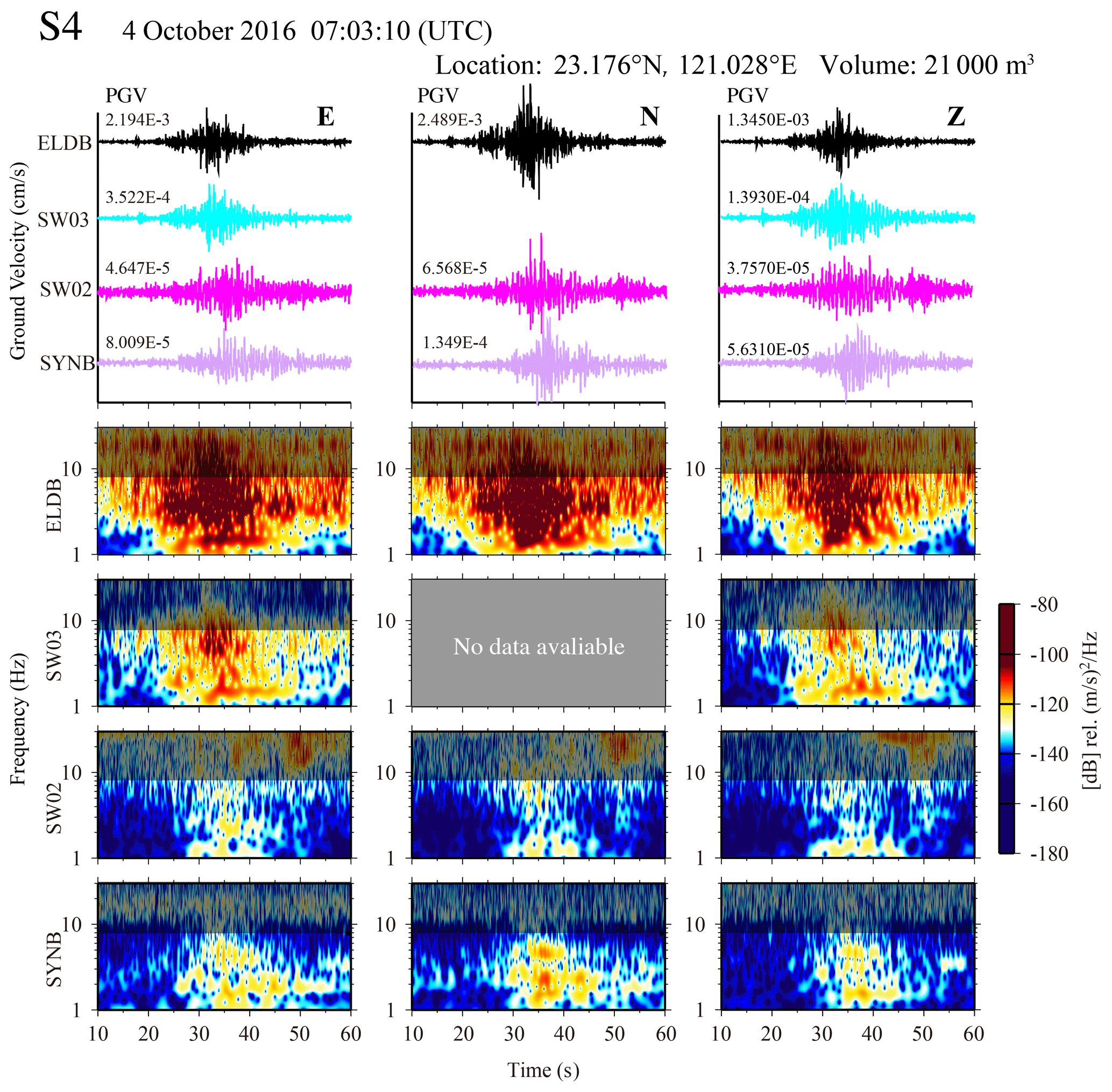
Figure 3 Recorded waveform and spectrogram of Event S4. The value next to the waveform is the peak ground velocity (PGV) for each signal. The bright area of the spectrogram is the range of the band-pass filter (1–8 Hz, f_L to f_H), which should cover the signals of all stations recorded during the event.

3.1 Data preprocessing

Based on the occurrence time and location of RSFs documented by the DGH, the three-component seismic recordings from nearby stations with a 180 s length window can be cut and then undergo preprocessing, including removing the mean and linear trend. Further, the time–frequency spectrograms are constructed. In the present study, a filtering range is selected that can effectively explain the strong power spectral density (PSD) distributed in the time–frequency map of all stations. A series of spectrogram analyses utilizes the S-transform (Chen et al., 2013). Figure 3 shows an example of the determination of the filtering range for Event S4. The spectrogram of ELDB station shows a strong PSD with a wide frequency range of 1–30 Hz. In contrast, the PSD distribution of SYNB station is contained at frequencies below 8 Hz, while the high-frequency signals should decay due to the attenuation of seismic wave propagation. Indeed, cutoff frequencies of 1–8 Hz which fit to all stations recording Event S4 are used in the band-pass filter. Other events inherit their filtering range the same way and are shown in Figs. S1–S4 in the Supplement. We then compute the root-mean-square (RMS) amplitudes of the filtered horizontal (N–S and E–W) and vertical waveforms and extract the horizontal and vertical envelope functions from the filtered RMS waveforms. Only when envelope functions have an SNR higher than 1.5, and the detected station number is over two, is the GeoLoc location process is considered. The SNR is calculated from the ratio between short-term and whole-term (180 s in time length) averages. The short-term average is the average value of a ± 5 s time window whose center is the peak envelope amplitude.

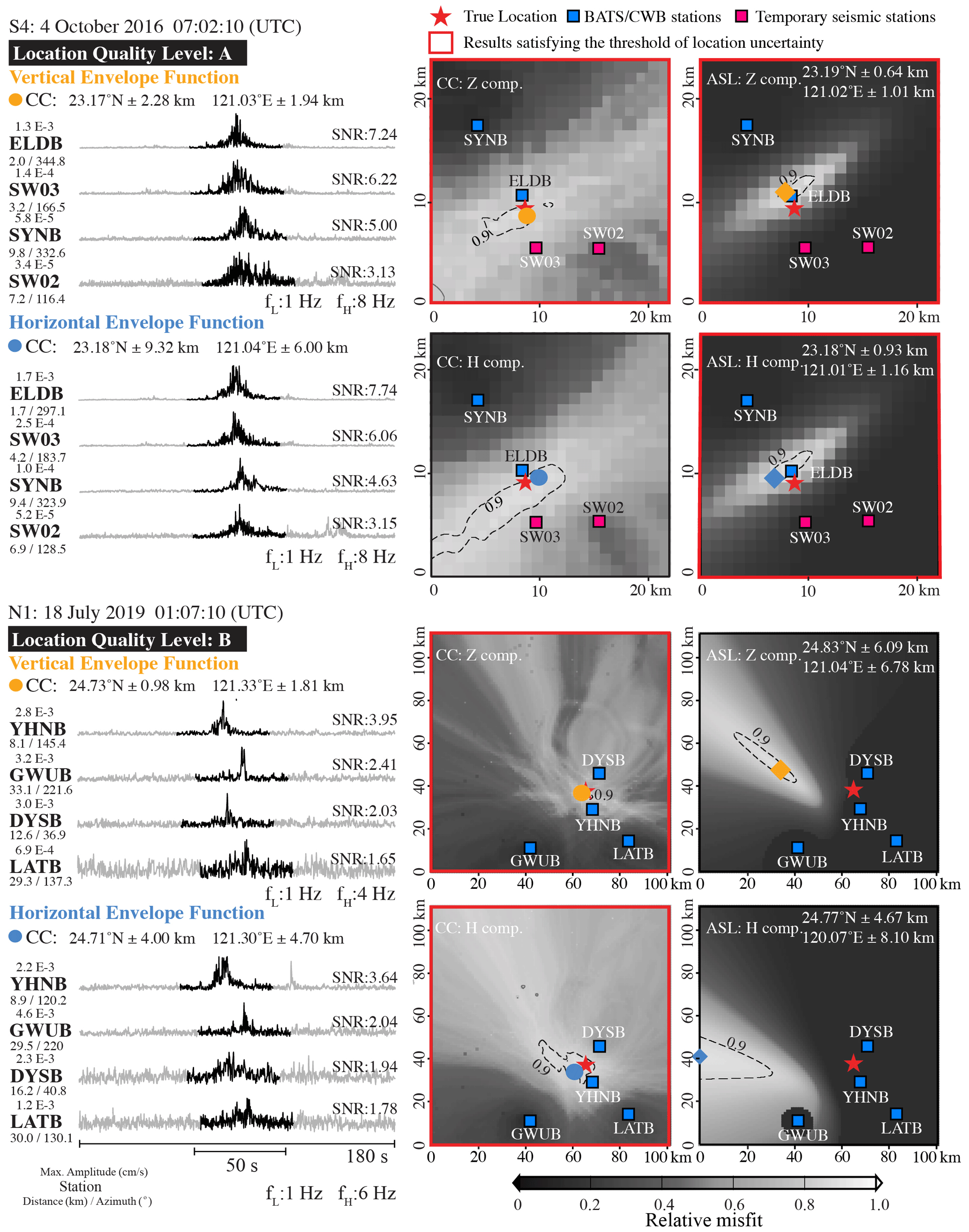
Figure 4 The result of CC and ASL in events S4 and N1. The left panel is the horizontal and vertical envelope function of the detected stations for events S4 and N1. The black lines with 50 s signals are used in the CC. The right panel is the result of the CC and ASL with a horizontal and vertical component. The circle and diamond symbols present the best result of the CC and ASL, respectively. The black dashed lines are the contour of a relative misfit of 0.9. The uncertainty of the location is estimated based on the standard deviation of longitude and latitude for the source grid points with a relative misfit higher than 0.95.

3.2 Location process

In the GeoLoc location process, events are detected by at least two stations with signal-to-noise ratios (SNRs) exceeding 1.5 in the envelope functions. GeoLoc combines the cross-correlation (CC) method (Chen et al., 2013) and the amplitude source location (ASL) method (Walter et al., 2017) using the vertical and horizontal envelope functions for source location determination. The ASL technique not only locates the event but also provides the seismic parameters of the signal amplitude at the source (A₀) and signal decay constant (α) based on the best fit of the amplitude decay curve by using a least squares scheme, which represents the peak amplitude at ith station (A_i) decay with increasing source-to-station distance (r_i) (Eq. 1). This ASL approach is available only when the epicentral distance is well distributed for a large number of stations. On the other hand, the CC approach relies on each station pair's waveform similarity. For each station pair of vertical and horizontal envelope function, the maximum normalized cross-correlation coefficient was calculated and the source location could be found by minimizing the cross-correlation amplitude misfit with each searching grid. Details on the CC method can be found in Chen et al. (2013). However, the CC approach needs a velocity model to compute the theoretical travel-time difference between two stations. In contrast, ASL does not require prior knowledge of the velocity structure. Compared with ASL, the CC method only produces an event location. A three-dimensional velocity model of Wu et al. (2007) is adopted in this study. A ± 25 s time window is used for the location process, and its center is the peak envelope amplitude (black traces shown in Fig. 4). A grid point on the free surface topography with 0.01^∘ spacing is established for the location search. For the ASL method, we assume surface waves are the dominant seismic wave type induced by RSFs (Dietze et al., 2017), so an n value in Eq. (1) of 0.5 (n = 1 for body waves and n = 0.5 for surface waves) is used to account for the amplitude attenuation due to geometrical spreading. Thus, there are only two unknown parameters of A₀ and α in Eq. (1).

$$\begin{array}{}\text{(1)}& A_i\left(r\right)={\displaystyle \frac{A_{\mathrm{0}}}{r_i^n}}{e}^{-\mathit{\alpha }{r}_i}\end{array}$$

The GeoLoc scheme was applied to determine the CC location (X_CC, Y_CC) and the ASL location (X_ASL, Y_ASL) simultaneously by minimizing the misfit functions for events. The misfit functions used in ASL and CC approaches are calculated from discrepancies in the peak envelope amplitude and cross-correlation amplitude, respectively. The relative fitness value is then defined by the normalized misfit functions with ranges from 0 to 1. We then compute the uncertainties (σX_ASL/CC, σY_ASL/CC) of location results using the standard deviation of longitude and latitude for the source grid points with the relative fitness value higher than 0.95. Then, the location result of the grid point with the highest relative fitness is chosen as the best solution. To understand the relationship between location uncertainty and location error, it is necessary to find the location error between the true location and the resulting source location. We found that the resulting locations with uncertainties (σX and σY) less than 5 km exhibit small location error (< 3.19 km). Thus, a threshold of location uncertainty of 5 km is used, and only location results satisfying this threshold are available and discussed later in the next section. For an event, the combination of two methods (CC and ASL) and two envelope functions (horizontal and vertical) can offer four location results, so the total amount of available result location (N) is four. We characterize the quality of a solution for the RSF event based on the N value. The quality level labels are A: 3≤N; B: 1≤N < 3; and C: N = 0. The best source location result for each RSF is determined by the minimum uncertainties from N of the available result locations. In Event S4, the three results' locations satisfy the uncertainty threshold (red frame in Fig. 4), so the location quality is A. The best source location result is then produced by the ASL with a vertical envelope. For Event N1, N equals 2 and belongs to the quality level B. The best location is the output of the CC with a horizontal envelope.

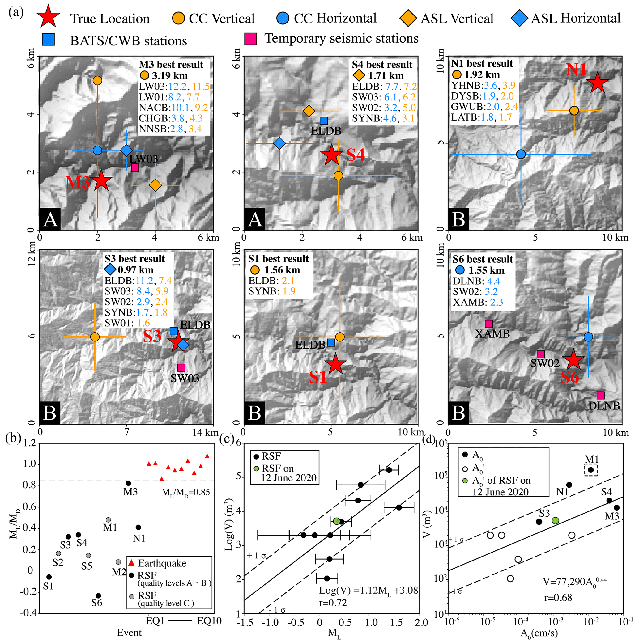
Figure 5 Results of the location process by the GeoLoc scheme, $M_{\mathrm{L}}/M_{\mathrm{D}}$ of the RSFs and earthquakes, scaling of seismic parameters, and source volumes. (a) Results of location quality levels A and B from GeoLoc and their location uncertainties. The numbers beside the station names shown in the top-right corner are the SNR values for the horizontal (blue) and vertical (orange) envelopes. The symbol in the white box is the best location result, and the value beside the symbol indicates the location error. (b) $M_{\mathrm{L}}/M_{\mathrm{D}}$ of RSFs and earthquakes; a horizontal dashed line indicates the $M_{\mathrm{L}}/M_{\mathrm{D}}$ threshold of 0.85 used in this study. The relationships of (c) the event volume (V) and M_L and (d) the event volume (V) and A₀. The black circles show the A₀ extracted from the best location result. The open circles are the peak ground velocity ($A_{\mathrm{0}}^{\prime }$), extracted from the nearest stations. Event M1 is excluded from the regression analysis due to its high location error. The data of the digital terrain model (DTM) of Taiwan are from the Government Open Data Platform, Taiwan.

4 Results and discussion

4.1 Location

After analyzing 10 RSFs along highways, the events with quality levels A (events S4 and M3) and B (events S1, S3, S6, and N1) that occurred during the non-typhoon period were determined with location errors between 0.97 and 3.19 km (Fig. 5a). The volume of these events is higher than 2000 m³ (Table S1). A small event size and a high background noise level, which result in poor waveform quality, causing the location quality level C, are two significant factors contributing to location error. For example, the two smallest events with a volume of 108 m³ (Event S5) and 400 m³ (Event M2) exhibit a high location error of 3.76 and 44.14 km, respectively. Even though Event M1 is the largest event, it can lead to a large location error of 23.61 km because of the high background noise level during the typhoon period with a low SNR value at each station (Table S1).

A hybrid GeoLoc provides a functional event location for the different station coverage conditions and the distribution of epicentral distances. In general, the CC method mainly relies on station coverage. Thus, Event S4 shows that location uncertainty has a clear trend along the station gap, existing in the northeast-to-southwest direction. However, there is a relative lack of influence on the result derived from the ASL method (Fig. 4). On the contrary, Event N1, with proper station coverage, still leads to a high location uncertainty in the ASL case which underscores that a well-distributed epicentral distance is a crucial factor for the ASL method. A previous study also demonstrated that the site amplification could strongly influence the location result (Walsh et al., 2017). At a local-scale area, site amplification factors for the specific station can be estimated easily by the ratios of coda amplitudes relative to a reference station (Kumagai et al., 2009). However, the aim of this study is to propose a rapid system to provide information about the timing, location, and moving volume of such events within a short time to the highway authority. For the seismic stations along highways, it is difficult to select a reference station, which will be a challenge to comprehensively investigate the site amplification based on the method adopted in Kumagai et al. (2009). In Taiwan, recent studies (Lai et al., 2016; Kuo et al., 2018) on the site amplification for the existed seismic network have been accumulated. The site effect of our station can be corrected, and this will need to be done in our future studies.

4.2 Source discrimination and volume estimation

For rapid RSF hazard assessment along roads, successful source classification and event size estimation are needed. Manconi et al. (2016) proposed that the ratio between the local magnitude (M_L) and the duration magnitude (M_D) ($M_{\mathrm{L}}/M_D$ = 0.8) could effectively distinguish a rockslide event from earthquake sources. To further examine the threshold of $M_{\mathrm{L}}/M_{\mathrm{D}}$ in our case, we selected 10 local earthquakes from the CWB catalogue (Table S3 in the Supplement) and collected seismic records of earthquakes from BATS and S-NET stations. We applied the same analysis procedures as in the RSF event, and all earthquakes analyses resulted in location quality levels of A or B. For both earthquakes and RSFs, the magnitude scales of M_L and M_D for the best location are computed, and the ratio of $M_{\mathrm{L}}/M_{\mathrm{D}}$ is then derived (see Sect. S3 in the Supplement). In the case of the earthquakes, the average $M_{\mathrm{L}}/M_{\mathrm{D}}$ ratio is 0.98, with a minimum value of 0.86. For the RSFs, $M_{\mathrm{L}}/M_{\mathrm{D}}$ ratios are 0.24 on average, and they never exceed 0.82. Thus, the threshold of $M_{\mathrm{L}}/M_{\mathrm{D}}$ of 0.85 is used to distinguish RSFs and earthquakes (Fig. 5b). We also found that the relationship between M_L and M_D in local earthquakes is consistent with the regression line derived in Shin (1993) (see Sects. S3 and S5 in the Supplement).

To mitigate the hazards caused by RSFs, rapid determination of source volume is essential for making emergency responses. We first build an empirical relation of Log(V) = 1.12 M_L + 3.08, as shown in Fig. 5c. The ASL method in the GeoLoc location process can provide the seismic amplitude at the event source (A₀), which is an additional parameter in estimating event size. Before exploring the relationship between V and A₀, a test was conducted to investigate the influence of location uncertainty on the A₀ value. After making the amplitude correction of A₀ for the specific events (see Sect. S4 in the Supplement), we further established a simple power scaling of V = 77 290 $A_{\mathrm{0}}^{\mathrm{0.44}}$ with a linear correlation coefficient (R) of 0.68 (Fig. 5c) and A₀ ranging from 1.60 × 10⁻⁵ to 6.61 × 10⁻² cm s⁻¹ (Table S1). However, the volume estimate from the two scalings could be underestimated because both M_L and A₀ were derived based on the peak amplitude. We expected that M_L and A₀ were sensitive to the moment of the highest energy release, such as the most significant boulder impact from a sequence of rockfalls or the rock mass impact on the slope/road from the toppling event, which cannot represent the entire process. Thus, the estimation from M_L−V and A₀−V offer the lower bound for total volume loss.

Another parameter α is linked to the seismic energy lost due to attenuation along with wave propagation. We collected the α values from three events (Table S4 in the Supplement), where their ASL results yielded the location uncertainty threshold. The result indicates that the attenuation is more rapid in the Sinwulyu catchment than in the Liwu catchment due to the geological background (see Sect. S4 in the Supplement).

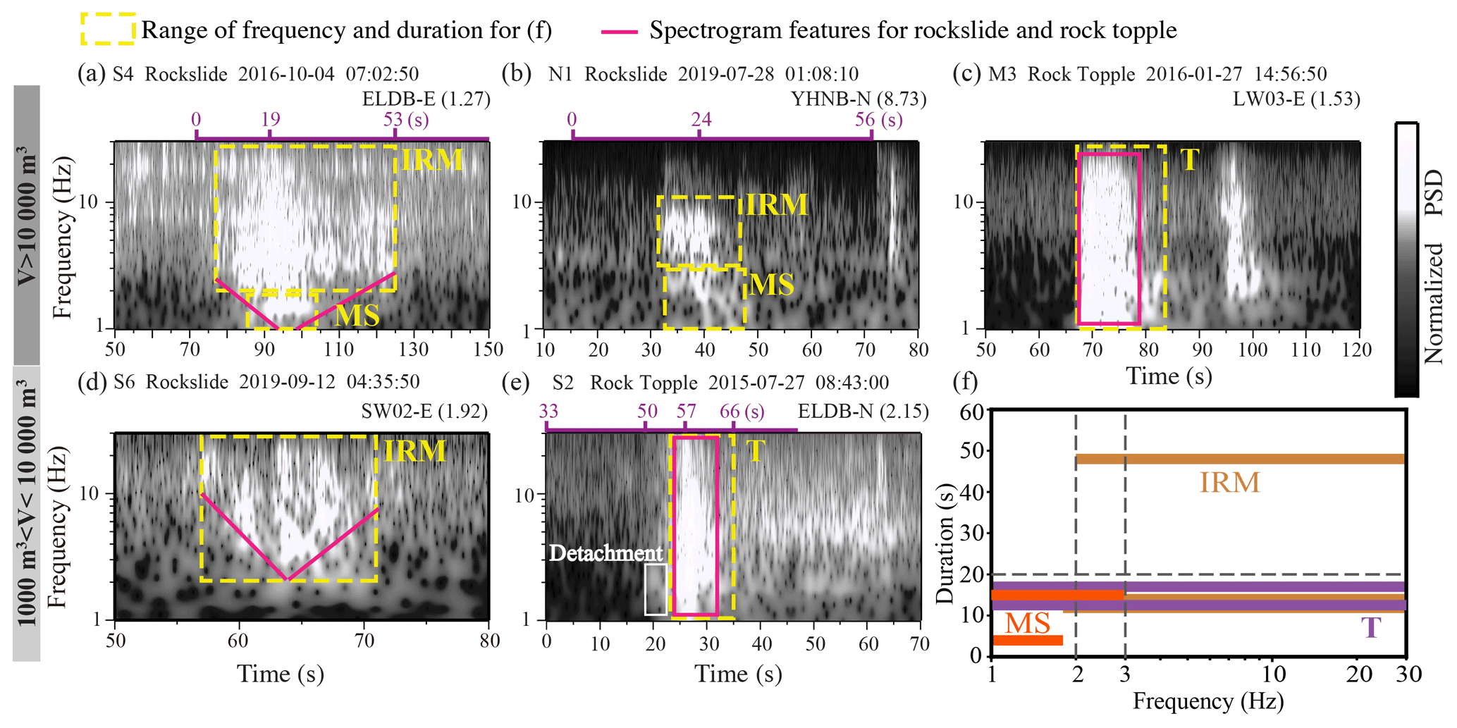
Figure 6 Spectrogram of five events and the classification of physical processes by spectrogram features, frequency, and duration. The rows are separated for the different scales of failure volumes. (a–e) Spectrograms of different events. The panel headings show the event number, the physical process, and the starting time of the x axis. The text in the top right displays the station name with the component and the epicentral distance (km). The purple bars above panels (a), (b), and (e) are the durations (in seconds) of the video with the time points (Table S2). (f) Sliding and toppling processes are distinguished by the frequency and event duration.

4.3 Physical process

Most of the RSFs were recorded by cameras and/or documented by news reports (Table S2), which provided an advanced understanding of the relation between the physical processes and the associated seismic signals. Based on events with a comprehensive video of the above observations, we can classify physical processes due to their different behaviors: (i) fast and large mass sliding, (ii) complex interactions between the rock mass and propagation surface, and (iii) intact rock detached from the cliff. For Event S4, a video camera captured the phases corresponding to the falling, bouncing, fragmenting, and impacting of multiple rock boulders during the initial stage. Approximately 19 s later, debris rapidly slid downward and deposited on the slope and road. At the termination stage, a few boulders fell. Before the comparison between the seismic signals and video, we collected the spectrogram from the closest station (ELDB; epicentral distance is 1.26 km) for Event S4 and found the time point (19 s in the video shown at the top of Fig. 6a to 07:03:31 UTC) associated with the strongest PSD values. We assume that rapid debris mass sliding contributes to stronger PSD amplitudes. During initiation and termination, a relatively weak PSD amplitude is observed at frequencies lower than 2 Hz. Similarly, in the beginning, the video of Event N1 shows a rock mass sliding down from the scarp continuously, which can redistribute stress acting on the sliding surface. Finally, the large mass moves rapidly downward. Again, we align the timing (24 s in the video to 01:08:39 UTC) of the peak PSD value with the large mass movement inferred from the video. The closest station, YHNB, is 8.7 km from Event N1. Indeed, high-frequency signals decay rapidly with increasing propagation distance, resulting in seismic energy with a frequency content below 10 Hz and a short signal duration of 15 s. We also found that SW02 for Event S4 with an epicentral distance of 7.70 km exhibits a similar spectrogram pattern (Fig. 3) to YHNB (Fig. S4). We can demonstrate that the signals from stations at greater epicentral distances cannot capture the event's full process, leading to discrepancies between the event durations detected by the video and the seismic records. In the case of a small-sized event (Event S6), there is no visible lower-frequency signal (< 2 Hz) observed at the nearest station, SW02 (Fig. 6d). Thus, only large mass sliding (MS) can cause a relatively low frequency of 1–3 Hz (MS shown in Fig. 6a and b), which coincides with the findings of a recent landslide study (Zhang et al., 2020). The interaction of the rock mass (IRM) acting on the slope favors the generation of higher frequencies (> 3 Hz; Deparis et al., 2008; Zimmer et al., 2012; IRM as shown in Fig. 6a, b, and d). Temporal changes in mass removal related to the aforementioned physical processes usually exhibit the V-shaped spectrogram (Fig. 6a, d) observed by the nearby stations.

For Event S2, we align the timing (57 s in the video to 08:43:27 UTC) of the peak PSD value with the impact inferred from the video. The video shows apparent crack nucleation before the toppling. In the beginning, the leading seismic phase of 2 Hz is associated with the intact rock being detached from the cliff (white box shown in Fig. 6e), which may correlate to the seismic response from the hillslope. This leading phase could easily be detected in the slope-scale monitoring of rockfall (Le Roy et al., 2019). The total duration associated with the detachment to deposition of approximately 16 s is consistent with the signal duration identified from the spectrogram of ELDB station (50 to 66 s in the video shown in Fig. 6e). Notably, compared to the spectrogram for the sliding-dominant behavior, that for the toppling process exhibits a column shape (T phase shown in Fig. 6e), showing a wide range of frequencies. Similarly, Event M3, which corresponds to the detachment and impact mechanism (e.g., an overhanging rockfall whose impact behavior is similar to toppling), also creates column-shaped spectrograms (Fig. 6c). For the two smallest RSFs (events S5 and M2) without video, we also conducted a combined analysis based on spectrograms and field photos, and we found that the pulse-like spectrogram features can be linked to the impacts of small-to-large sized boulder masses (see Sect. S5 in the Supplement).

In summary, seismic signals can provide an additional constraint on source physical processes, but they are influenced by the magnitude of the source and the source-to-station distance, which controls the radiation and attenuation of seismic waves. Rapid, massive sliding events with volumes above 5000 m³ show a specific seismic phase of MS. Furthermore, the complex interaction of a sliding rock mass exhibits relatively high-frequency signals; this is termed the IRM phase. The transition zone between IRM and MS is approximately 2–3 Hz. IRM can be over 20 s for volumes larger than 2000 m³, corresponding to the farthest epicenter distance of ∼ 2.58 km. Moreover, V-shaped spectrograms are induced by the combination of IRM and MS phases, which could be detected only by the closer stations. For an event acting with the toppling process and/or impact-dominant mechanism, the giant boulder mass directly impacts the ground and exhibits column-shaped spectrograms, which are up to 30 Hz (T phase). Our simple typology of physical processes based on seismic features in signal duration and frequency content recorded by the closer station (epicenter distance less than 2.5 km) is summarized in Fig. 6f. Indeed, our typology is unavailable when the distance is larger than 2.5 km. For example, the V-shaped spectrogram feature cannot be captured by the YHNB station for Event N1 with MS behavior.

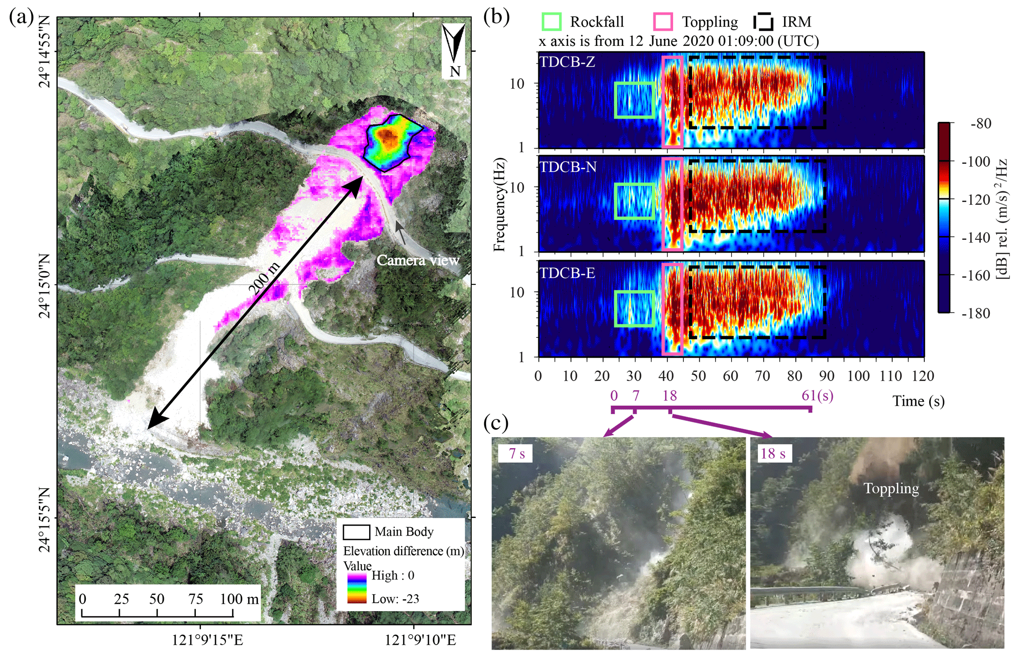
Figure 7 The field photo, spectrograms, and time-lapse photos from a video of a recent RSF on the 12 June 2020. (a) Field photo of the event. The gradient color is the elevation difference between the DTM originating from lidar in 2012 and the digital surface model (DSM) derived from a drone survey after the event. The main body is considered as the elevation difference larger than 3 m. (b) The spectrograms of three components. The top-left corner of the spectrograms shows the station name with the components. The purple axis below the spectrograms indicates the time points from the video. (c) Time-lapse photos from the video corresponding to the physical process of rockfall (left panel) and toppling (right panel). The seconds shown in the top-left corner indicate a time tag in the video.

4.4 GeoLoc scheme applied for rapid report

To test how the GeoLoc scheme, which is composed of source classification, volume estimation, and extraction of physical process, can provide a rapid report, an event that occurred at 01:09 UTC on 12 June 2020 was used. This event was only recorded by the BATS seismic station of TDCB (the epicentral distance of ∼ 600 m). Thus, the location process of the GeoLoc scheme cannot be examined. However, the seismic signals of a closer station would help evaluate the feasibility of carrying out source classification and volume estimation and understanding the event's physical process. With a priori knowledge of source location, we directly compute the seismic magnitude. The result shows the M_L and M_D of 0.36 and 2.75, respectively. A M_L/M_D of 0.13 can yield successful source identification using the threshold of 0.85 proposed in this study. Furthermore, we utilize the peak amplitude of 1.09 × 10⁻³ cm s⁻¹ recorded by TDCB station as the A₀ value for the volume estimation. Application of two regression scaling relations derived in this study (Fig. 5c, d) yield the source volumes (V) of 3838 and 3019 m³, respectively, which are roughly consistent with the preliminary volume of 5142 m³ estimated from the digital surface model (Fig. 7a).

Three-component spectrograms from the TDCB station are shown in Fig. 7b. Based on our simple typology of the physical process, the spectrogram of TDCB was used, and its physical process can be divided into three parts: (i) the pulse-like features that can be observed during the period from 01:09:25 to 01:09:38 UTC (green rectangle in Fig. 7b), corresponding to multiple rockfalls; (ii) the emergent column-shape spectrogram (01:09:38 to 01:09:45 UTC in Fig. 7b) relates to the rock toppling process with mass impacting and/or impact of the boulder rock mass; and (iii) the process finally turned to the complex interactions between the fragmented rock mass and propagation surface with the PSD dominating over 2 Hz of the IRM phase.

To examine the aforementioned physical processes, we obtain the video released by the DGH. At the beginning of the video (the first 15 s), the motion type of the rock mass includes rolling, bouncing, and impacting the hillslope and road surface. The massive rock mass then topples (18 s; Fig. 7c) and hits the slope (19 s), and finally raises a cloud of dust (after 19 s). After aligning the time point (19 s in the video to 01:09:42 UTC) of the peak PSD value with the significant impact inferred from the video, the above spectrogram features are consistent with the motion behaviors extracted from the video, except for the IRM phase. Based on the photos captured by the drones (Fig. 7a), the runout distance is around 200 m, which implies that the mass material continued to move rather than just stop, so it generated a continuous signal of 50 s.

Notably, the real-time broadband waveforms from five stations (CLAB, XAMB, WLUB, ELDB, and SYNB, shown in Fig. 1c) distributed along the southern provincial highway and one station (YULB) outside the Sinwulyu catchment are ready for real-time implementation. Based on the flowchart of the GeoLoc scheme shown in Fig. 2, we first fixed a band-pass filter of 1–8 Hz, which can be applied to most events in this catchment, except for one single boulder impact (Event S5). Certain thresholds of $M_{\mathrm{L}}/M_{\mathrm{D}}$ (0.85) and propagation distance (10 km; see Fig. S8) are used to ensure successful source discrimination. Two scaling lines established in this study are available for rapid volume estimation. However, manual checks are still needed to obtain the signal duration (required for calculating M_D) and physical process, which can easily be automatized by machine-learning-based classification approaches. Since June 2020, the GeoLoc-based monitoring system has been in operation online and is under testing.

5 Conclusions

The GeoLoc scheme has been developed to successfully study 10 RSFs using the seismic signals from permanent and temporary seismic networks, and it provides estimations of the location and associated seismic parameters of the events, namely A₀, α, M_L, and M_D. For the source discrimination, a certain M_L/M_D threshold of 0.85 can essentially classify the sources of RSFs and earthquakes in Taiwan. We further built two regression equations for the V−A₀ and V−M_L relations, which are crucial for estimating the lower bound of source volume after an event occurrence. By analyzing the videos and seismic signals from the nearest station with an epicenter distance of less than 2.5 km, we can comprehensively understand the main physical processes that control the seismic signals' features. For example, the characteristics in spectrograms induced by the multiple rockfalls, the impact of boulder mass (similar to toppling), and the complex interactions between the rock mass and propagation surface that exhibit pulse-like, column-shaped, and V-shaped features, respectively. The aforementioned threshold and limitation are applicable to monitor RSFs in Taiwan; however, for other areas with different geological backgrounds, these values should be varied.

In practice, for events with location quality levels A and B, we can provide information on the source location, volume estimate, and physical process within a short time. For events with quality level C, only the physical process from the spectrogram features can be retrieved. The result of this research is vital for the government to carry out effective emergency responses after an RSF occurrence. Rapid estimation of location and volume would be helpful for effective road control and hazard management. The physical process also delivers a useful message to engineering geologists in order to promote a better understanding the failure mechanisms of RSFs and to aid in designing slope protection plans. Before implementing the GeoLoc scheme in real time, a detailed geological survey is necessary in order to better understand potential failure mechanisms and highlight high-risk slopes. Currently, the GeoLoc scheme shown in Fig. 2 has already been adopted in the Sinwulyu catchment, which is a high-risk area with respect to RSFs in Taiwan, and it could be readily applied in other places with high RSF activity around the world.