Grain size of fluvial gravel bars from close-range UAV imagery – uncertainty in segmentation-based data

Data on grain sizes of pebbles in gravel-bed rivers are of key importance for the understanding of river systems. To gather these data efficiently, low-cost UAV (uncrewed aerial vehicle) platforms have been used to collect images along rivers. Several methods to extract pebble size data from such UAV imagery have been proposed. Yet, despite the availability of information on the precision and accuracy of UAV surveys as well as knowledge of errors from image-based grain size measurements, open questions on how uncertainties influence the resulting grain size distributions still persist.

Here we present the results of three close-range UAV surveys conducted along Swiss gravel-bed rivers with a consumer-grade UAV. We measure grain sizes on these images by segmenting grains, and we assess the dependency of the results and their uncertainties on the photogrammetric models. We employ a combined bootstrapping and Monte Carlo (MC) modeling approach to model percentile uncertainties while including uncertainty quantities from the photogrammetric model.

Our results show that uncertainty in the grain size dataset is controlled by counting statistics, the selected processed image format, and the way the images are segmented. Therefore, our results highlight that grain size data are more precise and accurate, and largely independent of the quality of the photogrammetric model, if the data are extracted from single, undistorted nadir images in opposition to orthophoto mosaics. In addition, they reveal that environmental conditions (e.g., exposure to light), which control the quality of the photogrammetric model, also influence the detection of grains during image segmentation, which can lead to a higher uncertainty in the grain size dataset. Generally, these results indicate that even relatively imprecise and inaccurate UAV imagery can yield acceptable grain size data, under the conditions that the photogrammetric alignment was successful and that suitable image formats were selected (preferentially single, undistorted nadir images).

1 Introduction

Knowledge of the particle size distribution and the shape of channel bars in gravel-bed rivers offers a key to both a scientific understanding of fluvial systems and the ecological management of rivers. In addition, constraints on sediment caliber are critical to understanding the hydraulic conditions, the mechanisms of sediment transport, and the grain–grain interaction during material entrainment, transport and deposition (e.g., Piégay et al., 2020; Tofelde et al., 2021). Information on grain size allows us to quantify the thresholds for material transport (e.g., Shields, 1936; Church et al., 1998), to understand and model the transport of sediment in rivers (e.g., Attal et al., 2015; Dunne and Jerolmack, 2018; Lamb and Venditti, 2016; Whittaker et al., 2010), and to characterize habitats (e.g., Kondolf and Wolman, 1993). It further allows prediction of the probability of sediment entrainment (Schlunegger et al., 2020) and assessment of the impact of infrastructure on material transport (e.g., Grant, 2012). Standard methods that have been developed to quantify grain sizes of gravels in rivers involve time-intensive fieldwork (e.g., the point counting method of Wolman, 1954), which bears the risk of introducing biases that are rooted in the way the measurements in the field are conducted (e.g., Wolcott and Church, 1991; Bunte and Abt, 2001). To reduce the effort and time involved in collecting data by hand, and the possible biases therein, methods for grain size estimation based on image data have received more attention since the early 2000s (e.g., Carbonneau et al., 2004; Butler et al., 2001). These tools have developed into established methods for the quantification of grain sizes in recent years (Carbonneau et al., 2018; Purinton and Bookhagen, 2019; Detert and Weitbrecht, 2012). This development was assisted by the technological improvement in uncrewed aerial vehicles (UAVs) and low-cost photogrammetric software packages, which allow a large number of relatively high-resolution topographic data from images to be collected (e.g., Eltner et al., 2016; Woodget et al., 2018). In particular, the use of the structure from motion technique (SfM; Eltner and Sofia, 2020; Fonstad et al., 2013; James and Robson, 2012) has yielded various topographic datasets, such as digital elevation models (DEMs), ortho-images and ortho-image mosaics, and 3D point clouds. Such data have offered the basis for extracting grain size information from fluvial gravel bars (Woodget et al., 2018). Several studies resulted in the development of methods for the grain size estimation that are tailored to specific UAV workflows and survey designs (e.g., Carbonneau et al., 2018; Vázquez-Tarrío et al., 2017; Woodget and Austrums, 2017). Consequently, over the last few years, significant effort has been directed toward quantifying and reducing the uncertainties related to SfM models (e.g., James and Robson, 2014; Smith and Vericat, 2015; James et al., 2017a, b; O'Connor et al., 2017; Sanz-Ablanedo et al., 2020). In contrast, fewer studies have investigated the impact of these uncertainties on grain size results (Pearson et al., 2017; Woodget et al., 2018). Despite the fact that all data on grain size can only be as precise and accurate as the underlying image or topographic model, a systematic evaluation of the method of choice, which particularly considers the related uncertainties, is still scarce for such data (Piégay et al., 2020). Furthermore, recent work demonstrates that widely used survey strategies and camera systems in UAV platforms might still introduce systematic biases to SfM data (James et al., 2020; Sanz-Ablanedo et al., 2020), thereby pointing to the need to re-evaluate some previous UAV survey recommendations (i.e., survey geometry, image acquisition format and some parameters for camera lens modeling).

This paper addresses this challenge. Here we present the results of three close-range UAV surveys conducted along Swiss gravel-bed rivers (Fig. 1), for which we developed SfM topographic models. From these models, we extracted undistorted nadir images and ortho-images for grain size analysis and for estimates of model uncertainties. Our focus is to assess the dependency of the grain size results on the UAV survey strategy. Consequently, we particularly assess the effect of (i) different image acquisition formats, (ii) specific survey designs recommended by previous authors, and (iii) geo-referencing methods on grain size data. We do so by first employing existing techniques for assessing the uncertainties in topographic models derived from SfM (James et al., 2017a, b, 2020). We then model these uncertainties introduced from the UAV survey to the grain size measurements, which we conduct with an established method (Purinton and Bookhagen, 2019). In particular, we combine the effect of the different UAV and SfM models and their uncertainties with the statistical uncertainties related to the grain size measurements through a combined bootstrap and Monte Carlo (MC) approach.

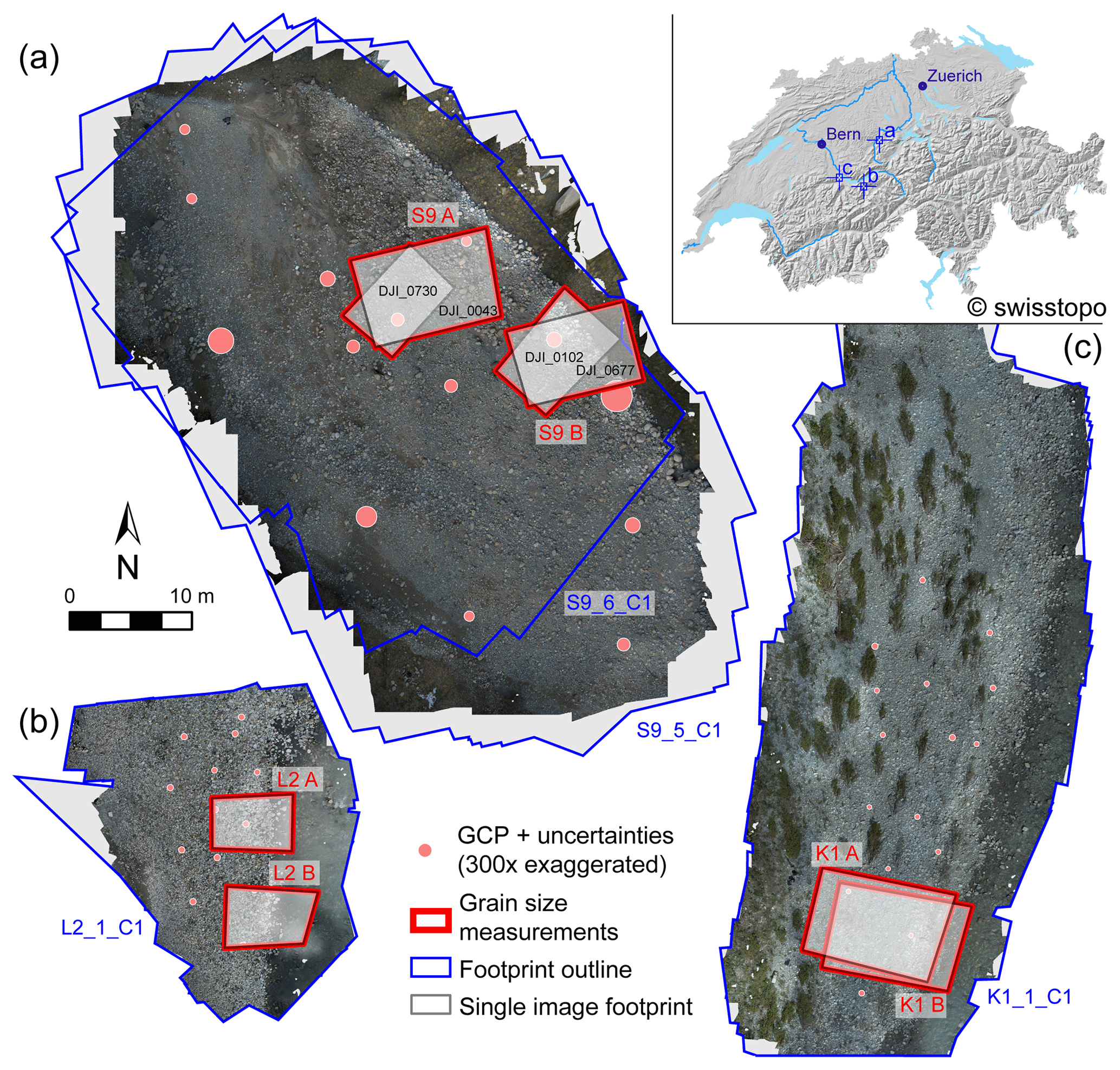
Figure 1 Overview of the surveyed gravel bars along the selected Swiss rivers (see insert) as overview orthophoto mosaic from the most accurate topographic models (see text for discussion): (a) Entle surveys (S9_5, S9_6), (b) Luetschine survey (L2), and (c) Kander survey (K1). Regions A and B, which are used for grain size measurements (both orthophoto mosaic and single, undistorted nadir image) are indicated. GCP: ground control point.

1.1 Approaches to collecting grain size data from digital images

Historically, the collection of grain size data from gravel-bed rivers has relied on time-consuming and laborious physical measurements of clasts in the field (Wolman, 1954; Wohl et al., 1996; Bekaddour et al., 2013; Van den Berg and Schlunegger, 2012; Pitlick et al., 2021). Early image-based grain size measurements were conducted with a “photo-sieving” approach (e.g., Ibekken and Schleyer, 1986), which relied on the visual identification of clasts in images from ground-based cameras. The next step in the improvement of the method was accomplished using two different strategies. The first strategy encompassed methods where grain sizes are inferred from statistical properties of image parameters (e.g., image texture, image spectral or frequency content, point cloud roughness; Woodget et al., 2018). The second strategy, on the other hand, uses approaches where the sizes of individual grains are measured through image segmentation, which refers in this case to the partitioning of an image into multiple image segments, each representing a single grain and thereby belonging to the group of instance segmentation (e.g., Detert and Weitbrecht, 2012; Purinton and Bookhagen, 2019; and references therein).

Most grain size datasets that were collected with the first set of methods were mainly based on a variety of statistical image parameters, such as semivariance (e.g., Carbonneau et al., 2005), inertia, entropy, gray-level co-occurrence matrices (e.g., Carbonneau et al., 2004; Woodget et al., 2018; Woodget and Austrums, 2017), and autocorrelation (e.g., Rubin, 2004; Buscombe, 2008; Buscombe et al., 2010). In this context, other approaches have exploited the roughness pattern of topographic models from 3D point cloud datasets to estimate grain sizes (e.g., Brasington et al., 2012; Woodget and Austrums, 2017). All of these methods require an on-site metric calibration in the field (e.g., with a differential GPS or a meter stick) and only deliver a single percentile of a grain size distribution (Purinton and Bookhagen, 2019). Here, an exception is offered by the wavelet decomposition approach of Buscombe (2013), which is able to determine all the grain size distributions from images without a field-based calibration. However, this only works in a reliable way if grains have nearly the same size and shape. In general, however, the grain size percentile values that resulted from surveys have been found to be highly variable, which depends on the sorting, the shape, and the bedding of the target gravels (Pearson et al., 2017). Such variability in grain size data thus violates the condition of nearly equally sized grains, which is required if one aims to apply the Buscombe (2013) method. Recently, Buscombe (2020) and Lang et al. (2021) have shown that the use of deep learning frameworks allows us to avoid the time-consuming calibration in the field, which facilitates the remote measurements of grain sizes from scaled or geo-referenced images. However, these machine-learning models so far do not allow scales to be readily transferred to new data, with the consequence that the effort that is needed to train the model for a new setting is quite large (Lang et al., 2021).

Methods based on the segmentation and delineation of individual grains in images constitute the second set of tools. Common approaches rely on edge detection and watershed segmentation (e.g., Butler et al., 2001; Graham et al., 2005; Detert and Weitbrecht, 2012). Most recently edge detection and k-means clustering (Purinton and Bookhagen, 2019) or watershed segmentation using deep-learning-assisted semantic segmentation have also been used (Chen et al., 2022). Grain size measurement through image segmentation is challenging for images with a high visual complexity, i.e., overlapping grains, irregularly shaped, colored or textured grains, and vegetation or extensive shadows on the images (Purinton and Bookhagen, 2019). However, the delineation of individual grains in images has the advantage that the result is a continuous grain size distribution. This approach additionally allows the analysis of sub-regions and has the potential to obtain grain size data of individual clast populations, and it offers the possibility of measuring clast orientations.

1.2 Uncertainties related to the photogrammetric structure from motion technique

The rise in widely available and cheap UAV platforms, equipped with stabilizing gimbals and easy-to-use operating applications in combination with low-cost and user-friendly photogrammetric software packages, has resulted in the generation of high-resolution topographic data for various research applications (e.g., Carbonneau et al., 2003; Fonstad et al., 2013; Eltner et al., 2016; Eltner and Sofia, 2020). In this context, the uncertainties and resolution of data processed through SfM (structure from motion technique) especially from UAV images can be predicted from photogrammetric principles. They depend critically on technical (i.e., flight geometry, camera angles, usage of ground control points, camera parameters) and environmental parameters, the latter of which are beyond the operator's control (i.e., lighting conditions, local topography, vegetation, weather, GNSS signal strength). The uncertainties in topographic SfM models can be summarized by three components including (i) the external accuracy of the reference framework (i.e., scaling, rotation or offset of the entire model), (ii) the expected variance of model points (i.e., the 3D tie point variance, sometimes called “precision”), and (iii) a systematic uncertainty component arising from the photogrammetric processing itself (i.e., “doming” or “bowling”). We refer the reader to James et al. (2020), James et al. (2017a, b), and Carbonneau and Dietrich (2017) for a detailed discussion of these uncertainty components. The use of ground control points (GCPs) or the application of differential onboard RTK GNSS (real-time kinematic positioning for global navigation satellite systems) techniques for direct geo-referencing effectively increases the accuracy of the reference framework (James et al., 2017a; Sanz-Ablanedo et al., 2020). Image quality and camera calibration parameters control the level of internal precision (sometimes called “shape” precision; James et al., 2017a). The use of GCPs together with an improved survey geometry and a pre-calibrated camera can significantly increase the internal precision (Carbonneau and Dietrich, 2017; James et al., 2017a, b; O'Connor et al., 2017; Griffiths and Burningham, 2019). In contrast, the occurrence of a systematic uncertainty can only be detected with GCPs and is still a common problem within SfM processing (e.g., Eltner and Sofia, 2020). The successful mitigation of such systematic biases requires a careful choice of the image network geometry, such as the inclusion of oblique camera angles (James and Robson, 2014) and a successful camera lens modeling during the subsequent generation of a model (e.g., James et al., 2020). Finally, it is noteworthy that most uncertainties in models and data from any SfM workflow are derived from the photogrammetric alignment of the images during the generation of the sparse point cloud. Therefore, the uncertainty in the sparse cloud data already includes these uncertainties in the SfM model, independent of the type of the final data model. However, some errors, such as interpolation errors, missing texture, or incorrect matches, might occur during densification or raster generation, thereby affecting some formats only, e.g., orthophoto mosaics.

Despite the possible drawbacks and limitations as outlined above, UAV images have been processed with SfM workflows over the last decade for various research purposes in the fields of fluvial geomorphology and sedimentology (for an overview, see Carrivick and Smith, 2019), including grain size measurements in fluvial systems (e.g., Woodget et al., 2018). Specifically, for automated grain size measurements, Carbonneau et al. (2018) developed the “robotic photosieving” concept, which is based on the use of close-range, single UAV images that have been processed with a specific SfM pipeline (direct geo-referencing, the use of pre-calibrated camera lens models, and surveys with a second flight altitude to better estimate the camera positions). Accordingly, in such an approach, only the image distance is effectively used for scaling. Other methods use orthophotos and orthophoto mosaics (Woodget et al., 2018) or 3D point cloud roughness (Woodget and Austrums, 2017) to measure the sizes of gravels. The applications of these methods have shown that single images are most accurate for grain size estimations, while image textures or 3D point clouds yield measurement results that are less accurate (Woodget et al., 2018). Unfortunately, no systematic evaluation of uncertainties introduced by the UAV SfM approach to such grain size estimations exists so far.

2 Methods

We acquired UAV images (Sect. 2.1) from rivers situated in the Swiss Alps with a widely used platform following established survey strategies, which we processed with an SfM software package (Sect. 2.2). We then used this output to measure the sizes of grains and the uncertainty associated with this (Sect. 2.3). The steps of this workflow (Sect. 2.4) are described below.

Table 1 Summary of the field surveys. QA: quality assessment. Here we removed images that were (i) blurred, (ii) hard to align because of an insufficient depth of field due to camera angles that were too oblique, or (iii) under- or overexposed. GCP: ground control point.

2.1 UAV surveys

We chose study sites along the Luetschine (referred to as L2 surveys), Entle (S9 surveys), and Kander (K1 surveys) rivers that are all situated in the Swiss Alps (Fig. 1). We selected river reaches where gravel bars can be readily identified on satellite images and where the local topography offers the opportunity to operate the UAV in different conditions and with different challenges, i.e., due to vegetation cover, narrow gorges, and steep lateral valley borders. We conducted close-range surveys with a flight altitude between 5 and 7 m above ground to ensure a ground-sampling distance of ∼1.5 mm (Table 1). The close-range setup was employed to study grain size trends on an intra- and inter-bar scale in small mountainous streams. In general, we targeted a lateral and frontal overlap between individual images in the order of 80 %. We distributed GCPs over the target gravel bars and measured them with a Leica Viva GS14 or a Leica Zeno GG04 plus GNSS antenna, with real-time online Swipos-GIS/GEO RTK correction. These setups have a horizontal precision of 2 cm and a vertical precision of 4 cm (for 2σ) under ideal conditions (Swisstopo, 2022). All GCPs and their uncertainties used in this survey can be found in Table S1 in the Supplement.

We diversified the strategy for image acquisition to produce a large range of models, which is considered to resemble a variety of practical scenarios and strategies (Fig. 2). These scenarios are based on recommendations to include oblique angle camera positions (e.g., James and Robson, 2014), images from a second altitude level (e.g., Carbonneau and Dietrich, 2017), and referencing strategies with and without GCPs (e.g., James et al., 2017a, b). All these scenarios and models are summarized in Fig. 2 for the three study areas. Some scenarios are expected to produce topographic models with low accuracy and large systematic uncertainty (e.g., single-level grid with no GCPs as control points). All images were taken with a DJI Phantom 4 Pro v2 onboard camera (DJI FC6310), which utilizes a global shutter. For most flights, images were simultaneously taken in a JPEG and raw (i.e., the unprocessed DNG) image format using the VC Technology's flylitchi application (v2.10.0), except for the S9 surveys. There we used two UAV flight plans, for which we acquired the images first as JPEG files and then, during a second flight, in the DNG format. At the L2 and K1 sites, we first acquired a single grid line map. Subsequently, images were taken with oblique and convergent cameras with a pitch of >20^∘ at the same survey altitude. At site S9, both surveys were done with oblique and convergent camera angles (>20^∘) at a higher flight altitude (∼10 m). This higher altitude included an additional set of nadir images. The images that were taken at a higher altitude and with an oblique view were acquired during manual flying at all sites. A summary of the survey characteristics is provided in Table 1.

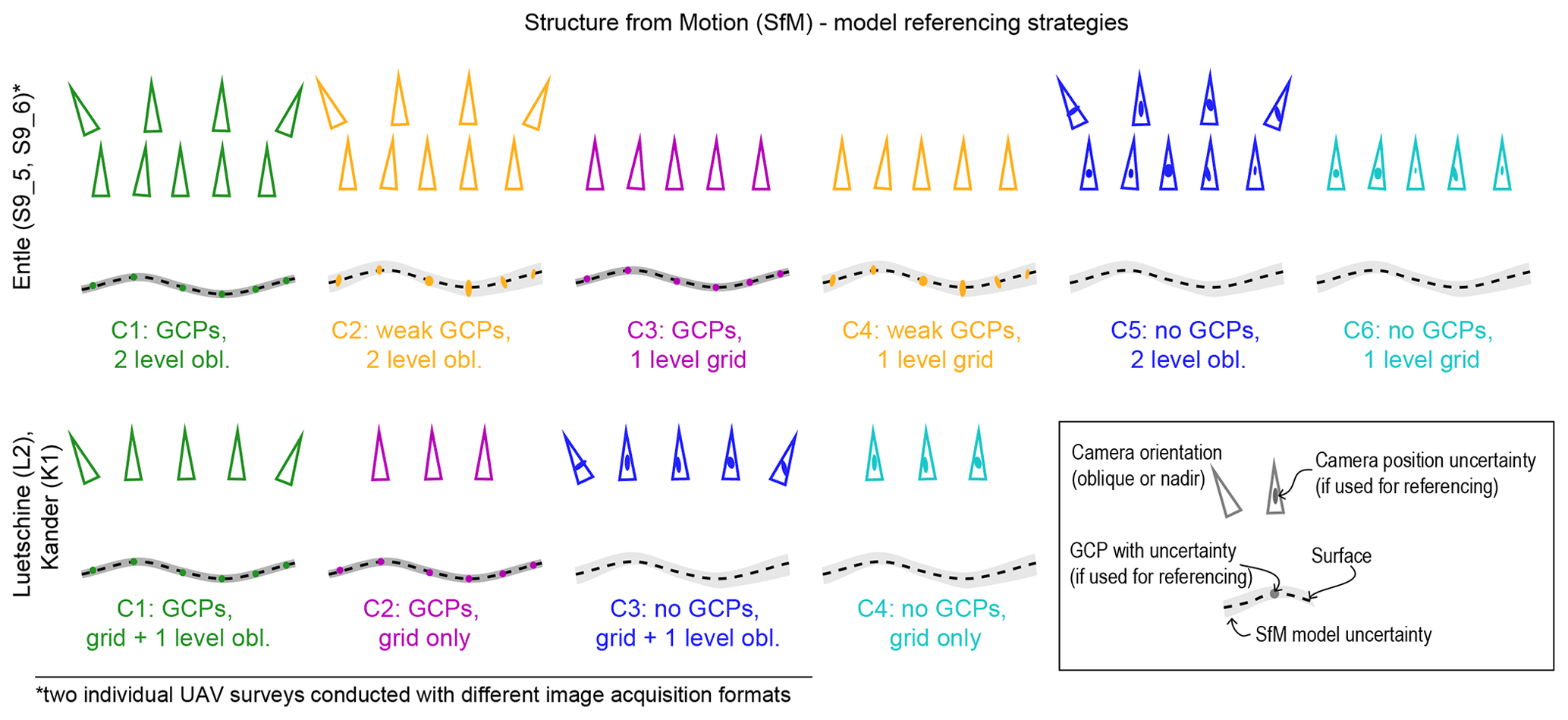
Figure 2 Strategies for UAV surveys and structure from motion (SfM) model setups (upper row: Entle surveys; lower row: Luetschine and Kander surveys). We used a one-level grid of nadir camera positions as backbone geometry, which we complemented with oblique angle camera positions (James and Robson, 2014). At the Entle (S9), we took nadir images at a second altitude (e.g., Carbonneau et al., 2018). We created different models during processing by first including all images and GCPs (i.e., resulting in models with “C1” labels) and then leaving out the oblique images or the GCPs. For the Entle (S9) models we also tested the option where we used the GCP targets in the images as reference markers only, resulting in two additional models that are labeled with “C2” and “C5”. Colors indicate similar model strategies. For flight altitude and nominal camera angles, see Table 1. GCPs: ground control points.

The K1 site at the Kander River offers a setting that is ideal for close-range UAV image acquisition, with little peripheral vegetation and little potential GNSS signal obstruction. In contrast, the L2 site at Luetschine represents challenging UAV survey conditions, due to vegetation and infrastructure limiting the flight area and because of the narrow valley potentially inhibiting the receipt of GNSS signals. The two surveys at Entle (S9) specifically allow us to test the inter-survey comparability and whether a rapid change in the external parameters such as lighting conditions or moving vegetation introduce a bias and whether such a bias would contribute to the uncertainties in the grain size estimation.

2.2 Photogrammetric processing

We generated all topographic SfM models following the same workflow (Fig. 3). We used the Agisoft Metashape (v1.6 Pro; formerly PhotoScan) software, licensed to the Institute of Geological Sciences, University of Bern. We followed the standard bundle adjustment procedure within this software package and refer readers to Eltner and Sofia (2020) and James et al. (2019) for principal descriptions and guidelines of such workflows or to Over et al. (2021) for a detailed example. Our model generation (Fig. 3a) always included (i) the manual removal of blurred images, (ii) the selection of the “highest-quality” settings within Metashape for the initial alignment, and (iii) the subsequent filtering of tie point clouds. In general, we used self-referencing and GCPs for the alignment and standard camera modeling, which included all standard parameters except the de-centering parameter p₂ in order to avoid introducing an additional systematic bias for some models (see James et al., 2020). Only when the camera modeling failed did we employ a pre-calibrated camera model. For these pre-calibrated camera models, we used the in-built camera calibration routine in Metashape, for which we took images of the “chessboard” pattern from different angles with camera distances of 1 to 2 m. For models calibrated with GCPs (ground control points), we included 50 % of the GCPs for the alignment of the images, and we kept the remaining GCPs as checkpoints. For the “weak GCPs” scenario, we used the GCP targets in an attempt to improve the image alignment without using the information on the position that was independently measured.

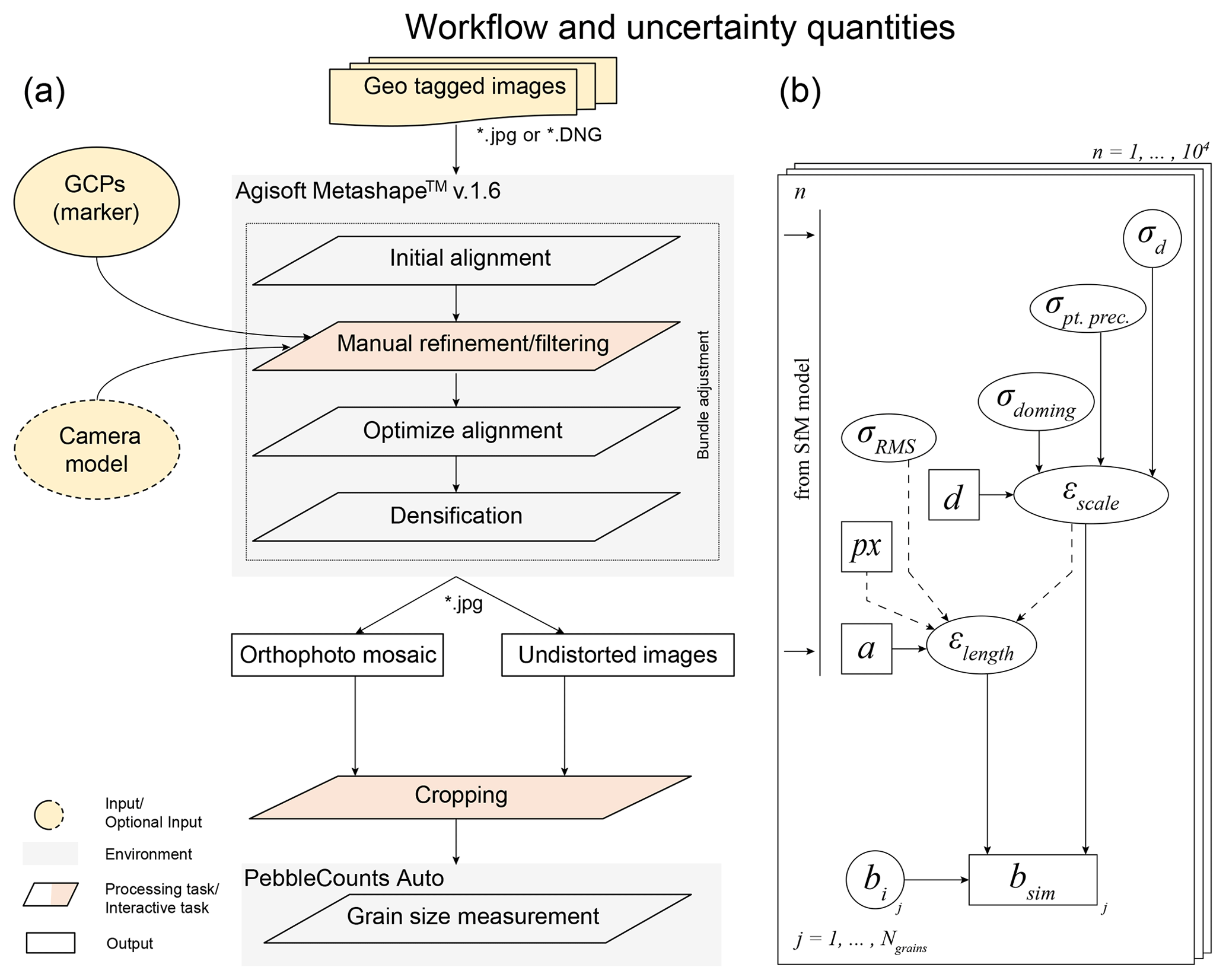
Figure 3 Workflow for grain size estimations from UAV-derived images. (a) Structure from motion workflow with PebbleCountsAuto (Purinton and Bookhagen, 2019) for grain size estimation. (b) Quantities used for estimating the uncertainty in the grain sizes. Quantities in squares denote image- and/or survey-specific values, while variables in ellipses are represented by a probability density function (pdf). Dashed arrows indicate quantities only used for uncertainty estimation in orthomosaics. For variable explanation, see Sect. 2.4 in the main text.

We evaluated the accuracy of the SfM model with GCP residual uncertainty, expressed as root mean square error (RMSE) between measured and estimated checkpoints. To assess the model precision, we used the method (and the Python script) of James et al. (2020) to export and evaluate the sparse point cloud precision from Metashape, which uses Metashape's sparse point coordinate variance as estimates for the precision of oriented and scaled point coordinates. Furthermore, we determined the systematic uncertainty (doming) with the method of James et al. (2020). Their approach is to model the systematic error in the z direction from GCP errors, expressed as a function with a squared radial term, tilting along the horizontal distance, relative to the centroid of the tie points. We report the amplitudes of the modeled doming in the z direction, which are calculated over horizontal distances of 20 m (K1), 12 m (L2), 30 m (S9_5), and 20 m (S9_6), in Sect. 3.

The subsequent orthophoto mosaic generation was accomplished using the “hole filling” option and default blending (“Mosaic”) in Metashape. Orthophoto mosaics were generated with a pixel resolution of 1 mm and were cut with the corresponding camera footprint. We also exported single nadir images, which were undistorted by using the specific camera model from the photogrammetric alignment. We will refer to these single, undistorted nadir images throughout the text as single images. We further estimated the camera height for these images as distance of the camera center to the horizontally closest 100 tie points using Euclidian distances. All imageries (both orthophoto mosaics and single images) were exported from Metashape as a JPEG file, with initial DNG images that were converted by using the camera white balance. We note here that we did not employ any further image processing, such as changing the contrast value for DNG images, to avoid introducing any bias from such approaches. For each study site, we selected specific areas in the model regions (i.e., regions A and B hereafter), for which we then finally determined the grain size distributions. For L2 and S9 we selected areas with expected relative higher and lower model quality, with respect to image multiplicity, tie point precision, and image noise due to water. However, for K1 we opted for overlapping regions to test for effects related to the variability between different images and to allow a comparison of results to those from field measurements.

2.3 Grain size measurements

We measured grain sizes automatically on all processed images with the open-source and Python-based PebbleCounts (i.e., PebbleCountsAuto) software of Purinton and Bookhagen (2019). We employed this software package for two reasons, namely that it yields sizes for individual grain instances and that it allows measuring large numbers of grains in an automated way. First, only the measurement of individual grain instances (which means that each grain is identified, delineated, and recorded) allows modeling specific uncertainty quantities (see Sect. 2.4 below, Fig. 3) taken from UAV–SfM surveys to grain size data. This prohibits the use of texture-based approaches sensu latu, e.g., DGS (Buscombe, 2013), SediNet (Buscombe, 2020), and GrainNet (Lang et al., 2021) among others, to measure grain sizes for the purpose of this study. Second, other segmentation-based approaches, e.g., Basegrain (Detert and Weitbrecht, 2012) or manual segmentation (Sulaiman et al., 2014), require manual processing of each image and are therefore not suitable for the large number of processed images as is the case in this study. We acknowledge that there are known shortcomings of PebbleCounts, and we refer to Chardon et al. (2022) for a comparison with other software results and to Purinton and Bookhagen (2021) for mitigation strategies of some shortcomings.

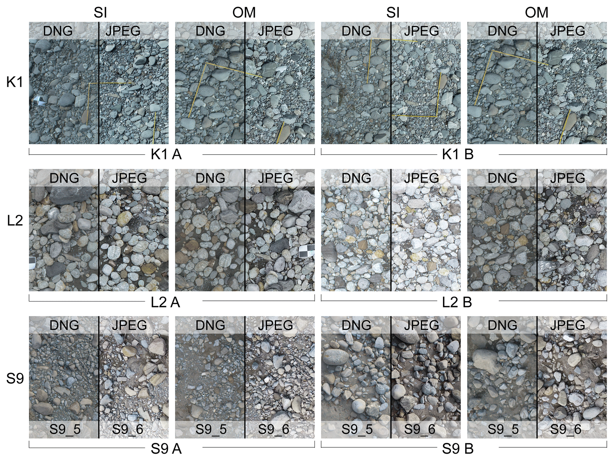
Figure 4 UAV imagery results illustrated by a selected range of images, for both image acquisition formats (JPEG and DNG) that we used for grain size estimation. The photos showcase survey-specific image conditions, e.g., shadows, exposure, saturation, and contrast, as well as site-specific variations, e.g., grain shape, color, or sand content. Please note that all these images, not only orthophoto mosaics (OM), are results that were achieved after photogrammetric processing, i.e., single images (SI) are undistorted with a camera model. All images in this figure were extracted from SfM models, which include GCPs and oblique camera angles in the bundle adjustment. Furthermore, these images only show parts of the corresponding images that were used for grain size estimation. For location reference, see Fig. 1.

In detail, this program segments images and subsequently fits ellipsoids around detected instances of grains, thereby recording the lengths of the a and b axes of these ellipsoids, of which we report the b-axis values throughout the study for simplicity purposes. Key software input parameters were an “otsu_threshold” of 50 and “first_nl_denoise” of 2, and no sand or vegetation mask was used (for further details we refer to Purinton and Bookhagen, 2019). A detection limit of a minimum of 12 pixels for a grain and the default of 30 % as a maximum misfit were kept constant for all measurements. This results in a minimum detection threshold for grains (i.e., a cut-off) that is image specific. For the processed images, this threshold lies around 18 mm given the image pixel resolutions of ca. 1.5 mm px⁻¹. The image resolution, and thus the scale of single images, was estimated individually. To do so, we applied the calculate_camera_resolution script of Purinton and Bookhagen (2019) together with the camera model parameters and the camera distance estimation from the corresponding SfM model. For orthophoto mosaics, the resolution was up-sampled to 1 mm px⁻¹. We cut all grain size data below 18 mm to achieve comparable datasets.

For the Kander survey (K1) we additionally measured the b axis of 250 grains with the approach of Wolman (1954), thereby using a household calliper and a measuring tape. These data were collected as ground truth to compare grain size data measured in the UAV imagery. Yellow rulers in Fig. 4 indicate the area where grain sizes were manually measured.

2.4 Uncertainty estimation

For uncertainty estimation, we used a combined bootstrapping and Monte Carlo modeling approach. We first statistically resampled each grain size distribution (GSD) through random resampling with replacement, i.e., through bootstrapping. We applied 10⁴ iterations to estimate the effect of the sample size. We modeled the one-dimensional uncertainty for each b axis within these resampled GSDs by using uncertainty metrics from the SfM models (Fig. 3b; see also Sect. 2.2), thereby considering that

$$\begin{array}{}\text{(1)}& b_{\mathrm{sim}}=\left(b_i\pm {\mathit{\epsilon }}_{\mathrm{length}}\right)\cdot {\mathit{\epsilon }}_{\mathrm{scale}}.\end{array}$$

Here, b_i is a randomly resampled b-axis value from the measured grain size distribution and ε_length represents the measurement error along the axis length, which can be positive or negative. This error depends on the resolution of the final images that are used for segmentation. We approximate the ε_length term for images with square pixels by taking the pixel diagonal of $\mathrm{2}a\sqrt{\mathrm{2}}$, where a is the average pixel length, multiplied by 2, thereby assuming that at each end of a measured axis represents an error of one pixel. To achieve a randomization in the single image data, we conservatively parametrized ε_length as a normal distribution centered on 0 and with $\mathrm{2}a\sqrt{\mathrm{2}}$ as 1 standard deviation. For the orthophoto mosaics, we employed the same approach to model the measurement errors. However, due to the nature of being a mosaic, an additional error that is sourced in the image alignment might arise since we cannot assume that each pixel is in its correct position in relation to its neighbor. Therefore, we additionally used a shape error in the model (px) expressed in number of pixels, estimated from GCP checkpoints (Table S2), which we convert into length units with the average image resolution estimated from the image distance (see below). Thereby, Eq. (1) changes for values measured in orthophoto mosaics to

$$\begin{array}{}\text{(2)}& b_{\mathrm{sim}}=\left(b_i\pm px\right)\cdot {\mathit{\epsilon }}_{\mathrm{scale}}+{\mathit{\epsilon }}_{\mathrm{length}}.\end{array}$$

Here a represents the orthomosaic resolution, which might be up- or down-sampled. Therefore, our parametrization scales the axis length after adding the uncertainty from the mosaicking, which itself is based on the native image resolution for length scaling. Therein our reconstruction uncertainty (ε_length) is solely governed by the resolution of the final orthophoto mosaic. Furthermore, for the randomization of the shape error, we use a normal distribution centered on the average pixel error in the model as an approximation, while we use the rms re-projection error (σ_rms) as 1 standard deviation of it.

The ε_scale factor, which accounts for the SfM model accuracy, precision, and systematic error (doming), consists of three scaling components. This is parametrized as

$$\begin{array}{}\text{(3)}& {\mathit{\epsilon }}_{\mathrm{scale}}=\mathrm{1}+{\displaystyle \frac{{\mathit{\sigma }}_{\mathrm{d}}+{\mathit{\sigma }}_{\mathrm{pt}.\mathrm{prec}.}+{\mathit{\sigma }}_{\mathrm{doming}}}{d}}.\end{array}$$

Generally, the scale of a nadir image is controlled by the distance between the camera and the ground (d) and the uncertainty associated with this distance. For single images, we estimated the individual camera distance by taking the mean distance in the z direction to the 100 sparse cloud points that are closest to the camera center point. We used a Python script (Supporting information Code S1) for this selection. For randomization, we used this mean as d and its standard deviation as σ_d. For orthophoto mosaics, we used the mean distance of all cameras and the associated standard deviation, respectively. We did so to be conservative and to account for differences between the observation distances of several cameras. We used the mean value of the sparse point cloud precisions in the z direction over the whole survey. We used the 3D point coordinate variance of the sparse point cloud within Metashape, which we exported from the program using the script of James et al. (2020). We used its average in the z direction, and we considered the standard deviation of it to randomize ${\mathit{\sigma }}_{\mathrm{pt}.\mathrm{prec}.}$, both for single images and orthomosaics. Finally, we considered the effects related to the systematic errors through the use of half of the doming amplitude in the z direction, which we fitted with the method of James et al. (2020). We used this value as a standard deviation for a uniform distribution for σ_doming, both for single images and orthomosaics. We implemented a randomization of these components through truncated normal distributions to avoid ending up with grains that are smaller than the detection limit or that have negative length values. We note here that our one-dimensional approach requires a camera model to correct image distortion to a level of residuals being ∼1 pixel or less. We thereby consider the condition that the camera model sufficiently allows for distortion modeling. While it is possible to increase quantities, i.e., the shape error uncertainty for orthophoto mosaics or the ε_length uncertainty to values greater than two pixels for single images, to mitigate the effect of large doming/bowling or high camera model residuals, we currently refrain from such efforts. We do so because we argue that (1) it might be more useful to improve the photogrammetric alignment and (2) such errors show strong variations in space, and therefore our one-dimensional approach might not be suitable anymore. Here, a two-dimensional approach (or even 3D if one attempts to estimate grain size and shape by point cloud segmentation) which would use spatial discretized uncertainties might be more useful. Such an approach, in addition to our considered errors, could also include spatially distributed camera model errors (e.g., Hastedt et al., 2021). For the time being, we did not implement such an approach because of the expected higher computational costs and the expected much higher contribution of counting statistics and segmentation performance to grain size uncertainty.

From the randomized GSD, we calculated percentile values for grain sizes. Accordingly, for each grain size percentile such as the D₅₀ and D₈₄, we report the median percentile along with percentiles 2.5 and 97.5 across the 10⁴ GSDs, which represents the 95 % confidence interval of the respective percentile.

3 Results

In this section, we first present the results of the UAV field surveys, before proceeding to the results of the photogrammetric models. Finally, we present grain size results, both for full grain size distributions and for key percentile values, and results of field measurements.

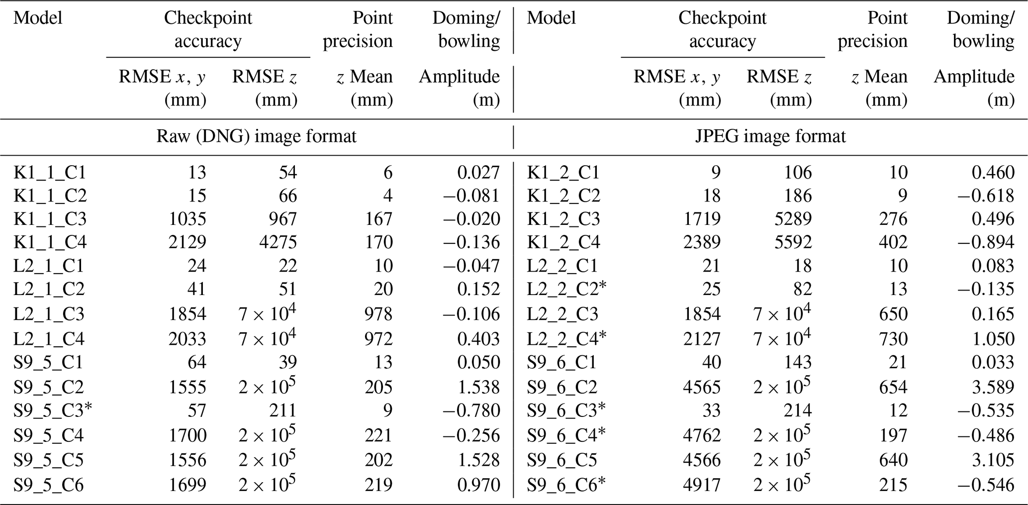
Table 2 Summary of topographic model uncertainty (i.e., SfM model quality). An ^* indicates a model with a pre-calibrated camera model. We note here that the accuracy values for directly referenced models include systematic GNSS errors of up to 200 m (S9) for the UAV platform, an issue that has been reported for the UAV platform family used in our study (e.g., Cook and Dietze, 2019).

3.1 UAV surveys and imagery

The field surveys were successfully completed under sunny and calm (Kander), overcast and turbulent (Luetschine), and rapidly changing weather conditions (Entle). Difficult flying conditions (changing light and wind) decreased the image quality, which contributed to the need to exclude a significant number of images for the Luetschine (up to 27 %) and Entle (up to 20 %) surveys (Table 1). For the Entle site we removed nadir images taken from a higher altitude, and for the Luetschine reach we excluded images that were acquired with strongly oblique view angles (>50^∘). It is noteworthy that most of them were taken during manual flight and, for the Entle case, from the higher altitude level. Acquiring images in the raw format (DNG) required significant reduction in flight velocity due to the low flying altitude. It also required a change in acquisition mode that allowed the UAV to hover for 4 to 5 s at each image position. This was needed to enable saving the large image file to memory. This resulted in net flight times of >30 min for each of our survey sites (Table 1), which exceeded two battery charges for our platform.

The obtained UAV images displayed a range of differences in image content and light conditions (Fig. 4). Sunny situations result in more interstitial shadows (K1, S9), while overcast conditions with changing light led to occasional overexposure (L2). Of note here is site S9, which features more sandy areas then the other sites. Generally, UAV onboard image corrections tend to yield a higher saturation and contrast in the resulting imagery, which was persistent after photogrammetric processing (Fig. 4).

3.2 Topographic models

In total, we produced 28 topographic models with the SfM approach. For all sites, the resulting models show large variations (Table 2) in absolute accuracy, sparse point cloud precision, and systematic error (doming). In general, the uncertainty is smallest across all metrics for model setups for surveys that included GCPs and oblique camera angles (C1 suffix for all surveys). The only exceptions are those models where GCPs and only grid-aligned cameras were used (C2 suffix for K1, L2 surveys and C3 suffix for S9 surveys), thereby resulting in a sometimes slightly higher point precision (Table 2). Overall, models with no GCPs and where cameras were only oriented in a grid fashion (suffix C4 for K1 and L2 surveys and suffix C6 for S9 surveys) produce the highest uncertainties across all metrics. Models that are based on raw format images (K1_1, L2_1 and S9_5 models) yield overall smaller uncertainties for all metrics than models where the UAV onboard pre-processed JPEG images were used (K1_2, L2_2, S9_6 models). Only for L2 JPEG models with GCPs (L2_2_C1, _C2) are the RMSE and vertical precision values slightly smaller than or similar to the related values of comparable DNG models (L2_1_C1, _C2).

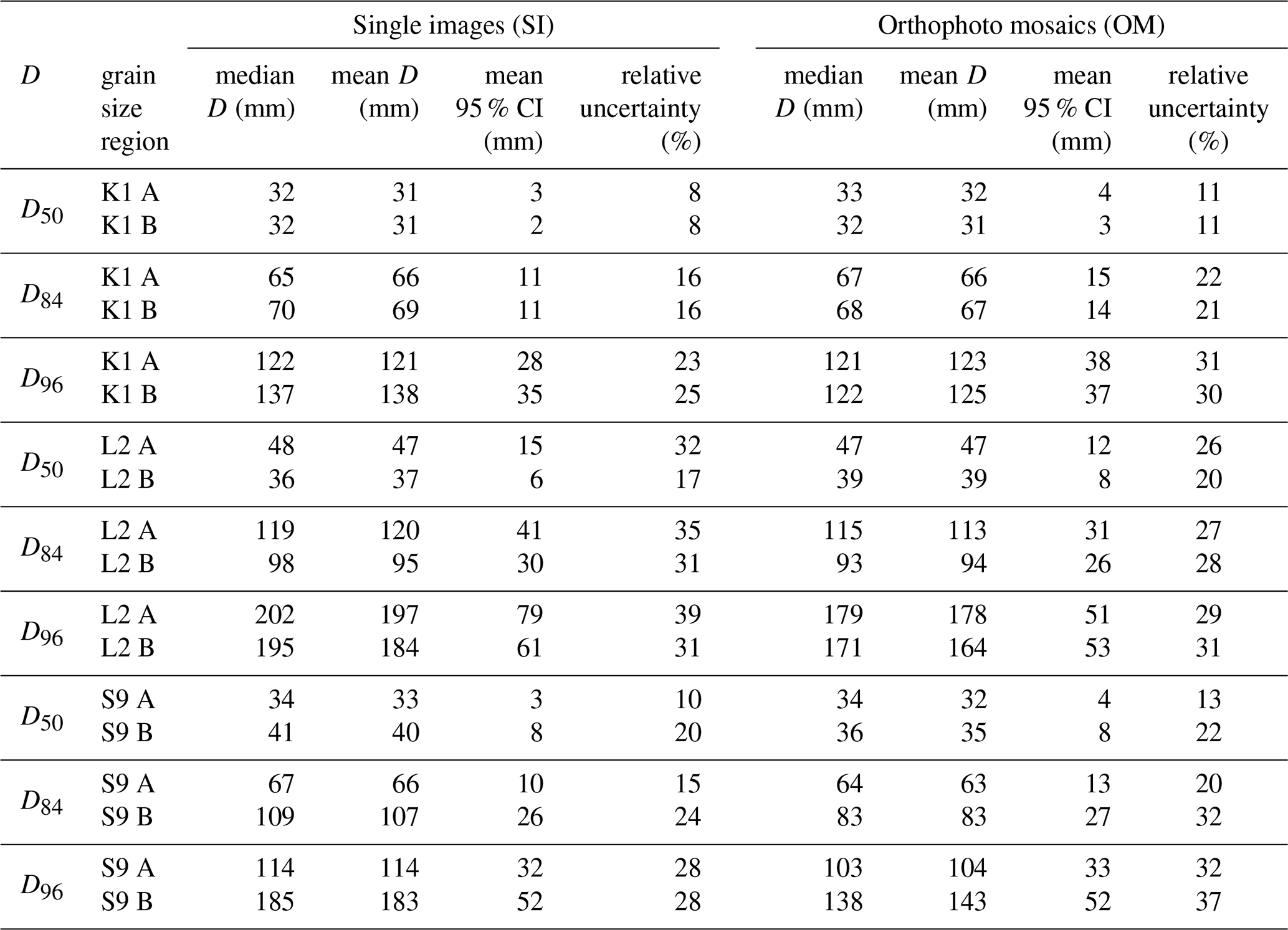
Table 3 Key modeled percentile results (i.e., D₅₀, D₈₄, and D₉₆) averaged over all models for each grain size region.

3.3 Grain size distributions

Here we report the results of our grain size measurements from images as GSDs and the respective modeled uncertainties, which encompass both statistical uncertainties and errors introduced by topographic models. We successfully measured grain sizes of pebbles from all 28 SfM models, resulting in 112 complete GSDs (for each topographic model we measured in two regions, both in single images and orthophoto mosaics, respectively) with b axes that range in size from the cut-off of 18 mm to >35 cm. The number of identified grains ranges for the Kander survey (K1) from 902 to 1600 (single images; SI) and 353 to 1142 (orthophoto mosaics; OM), for the Luetschine survey (L2) from 130 to 633 (SI) and 136 to 570 (OM), and for the Entle surveys (S9) from 333 to 1451 (SI) and 160 to 1058 (OM). In all surveys and in most cases, more grains are recovered after segmentation in single images compared to the number of grains found in orthophoto mosaics (Table S4; see also Figs. 5 and 6). Grain size distributions with uncertainties for each percentile can successfully be modeled with the bootstrapping and MC approach for all models (e.g., Figs. 5 and 6). The difference between the median of all photo-measured and all modeled percentiles ranges from 2.0 % to 3.5 % (SI) and 2.5 % to 5.7 % (OM) for survey K1, from 0.9 % to 3.6 % (SI) and 1.4 % to 4.1 % (OM) for survey L2, and from 0.9 % to 8.9 % (SI) and 2.6 % to 9.2 % (OM) for both S9 surveys. These values are relative to the photo-measured percentile values. We note that even the maximum difference between the photo-measured percentiles and the modeled median for the percentiles is generally <10 % for most percentiles. The only exceptions are some models of K1_2 (SI: 11 % to 17 %), L2_1 (SI: 25 % to 47 %; OM: 10 % to 16 %), and L2_2 (SI: 31 % to 36 %; OM: 11 % to 20 %; see Table S4 for all results). Therefore, recovered grain size distributions from imagery are internally consistent within the modeled 95 % CI (confidence interval) for each percentile and for all topographic models (e.g., Figs. 5 and 6), despite some variations in magnitude of uncertainty and a varying degree of agreement across models within surveys.

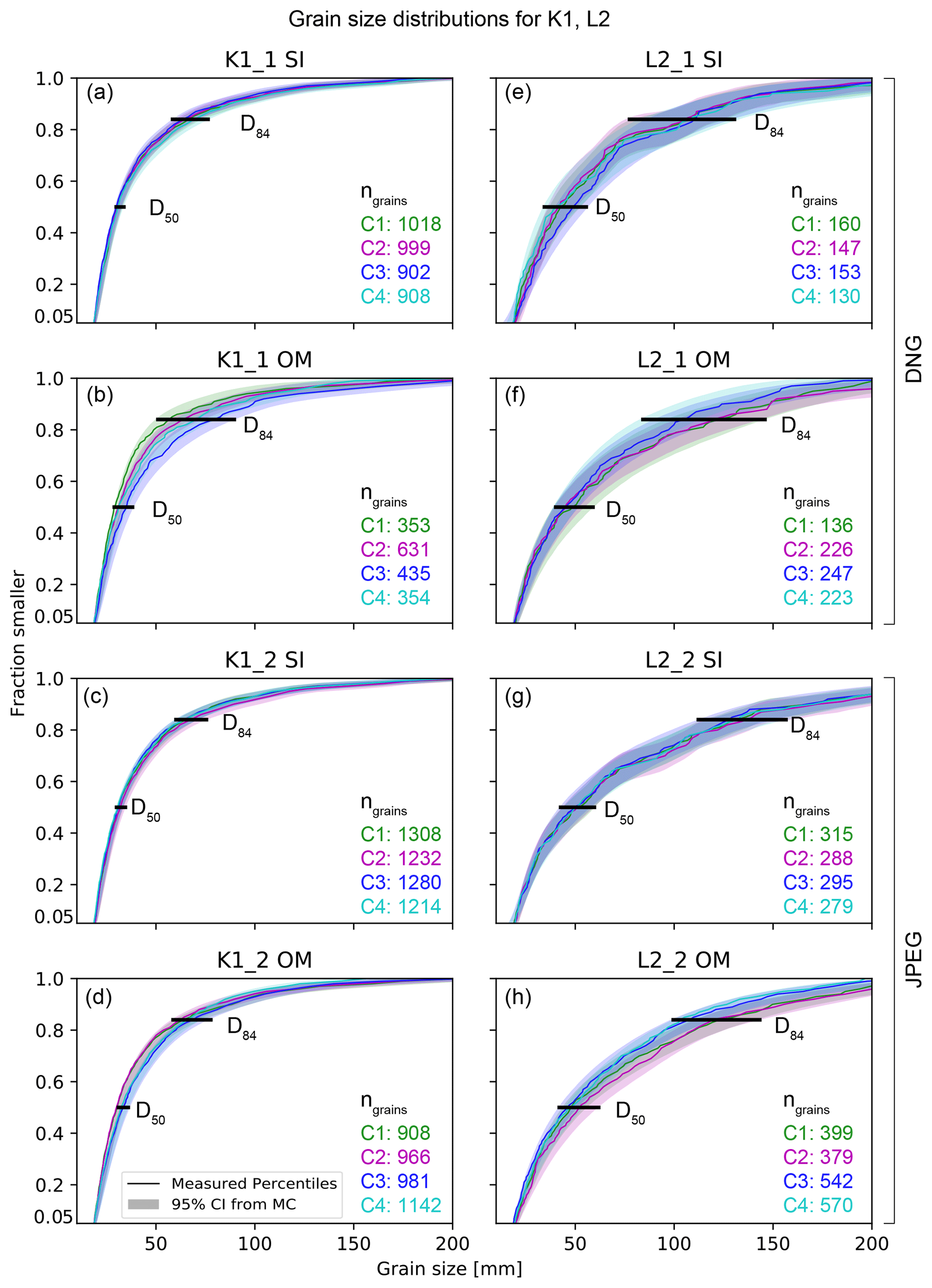
Figure 5 Selected grain size (i.e., b-axis length) distributions measured in different images (SI: single image; OM: orthophoto mosaic) from various UAV models (see Fig. 2 for model characteristics and color legend) with the modeled 95 % confidence interval (CI) for each percentile. All Kander (K1) data (a–d) in this figure refer to region A, while all Luetschine (L2) data (e–h) correspond to the respective region A (see Fig. 1 for location). DNG: raw image acquisition format; JPEG: JPEG image acquisition format; D₅₀, D₈₄: percentiles 50 and 84, respectively; n_grains: number of segmented grains.

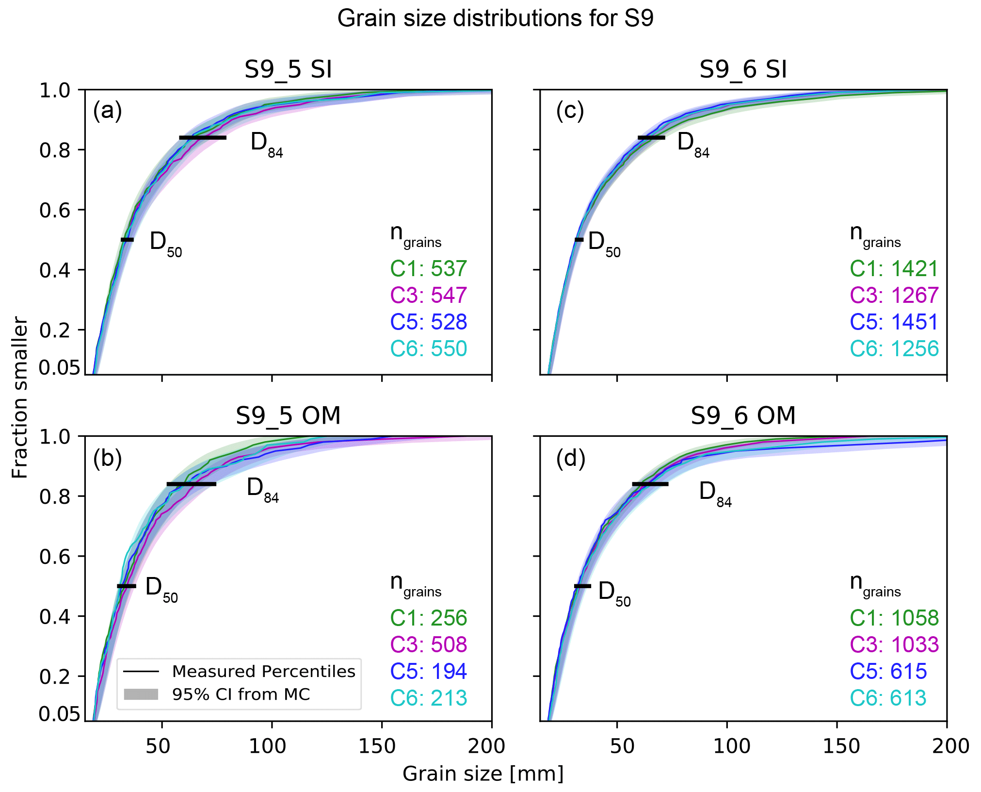
Figure 6 Grain size distributions and percentile uncertainty (modeled 95 % confidence interval; CI) for the Entle surveys (S9) for different UAV imagery (SI: single image; OM: orthophoto mosaic; see Fig. 2 for model characteristics and color legend). All data refer to region A (see Fig. 1 for location). D₅₀, D₈₄: percentiles 50 and 84, respectively; n_grains: number of segmented grains. Please note that S9_5 (a, b) was acquired in raw image format (DNG), while S9_6 images (c, d) were acquired as JPEG images.

The magnitude of grain size uncertainty varies for surveys and the image format used for grain size measurements. Generally, the modeled percentile uncertainty, i.e., the modeled 95 % confidence interval (CI), is smaller for all GSDs from imagery of the K1 survey (e.g., Fig. 5a to d) than for GSDs from the L2 survey (e.g., Fig. 5e to h). A similar trend of survey-specific grain size uncertainty is also visible when comparing results from S9_5 (Fig. 6a and b) to data from S9_6 (Fig. 6c and d). This is also observable in the CI as relative uncertainty, which varies from 6.5 % to 9.4 % (SI) and 7.7 % to 15 % (OM; Fig. 5b and d) for K1. Similarly, albeit with a generally larger magnitude, the modeled percentile uncertainty for L2 ranges from 15.6 % to 41.5 % (SI) and 15.6 % to 37.2 % (OM), whereas it ranges from 7.6 % to 21 % (SI) and 8.2 % to 28.7 % (OM) for the S9 surveys. However and importantly, the agreement of data from models within a survey (i.e., C1 to C6; see Sect. 2.2 for details) is higher for grains measured in single images (e.g., Figs. 5a, c, e, g and 6a, c), compared to grains measured in their orthomosaic counterparts (e.g., Figs. 5b, d, f, h and 6b, d).

3.4 Key grain size percentiles

Overall, modeled percentile medians for commonly used percentile values, i.e., D₅₀, D₈₄, and D₉₆, are in agreement with the photo-measured percentile values for all results and averaged across all models (Table 3; see Table S5 for more details). However, the modeled estimations for the D₅₀, D₈₄, and D₉₆ and their respective uncertainties, here reported for a 95 % CI, vary considerably between individual surveys (Table 3), regions within surveys (Fig. 7), and the format of the images that are used for measuring the grain sizes (Fig. 8).

Figure 7 Modeled median grain size percentile D₅₀ plotted against the D₈₄ for all surveys: Kander (a, b), Luetschine (c, d), Entle (e–h), and regions of grain size sampling (A and B). For locations of the regions, see Fig. 1. OM: orthophoto mosaics: SI: single images.

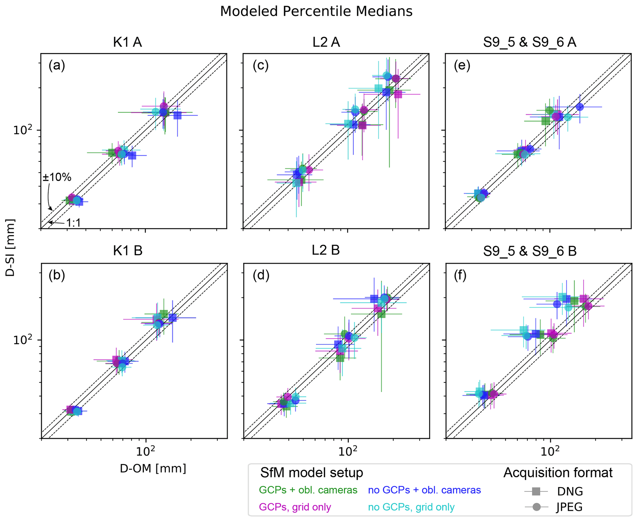
Figure 8 Modeled median values for percentiles D₅₀, D₈₄, and D₉₆ from single images (SI) and orthophoto mosaics (OM) for selected regions of the survey sites. Different SfM model setups are color-coded; please see Fig. 2 for detailed legend. Displayed uncertainties represent modeled 95 % confidence intervals. Please note the logarithmic scale.

For all grain sizes measured in the K1 survey the mean D₅₀ with [3.1–3.2] ± [0.1–0.2] cm, the mean D₈₄ with [6.6–6.9] ± [0.6–0.8] cm, and the mean D₉₆ with [12.1–13.8] ± [1.4–1.9] cm are consistent and in close agreement (Table 3). This is true irrespective of the image region (Fig. 7a and b), the image format used for grain size measurement, or the UAV image acquisition format (Fig. 8a and b). Percentiles from the L2 survey, e.g., the D₅₀ with 4.7 ± [0.6–0.8] cm for region A and with [3.7–3.9] ± [0.3–0.4] cm for region B, are consistent within regions (Table 3). However, the modeled uncertainties are too large to establish differences in percentiles between regions (e.g., Fig. 7c and d), or between model reference strategies, UAV image acquisition formats or between imagery formats (Fig. 8c and d). For percentiles from data for the S9 surveys, the situation is different. Here, key percentile values only agree within regions when extracted from single images (Fig. 7e and g), e.g., yielding a clearly distinguishable D₅₀ of 3.4±0.2 cm for region A and 4.1±0.4 cm for region B. Thus, the averaged percentile values from orthomosaics (Table 3) would yield biased information, effectively prohibiting a distinction of different grain size signals of the regions (Fig. 7f and h). A closer inspection reveals that within the data from orthomosaics only imagery from SfM models, referenced without GCPs (i.e., C5 and C6; see also Fig. 2) and for one single region (B) is responsible for the inconsistent data.

3.5 Field measurements at the Kander site (K1)

The manual measurements of grains sizes > 1.8 cm in the field with the Wolman method yielded 224 b-axis values for K1. The resulting key percentile lengths are 2.8 cm (D₅₀), 5.3 cm (D₈₄), and 10.2 cm (D₉₆). For direct comparison, we measured grain sizes in cropped subsections of all K1 imagery, which returned 162 to 302 (SI) and 189 to 486 (OM) grains. The median of the relative percentile uncertainty (95 % CI) ranged from 14.4 % to 19.5 % (SI) and from 12.7 % to 21.9 % (OM). Mean modeled key percentile values ranged between 3.0±0.3 cm (SI; rel. 16 %–17 %) and 3.2±0.3 cm (OM; rel. 16 %–17 %) for the D₅₀. The mean modeled D₈₄ ranged between [5.9–6.1] ± [1.0–1.1] cm (SI; rel. 33 %–36 %) and [6.5–6.7] ± [1.0–1.1] cm (OM; rel. 30 %–31 %), while the mean modeled D₉₆ ranged between [11.6–12.2] ± [3.0–3.4] cm (SI; rel. 48 %–57 %) and [11.5–12.0] ± [2.4–2.8] cm (OM; rel. 42 %–45 %). These values are in good agreement with modeled results for whole regions (see Sect. 3.4 above and Table 3).

4 Discussion

Measurements of grain sizes in imageries obtained by a UAV need to be accompanied by photogrammetric processing of the imageries to correct for camera lens distortion and to reference the images. Therefore, we begin by discussing the quality of our models and UAV imagery, as well as the conditions encountered in the field. We emphasize here that the aim of this study is not to optimize or review UAV strategies or SfM processing; thus, we restrict ourselves to report only noteworthy observations and their implications in Sect. 4.1. For more in depth discussions of UAV and SfM workflows, we refer to the dedicated literature (e.g., James et al., 2017b, 2020; O'Connor et al., 2017; Carbonneau and Dietrich, 2017; Eltner and Sofia, 2020). Furthermore, we emphasize that our survey design is tailored to close-range studies for the scale of individual gravel bars, which means that while our findings in many ways are transferable to other scales, our survey design might not be applicable for larger-scale surveys (e.g., Marchetti et al., 2022). Next, we focus on the process for measuring grain sizes and for modeling the uncertainties. Finally, we compare the results where grains were measured in images and in the field with the Wolman (1954) method. We then end with a discussion of how grain size data and their uncertainty depend on the various processing steps from UAV image acquisition to estimates of percentile values.

4.1 UAV imagery and SfM model quality

We successfully created topographic models from the image sets collected at the three survey sites. The topographic models are generally better for the Kander (K1) survey compared to the Luetschine (L2) and Entle (S9) surveys (Table 1). We attribute this to the better light and flight conditions (i.e., constantly sunny and weak wind), to lower RTK GNSS (real-time kinematic positioning for global navigation satellite systems) uncertainties, and the more favorable angle and distribution of oblique camera positions (i.e., oblique cameras at the same altitude as the nadir positions and with an angle of 20^∘). In our specific case, vegetation seemed to have a lower impact on the precision of the SfM model quality, since the site K1 was characterized by the highest vegetation density on the bar (Fig. 1), yet the resulting models had the overall highest quality for all metrics. However, our different referencing strategies (Fig. 2) allowed us to create topographic models with varying precision, accuracy, and systematic errors for all surveys (Table 2), in which we find some noteworthy SfM characteristics.

First, some SfM models (see Table 2) failed to successfully reference the images; i.e., they specifically failed to model the camera lens, thereby yielding completely wrong focal length estimations (>50 % rel. difference), which then resulted in camera altitudes that were >50 % lower than the actual flight altitude. Interestingly, significantly more camera models failed for those surveys where the images were acquired in the JPEG format than compared to those models that are based on images in the DNG format (five compared to one). We suspect that this is a consequence of the UAV onboard pre-processing of images with a generic camera model, which results in camera modeling failure during the bundle adjustment (for a detailed discussion, see James et al., 2020).

Second, surveys where images were referenced with GCPs and where images taken with oblique camera positions were included produced the most accurate and most precise models (see Fig. 2 and Table 2). These results fit with our current understanding of SfM uncertainty (e.g., James et al., 2020; Sanz-Ablanedo et al., 2020). Furthermore, we can confirm that the selection of two flight altitudes, as proposed in some workflows for direct georeferencing (e.g., Carbonneau et al., 2018), seems not to improve the quality of the SfM model (see also Sanz-Ablanedo et al., 2020).

Finally, we highlight that for the K1 survey, models that are based on images taken in the JPEG format have a significantly larger systematic error, which is in stark contrast to the models where the images were taken in the DNG image format (Table 2). We note that we cannot use the S9 models for such a comparison, since for these models separated flights were used to acquire the JPEG and DNG images (Table 1). Nevertheless, the aforementioned results suggest that the image acquisition format affects the quality of the SfM model, as already found by James et al. (2020), and even inhibit an alignment for weak image network geometries. Accordingly, the format of image acquisition might be considered during survey planning, as the raw format can indeed yield better results than images in the JPEG format.

4.2 Precision and consistency of grain size measurements

The approach where we automatically segmented the images and where we fitted the ellipsoids with PebbleCounts (Purinton and Bookhagen, 2019) yielded consistent results when measuring grain sizes, both within surveys and between surveys (Figs. 5 and 6; Tables S4 and S5). The combined bootstrapping and Monte Carlo (MC) approach allowed us to estimate the difference between the modeled and the photo-measured median percentile value, which is less than 5 % for single images and 10 % for orthophoto mosaics for all percentiles (Table S5). Thus, both the modeled median and 95 % confidence intervals are representative of the grain size distributions measured in the photos. The median of the modeled percentile uncertainty (95 % CI) relative to the photo-measured percentile varied between survey sites (∼7 % to 15 % for K1, ∼16 % to 42 % for L2, and ∼8 % to 29 % for S9; Table S4). Similarly, the mean relative uncertainties (95 % CI) for individual percentiles, such as the D₅₀, varied from ∼8 % to 11 % for K1, ∼17 % to 32 % for L2, and ∼10 % to 22 % for S9 (Table 3). Relative uncertainty values for the D₈₄ and D₉₆ increased, compared to the D₅₀, but followed the same trends with up to a 39 % relative uncertainty for the D₉₆ in L2. These results allow us to identify two different grain size populations for regions A and B in the S9 surveys (Table 3 and Fig. 7e–h). For K1 where the sampling regions were almost identical (Fig. 1), all grain size results were consistent (Table 3 and Fig. 7a, b; see also Table S5). For L2, the large uncertainties prevent us from drawing such inferences (Fig. 7c and d). At a closer inspection, these findings have some interesting implications.

In particular, because the modeled percentile uncertainty depends on the number of grains that could be identified, i.e., on the counting statistics, the percentile precision improves with a larger number of measured grains (Table S4). This is what we observed, and such results are in good agreement with reported statistical uncertainties that resulted from the application of comparable methods (Eaton et al., 2019). We note here that in general fewer grains were found in images that were acquired in the DNG format. This might be a result of lower image contrast in these images, which we did not attempt to correct. While the smaller number of grains might reduce the percentile precision for images with very few grains in them, we could not find any further systematic effect thereof. In contrast, our data showed systematic differences if grain sizes were measured in single images (SI) or on orthophoto mosaics (OM). Grain size percentiles derived from orthophoto mosaics showed higher uncertainties than grain sizes measured in single images, both for the entire range of percentiles (Figs. 5 and 6) and for selected percentile values (Figs. 7 and 8). L2 is an exception, where the uncertainty in the median grain size percentile was generally high (up to ∼42 %). Compared to the grain size data collected from orthophoto mosaics, the relative percentile uncertainty in the single image data was between 3 % to 6 % lower for K1 and between 0.6 % to 8 % lower for S9 surveys. Likewise, for individual key percentile values, i.e., the D₅₀, D₈₄, and D₉₆, the uncertainties in the data retrieved from orthophoto mosaics were between 2 % and 9 % higher across all models of K1 and S9. However, we acknowledge that for some L2 models, the uncertainties in the grain size data were higher if the data were collected from single images than if the measurements were accomplished on orthophoto mosaics. We attribute this to a combination of imagery and segmentation traits (see Sect. 4.4).

4.3 Grain size accuracy compared to field measurements

Grain sizes in close-range UAV imagery through image segmentation are measured in a 2D approximation of a 3D surface of particles, which might be affected by the sedimentary structure, e.g., imbrication or armoring, and projection effects. Additionally, a bias could be introduced during the segmentation of the images. Therefore, we compare the sizes of grains measured in a subset of the K1 imagery with a dataset where the grains were manually measured in the field to test how our grain size estimations hold up against field-measured data (Fig. 9).

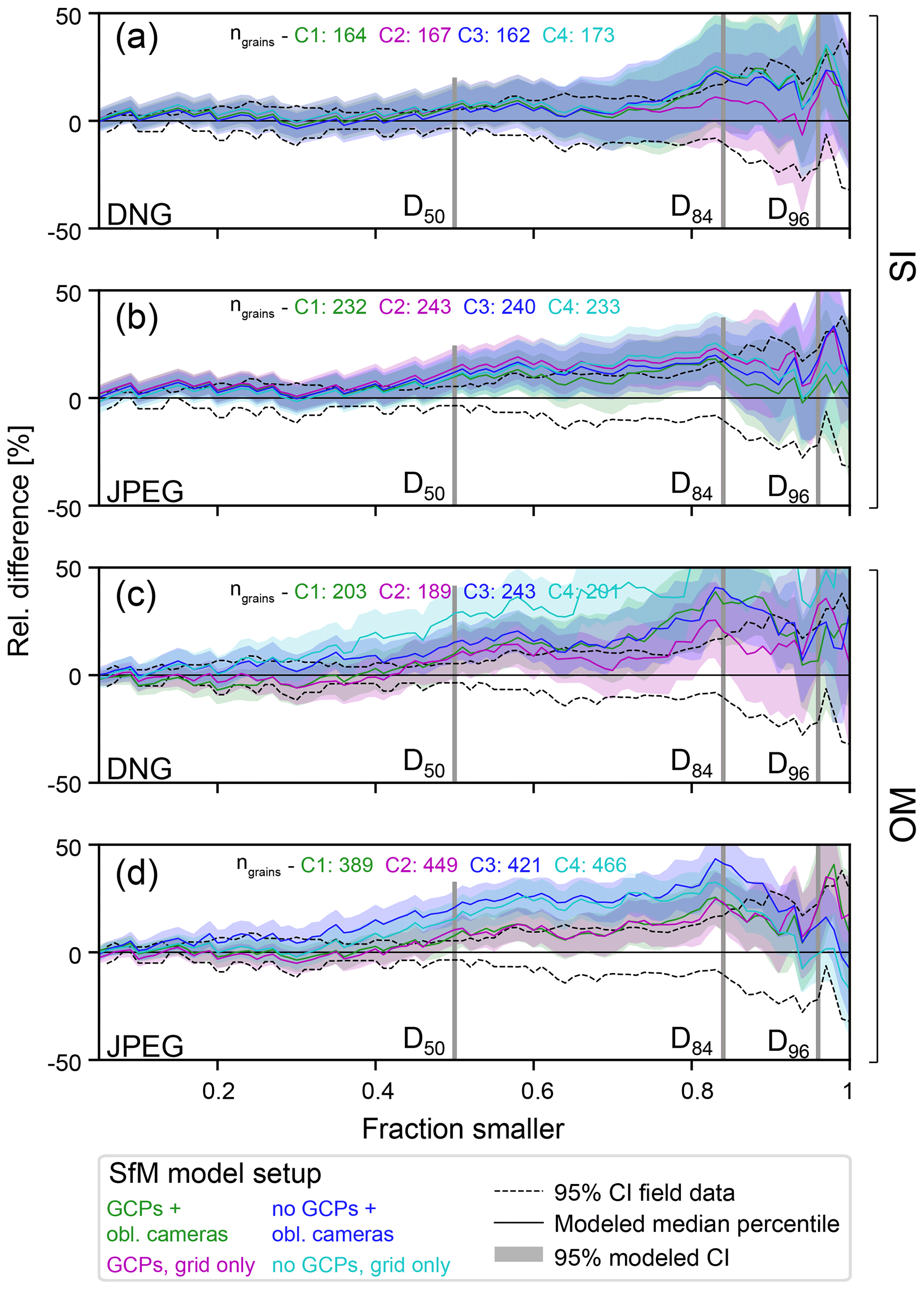
Figure 9 Relative difference between grain size percentiles estimated from UAV imagery to grain sizes, which were measured in the field for region A of the Kander survey (K1). (a, b) Results for data from single images (SI). (c, d) Results for orthophoto mosaics (OM). DNG and JPEG indicate the image acquisition format. Key percentiles, i.e., D₅₀, D₈₄, and D₉₆, are highlighted. The number of detected grains (n_grains) and the data are color-coded for SfM model setup (see Fig. 2 for detailed legend).

First, imagery-based grain size measurements result in an overestimation of the percentile values compared to field-based surveys (Sect. 3.5), independent of the SfM model referencing strategy (Fig. 9). Such a systematic overestimation of grain sizes can even be found for models where the bundle adjustment was accomplished with ground control points and from single images (i.e., C1 and C2 curves in Fig. 9). This is most likely a result of an under-segmentation of grains in images; potential biases inherent in image-based approaches, i.e., a 2D projection effect or partial overlapping of grains (Carbonneau et al., 2005); and/or a combination thereof. We note here that this systematic overestimation might have also have a survey-specific component. We base this inference on the results of other analyses, which were accomplished with the same segmentation software and which documented a systematic underestimation of related percentile values, thus hinting at an effect related to over-segmentation (Chardon et al., 2022). This issue might be addressed if (i) images are segmented semi-automatically where manual measurements are accomplished occasionally to set a benchmark (Purinton and Bookhagen, 2021), (ii) reference measurements are conducted for calibration purposes (Chardon et al., 2022), or if (iii) the automated segmentation is improved. However, more research is needed to improve our understanding of systematic traits of segmentation-based grain sizes and the related dependency on survey-specific characteristics. We note that our K1 site where we did find this bias is not suited for such an endeavor.

Second, for all our K1 models, only grain sizes taken from single images (Fig. 9a and b) can be regarded as acceptable, i.e., agreeing within uncertainties, despite a systematic overestimation of the percentile values. Contrarily, grain size data from orthophoto mosaics are less accurate than from single images when compared to field-measured data and additionally show some dependency on the SfM model strategy or, more likely, on the SfM model uncertainty (Fig. 9c and d). This reflects a general trend where only grain sizes from orthophoto mosaics systematically varied with the UAV model geometry within surveys (e.g., Figs. 5b, 6b, and 8). This implies that the measurement results depend on whether grain sizes were collected on orthomosaics or on single images and additionally on how the UAV survey was conducted if orthomosaics were used.

4.4 Potential problems associated with orthophoto mosaics

Our results show that in some cases grain size data extracted from orthomosaics are less precise and less consistent (see Sect. 4.2) and less accurate when compared to field data (see Sect. 4.3). Similar inaccuracies were also reported by Woodget et al. (2018) upon measuring grain sizes on orthomosaics, albeit on the basis of statistical image properties. At this stage, we consider the following reasons for the low accuracy and the lower precision in some grain size datasets that were collected on orthomosaics.

First, we used fixed locations to measure grain sizes, which means that an inaccurate SfM model might result in the situation where different areas of a bar will be measured, particularly if grains are segmented in orthophoto mosaics (Fig. 10a and b). Such a bias will not be introduced if grains are measured in single images. Furthermore, for orthomosaics, if the sizes of the grains on the selected bars vary between the different views, then the grain size distributions will be different. This was actually the case for the Entle (S9) surveys (Figs. 6 and 7). Second, local disturbances and image warping (Fig. 10c and d) that may result upon generating the orthomosaic may also affect the segmentation of the images. Indeed, we could find small image artifacts in all our generated orthomosaics. They were particularly prominent in imageries created from the L2 models, i.e., the overall lowest-quality models. Finally, these factors can influence the segmentation performance of PebbleCounts, which in turn might amplify the bias as potentially some size fractions of pebbles might preferentially be found. In this context, segmentation errors, which are introduced in response to an over- or under-segmentation of the images (i.e., more or fewer pebbles identified of a certain size), might increase the bias, particularly for datasets where few pebbles are measured (Fig. 10e and f). In all our results, some under-segmentation did occur, but interestingly this process was most prominent if orthophoto mosaics were used and if grains were measured in low-quality images (i.e., L2 and partly S9). Accordingly, we use these conditions, and probably a combination of them, to explain the larger uncertainties in those grain size datasets that were collected from orthophoto mosaics compared to the results where grains were measured in single images.

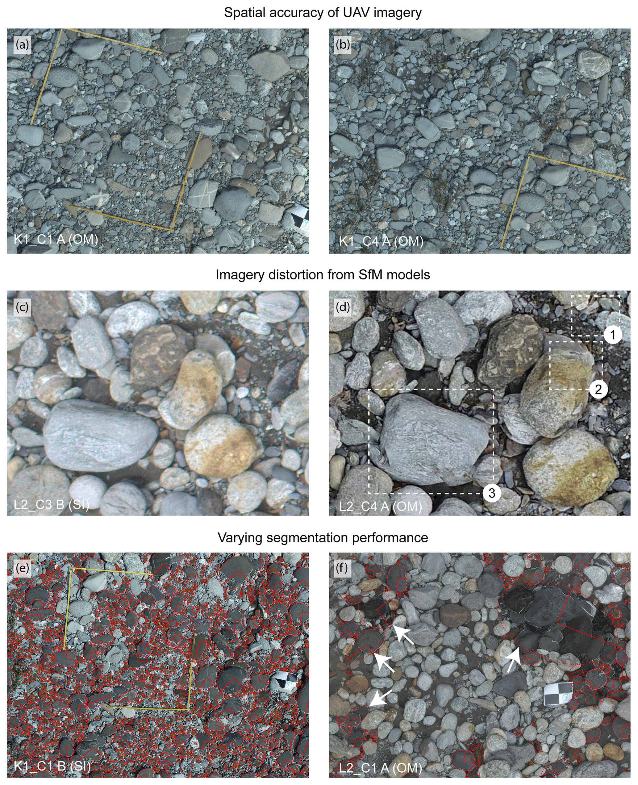
Figure 10 Systematic factors that influence grain size estimation from UAV imagery, especially from orthophoto mosaics (OM). (a, b) Effect of varying accuracy of SfM (structure from motion) used for referencing for orthophoto mosaics, which should display the same extent. (c, d) Comparison of undistorted single, nadir images (SI) with orthophoto mosaics, which highlight small-scale image warping and artifacts: (1) duplication from incorrect image stitching, (2) blurring of pebble boundaries, and (3) irregular grain shapes. (e, f) Selected results highlighting the varying image segmentation performance. Examples of systematic under-segmentation marked with white arrows.

4.5 Implications for workflows on grain size estimation

Our results have general implications for the estimation of grain sizes from UAV-acquired imagery. We will present these in the order of a typical workflow that is generally employed upon measuring grain size datasets with a UAV–SfM workflow (e.g., Fig. 3). For UAV surveys with a subsequent SfM processing, best practice to achieve the highest quality in SfM models (e.g., James et al., 2020; Eltner and Sofia, 2020; Sanz-Ablanedo et al., 2020) includes GCP referencing and in theory storage of the images in the raw format. However, in the field raw image acquisition is seldom realized because of its technical cost, such as lower survey velocity and the larger file size. Such conditions need significantly longer time for file storage and cause a multiplication of photogrammetric processing time and file size. Therefore, and in light of the possibility of reducing the systematic error through modeling from a suitable set of GCPs (see James et al., 2020), the use of pre-processed JPEG images might be sufficient for most applications targeting grain sizes. Furthermore, survey designs without GCPs might be acceptable for grain size estimation in cases where (i) a high-precision spatial allocation of the grains is not needed; and (ii) a correct image referencing and undistorting is possible, potentially by using a pre-calibrated camera model (see also Carbonneau et al., 2018). In such cases, we recommend measurements on single, undistorted nadir images, especially when grain size distributions are expected to vary and sampling is done only locally. All these recommendations are valid independent of the method for grain size estimation.

In principle, using a segmentation approach for grain size estimation allows for rigorous error and uncertainty modeling. Specifically, SfM model uncertainties can be used for a statistically robust estimation of errors on grain datasets by combining a bootstrapping and Monte Carlo approach, as accomplished in this work. Even more, an error estimation can be accomplished for models without GCPs, for the case where a simple parametrization that is only based on a length and scale error is considered (see supporting Code S1). We emphasize that this is only possible when the image distance can be estimated. We also note that this approach allows the estimation of uncertainties for datasets where grains were measured in other imagery, e.g., images acquired with a handheld camera. Generally, this approach returns uncertainty values for both measurement results and statistical processing, which includes effects related to counting statistics. To our knowledge, no such possibility for the estimation of uncertainties exists for grain size estimations that are based on statistical image parameters. However, current segmentation techniques are prone to biases that result from under- or over-segmentation and 2D projection effects of 3D structures. Therefore, in such cases, reduction in inaccuracies might be achieved through manual filtering of grains during segmentation (e.g., Purinton and Bookhagen, 2019; Detert and Weitbrecht, 2012) and/or through a calibration of the measurements with a reference dataset (e.g., Chardon et al., 2022), where data were collected in the field, as exemplified in this work. Such a strategy is likely to improve the accuracy of grain size data and yields in an estimate of the related uncertainty.

5 Conclusions

Our field-based approach in combination with the simple uncertainty modeling can be used to model all relevant uncertainties in SfM models onto grain size data that are extracted from segmented UAV imagery. The workflow proposed in this paper is applicable to any tasks that aim at measuring grain size data from images, and it allows us to assess the sensitivity of such grain size data on the UAV survey strategy. This includes selection of the image acquisition format, for which the use of the raw image format during image acquisition instead of the JPEG format might reduce the systematic uncertainty in topographic models. For our setup, the image format used for grain size estimation was a key variable, where an overall higher precision and accuracy were achieved if grain sizes were measured in single, undistorted nadir images rather than on orthophoto mosaics. Furthermore, general UAV survey conditions, e.g., light, wind, or vegetation exert a control on the precision and accuracy of grain size data estimated from images, even if the topographic models used for referencing are of high quality. Contrarily, our grain size data are not very sensitive to the quality of the topographic model, as long as single, undistorted nadir images are used where distortions were corrected with a camera lens model during the photogrammetric processing.