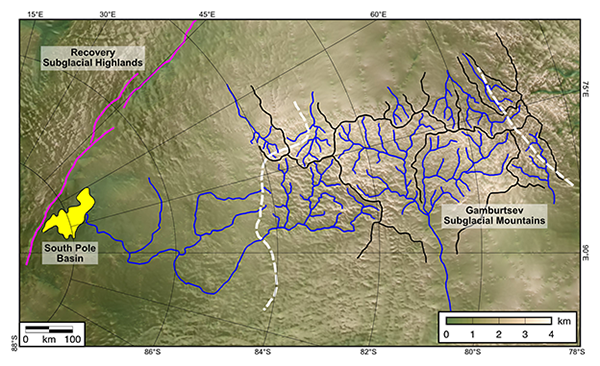
Valley longitudinal profiles record the fluvial landscape evolution and geological structure of the Gamburtsev Subglacial Mountains, East Antarctica

Fluvial valley networks in mountain ranges record the interactions between climate, tectonics, and lithology. While drainage network analysis has transformed our understanding of these interactions in subaerial settings, the landscape evolution of ice-covered orogens is poorly known. The Gamburtsev Subglacial Mountains are a ∼ 600 km-long mountain range situated beneath the East Antarctic Ice Sheet. These mountains were an important nucleation site for the ice sheet approximately 34 million years ago and are now buried beneath ∼ 2 km of ice. Airborne radar surveying has revealed that the Gamburtsevs are characterised by a rugged, incised landscape, but their geological structure and uplift history remain enigmatic. Here we use a compilation of radar survey data to extract and quantify valley longitudinal profiles from the Gamburtsevs and in turn infer details of their tectonic and geomorphic development. We use χ-mapping and stream power incision modelling to show that valley network morphology is consistent with a fluvial landscape that was locally overprinted by early mountain glaciation. The spatial distribution of channel steepness indices allows us to determine the position of major geological boundaries at the edges of the mountains. We also use independent estimates of denudation rates to evaluate competing scenarios for the timing of mountain uplift and valley incision, finding that uplift of the modern Gamburtsevs most likely commenced in the Mesozoic or early Cenozoic. Regional geomorphic analysis suggests that base level for some Gamburtsev fluvial catchments was set by enclosed interior basins associated with extensional faulting. These depocentres may retain detrital sedimentary material eroded from the Gamburtsevs prior to Antarctic glaciation and are potential targets for future sub-ice drilling campaigns.

1 Introduction

The East Antarctic Ice Sheet (EAIS) is the largest ice mass on Earth, with a volume of ∼ 24 million km³ and a sea-level equivalent of ∼ 52 m (Pritchard et al., 2025). The EAIS dates back to ca. 34 million years ago (Ma), when a protracted decline in atmospheric CO₂ and global temperatures (Hönisch et al., 2023; Westerhold et al., 2020) reached a threshold that triggered rapid East Antarctic glaciation (DeConto and Pollard, 2003). A positive feedback of increasing ice-surface elevation and mass balance, increasing surface albedo, and decreasing surface temperatures enabled a rapid transition from late Eocene mountain glaciers and ice fields to an early Oligocene continental-scale ice sheet with margins reaching the coast (Coxall et al., 2005; Gulick et al., 2017; Jamieson et al., 2010).

The EAIS likely nucleated on regions of high topography, including Dronning Maud Land, the Gamburtsev Subglacial Mountains (GSM), and the Transantarctic Mountains (DeConto and Pollard, 2003; Jamieson et al., 2010), all of which have peaks > 3 km above sea level (Pritchard et al., 2025). Uniquely among these regions, the GSM are entirely covered by the EAIS, with no surface outcrop. The GSM are situated beneath Dome A, the highest point on the EAIS (Fig. 1a). Their topography (Fig. 1b) has been partially surveyed using radio-echo sounding (Bell et al., 2011; Ferraccioli et al., 2011), which has revealed a landscape characterised by sharp ridges and steep-sided valleys with up to 1 km of valley-scale relief (Bo et al., 2009; Rose et al., 2013).

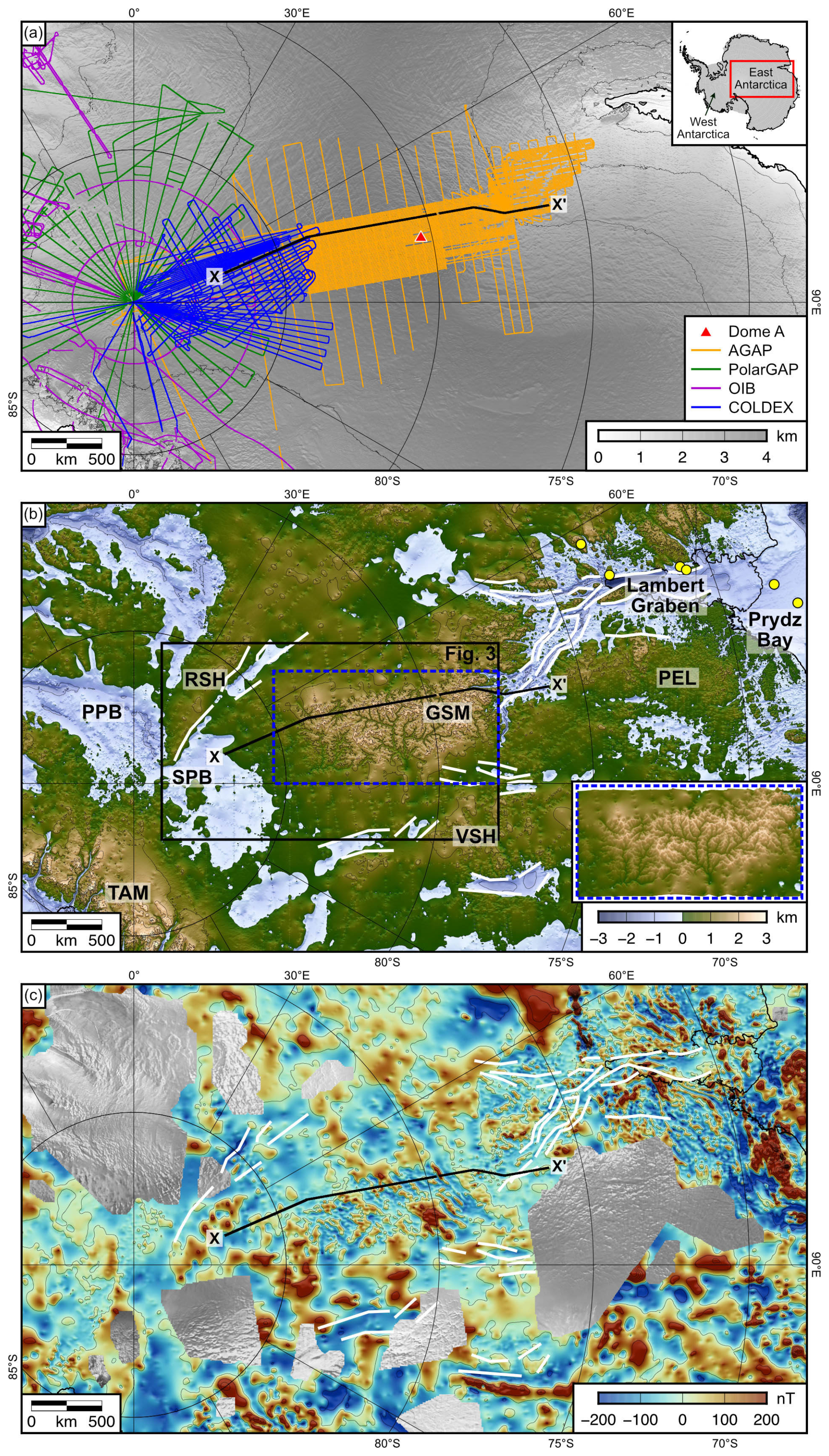
Figure 1 Regional setting of the Gamburtsev Subglacial Mountains. (a) Airborne radio-echo sounding surveys used in this study, overlain on hillshaded surface elevation from the Reference Elevation Model of Antarctica (contour interval = 1 km) (Howat et al., 2019). Thick black line marks the grounding line (MEaSUREs version 2). Inset shows the study area within East Antarctica. (b) Bed elevation relative to mean sea level from Bedmap3 (contour interval = 1 km) (Pritchard et al., 2025). Profile X–X^′ is displayed in Fig. 2; box shows the extent of Fig. 3. White lines mark the East Antarctic Rift System (Ferraccioli et al., 2011). Yellow circles mark offshore sediment core and onshore moraine locations where samples have been collected for detrital thermochronological analysis (Thomson et al., 2013). Abbreviations: GSM = Gamburtsev Subglacial Mountains; PEL = Princess Elizabeth Land; PPB = Pensacola-Pole Basin; RSH = Recovery Subglacial Highlands; SPB = South Pole Basin; TAM = Transantarctic Mountains; VSH = Vostok Subglacial Highlands. Inset shows a perspective image of the Gamburtsevs (covering the dashed blue area). The topography is viewed from an azimuth of 180° and an angle of 70°, with ∼ 20× vertical exaggeration. (c) ADMAP-2B magnetic anomaly compilation (contour interval = 200 nT) (Eagles et al., 2024; Golynsky et al., 2018). Data gaps are filled by the RADARSAT RAMP AMM-1 SAR image mosaic version 2 (Jezek et al., 2013).

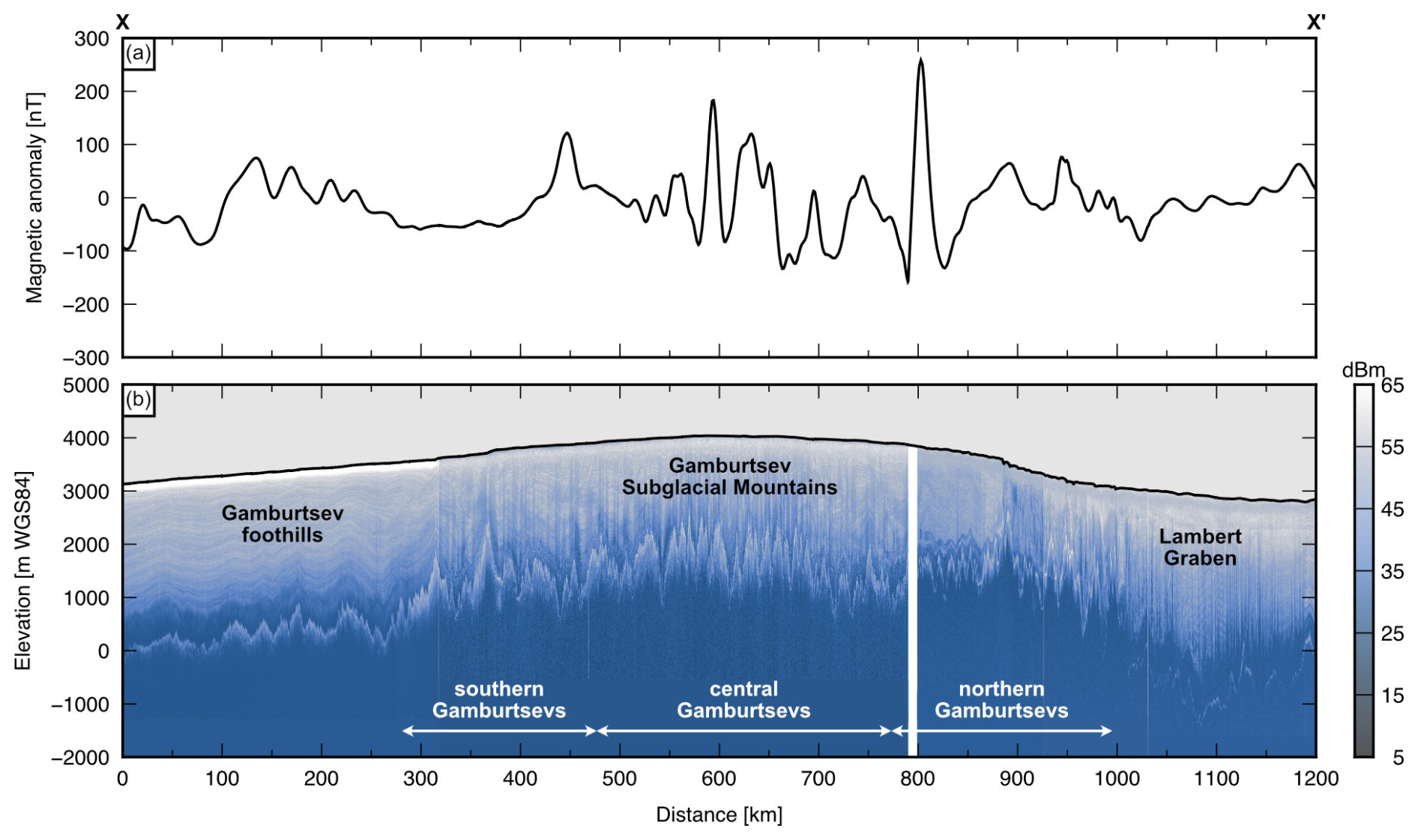
Figure 2 Cross-section of the Gamburtsev Subglacial Mountains. Location of profile X–X^′ is shown in Fig. 1. (a) Magnetic anomaly sampled from the ADMAP-2B compilation (Eagles et al., 2024; Golynsky et al., 2018). (b) Depth-corrected radargram across the Gamburtsevs with ∼ 50× vertical exaggeration. Black line marks the ice surface; elevations are relative to the WGS84 ellipsoid. Colour scale represents the power of the radar return (in decibel-milliwatts); vertical white line at ∼ 800 profile-km is a data gap.

Geomorphic analysis of the GSM has revealed evidence for partial erosive modification of a fluvial landscape by local-scale, warm-based glaciation, although the original fluvial planform organisation has been retained (Creyts et al., 2014; Rose et al., 2013). Mapping of landforms including cirques, overdeepenings, U-shaped valleys, and drainage divide breaches was used to demonstrate that early GSM glaciation was local in pattern, restricted to high-elevation ice fields at, or prior to, ca. 34 Ma (Rose et al., 2013). There are two further lines of evidence to suggest that glacial erosive modification of the GSM landscape primarily occurred prior to continental ice-sheet expansion at ca. 34 Ma and not during subsequent retreat intervals. First, global sea-level reconstructions show that ice-volume fluctuations through the Oligocene and Neogene were not sufficiently large to signify that, at any stage after ca. 34 Ma, ice was confined to small, local ice fields on the highest terrain (Miller et al., 2024; Rohling et al., 2022). Second, ice-sheet modelling suggests that cold-based ice was established over the GSM as soon as the EAIS expanded beyond a locally-glaciated system at ca. 34 Ma and that this cold-based, non-erosive core persisted over the GSM throughout the Oligocene and Neogene (Jamieson et al., 2010). This preservation of the GSM landscape enables quantitative analysis of the geomorphic record of fluvial landscape development and early mountain-scale glaciation.

The GSM are flanked to their north, east, and west by basins of the East Antarctic Rift System (Fig. 1b), a continental rift system that is hypothesised to have formed as a result of Permo-Triassic (ca. 300–250 Ma) extension and reactivated during a phase of Cretaceous (ca. 100 Ma) transtensional deformation (Ferraccioli et al., 2011; Phillips and Läufer, 2009). The rift system exhibits low-magnitude (M_w 2–4) seismicity today (Lough et al., 2018). To the south of the GSM is the South Pole Basin (SPB); the western side of the SPB is bounded by the southern end of the Recovery Subglacial Highlands (RSH; Fig. 1b) (Paxman et al., 2019; Young et al., 2025).

Multiple mechanisms have been hypothesised to explain the origin of the GSM, including collisional orogeny, rift-induced uplift, mantle plume activity, and erosionally-driven uplift (An et al., 2015; Ferraccioli et al., 2011; Paxman et al., 2016; Sleep, 2006; Van De Flierdt et al., 2008; Veevers et al., 2008). However, the absence of in situ bedrock samples from the GSM means the geological structure and evolution of the landscape prior to glaciation are poorly understood, with tectonic interpretations relying largely on gravity and magnetic surveying (Ferraccioli et al., 2011) (cf. Fig. 1c). Fundamental questions about the GSM remain unanswered, including their lithological composition, the tectonic and surface processes that have shaped their topography, and the timing of relief generation. There is a need to resolve these unknowns as they will have directly influenced the climatic threshold for EAIS nucleation, early ice-flow directions and thickness patterns, and the pace of the transition from mountain glaciation to continental-scale ice coverage (DeConto and Pollard, 2003; Jamieson et al., 2010; Rose et al., 2013), all of which remain poorly understood.

The well-imaged valley network within the Gamburtsevs (Fig. 1b) offers a valuable opportunity to address these questions, particularly if elements of the pre-glacial fluvial network are well preserved (Creyts et al., 2014; Rose et al., 2013). Fluvial valley networks are ubiquitous in subaerial mountain ranges and evolve in response to the balance between rock uplift and erosion (Howard, 1994). Analysis of their planform networks and longitudinal profiles has transformed our understanding of the tectonic and topographic evolution of those areas (Lague, 2014; Whipple and Tucker, 1999). For example, the morphology of river longitudinal profiles, including their steepness and concavity, has been used to quantify spatiotemporal variations in tectonic rock uplift rate, climate and erosion rates, and lithology (Duvall et al., 2004; Goren et al., 2014; Wobus et al., 2006). However, this approach has not been applied to a subglacial mountain range.

The aim of this study is to understand the tectonic and fluvial controls on the topographic evolution of the Gamburtsevs via analysis of valley longitudinal profiles. The objectives of this analysis are to:

• 1.

  Constrain the geological structure of the GSM;

• 2.

  Ascertain whether the GSM exhibit a steady-state or transient fluvial landscape and place constraints on its age;

• 3.

  Examine the influence of regional tectonics on base level and sediment routing; and

• 4.

  Assess the degree to which the fluvial landscape was modified by early mountain glaciation.

2 Geophysical Data

2.1 Radio-echo sounding

For this study, we used bed elevation measurements derived from four airborne radio-echo sounding (RES) surveys (Fig. 1a), with details on survey instrumentation provided in the references listed:

• AGAP (Antarctica's Gamburtsev Province) 2007/08 (Bell et al., 2011; Ferraccioli et al., 2011)

• PolarGAP 2015/16 (Paxman et al., 2019; Winter et al., 2018)

• Operation IceBridge 2010, 2014, 2016, 2017, and 2018 (MacGregor et al., 2021)

• COLDEX (Centre for Oldest Ice Exploration) 2022/23 and 2023/24 (Young et al., 2025)

All surveys determined ice thickness along flight tracks by calculating the two-way travel time of radar reflections at the ice surface and bed interfaces and assuming a uniform radio wave velocity (see the Supplement). Bed elevation (relative to the WGS84 ellipsoid) was computed by subtracting the ice thickness from the surface elevation (as measured by the survey). Positional data (latitude, longitude, and height referenced to the WGS84 ellipsoid) were recorded using dual-frequency GPS with an absolute accuracy of < 1 m. Although the surveys employed different radar platforms (see the Supplement), the centre frequencies and processing steps were similar, and each survey had an along-track trace spacing (horizontal sampling rate) of 15–30 m and a vertical resolution of ∼ 10 m.

Together, these surveys (Fig. 1a) have excellent coverage of the core massif of the GSM, along with the Lambert Graben to the north, the Gamburtsev foothills to the south, and the SPB and RSH (Figs. 1b and 2). In these regions of relatively dense RES coverage, flight line spacing is ∼ 5 km. However, coverage to the east and west of the GSM is limited to a small number of widely spaced (∼ 66 km) AGAP reconnaissance lines, making the subglacial topography difficult to resolve in these areas (Fig. 1a and b). We transformed geographic (latitude and longitude) positional data into x/y co-ordinate pairs in the EPSG:3031 WGS84/Antarctic Polar Stereographic projection and shifted all ice surface and bed elevation values onto the EIGEN-GL04C geoid (i.e., mean sea level) to ensure consistency with the Bedmap3 continental DEM (Pritchard et al., 2025).

2.2 Magnetic anomalies

To aid interpretations of subglacial geological structure, we used ADMAP-2B, the most recent compilation of magnetic anomalies for the Antarctic (Eagles et al., 2024; Golynsky et al., 2018). The ADMAP-2B compilation contains near-surface (primarily airborne and shipborne) magnetic anomaly data south of 60° S gridded at an interval of 1.5 km and low-pass filtered for wavelengths > 7 km (Fig. 1c). Some gaps in the vicinity of the South Pole have been partially filled by data acquired since the publication of ADMAP-2B (Frémand et al., 2022). However, the ADMAP-2B coverage over the Gamburtsev region is sufficient for the purposes of this study without needing to incorporate additional data from the peripheral regions. Our aim was to identify changes in the intensity and structural pattern of the magnetic anomalies (e.g., Fig. 2) that may reflect the presence of major geological boundaries beneath the ice sheet.

3 Methods

3.1 Valley longitudinal profile extraction

The approximate locations of the valleys within the Gamburtsevs can be identified by visual inspection of the Bedmap3 DEM (Fig. 1b), which we used to guide a systematic search of RES lines. We extracted the (x,y) co-ordinates and bed elevation (relative to the EIGEN-GL04C geoid) of valley floors (the lowest measured bed elevation within the valley) from the RES profiles that intersect the valleys. Since we were primarily interested in valley incision prior to ice-sheet growth, bed elevations were isostatically adjusted to account for the unloading of the Antarctic Ice Sheet. To do so, we used a model for the isostatic response to complete deglaciation (Paxman et al., 2022) updated for the Bedmap3 ice load (Pritchard et al., 2025). For the purposes of subsequent hydrological analysis (Sect. 3.2), we also generated a rebounded version of the Bedmap3 DEM (Pritchard et al., 2025) (Fig. 3) using the same approach, with a horizontal resolution of 500 m. No adjustment was made for post-34 Ma erosional modification of the valley floors; we examine the impact of this process in Sect. 5.1.

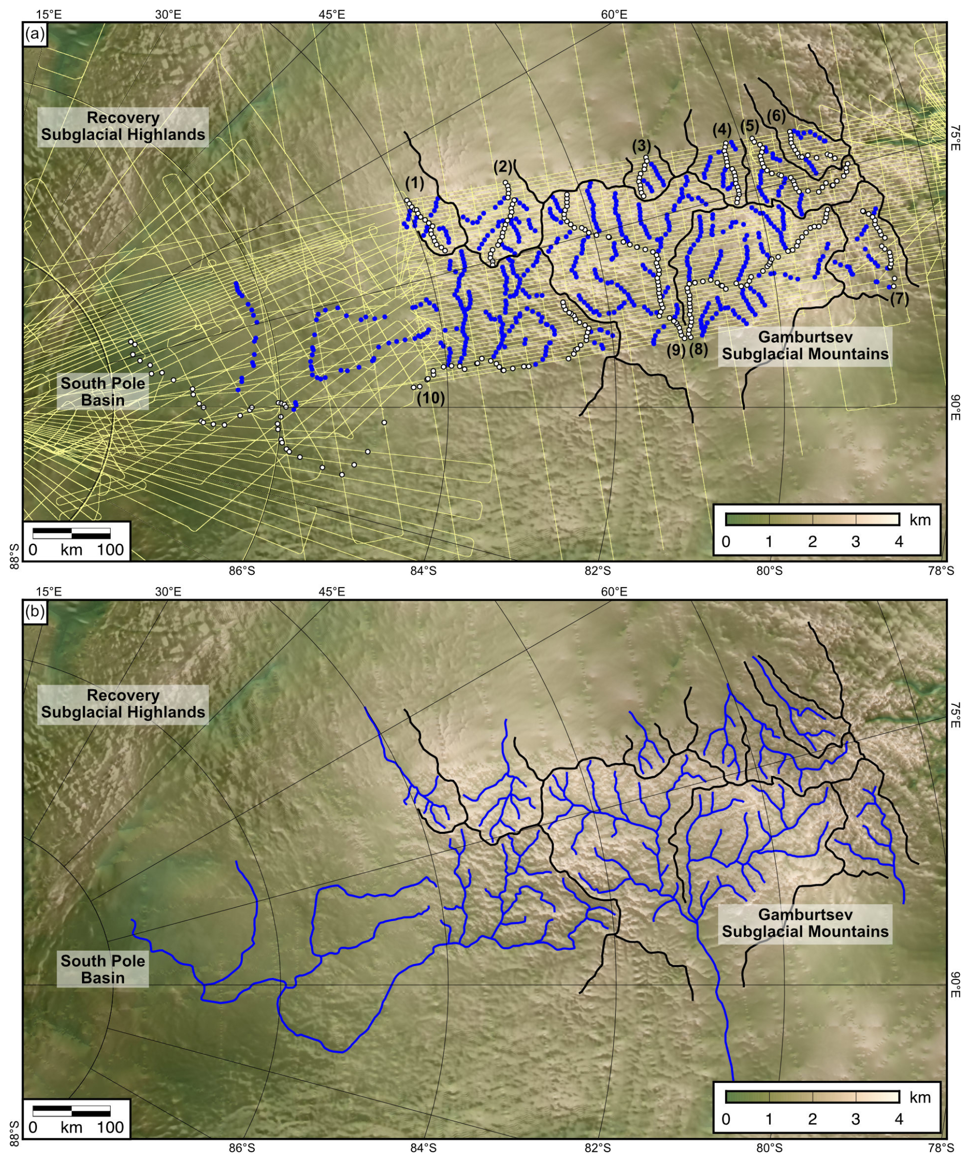
Figure 3 Valley networks in the GSM. (a) Locations of valley floors identified in RES-derived bed elevation data (survey coverage shown in yellow). The mapped valleys are organised into 10 basins (numbered with black lines marking drainage divides). Circles denote RES measurement points on the trunk (white) and tributary (blue) valleys. (b) Valley planform network (blue lines) derived from RES measurements and hydrological flow routing. For visualisation, some valleys are extrapolated further downslope beyond the lowermost RES point. The underlying bed elevation map is derived from Bedmap3 (Pritchard et al., 2025), isostatically rebounded for ice-sheet removal (Paxman et al., 2022). Shading is from the RADARSAT RAMP AMM-1 SAR image mosaic version 2 (Jezek et al., 2013).

Due to the limited spatial extent of the RES surveys, valley identification was primarily confined to the main AGAP survey grid, except for the well-surveyed area between 84 and 88° S that contains lines from all four RES surveys (Fig. 3a). In total, we identified 937 individual valley floor locations (Fig. 3a). The valleys were organised into 10 basins, each characterised by a trunk valley (defined as the longest continuous pathway) and tributaries. We mapped two orders of tributary upstream of the trunk valley; lower order headwater channels were not mapped as they were not consistently visible at the resolution of the RES data.

We then connected the RES point measurements to generate a two-dimensional planform network (Fig. 3b). This was guided by computing the hydrological drainage network for the rebounded Bedmap3 DEM. The DEM was filled to remove hydrological sinks, and the flow direction was determined assuming water is routed downslope from each pixel to its lowest neighbour (using a D8 algorithm). This approach assumes that there has been negligible valley erosion by subglacial meltwater, which is supported by the presence of cold-based ice over the GSM (Seiner et al., 2025) and the inference that where any localised meltwater in the valleys is pushed uphill, it encounters colder ice and refreezes to the bed, facilitating landscape preservation rather than erosion (Creyts et al., 2014). We then computed the upstream area for each grid cell (i.e., the flow accumulation) and extracted a hydrological network assuming an upstream area threshold for channel initiation of 50 km² (200 cells; Fig. S1 in the Supplement), which we found produced a network of similar resolution to that which was mappable using RES data. These calculations were performed using TopoToolbox version 3 (Schwanghart and Scherler, 2014). For each basin, we constructed longitudinal profiles (upstream distance vs. elevation) for the trunk valley and all tributaries. Only elevations derived from RES point measurements were used to construct these profiles (i.e., elevations were not interpolated between RES lines). The planform network was used to calculate along-profile distance, upstream drainage area, and to differentiate between trunk and tributary valleys. Along-profile distance was set to zero at the first (i.e., furthest downslope) RES-derived point on the trunk valley and increased moving upslope along the thalwegs (Fig. 3b).

To assess the extent of modification of fluvial valley systems by early mountain glaciation across the GSM, and thus ascertain which drainage basins are most amenable to the analyses described in Sect. 3.2 and 3.3, we compared the extracted longitudinal profiles to a set of criteria that may indicate fluvial erosion vs. glacial modification. Specifically, fluvial profiles are expected to exhibit smoothly graded, concave-up shapes, both in the trunk valley and its tributaries. By contrast, glacially-modified profiles may exhibit steepened “headwaters”, enclosed lows (“overdeepenings”), steps, and hanging valleys (Anderson et al., 2006; Deal and Prasicek, 2021; Lloyd et al., 2023). The analysis described in Sect. 3.2 also allows us to assess the degree to which the longitudinal profiles reflect fluvial vs. glacial erosion.

3.2 χ analysis

We aimed to quantify the shape of valley longitudinal profiles in the GSM (i.e., the relationship between channel slope and upstream drainage area), allowing us to identify spatiotemporal variations in fluvial erosion and/or uplift rate, whether the landscape is in steady state or shows evidence of transience, and signatures of valley modification by glacial erosion.

Assuming purely fluvial conditions, the slope of a river channel (S) at any point is a power law function of the upstream drainage area (A) (Flint, 1974):

$$\begin{array}{}\text{(1)}& S=k_{\mathrm{s}}{A}^{-\mathit{\theta }}\end{array}$$

where k_s is the channel steepness index and θ is the concavity index.

Expressions for k_s and θ can be derived from the stream power incision model (Howard and Kerby, 1983; Whipple and Tucker, 1999), which states that the erosion rate (E) of a river at any point is proportional to the upstream area (A) and slope (S):

$$\begin{array}{}\text{(2)}& E=K{A}^m{S}^n\end{array}$$

where m and n are positive exponents and K is the erodibility coefficient, which reflects a combination of factors that control erosional efficacy, including bed erodibility, river erosivity, sediment flux characteristics, and hydraulic geometry (Lague, 2014; Whipple and Tucker, 1999). At any point along the profile, the change in elevation (z) with time (t) is given by the difference between the rates of rock uplift (U) and erosion (E):

$$\begin{array}{}\text{(3)}& {\displaystyle \frac{\mathrm{d}z}{\mathrm{d}t}}=U-E\end{array}$$

If a river profile is in steady state ($\mathrm{d}z/\mathrm{d}t$ = 0), we can set U = E and rearrange Eq. (2) to form:

$$\begin{array}{}\text{(4)}& S={\left({\displaystyle \frac{U}{K}}\right)}^{\mathrm{1}/n}{A}^{-m/n}\end{array}$$

From comparison with Eq. (1), we can see that:

$$\begin{array}{}\text{(5)}& {\displaystyle }& {\displaystyle }\mathit{\theta }={\displaystyle \frac{m}{n}}\text{(6)}& {\displaystyle }& {\displaystyle }{k}_{\mathrm{s}}={\left({\displaystyle \frac{U}{K}}\right)}^{\mathrm{1}/n}\end{array}$$

These two indices define the shape of a river's longitudinal profile (i.e., how channel gradient changes as a function of drainage area). Moreover, since θ is given by the ratio of m and n, and k_s depends on U and K, these indices enable us to extract information pertaining to the tectonic and geological controls on landscape development (Wobus et al., 2006).

To constrain θ and k_s in the GSM, we used the integral approach (χ analysis) (Mudd et al., 2014; Perron and Royden, 2013). We rewrite the slope-area equation as:

$$\begin{array}{}\text{(7)}& {\displaystyle \frac{\mathrm{d}z}{\mathrm{d}x}}=k_{\mathrm{s}}{A}^{-m/n}\end{array}$$

and integrate both sides upstream from base level (x_b)

$$\begin{array}{}\text{(8)}& \underset{z\left(x_{\mathrm{b}}\right)}{\overset{z}{\int }}\mathrm{d}z=\underset{x_{\mathrm{b}}}{\overset{x}{\int }}{k}_{\mathrm{s}}{A}^{-m/n}\mathrm{d}x\end{array}$$

which gives

$$\begin{array}{}\text{(9)}& z\left(x\right)=z\left(x_{\mathrm{b}}\right)+\left({\displaystyle \frac{k_{\mathrm{s}}}{A_{\mathrm{0}}^{m/n}}}\right)\mathit{\chi }\end{array}$$

where

$$\begin{array}{}\text{(10)}& \mathit{\chi }=\underset{x_{\mathrm{b}}}{\overset{x}{\int }}{\left({\displaystyle \frac{A_{\mathrm{0}}}{A\left(x\right)}}\right)}^{m/n}\mathrm{d}x\end{array}$$

x is the along-profile distance and A₀ is a reference area introduced to ensure the integrand is dimensionless. We used a standard value of A₀ = 10⁶ m² in all calculations, but the choice is immaterial to the results.

If a fluvial network is in steady state (U = E) and the uplift rate (U) and erodibility coefficient (K) are uniform in space and time, there should be a single linear relationship between χ and elevation when an appropriate value of θ ($m/n$) is used. Moreover, tributaries should be collinear with the trunk valley and with each other at the appropriate θ value (Mudd et al., 2014). Since the gradient of the straight line is proportional to k_s (Eq. 9), the χ-elevation plot allows us to independently constrain both θ and k_s. Deviations from a straight line may evidence (a) transient (non-steady-state) evolution of the profile (U ≠ E), (b) spatial/temporal variations in uplift rate or bedrock erodibility, or (c) modification by glacial erosion (Goren et al., 2014; Perron and Royden, 2013).

We computed χ using the hydrological network determined in Sect. 3.1 and integrating the drainage area in the upstream direction according to Eq. (10) (Fig. S1) using TopoToolbox version 3 (Schwanghart and Scherler, 2014). We extracted the χ value at each of the 937 RES measurement points on the valley network, and plotted this against rebounded (i.e., ice-free) bed elevation. It is important to note that the drainage network and χ were calculated for a rectangular area of the rebounded Bedmap3 DEM (Fig. S1), such that each basin does not start at the same base level (z(xb)) and χ values cannot be directly compared between basins. This is because the RES data coverage does not allow us to map most valley networks down to their true base level. However, our analysis focussed solely on the relative changes in χ and channel steepness within each basin, which are independent of the assumed base level.

To determine the best-fitting value of θ for each basin, we calculated χ for θ values between 0 and 1. We then performed a linear least-squares regression of elevation against χ and computed the correlation coefficient (R). The value of θ that best linearises the χ-elevation plot will yield the highest R value. We also computed maximum likelihood estimator and disorder metrics (Hergarten et al., 2016; Mudd et al., 2018) to find the value of θ that best collinearised the trunk valley and tributaries (see the Supplement).

For the optimal value of θ, we multiplied the gradient of the χ-elevation regression by $A_{\mathrm{0}}^{m/n}$ to determine k_s (Eq. 9). However, because k_s covaries with θ (Eq. 9), it is not possible to directly compare channel steepness indices from drainage basins with different concavity indices. To isolate the influence of tectonics and lithology on valley profile morphology, it is therefore necessary to compute a normalised channel steepness index (k_sn) corresponding to a reference concavity index (θ_ref). For this study, we assumed a θ_ref of 0.55, which is the mean value across all basins in the Gamburtsevs (median = 0.54; see Table S1 in the Supplement). If there are sections of the channel profile with different k_sn values, it is not appropriate to fit a single line through the entire profile (Mudd et al., 2014). Where relevant, we separated the χ-elevation plot into segments where each is characterised by a distinct gradient (i.e., k_sn) (Smith et al., 2022).

3.3 Stream power incision modelling

By combining Eqs. (2) and (3), we can formulate a partial differential equation that describes the rate of change of river profile elevation through time:

$$\begin{array}{}\text{(11)}& {\displaystyle \frac{\partial z}{\partial t}}=U\left(t\right)-K{A}^m{\left({\displaystyle \frac{\partial z}{\partial x}}\right)}^n\end{array}$$

This equation is known as the stream power incision model (SPIM) (Whipple and Tucker, 1999) and is widely used to simulate the evolution of fluvial landscapes. We used this equation to forward model longitudinal profiles for the Gamburtsevs, in order to: (i) verify whether the shape of the longitudinal profiles is consistent with fluvial incision, and (ii) place limits on the age and uplift history of the landscape using a plausible parameter space constrained as far as possible by observations.

In the SPIM, the constants K, m, and n are interdependent and unique values cannot be retrieved from longitudinal profile modelling alone (Croissant and Braun, 2014). We therefore used the $m/n$ ratio (θ) constrained in Sect. 3.2 and made the common assumption that n = 1, meaning $m/n$ = m. We assessed the impact of alternative values of n (0.8–1.2) on our results. We then substituted E for U in Eq. (6) and rearranged to form:

$$\begin{array}{}\text{(12)}& K={\displaystyle \frac{E}{(k_{\mathrm{s}}{)}^n}}\end{array}$$

Equation (12) indicates that if we have constrained k_s (for a given $m/n$), we can back-calculate K if we have an estimate of the average erosion rate (E). However, there are no constraints for Gamburtsev pre-glacial erosion rates from sediment yields or cosmogenic nuclides, which are widely used elsewhere on Earth. Given this limitation, our aim was to run the SPIM for a plausible range of E values and thereby establish a range for the age of the GSM fluvial landscape.

Globally, after discounting highly tectonically active regions that are unrepresentative of interior East Antarctica, long-term denudation rates in fluvial basins range between ∼ 10 and ∼ 1000 m Myr⁻¹ (Koppes and Montgomery, 2009). The only East Antarctic evidence is derived from detrital thermochronological analysis of Cenozoic clastic sediments in Prydz Bay and nearby coastal moraines (Fig. 1b), which implies long-term catchment-averaged denudation rates of 10–20 m Myr⁻¹ between the Permo-Triassic (ca. 250 Ma) and the late Eocene (ca. 34 Ma) (Thomson et al., 2013). However, thermochronology data integrate a large source region including mountainous and low-relief landscapes (Taylor et al., 2004), so likely underestimate maximum erosion rates in the Gamburtsevs. Moreover, on a global scale, erosion rates of ∼ 10 m Myr⁻¹ are confined to catchments with low slopes and relief (Portenga and Bierman, 2011; Summerfield and Hulton, 1994), which are not consistent with the observed GSM topography. Therefore, the erosion rates recovered from thermochronology likely reflect a regional spatiotemporal average and will not equate to the elevated erosion rates within the high-slope, high-relief Gamburtsev region.

On the other hand, however, erosion rates of ∼ 1000 m Myr⁻¹ would likely overestimate the pre-glacial denudation rate for the Gamburtsevs. These values are typically associated with active mountain ranges in convergent tectonic settings with sub-tropical, monsoon-dominated climates, such as the Himalayas or Taiwan (Koppes and Montgomery, 2009). The presence of Nothofagus (southern beech) and conifers in the Antarctic Palaeogene fossil plant record implies a cool-temperate climate akin to modern-day Patagonia (Francis et al., 2008), and thus lower erosion rates. Tectonically, more appropriate analogues for the GSM may be less active extensional orogens such as the Italian Apennines or Basin and Range Province in the western USA; in these ranges, erosion rates are consistently on the order of 10s to 100s of m Myr⁻¹ (Densmore et al., 2009; Koppes and Montgomery, 2009). Moreover, sediment volumes in Prydz Bay do not show evidence for Himalayan- or Taiwan-level fluvial sedimentation rates (and thus onshore erosion rates) prior to East Antarctic glaciation (Cox et al., 2010; Jamieson et al., 2005).

An intermediate E value of 100 m Myr⁻¹ may therefore be the most appropriate for the GSM. This is supported by global analysis of river basins, which indicates that the relief ratio (relief/length) of a drainage basin is the strongest predictor of denudation rate (Summerfield and Hulton, 1994). The relief ratio of Gamburtsev basin 10 (containing the only thalweg whose mapped extent was not limited by RES data coverage; see Sect. 4.1) is 0.0028, which corresponds to a denudation rate of ∼ 50 m Myr⁻¹ (Fig. S2). In addition, maximum slopes in the GSM are ∼ 20° (∼ 400 m km⁻¹) (Rose et al., 2013). In global empirical compilations, these slopes correspond to a 50th percentile denudation rate of ∼ 100 m Myr⁻¹ and a 95th percentile of ∼ 500 m Myr⁻¹ in metamorphic rocks (Zondervan et al., 2023). We therefore proceeded using a most likely order of magnitude for E of 100 m Myr⁻¹ and performed sensitivity tests for the lower and upper limit scenarios of 10 and 1000 m Myr⁻¹, respectively. For these three values of E, we computed the corresponding K using the k_s and θ (with n = 1) recovered from χ analysis. We note that these values of E were used solely for back-calculating K. In our forward models, E is not set and evolves through time in response to U. Determining K in this way also assumes steady-state behaviour over these timescales.

To solve the SPIM, we used a total variation diminishing finite volume method, which is less sensitive to numerical smearing than other partial differential equation solvers and has been demonstrated to produce solutions consistent with analytical methods (Campforts et al., 2017; Campforts and Govers, 2015). The spatial domain of our models was the mapped length of the longitudinal profile. The horizontal resolution was 1 km and the time step was 1 Myr.

We performed two model experiments. First, we examined the simple case where we assumed that the uplift rate (U) was spatially and temporally uniform. We assumed the initial topography was a flat land surface with an elevation equal to that of lowest mapped point on the trunk valley (which acts as “base level” for SPIM purposes although most valleys will continue further downstream beyond the surveyed area). We set the maximum amount of uplift to match the elevation of the highest point on the longitudinal profile relative to this “base level” and tuned the model run time to best fit the observed profile for the assumed combination of m, n, and K. Second, we performed simulations where pulses of increased uplift rate (i.e., base-level fall) were introduced, leading to the generation of propagating knickpoints (see the Supplement). In this situation, the response time (τ_G) for perturbations to propagate upstream from base level (if n = 1) is expressed as (Whipple and Tucker, 1999):

$$\begin{array}{}\text{(13)}& {\mathit{\tau }}_{\mathrm{G}}\left(x\right)=\underset{\mathrm{0}}{\overset{x}{\int }}{\displaystyle \frac{\mathrm{1}}{KA(x{)}^m}}\mathrm{d}x\end{array}$$

The response time increases monotonically with x, such that channel reaches farther away from base level will have higher response times than lower channel reaches closer to base level.

3.4 Regional tectonics and base level

The dense RES survey line coverage between the Gamburtsev foothills and the SPB (Fig. 3a) provides an opportunity to assess the regional tectonic structure surrounding the GSM within the wider context of the East Antarctic Rift System (Fig. 1b). We focussed on the influence of regional tectonics on: (i) the base level to which valley networks within the GSM may have eroded, and (ii) the location of sediment depocentres within East Antarctica. To do so, we conducted a four-part topographic analysis.

First, we examined the root mean square (RMS) deviation of bed elevation along RES flight tracks over a 400 m length scale (Young et al., 2025), which is a proxy for large-scale roughness of the subglacial terrain. This may enable identification of e.g., smooth sediment-filled basins. Second, we traced linear features in the RADARSAT RAMP AMM-1 SAR image mosaic (Jezek et al., 2013), which reveals ice-surface undulations that correspond with regions of steep subglacial topography and may reflect tectonic structures such as faults (Chang et al., 2016). Third, we quantified the along-strike variation in elevation and half-width of the RSH, which can be used to constrain the direction and recency of fault propagation (Densmore et al., 2005, 2007). We sampled elevations from the rebounded Bedmap3 DEM along a swath of 20 profiles oriented parallel to the strike of the range front. RSH half-width was approximated as half the horizontal distance across the region enclosed by the 1500 m contour (under ice-free conditions). Fourth, we used an elastic plate model to compute the flexural response to mechanical unloading (due to extensional faulting) and erosional unloading to evaluate whether these two processes can account for the configuration of the regional topography, as would be expected in a continental rift system setting (Contreras-Reyes and Osses, 2010; Ebinger et al., 1991; Watts, 2023) (see the Supplement).

4 Results

4.1 Longitudinal profile morphology

Figure 4 shows the longitudinal profiles of the trunk valleys and their tributaries that we extracted from the 10 drainage basins identified in the GSM. The number of tributaries mapped per basin ranged between 2 and 18, with a total of 85 distinct valley thalwegs (10 trunks; 75 tributaries) across the 10 basins. The mapped length of the trunk valleys ranged from 54.3 km (basin 3) to 947 km (basin 10). The longitudinal profiles of basins 1–9 could only be mapped as far downslope as the edges of the AGAP survey grid (Fig. 3a), with a maximum trunk valley thalweg length of 314 km (basin 8). The highest (furthest upslope) points on the longitudinal profiles are currently situated at elevations of ∼ 1000–1500 m above sea level. However, isostatic adjustment for the removal of the EAIS would contribute ∼ 700 m of uplift across the Gamburtsevs (Paxman et al., 2022). Therefore, under ice-free conditions the upper reaches of the longitudinal profiles would be situated at ∼ 1700–2200 $\mathrm{m}\mathrm{a}.\mathrm{s}.\mathrm{l}.$ (Fig. 4). The lowermost mapped valley floors would be situated at ∼ 1000–1500 $\mathrm{m}\mathrm{a}.\mathrm{s}.\mathrm{l}.$ (Fig. 4). We also note that the upper reaches of the longitudinal profiles in the northern Gamburtsevs (basins 5, 6, and 7) appear to be characterised by gentler gradients than those in the central (3, 4, 8, and 9) and southern (1, 2, and 10) Gamburtsevs (Fig. 4).

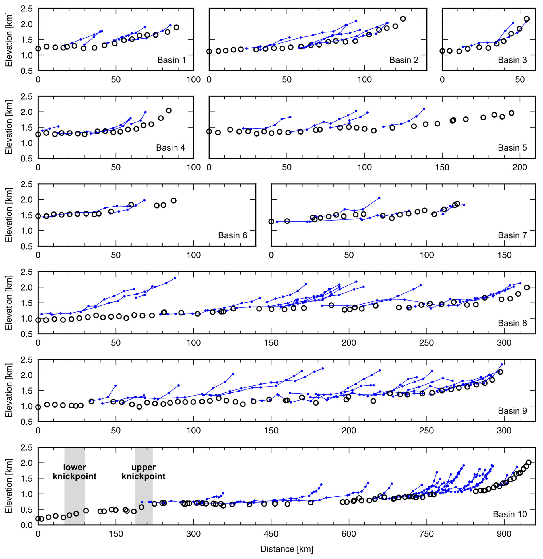
Figure 4 Longitudinal valley profiles for all basins in the GSM. Black circles = trunk valleys; blue circles/lines = tributaries. Elevations are relative to mean sea level and have been isostatically adjusted for the removal of the ice sheet (Paxman et al., 2022). Note that the horizontal scale is the same for each profile except basin 10. Shaded regions mark the knickpoints mentioned in the text.

The resolution of the RES data and density of measurements along the longitudinal profiles were sufficient to capture the morphology of the profiles at length scales appropriate for our analysis. Along-track bed elevation measurement spacings are 15–30 m and vertical resolutions are ∼ 10 m, which are well below the length-scale of our analysis (> 1000 m). The frequency distribution of the along-thalweg distance between adjacent RES measurements shows a strong modal peak at 5–6 km, reflecting the AGAP grid spacing (Fig. S3). We found that 87 % of point spacings are < 10 km and 98 % are < 20 km. Only 8 of the 852 point-spacings exceed 30 km, often occurring in gaps between survey grids or where the valley thalweg runs parallel to survey lines (Fig. 3). The spacing between RES lines means minor (order 100 m) elevation offsets at confluences between trunk valleys and tributaries may not be resolved. This means we cannot be certain whether any hanging valleys are present in the networks, although we note that no such features are definitively revealed by the available data (Fig. 4).

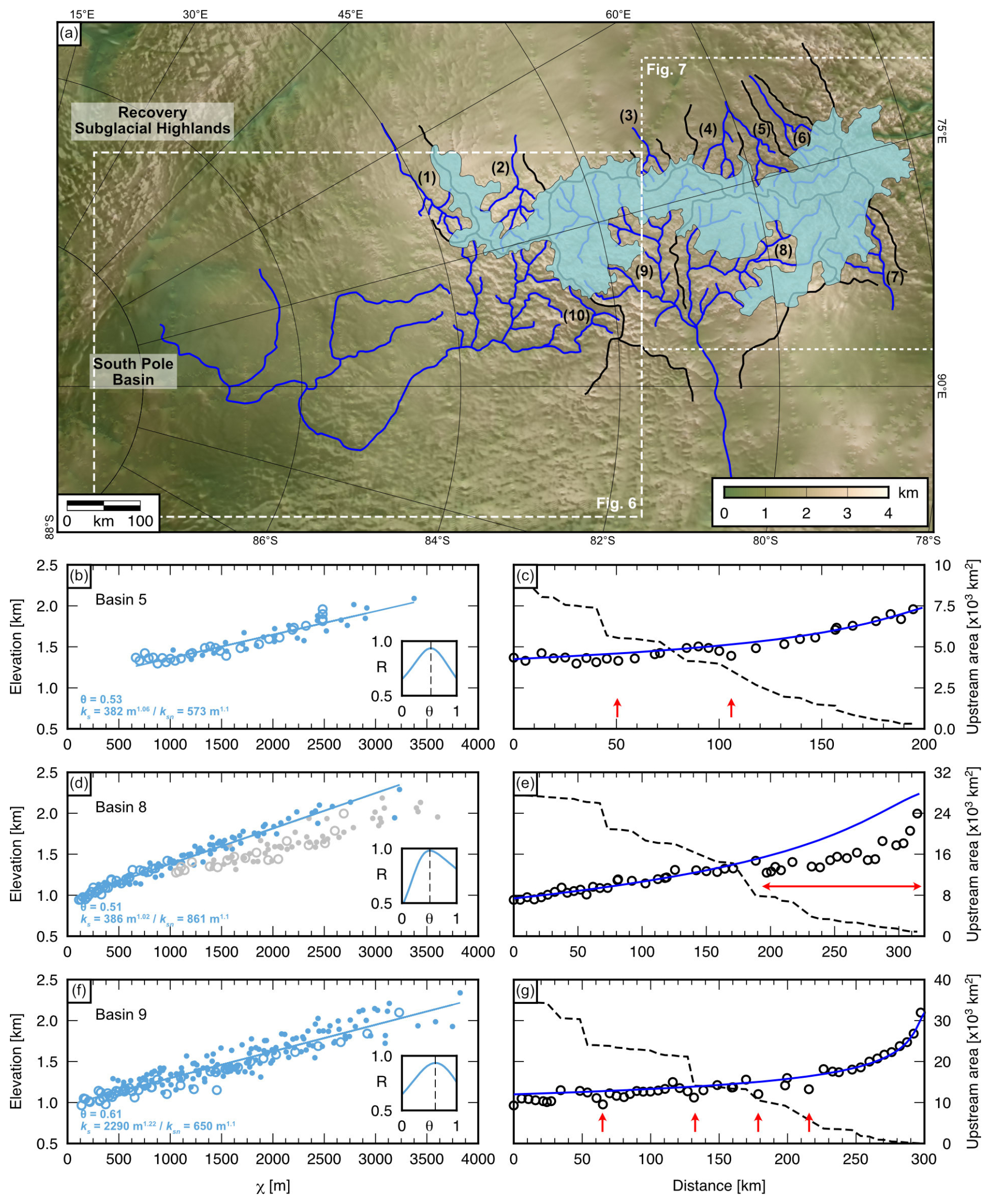
Figure 5 Relationship between Gamburtsev valley networks and mountain-scale glaciation at, or prior to, ca. 34 Ma. (a) Mapped GSM valley networks (blue lines) and drainage basin divides (black lines). Light blue shaded area marks the approximate mountain glacial limit at, or prior to, ca. 34 Ma, reconstructed using glacial geomorphological mapping (Rose et al., 2013). Bed elevations are derived from the rebounded Bedmap3 DEM (Paxman et al., 2022; Pritchard et al., 2025); shading is from the RADARSAT RAMP AMM-1 SAR image mosaic version 2 (Jezek et al., 2013). (b, d, f) χ-elevation plots for basins 5, 8, and 9, respectively. Open circles = trunk valleys; closed circles = tributaries. Best-fitting θ values are identified from the correlation coefficient (R; insets) of the linear regression (straight line). Recovered k_s and k_sn (θ_ref = 0.55) are labelled. (c, e, g) Corresponding theoretical fluvial longitudinal profiles calculated using Eq. (11) with the recovered θ and k_s (blue line), superimposed on the observed trunk profiles (circles). Dashed line denotes upstream drainage area. In panel (d), grey circles mark points that deviate from the linear part of the plot, corresponding to the section of the profile marked by the horizontal red arrow in panel (e). Vertical red arrows mark deviations below the theoretical fluvial profile (overdeepenings), which often correspond with step-increases in upstream drainage area (i.e., tributary junctions).

All trunk valley longitudinal profiles exhibit a concave-up morphology, with steeper channel gradients in the upper reaches and lower gradients further down. Tributaries are largely concave-up and smoothly and systematically join the trunk valleys in a downslope direction (Fig. 4). However, we note that not all longitudinal profiles decrease monotonically in elevation moving downslope; several valleys exhibit local minima (i.e., enclosed lows), which often coincide with tributary junctions (see e.g., basins 5, 7, and 9; Figs. 4 and 5). These localised deviations below the “expected” fluvial profile are up to ∼ 20 km long and ∼ 300 m deep. Some profiles also exhibit a “stepped” morphology (see e.g., basins 8 and 9; Fig. 5) and steepened “headwaters” (e.g., basin 8; Fig. 5). According to the criteria described in Sect. 3.1, these features suggest that parts of these drainage basins, which are situated in the higher-elevation central and northern GSM, have been locally modified by mountain glaciation.

RES survey coverage allowed us to map the longitudinal profile of basin 10 from the southern Gamburtsevs to the SPB. In contrast to basins in the central and northern GSM, features indicative of glacial erosion are not visible in this basin. As well as a well-defined concave-up form, this profile exhibits two ∼ 40 km-long regions of steeper channel gradient (i.e., knickpoints) that separate regions of shallower channel gradient (Fig. 4). The vertical relief (top-to-bottom elevation change) of the “lower” (situated at ∼ 90 profile-km) and “upper” (situated at ∼ 220 profile-km) knickpoints are ∼ 260 and ∼ 210 m, respectively (Fig. 4). Since it is the longest mapped longitudinal profile, shows minimal evidence of localised glacial modification, and is situated almost entirely outside of reconstructed early mountain glacial limits (Rose et al., 2013) (Fig. 5), we focussed our stream power incision modelling (Sect. 4.3) on basin 10.

4.2 χ-elevation relationships

Using χ-elevation plots, we were able to constrain θ and k_s for six of the 10 basins (2, 5, 7, 8, 9, and 10), which all yielded θ values that best linearised the χ-elevation plot of between 0.50 and 0.61 (Table S1). The maximum likelihood estimator and disorder metrics also found that the tributaries and the trunk valley were best collinearised in χ-elevation space by similar θ values (Fig. S4). However, the hydrological network and χ calculation in basins 1, 3, 4, and 6 were compromised by these comparatively small catchments being poorly resolved in the Bedmap3 DEM, partially owing to gridding artefacts, meaning a robust full-basin χ-elevation plot could not be constructed.

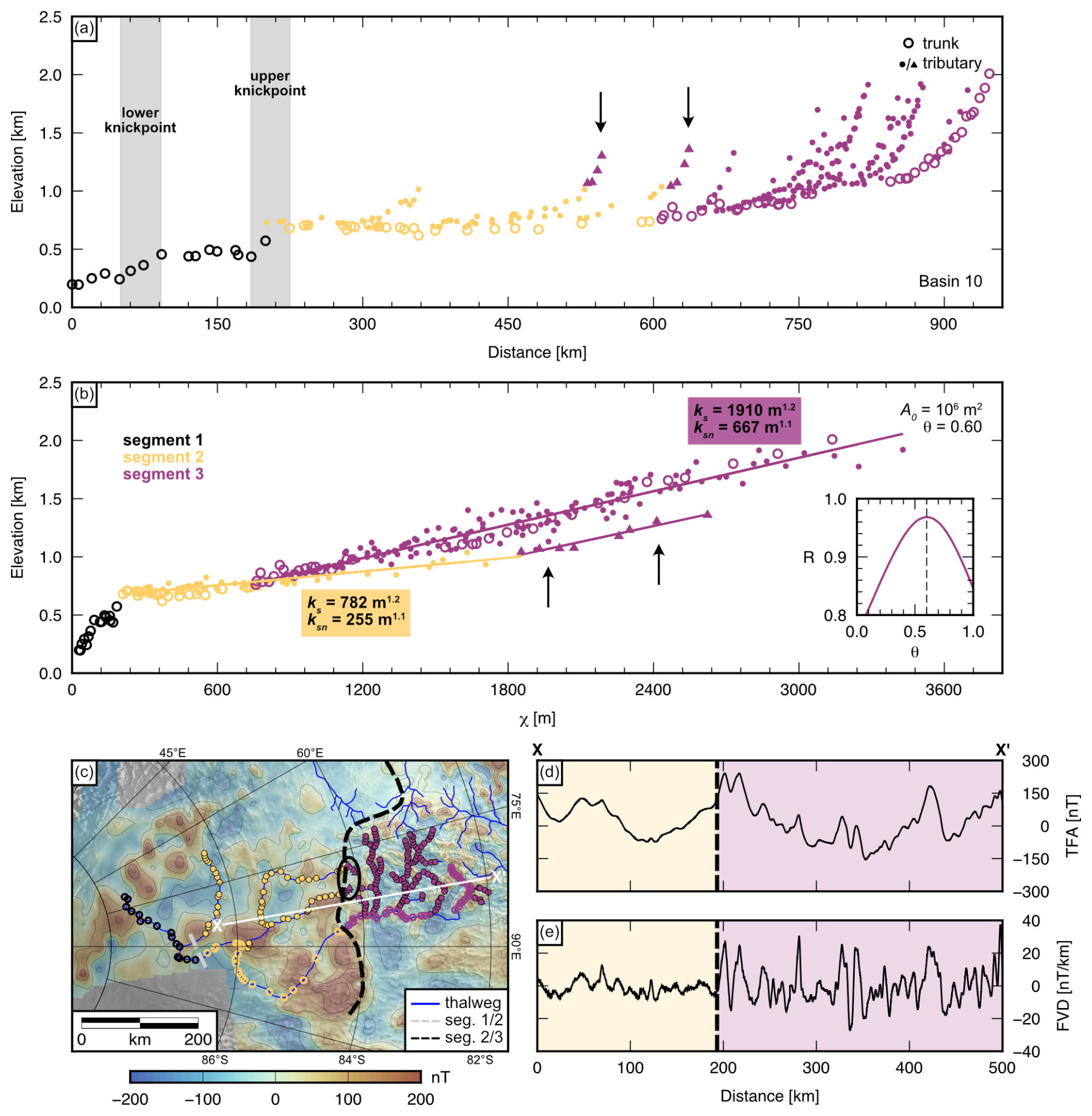
Figure 6 Longitudinal profile analysis in the southern GSM. (a) Longitudinal distance-elevation profile for basin 10. Colours denote segments of the profile in χ-elevation space. (b) χ-elevation plot, transformed with A₀ = 10⁶ m² and θ=0.60. The plot shows three linear segments with distinct gradients. Recovered values for k_s (for θ = 0.60) and k_sn (for θ_ref = 0.55) are labelled for the two segments above the knickpoints. Note that the upper reaches of two tributaries at approximately 84° S, 80° E (marked by triangle symbols and black arrows) are well fit by a separate regression line with a gradient equal to that of segment 3. Inset: correlation coefficient (R) as a function of θ for linear least-squares regression of segment 3. (c) Valley network overlain on the ADMAP-2B magnetic anomaly (Eagles et al., 2024; Golynsky et al., 2018). Boundaries between χ-elevation segments are marked. Black oval indicates the location of the tributaries marked in panels (a) and (b). Contour interval is 100 nT. Panel extent is shown in Fig. 5a. (d) Magnetic anomaly (total field anomaly; TFA) along profile X–X^′ (location shown in panel c). (e) First vertical derivative (FVD) of the TFA, which enhances the effects of shallow sources. The dashed vertical line marks the boundary between segments 2 and 3 (see panel c).

For basin 10, we visually identified three linear segments in χ-elevation space; segment 1 is downstream of the upper knickpoint (0–220 profile-km), segment 2 is between 220 and 600 profile-km, and segment 3 is above 600 profile-km (Fig. 6a and b). Segment 3, which contains 185 of the 278 RES measurement points in the basin, returned a best-fitting θ of 0.60 (via the R metric; Fig. 6b). The maximum likelihood estimator and disorder metrics indicated that the trunk valley and tributaries were best collinearised for θ values of 0.58 and 0.57, respectively (Fig. S4), showing that all three methods were in good agreement.

The boundary between segments 2 and 3 is marked by a step-change in k_s, with segment 2 having a value of 782 m^1.2 and segment 3 a value of 1910 m^1.2 (for θ = 0.60). The corresponding k_sn (θ_ref = 0.55) values are 255 and 667 m^1.1, respectively. We also found that the upper reaches of two tributaries situated between 520 and 640 profile-km were better fit by a regression line with a gradient equal to that of segment 3 (Fig. 6b and c). Although there is a degree of ambiguity over the exact position of the transition between segments 2 and 3 (Fig. 6b), visual segmentation is sufficient for identifying the approximate location of the boundary (Demoulin et al., 2015; Smith et al., 2022). Moreover, this approach can be validated through comparison with the magnetic anomaly. The boundary between segments 2 and 3 coincides with a marked change in the intensity and structural pattern of the magnetic anomaly. Segment 3 is characterised by short-wavelength (< 10 km) anomalies with vertical derivatives of up to ± 40 nT km⁻¹, whereas the short-wavelength signal is notably muted in segment 2 (Fig. 6c–e).

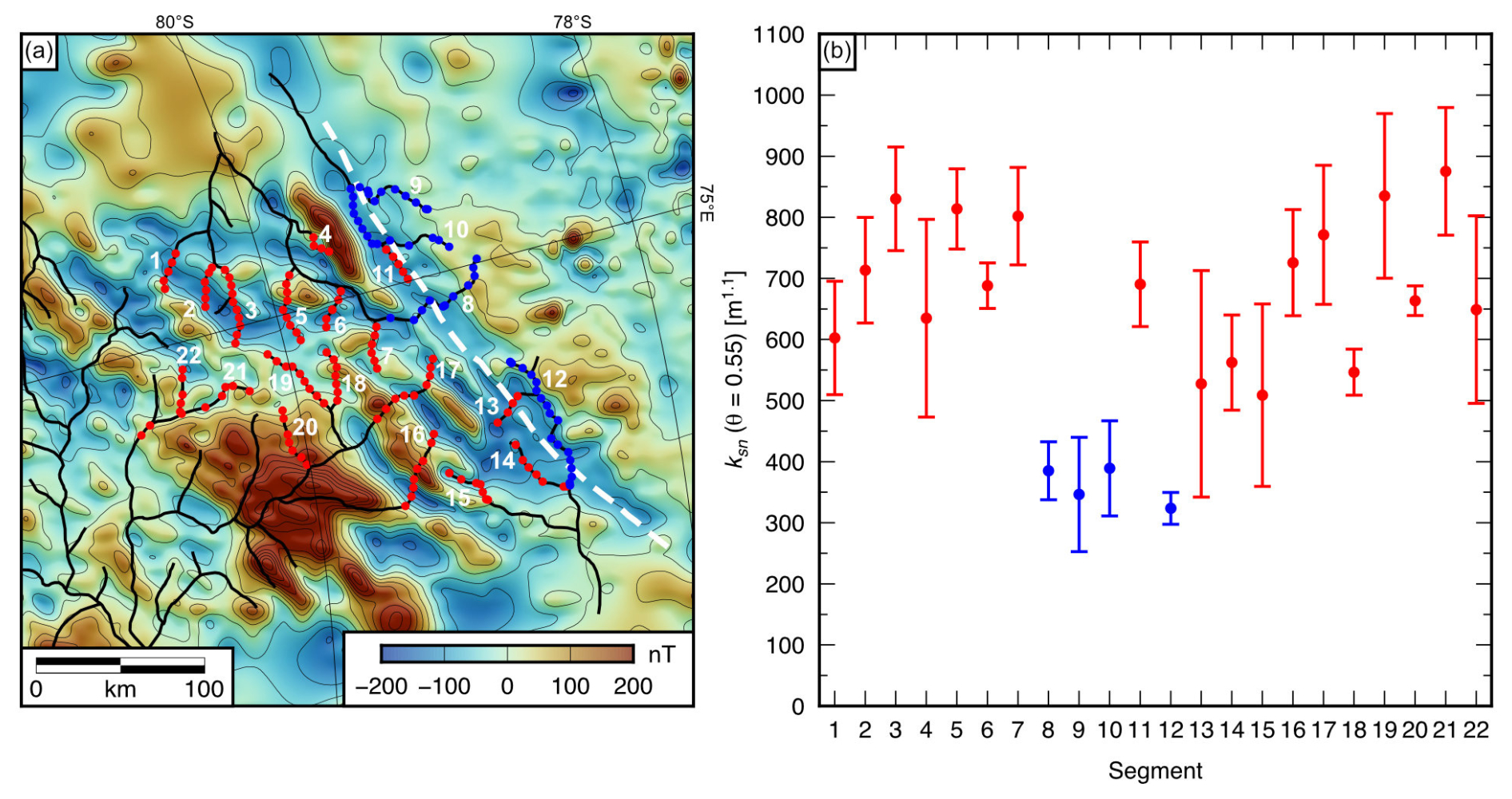
Figure 7 Normalised channel steepness indices in the northern GSM. (a) Valley network (black) with selected segments used for χ analysis (coloured circles and white numbers; see Fig. S5 for χ-elevation plots for individual segments) overlain on the ADMAP-2B magnetic anomaly (Eagles et al., 2024; Golynsky et al., 2018). Contour interval is 50 nT. The dashed white line marks a major magnetic boundary. Panel extent is shown in Fig. 5a. (b) Normalised channel steepness index (k_sn; corresponding to θ_ref = 0.55) for each of the 22 valley segments. Values of k_sn were computed from the gradient of the linear least-squares regression of the χ-elevation plot for each segment. Error bars denote ± 1 standard deviation. Blue and red colours denote valley segments differentiated by their k_sn values and position relative to the magnetic boundary.

In Sect. 4.1, we noted that longitudinal profiles in the northern GSM appear to have gentler slopes in the upper reaches than those in the central and southern GSM (Fig. 4). χ analysis allows us to normalise for the scaling of channel slope with drainage basin area across basins with different concavities and isolate geological/climatic controls on k_sn across the northern and central GSM. We divided the upper reaches of basins 4, 5, 6, 7, and 8 into 22 segments of approximately equal length (∼ 50 km; Fig. 7a) and computed k_sn from the χ-elevation plots where θ_ref = 0.55 (Fig. S5). We found a dichotomy of k_sn values across the northern GSM. Of the 22 segments, 18 were characterised by a k_sn of 350–950 m^1.1, while four were characterised by a value of 250–450 m^1.1 (Fig. 7b). The four segments with lower steepness indices were clustered in the northernmost GSM. The spatial boundary between the two groups of channel segments coincides with a transition in the intensity and pattern of the magnetic anomaly, with east–west-trending short-wavelength (10–20 km) anomalies with amplitudes of up to ± 200 nT to the south and a lower-amplitude signal lacking in lineations to the north (Fig. 7a).

4.3 Longitudinal profile evolution

Our first stream power incision modelling experiment for basin 10 assumed a constant U, m = 0.60, and n = 1 (Eq. 11). However, we note that χ analysis revealed that segments 2 and 3 had different k_s values (Fig. 6b), which (according to Eq. 6) reflects a difference in U and/or K. Given that the boundary between the segments is relatively abrupt, is observed across multiple tributaries within the network, and corresponds with a magnetic anomaly transition (Fig. 6c–e), we hypothesise that a lithological boundary with a step-change in K is most likely responsible for the different k_s values.

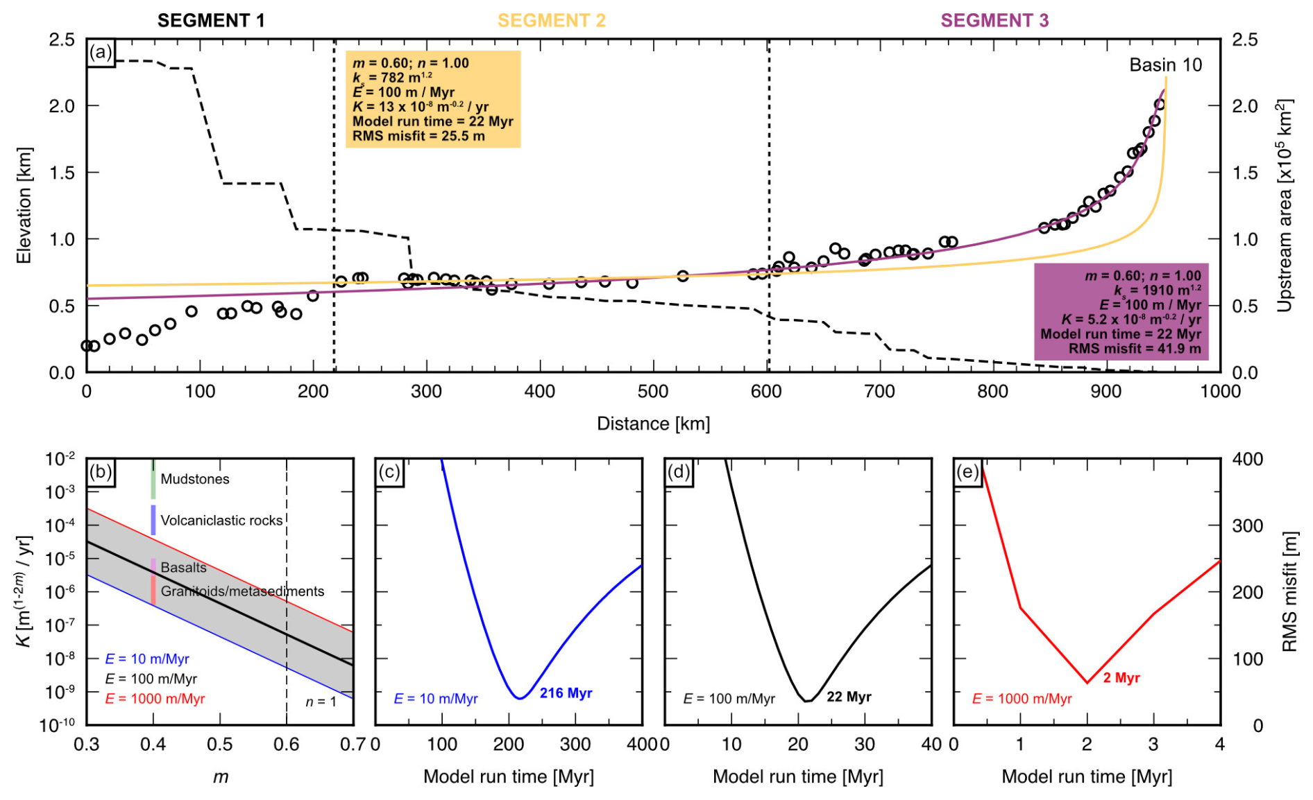
Figure 8 Stream power incision modelling with uniform uplift rate. (a) Comparison between modelled (coloured lines) and observed (circles) longitudinal profiles for GSM basin 10. The stepped dashed line marks the upstream drainage area as a function of distance along the profile. Vertical dashed lines mark boundaries between profile segments. The models shown used K values calculated assuming E = 100 m Myr⁻¹; different values of K are used for segments 2 and 3 depending on k_s. The best-fitting model profiles for E = 10 and 1000 m Myr⁻¹ are almost identical in shape but require ∼ 10× longer and ∼ 10× shorter model run times, respectively. (b) Covariance of K and m. The shaded region corresponds to an E range of 10–1000 m Myr⁻¹ (for the k_s value of segment 3). Coloured horizontal bars denote ranges of K for different lithologies (Stock and Montgomery, 1999) where m = 0.40. Dashed line marks m = 0.60, the best-fitting value for GSM basin 10. (c–e) RMS misfit between the observed and modelled longitudinal profiles across segments 2 and 3 (panel a) as a function of model run time (which was varied in 1 Myr increments) for the three K scenarios corresponding to: (c) E = 10 m Myr⁻¹, (d) E = 100 m Myr⁻¹, and (e) E = 1000 m Myr⁻¹. The best-fitting model run time (with the minimum RMS misfit) is indicated in each panel.

To test this hypothesis, we ran the SPIM for K values corresponding to the k_s values recovered from χ analysis for segments 2 and 3 (Fig. 6b). For these models we calculated K ranges using Eq. (12) for E = 10–1000 m Myr⁻¹ (Fig. 8a and b). The computed K values were 1.3–130 × 10⁻⁸ ${\mathrm{m}}^{-\mathrm{0.2}}{\mathrm{yr}}^{-\mathrm{1}}$ for segment 2 and 0.52–52 × 10⁻⁸ ${\mathrm{m}}^{-\mathrm{0.2}}{\mathrm{yr}}^{-\mathrm{1}}$ for segment 3. When adjusted for covariance with m, these K estimates (particularly for E = 10–100 m Myr⁻¹) are in close agreement with the range derived for granitoids and metasedimentary rocks (Stock and Montgomery, 1999), which have values substantially lower than other lithological groups such as basalt flows, volcaniclastics, and mudstones (Fig. 8b).

For a given value of E, the modelled longitudinal profile yields a close fit to observed elevations within segment 3 when a lower K value is used, and an improved fit with the more gradual slope of segment 2 when a higher K value is used (Fig. 8a). The model run times that yielded the best fit to the observed profile across both segments (by minimising the RMS misfit between the observed and modelled elevations) were: 216 Myr when E = 10 m Myr⁻¹, 22 Myr when E = 100 m Myr⁻¹, and 2 Myr when E = 1000 m Myr⁻¹ (Fig. 8c–e). The model with different K values for segments 2 and 3 has a combined RMS misfit of 36.7 m, which is lower than the misfits if either K value is used for the entire reach. This result confirms the findings of the χ analysis and indicates that the profile crosses a lithological boundary with a step-change in K at ∼ 600 profile-km.

However, these simulations cannot account for the presence of the two knickpoints within segment 1, which have higher slopes than the regional trend (Fig. 8a). These features may be: (i) static due to a spatial change in lithology (K) or uplift rate (U) or due to profile modification by past glacial erosion or (ii) reflect a transient response of the profile to base-level fall, whereby the knickpoints would have been propagating upstream. In our second modelling experiment, we used the SPIM and Eq. (13) to calculate the time taken for the two knickpoints to propagate to their observed positions, assuming they started at base level, which is taken to be the lowermost point on the profile (see Sect. 4.4). This experiment resulted in an improved fit with the observed elevations in segment 1 of the profile (Fig. S6). For a range of parameter space including E = 10–1000 m Myr⁻¹, $m/n$ = 0.5–0.6, and n = 0.8–1.2, the maximum response time required for the lower and upper knickpoints to propagate to their observed locations are ∼ 6.3 and ∼ 18 Myr, respectively. This suggests that if these knickpoints are indicative of base-level fall, they formed a relatively short amount of time before EAIS growth and the associated shut-down of fluvial incision. We discuss the origin and significance of the knickpoints further in Sect. 5.3.

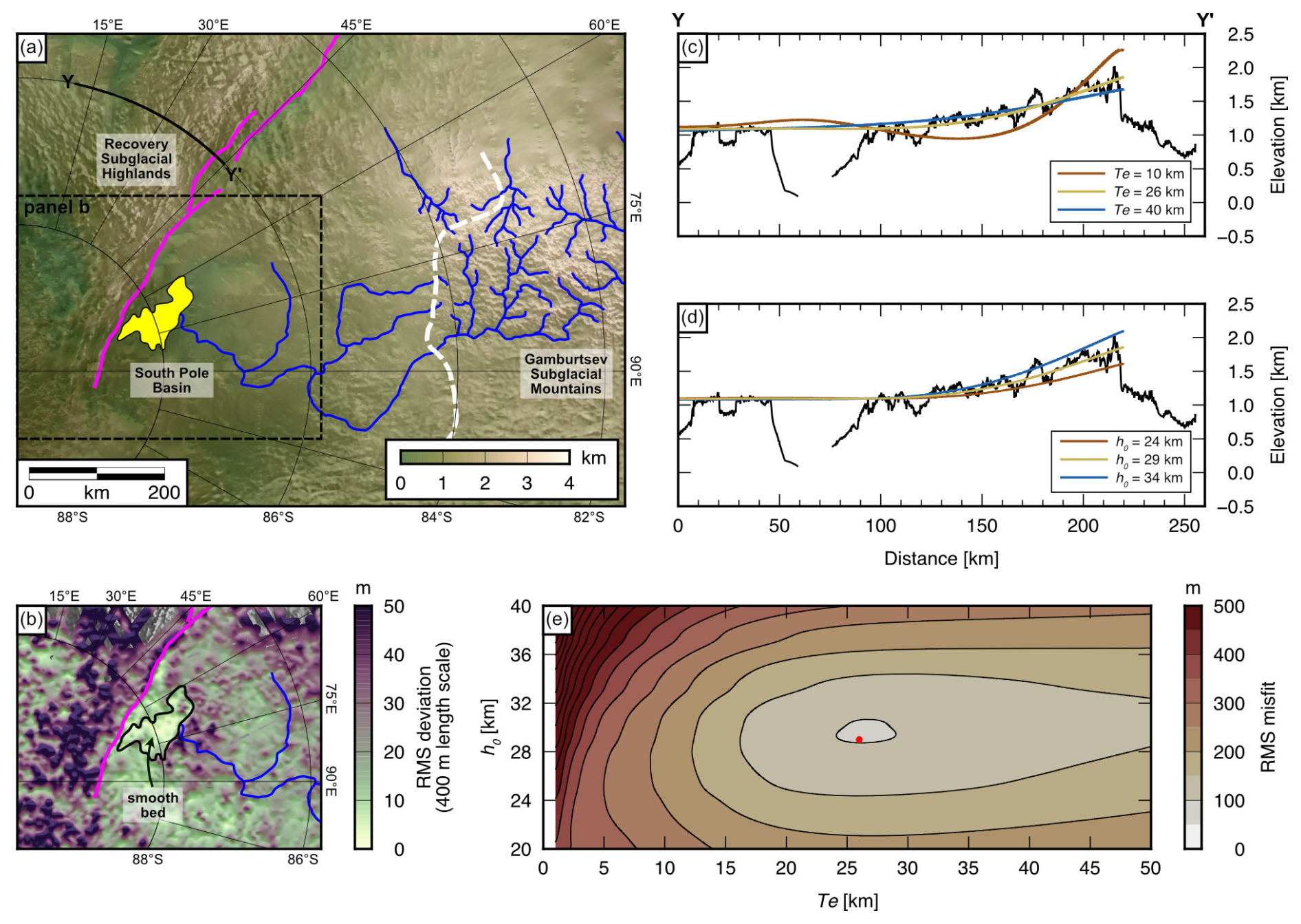
Figure 9 Base level for the southern GSM. (a) Relationship between the valley network (blue), South Pole Basin (SPB), and the Recovery Subglacial Highlands (RSH) fault system (purple). White dashed line marks the geological boundary inferred from longitudinal profile analysis and magnetic anomalies (Fig. 6). Dashed box marks the extent of panel (b). Bed elevations are derived from the rebounded Bedmap3 DEM (Paxman et al., 2022; Pritchard et al., 2025); shading is from the RADARSAT RAMP AMM-1 SAR image mosaic version 2 (Jezek et al., 2013). (b) RMS deviation of bed elevation over a 400 m length scale within the SPB and RSH (Young et al., 2025). The area marked by the black outline (filled yellow in panel a) has smooth bed (RMS deviations < 10 m). (c) Flexural modelling of bed topography along profile Y–Y^′. Black line is bed elevation isostatically adjusted for the removal of the present-day ice-sheet load (Paxman et al., 2022). Coloured lines show the flexural uplift profiles computed using a 1D elastic plate model. Flexure is caused by a combination of erosional unloading and mechanical unloading along a normal fault system (Fig. S8). Profiles are shown for three effective elastic thickness (Te) values, with a faulted layer thickness (h₀) of 29 km. (d) As for panel (c), except coloured profiles are shown for three h₀ values with a Te of 26 km. (e) RMS misfit between the observed and modelled topography across the RSH as a function of Te and h₀. Contour interval is 50 m. The red circle marks the best-fitting combination; Te = 26 km; h₀ = 29 km.

4.4 Base level and tectonic structure south of the Gamburtsevs

The region south of the Gamburtsevs, where the longitudinal profile of basin 10 appears to terminate, is characterised by a major north–south-trending topographic lineament visible in the RAMP AMM-1 SAR image mosaic (Fig. 9a). To the west of this lineament is the rugged and elevated topography of the RSH, which contrasts with the smoother, low-lying terrain of the SPB east of the lineament (Fig. 9b). The valley network of basin 10 can be traced to a part of SPB characterised by conspicuously low RMS deviations of bed elevation (< 10 m; Fig. 9b), which are indicative of low roughness over length-scales of > 100 m (Young et al., 2025). Moreover, RES imaging reveals a bed with high specularity content in this area (> 0.4; Fig. S7), which is indicative of low roughness at small (i.e., decimetre) scales (Schroeder et al., 2015; Young et al., 2025). This smooth region, measuring approximately 100 km × 50 km, is contained within an enclosed topographic basin (Fig. S7) and therefore likely constituted base level for basin 10 prior to EAIS formation.

RES imaging shows that the RSH exhibit an asymmetric cross-sectional profile, with a steep escarpment at their eastern margin that is expressed as the lineament visible in the RAMP AMM-1 SAR image mosaic (Fig. 9a). The highlands are tilted westwards away from the escarpment at an angle of ∼ 0.3° (Fig. 9c and d). Flexural modelling indicates that this topography is consistent with uplift and tilting of the highlands due to a combination of: (i) mechanical unloading on an extensional fault system located at the base of the escarpment and (ii) erosional unloading of material excavated from the large troughs on either side of the highlands (Fig. S8). By computing the theoretical pattern of flexure and comparing to the observed escarpment relief and highland tilt, we recovered a best-fitting effective elastic thickness (Te) of 26 km and a faulted layer thickness of 29 km (Figs. 9c–e and S8).

A swath of topographic profiles along-strike of the RSH shows that ice-free elevations increase from ∼ 1000–1200 m at the southern end of the range to ∼ 1500–1700 m to the north (Fig. S9). This change in elevation occurs over a length scale of ∼ 25 km and coincides with an increase in RSH half-width to ∼ 15 km (Fig. S9). The position of this step-change in RSH elevation and half-width coincides with the southern edge of the escarpment and the location of the smooth basin on the hanging-wall side of the range front (Fig. S9).

5 Discussion

5.1 Fluvial landscape preservation and glacial modification

There are multiple lines of evidence from the valley longitudinal profiles indicating that elements of the pre-glacial fluvial landscape are preserved in the Gamburtsevs. First, the trunk valleys and tributaries are concave-up and the recovered concavity indices are consistent with fluvial systems. The m and n exponents covary (Croissant and Braun, 2014), meaning their ratio theoretically and empirically falls within a relatively narrow range of 0.3–0.7 (Smith et al., 2022); all our recovered θ values (0.50–0.61) lie within this range. Second, when plotted in χ-elevation space, the longitudinal profiles are transformed to a single straight line (or two linear segments associated with different k_sn values in the case of basin 10). This behaviour is diagnostic of steady-state fluvial landscapes (Perron and Royden, 2013). Exceptions include the upper reaches of basin 8 (Fig. 5d and e) and the lower reaches of basin 10 (Fig. 6b), which are discussed below. Third, the trunk valley and tributaries show strong collinearity in χ-elevation space (Fig. S4), as would be expected for steady-state fluvial systems (Mudd et al., 2018). These findings are supported by the ability of the SPIM to replicate the observed longitudinal profiles for a simple set-up where only the values of m, n, and K are varied between basins (Fig. 8).

However, we note that some features of the longitudinal profiles are inconsistent with fluvial incision, and instead likely reflect glacial modification of the fluvial landscape at, or prior to, ca. 34 Ma. For example, several profiles show localised deviations below the “expected” fluvial profile generated via the SPIM, particularly in the central and northern GSM (Fig. 5). These overdeepenings are up to ∼ 300 m deep and often coincide with tributary junctions (Fig. 5). These observations are consistent with expectations for glacial overdeepenings, formed by enhanced erosion at points where warm-based valley glaciers (that likely exploited inherited fluvial valleys) converge, causing ice flow to accelerate (Cook and Swift, 2012; Lloyd et al., 2023). Incision by subglacial meltwater may have also contributed, but the coincidence of overdeepenings with tributary junctions is strongly indicative of valley glacier erosion. Moreover, the amplitude of the profile undulations exceeds that typically observed in channels incised into bedrock by subglacial meltwater and the valleys do not display the U-shaped, anastomosing forms typically associated with large subglacial flood events (Kehew et al., 2012; van der Vegt et al., 2012).

We also note that the upper part of basin 8 deviates significantly from the modelled fluvial profile and the straight line in the χ-elevation plot (Fig. 5d and e). The basin exhibits steepened “headwaters” and a gentle slope immediately below, before reaching an inflection point at ∼ 190 profile-km where the observed profile “rejoins” the SPIM profile and the slope increases. These observations are consistent with the expected morphology of fluvial profiles whose upper reaches have been modified by valley glaciation (Anderson et al., 2006; Deal and Prasicek, 2021). We also infer that the elevation of the inflection point (∼ 1500 $\mathrm{m}\mathrm{a}.\mathrm{s}.\mathrm{l}.$) gives an approximate indication of the palaeo-equilibrium line altitude/ice limit, which would have been associated with efficient glacial erosion (Brocklehurst and Whipple, 2006).

These findings confirm that the fluvial landscape of the Gamburtsevs was erosively modified by mountain-scale glaciation, most likely during, or prior to, EAIS growth at ca. 34 Ma (Rose et al., 2013). We also find that glacial modification appears to have been greater in the central and northern Gamburtsevs, which are characterised by higher elevations than the southern Gamburtsevs (Fig. 3b) and are closer to the coast, so may have been associated with higher precipitation rates. Profile overdeepening of up to ∼ 300 m by warm-based valley glaciers would have required multiple glacial-interglacial cycles to achieve, assuming typical erosion rates (Koppes and Montgomery, 2009). However, in all basins, particularly at lower elevations and in the southern GSM (basin 10), elements of the steady-state fluvial topography are well preserved. This suggests that the coalescence of a continental-scale EAIS occurred rapidly and/or non-erosively at, or shortly after, ca. 34 Ma (Jamieson et al., 2010; Van Breedam et al., 2022), and that since then the GSM landscape has been preserved beneath slow-moving ice. Indeed, contemporary ice-surface velocities are < 5 m yr⁻¹ and ice is frozen to the bed, with implied negligible erosion rates (Creyts et al., 2014; Mouginot et al., 2019; Seiner et al., 2025). This supports the hypothesis that, although the EAIS has experienced some retreat during past warm climate intervals (Aitken et al., 2016; Halberstadt et al., 2024; Sangiorgi et al., 2018), a cold-based, slow-moving core has continuously persisted over the GSM (Jamieson et al., 2010). This has likely been aided by the high elevation and roughness of the mountains, which “pin” the overlying ice sheet and inhibit fast flow owing to high basal friction (Bingham and Siegert, 2009).

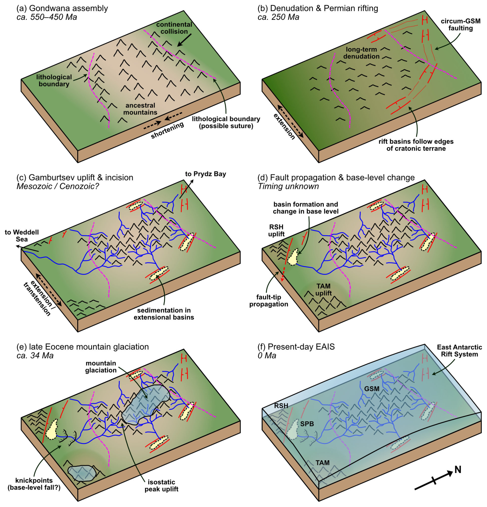
Figure 10 Schematic long-term landscape evolution scenario for the Gamburtsev region. (a) Continental collision in the Cambro-Ordovician resulted in Gondwana assembly and the formation of major geological boundaries/sutures. (b) Long-term denudation reduced the relief of interior East Antarctica. Permian extensional deformation resulted in the formation of the East Antarctic Rift System, which likely exploited more mobile belts around cratonic terranes. (c) Uplift of the contemporary Gamburtsevs most likely commenced in the Mesozoic or early Cenozoic. River networks incised the mountains and deposited sediments in the interior rift basins as well as routing material to Prydz Bay to the north and the Weddell Sea to the south. (d) The fault system bounding the RSH propagated towards the South Pole, cutting off the drainage pathway to the Weddell Sea and forming an interior depocentre in the SPB. (e) Base-level fall prior to glaciation formed two knickpoints upstream of the SPB. Mountain glaciation commenced on the high terrain of the GSM and Transantarctic Mountains (TAM) in the Eocene. (f) The EAIS rapidly expanded at ca. 34 Ma and preserved the subglacial landscape due to negligible erosion rates.

5.2 Lithological and tectonic structure of the Gamburtsevs and surrounding regions

In this section, supported by Fig. 10, we discuss the geological structure and evolution of the GSM and the East Antarctic interior. The distribution of k_sn values recovered from the longitudinal profiles, combined with spatial patterns in the magnetic anomaly and its derivatives (Figs. 6 and 7), indicate that the southern and northern margins of the GSM are bounded by major geological structures. In the northern GSM there is a transition in the intensity and pattern of the magnetic anomalies across a linear divide (Fig. 7a). The position of this boundary coincides with a step-change in k_sn values, which are approximately twice as high for channels on the southern side of the boundary than the northern side (Fig. 7b). The observed magnetic dichotomy has previously been inferred to mark the position of a suture between geological terranes, likely originating from the assembly of Gondwana at ca. 500 Ma (Ferraccioli et al., 2011) (Fig. 10). The suture is hypothesised to demarcate an accretionary fold-and-thrust terrane to the south and an arc terrane to the north (Wu et al., 2023). Although differences in k_sn can also be attributable to changes in uplift rate (Eq. 6) and K is also dependent on non-geological factors such as sediment flux characteristics and hydraulic geometry (Whipple and Tucker, 1999), the coincidence of this abrupt k_sn change with the magnetic anomaly transition supports the presence of a step-change in lithology (and thus K) across this boundary. As well as being consistent with hypotheses from crustal modelling (Ferraccioli et al., 2011; Wu et al., 2023), our results imply lower bedrock erodibilities in the central GSM than to the north of the suture.

At the southern edge of the GSM, the valleys in basin 10 cross a boundary where k_sn decreases (moving southwards) by a factor of ∼ 2.6 (Fig. 6b). This step-change is observed in multiple tributaries and coincides with a change in the frequency content of the magnetic anomaly (Fig. 6c–e), meaning we infer that it also reflects a major lithological boundary. This contact appears to approximately align with the mooted boundary between the GSM and the weakly-magnetic South Pole Province, whose geology is poorly understood (Ferraccioli et al., 2011; Wu et al., 2023). Our findings indicate that the South Pole Province is characterised by higher bedrock erodibilities than the GSM. Although our results alone cannot be used to assign a specific lithology to the GSM or the regions to the north and south, we note that our K estimates (when adjusted for m) are at the lower end of reported values (Stock and Montgomery, 1999), corresponding to those of erosion-resistant lithologies such as granitoids and metasedimentary rocks (Fig. 8b). Indeed, the exposed margins of East Antarctica are dominated by resistant rock-types, including Archaean–Neoproterozoic gneisses and Neoproterozoic–Palaeozoic metasediments (Cox et al., 2023). The magnetic signatures observed in the GSM, including high-amplitude anomalies with a distinct structural “grain” (e.g., Fig. 7a), have been used to inform hypotheses that the Gamburtsevs may comprise an early Palaeozoic accretionary orogenic belt associated with magmatic intrusions, superimposed on Archaean–Proterozoic basement orthogneiss (Ferraccioli et al., 2011; Wu et al., 2023). Although our findings do not offer any further direct constraints on GSM lithology, we note that: (i) these proposed low-erodibility terranes are consistent with observed channel steepness indices, and (ii) structures within the orogenic belt may have continued to influence drainage patterns until ice-sheet nucleation.

South of the GSM, we propose that the RSH represent an uplifted highland block in the footwall of an extensional fault system. There are three lines of evidence to support this hypothesis. First, the eastern side of the RSH is bounded by a linear escarpment (Figs. 9 and S7). Second, the topography of the RSH block is tilted away from the escarpment, as is expected for the pattern of flexural uplift due to mechanical unloading of the lithosphere in the vicinity of a normal fault (Fig. S8) (Ebinger et al., 1991; Weissel and Karner, 1989). Third, the drop-off in block width and relief at the southern end of the RSH (Fig. S9) is consistent with expectations of the topography at the propagating tip of a normal fault system (Densmore et al., 2005, 2007). This evidence for southward fault tip propagation, combined with observed low-magnitude extensional earthquake events (Lough et al., 2018), implies that this fault system may have accommodated extensional deformation and triggered uplift at the southern end of the RSH as recently as the Cenozoic (before and/or after Oligocene glaciation). We hypothesise that this fault propagation may have cut off a palaeo-fluvial drainage pathway between the GSM and the Weddell Sea via the Pensacola-Pole Basin (Fig. 1b), which would have implications for sediment provenance (Licht and Hemming, 2017) and regional base level for the Gamburtsevs (Fig. 10).

Deeper crustal and lithosphere structure also has important implications for ice-sheet dynamics. The best-fitting Te for the RSH of 26 km (Fig. 9c) is comparable to values recovered from the East African Rift (Daly et al., 2020; Ebinger et al., 1991). Moreover, the best-fitting faulted layer thickness of 29 km (Fig. 9d) is in good agreement with estimates from East Africa, which is associated with a thicker brittle layer (25–30 km) than many rifts due to inherited thick cratonic lithosphere and/or low heat flow (Lavier and Buck, 2002). Earthquake events in this part of East Antarctica are located at depths of up to 30 km beneath the ice surface (Lough et al., 2018), supporting the presence of a thick brittle layer. This suggests that this part of the East Antarctic interior is associated with thick lithosphere and low heat flow, as is inferred from seismic tomographic analysis (Hazzard et al., 2023).

To the east of the RSH, the hanging-wall topography of the South Pole Basin is lower-lying and less rugged (Fig. 9). Within the SPB is a particularly smooth and flat-lying enclosed region (Fig. 9b) with an area of ∼ 4800 km². This is comparable to the Great Salt Lake (Utah, USA), which is similarly situated in the hanging-wall of a major range-bounding normal fault system in a continental interior. Given these observations and the fact that the basin 10 valley network originating in the southern GSM appears to terminate at this location (Fig. 9), we propose that this smooth basin: (i) formed due to subsidence of the hanging-wall of the RSH fault system, (ii) would likely have been endorheic and constituted the local base level for the southern GSM if it existed prior to glaciation, and (iii) may contain sedimentary material transported from the Gamburtsevs by river systems prior to ca. 34 Ma. We acknowledge the possibility that further sediment deposition within the basin has occurred subglacially (Young et al., 2025) but, given the lack of evidence for any major change in regional palaeotopographic configuration since glaciation (Paxman, 2023), this would have been a natural area for pre-glacial sediment accumulation in the East Antarctic interior (Fig. 10). We propose that this smooth region, situated beneath ∼ 3.5 km of ice, could be a promising future target for sub-ice drilling programmes with the ambition of recovering detrital sedimentary material sourced from the southern GSM. Analysis of such material would potentially provide important constraints on East Antarctic uplift and erosion histories, lithology and sediment provenance, palaeoclimate, and the nature of early glaciation.

5.3 Timing of Gamburtsev uplift

In this section we explore the extent to which stream power incision modelling enables constraints to be placed on the age of the fluvial landscape, which would in turn constrain the timing of Gamburtsev uplift. We emphasise that the SPIM is underconstrained, primarily due to the ambiguity regarding long-term erosion rates in interior East Antarctica, making a precise reconstruction of uplift history impossible without further constraints. We instead ask whether, for a plausible parameter space, we can place realistic bounds on uplift history and compare this to existing hypotheses for GSM evolution. In this context, the most important constraint to establish is the upper (i.e., oldest) age limit of onset of GSM uplift and fluvial incision.

For the low end-member erosion-rate scenario used in our longitudinal profile modelling (E = 10 m Myr⁻¹), we found a best-fitting model run time of 216 Myr for basin 10 (Fig. 8c). Increasing E to 100 and 1000 m Myr⁻¹ reduced the model run time to 22 and 2 Myr, respectively. Despite the difference in erosion rate, these latter two scenarios both imply that uplift occurred in the early Cenozoic. If fluvial erosion was “switched off” following EAIS growth at ca. 34 Ma, the implied age range for the commencement of GSM uplift is ca. 250–36 Ma. Thermochronological evidence from the Transantarctic Mountains and the Lambert Glacier-Prydz Bay region, using detrital material that may have been eroded from the continental interior of East Antarctica including the GSM, records four regional tectonic/magmatic/exhumation events in the Phanerozoic (Fitzgerald and Goodge, 2022; Thomson et al., 2013) that represent candidate intervals for GSM uplift:

• 1.

  Cambro-Ordovician (ca. 500 Ma) metamorphism, magmatism and subsequent cooling occurred in relation to collisional orogeny during Gondwana assembly (Fitzgerald and Goodge, 2022; Thomson et al., 2013).

• 2.

  Permo–Triassic (ca. 300–250 Ma) cooling and exhumation was likely caused by intra-continental rifting, which has been hypothesised to have been a trigger for GSM uplift (Ferraccioli et al., 2011; Thomson et al., 2013).

• 3.

  Early Jurassic (ca. 180 Ma) cooling is observed in some samples from the Transantarctic Mountains and indicative of exhumation accompanying extension relating to Gondwana breakup (Fitzgerald and Goodge, 2022).

• 4.

  Cooling and exhumation in the mid-Cretaceous (ca. 125–90 Ma) may have been related to reactivation of the East Antarctic Rift System to accommodate interior transtensional deformation (Ferraccioli et al., 2011; Fitzgerald and Goodge, 2022; Phillips and Läufer, 2009; Thomson et al., 2013).

Our results preclude any model in which GSM uplift occurred solely during Gondwana assembly. Collisional uplift of an “ancestral” Gamburtsev mountain range in the early Palaeozoic is possible (Fitzgerald and Goodge, 2022) – the geological boundaries recorded by the channel steepness indices (Figs. 6 and 7) may reflect this amalgamation (Ferraccioli et al., 2011; Wu et al., 2023) – but subsequent denudation followed by later, renewed uplift would be necessary. Permo–Triassic rifting is at the uppermost limit of our feasible age range, meaning it would necessitate markedly low erosion rates (∼ 10 m Myr⁻¹) after ca. 250 Ma to have been the primary cause of GSM uplift. As discussed in Sect. 3.3, erosion rates of this magnitude would be anomalously low for a steep, high-relief mountainous area, and we conclude that it is probable that the uplift and incision of the fluvial landscape preserved in the GSM occurred more recently than ca. 250 Ma.

We therefore propose that the fluvial incision preserved in the landscape of the GSM most likely occurred in response to uplift that commenced in the late Mesozoic or early Cenozoic (Fig. 10). This would correspond to more plausible erosion rates of ∼ 50–100 m Myr⁻¹ (or higher; see Sect. 3.3). The trigger for this uplift may have been mid-Cretaceous deformation (event (4) above), Eocene geodynamic uplift causally related to earlier Gondwana breakup (Gernon et al., 2026), or an alternative, previously unrecognised, mechanism. In the case of mid-Cretaceous reactivation of the East Antarctic Rift System, we may expect topographic structures indicative of transtensional deformation to be preserved in the regions surrounding the GSM, which are poorly surveyed by radio-echo sounding. We suggest that future mapping and analysis of topographic lineaments and/or the planform patterns of subglacial valley networks and drainage basins (Mudd et al., 2022) using improved techniques for mapping the texture of the bed topography (Ockenden et al., 2026) may enable this hypothesis to be tested in the future.

Finally, we note that the presence of knickpoints in the lower reaches of basin 10 means a proportion of the uplift may have occurred a relatively short amount of time before glaciation at ca. 34 Ma. We believe it is unlikely that these features formed due to glacial modification of the valley profile because they are situated > 700 km downstream of the profile “headwaters” and well beyond the reconstructed limit of late Eocene mountain-scale glaciation (Figs. 5a and 6c) (Rose et al., 2013), and because the observed profile upstream of the knickpoints is well fit by the SPIM profile (Fig. 8a). There are three other scenarios that may explain the presence of these knickpoints (Lague, 2014): (i) static knickpoints due to a change in lithology (spatial variation in K), (ii) static knickpoints due to the presence of faults (spatial variation in U), or (iii) upstream-propagating knickpoints due to base-level fall (temporal variation in U).

Although there is no obvious magnetic anomaly transition associated with the knickpoints, there is insufficient evidence to rule out any of these scenarios definitively. Hypothetically, for the scenario where the knickpoints are transient features arising from uplift/base-level fall and concomitant incision, their combined “relief” constrains the amount of base-level fall (over two phases) to ∼ 470 m. Based on Eq. (13), the upper limit for the time for the upper knickpoint to propagate upstream to its observed position (assuming the mapped profile starts at base level) is 18 Myr. If fluvial incision were “switched off” at ca. 34 Ma, this implies that the base level fall occurred between 52 and 34 Ma. Base-level fall may have been caused by subsidence in the vicinity of the SPB (e.g., due to extensional fault activity; see Sect. 5.2) and/or uplift of the GSM (Fig. 10). If such an event did occur, its timing may have had important implications for the nature and timing of Antarctic glacial inception. For a standard environmental lapse rate of ∼ 6.5 °C km⁻¹, uplift of ∼ 470 m would decrease surface temperatures over the tops of the mountains by ∼ 3–4 °C, potentially facilitating the onset of alpine glaciation and triggering the series of ice-sheet-climate feedbacks that paved the way for EAIS growth at ca. 34 Ma (DeConto and Pollard, 2003) (Fig. 10).

6 Conclusions

In this study, we have analysed valley longitudinal profiles from the Gamburtsev Subglacial Mountains, East Antarctica. Our aim was to shed light on the geological structure of the mountains, the tectonic and surface processes that have shaped the regional topography, and the timing of valley incision. Based on our findings, we conclude the following:

• 1.

  Gamburtsev valley longitudinal profiles retain features consistent with a steady-state fluvial landscape that formed prior to glaciation and has been preserved since EAIS growth at ca. 34 Ma. Minor localised modification of the landscape by mountain ice fields and glaciers occurred during the early stages of East Antarctic glaciation (at or prior to ca. 34 Ma), primarily in the central and northern Gamburtsevs.

• 2.

  Channel steepness indices and magnetic anomalies suggest that major geological boundaries are present at the northern and southern edges of the Gamburtsevs, with the lowest bedrock erodibilities found within the core of the mountain range. This demonstrates the potential for preserved valley longitudinal profiles to record variations in subglacial geology.

• 3.

  Stream power incision modelling suggests that uplift of the Gamburtsevs and incision of the fluvial landscape commenced no earlier than the early Mesozoic (ca. 250 Ma) and was likely much younger. We suggest that a substantial component of GSM uplift likely occurred in the late Mesozoic and/or early Cenozoic.

• 4.

  Material eroded from the southern Gamburtsevs was transported towards a base level near the South Pole, where sediments derived from the mountains may be preserved in interior depocentres formed due to extensional faulting. The South Pole Basin may be a promising target for recovery of detrital sedimentary material sourced from the southern GSM via future sub-ice drilling.