Groundwater erosion of coastal gullies along the Canterbury coast (New Zealand): a rapid and episodic process controlled by rainfall intensity and substrate variability

Gully formation has been associated to groundwater seepage in unconsolidated sand- to gravel-sized sediments. Our understanding of gully evolution by groundwater seepage mostly relies on experiments and numerical simulations, and these rarely take into consideration contrasts in lithology and permeability. In addition, process-based observations and detailed instrumental analyses are rare. As a result, we have a poor understanding of the temporal scale of gully formation by groundwater seepage and the influence of geological heterogeneity on their formation. This is particularly the case for coastal gullies, where the role of groundwater in their formation and evolution has rarely been assessed. We address these knowledge gaps along the Canterbury coast of the South Island (New Zealand) by integrating field observations, luminescence dating, multi-temporal unoccupied aerial vehicle and satellite data, time domain electromagnetic data and slope stability modelling. We show that gully formation is a key process shaping the sandy gravel cliffs of the Canterbury coastline. It is an episodic process associated to groundwater flow that occurs once every 227 d on average, when rainfall intensities exceed 40 mm d⁻¹. The majority of the gullies in a study area southeast (SE) of Ashburton have undergone erosion, predominantly by elongation, during the last 11 years, with the most recent episode occurring 3 years ago. Gullies longer than 200 m are relict features formed by higher groundwater flow and surface erosion > 2 ka ago. Gullies can form at rates of up to 30 m d⁻¹ via two processes, namely the formation of alcoves and tunnels by groundwater seepage, followed by retrogressive slope failure due to undermining and a decrease in shear strength driven by excess pore pressure development. The location of gullies is determined by the occurrence of hydraulically conductive zones, such as relict braided river channels and possibly tunnels, and of sand lenses exposed across sandy gravel cliffs. We also show that the gully planform shape is generally geometrically similar at consecutive stages of evolution. These outcomes will facilitate the reconstruction and prediction of a prevalent erosive process and overlooked geohazard along the Canterbury coastline.

1 Introduction

1.1 Coastal gullies

Gullies can be incised into coastal cliffs and bluffs in a variety of geologic settings around the world, owing their formation to a complex interaction of hydrologic, lithospheric, tectonic and atmospheric processes. While much research has focused on gully formation and evolution in non-coastal settings in response to changes, such as land cover and use, natural hazards and/or changes in precipitation, relatively little work has focused on gully geomorphology and morphodynamics in coastal cliffs and bluffs. The most commonly accepted mechanism for coastal gully formation is through concentrated overland flow and knick point migration (Ye et al., 2013; Leyland and Darby, 2008, 2009; Mackey et al., 2014; Limber and Barnard, 2018). Changes in land cover and use due to agriculture, logging, forest fires and other factors can decrease surface roughness and increase concentrated overland flow, which, given sufficient energy and/or time, can erode a narrow section of coastal cliff and form a knick point. Depending on the resistive forces (e.g. geology and uplift) relative to the erosive force of the overland flow, this knick point will migrate inland over time, incising a gully into the cliff or bluff. Recent work has focused on modelling coastal gully formation and evolution as knick point migration (Limber and Barnard, 2018).

Coastal cliff stability and gully incision can be affected by processes of concentrated overland flow, quarrying by waves at the base of the cliff and groundwater discharge (Limber and Barnard, 2018; Kline et al., 2014), although it is unclear when and where each of these factors is important (Collins and Sitar, 2009, 2011). While overland flow is a common formation mechanism, it is possible to have coastal gullies form where the cliff is affronted by a beach, which limits the basal quarrying or notching by waves, and where there is no outward sign of overland flow. Relatively little attention has been paid to the potentially important role of groundwater as a driver of coastal gully formation and evolution, despite the potential for groundwater to affect the geotechnical properties of coastal cliffs (Collins and Sitar, 2009, 2011).

1.2 Channel erosion by groundwater seepage

Groundwater has been implicated as an important geomorphic agent in channel network development, both on Earth and on Mars (Kochel and Piper, 1986; Higgins, 1984; Dunne, 1990; Malin and Carr, 1999; Harrison and Grimm, 2005; Salese et al., 2019; Abotalib et al., 2016). The classic model entails a channel headwall that lowers the local hydraulic head and focuses groundwater flow to a seepage face. This leads to upstream erosion by undercutting, the rate of which is limited by the capacity of seepage water to transport sediment from the seepage face (Dunne, 1990; Howard and McLane, 1988; Abrams et al., 2009). Groundwater seepage has been shown to unambiguously lead to channel formation in unconsolidated sand- to gravel-sized sediments (Lapotre and Lamb, 2018; Dunne, 1990), e.g. gravel-braided river deposits in Alaska (Sunderlin et al., 2014) and the Canterbury Plains (Schumm and Phillips, 1986), conglomerates in the Kalahari (Nash et al., 1994), outwash and alluvial sands in Florida (Schumm et al., 1995), Martha's Vineyard (Uchupi and Oldale, 1994) and Vocorocas (Coelho Netto et al., 1988), dune sand and tephra in South Taranaki (Pillans, 1985), and granodiorite regolith in the Obara area of Japan (Onda, 1994). In sediments finer than sands, erosion is typically limited by detachment of the grains at the seepage face. In silts and clays, the permeability is so low that the groundwater discharge is often less than that required to overcome the cohesive forces of the grains (Dunne, 1990). The role of groundwater seepage and channel formation in bedrock, on the other hand, remains controversial (Lamb et al., 2006; Pelletier and Baker, 2011).

Our understanding of channel evolution by groundwater seepage is predominantly derived from theoretical, experimental and numerical models (Howard, 1995; Lobkovsky et al., 2004; Chu-Agor et al., 2008; Wilson et al., 2007; Petroff et al., 2011; Pelletier and Baker, 2011; Higgins, 1982). Such studies suggest that the velocity at which channel heads advance is a function of the groundwater flux and the capacity of seepage water to transport sediment from the seepage face (Fox et al., 2006; Howard and McLane, 1988; Abrams et al., 2009; Howard, 1988), and that channel head erosion occurs by episodic headwall slumping (Kochel et al., 1985; Howard, 1990). Channels incised by groundwater seepage have been shown to branch at a characteristic angle of 72^∘ at stream tips, which increases to 120^∘ near stream junctions (Devauchelle et al., 2012; Yi et al., 2017), whereas growing indentations competing for draining groundwater results in periodically spaced channels (Dunne, 1990; Schorghofer et al., 2004). Channel network geometry appears to be determined by the external groundwater flow field rather than flow within the channels themselves (Devauchelle et al., 2012).

A number of fundamental questions related to the evolution of channels by groundwater seepage in unconsolidated sediments remain unanswered. First, the temporal scale at which channels form is poorly quantified due to the paucity of process-based observations and detailed instrumental analysis. Field observations of groundwater processes are rare (e.g. Onda, 1994), primarily due to the difficulty with accessing the headwalls of active channels, the potentially long timescales involved and the complexity of the erosive process (Dunne, 1990; Chu-Agor et al., 2008). Quantitative assessments of channel evolution have relied on experimental and numerical analyses, but these tend to be based on simplistic assumptions about flow processes and hydraulic characteristics. Experimental approaches are based on a range of different methods, limiting comparison of their outcomes (Nash, 1996). Published erosion rates vary between 2–5 cm per century (Schumm et al., 1995; Abrams et al., 2009) and 450–1600 m³ per year (Coelho Netto et al., 1988). Second, the influence of geologic heterogeneities on channel evolution is also poorly understood. Lithological strength and permeability contrasts are rarely simulated by experimental and numerical analyses. Third, there are only a few places where the mechanisms by which seepage erosion occurs have been clearly defined (e.g. Abrams et al., 2009). Basic observations and measurements of channel erosion rates and substrate geologic heterogeneities are needed to test and quantify models for channel formation and improve our ability to reconstruct and predict landscape evolution by groundwater-related processes.

1.3 Objectives

In this study, we revisited the Canterbury Plains study site (Schumm and Phillips, 1986) and carried out field observations, geochronological analyses, repeated remote sensing surveys, near-surface geophysical surveying and slope stability modelling of coastal gullies to (i) identify the processes by which groundwater erodes gullies along the coast, (ii) assess the influence of geological/permeability heterogeneity on the gully formation process and (iii) quantify the timing of gully erosion and its key controls.

2 Regional setting

The flat to gently inclined Canterbury Plains, located in the eastern South Island of New Zealand, extend from sea level up to 400 m above sea level and cover an area of 185 km by 75 km (Fig. 1a). A series of high-energy braided rivers emerge from the > 3500 m high Southern Alps and flow southeastwards to the shoreline (Kirk, 1991). The plains were formed by the coalescence of several alluvial fans sourced from the these rivers (Leckie, 2003; Browne and Naish, 2003). The Quaternary sedimentary sequence comprises a > 600 m thick succession of cyclically stacked fluvio-deltaic gravel, sand and mud with associated aeolian deposits and palaeosols (Browne and Naish, 2003; Bal, 1996). The gravels consist of greywacke and represent a variety of channel-fill beds and bar forms, whereas the isolated bodies of sand are relict bars and abandoned channels. The interglacial sediments are better sorted and have higher permeability than the glacial outwash, resulting in a wide range of hydraulic conductivities (Scott, 1980). New Zealand's largest groundwater resource is hosted in the gravels down to at least 150 m depth (Davey, 2006). The upper Quaternary sediments are exposed along a 70 km long coastline southwest of the Banks Peninsula (Moreton et al., 2002). This coastline is retrograding at approximately 0.5–1 m yr⁻¹ and consists of cliffs fringed by mixed gravel and sand beaches (Gibb, 1978). The study area is a 2.5 km long stretch of cultivated coastline located 16 km to the southeast of Ashburton (Fig. 1b). The coastline within the study area consists of a 15–20 m thick exposure of poorly sorted and uncemented matrix-supported outwash gravel, which is capped by up to 1 m of post-glacial loess and modern soil (Berger et al., 1996). The cliff face is punctuated by ∼0.5 m thick lenses of sand or clean gravel.

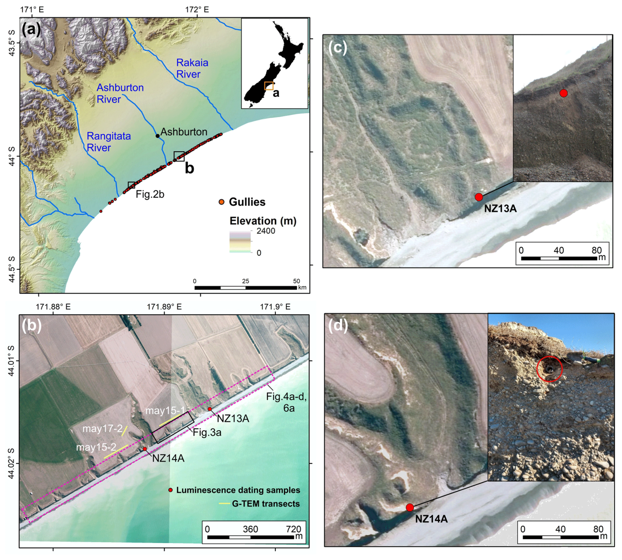
Figure 1 (a) Digital elevation model of the Canterbury Plains (source – Environment Canterbury), located along the eastern coast of the South Island of New Zealand, showing the location of mapped gullies. The location of figure is shown in the inset. (b) Mosaic of aerial photographs of the study area (see a for location; source – Environment Canterbury). The location of luminescence dating (optically stimulated luminescence – OSL) samples, G-TEM transects and other figures is shown. (c–d) Enlarged sections of the aerial and site photographs of the luminescence-dating sampling sites of NZ13A and NZ14A.

3 Materials and methods

3.1 Data

3.1.1 Field visits

Site visits were carried out in May 2017 and 2019. During these visits, geomorphic features of interest were noted and photographed and samples were collected. Samples included outcropping sediment layers across the cliff face for grain size analyses, sediments with coating for geochemical analyses and loess sediments for geochronological analysis (NZ13A and NZ14A; Fig. 1). The latter were collected from the base of the loess draping the flanks of the two largest gullies, above the boundary with the underlying gravels, by hammering stainless steel tubes into the sediment and ensuring that the material was not exposed to light.

3.1.2 Unoccupied aerial vehicle (UAV) surveys

Unoccupied aerial vehicle (UAV) surveys were carried out using DJI Phantom 4 Pro and DJI Mavic Pro drones. The surveys were carried out after rainfall events and on the following dates: 11 May, 19 and 30 June, 11, 15, 23 and 29 July, 4 and 26 August, 11 and 23 September, and 6, 13 and 30 October 2017. The drones were flown at an altitude of 40–55 m, a speed of 5 m s⁻¹ and side lap of 65 %–70 %. A total of eight ground control points were selected, and their location and elevation were determined by differential GPS with centimetre-scale horizontal and vertical accuracy. Orthophotos and digital elevation models with a horizontal resolution of 10 cm per pixel were generated from the UAV data using DroneDeploy. The mean distance between the ground control points and the generated orthophoto and model grid cell centres was 0.03 m. Root mean square and bias were used to estimate the vertical accuracy of the digital elevation models (equations in Laporte-Fauret et al., 2019). The root mean square error and bias were 0.05 and 0.03 m, respectively. The model elevations were slightly underestimated (0.1 m).

3.1.3 Near-surface geophysics

Time domain electromagnetic (TEM) measurements were carried out in May 2019 using the Geonics (Canada) G-TEM system (Fig. 1b). The operating principles of the inductive TEM technique are described in Nabighian and Macnae (1991) and Fitterman (2015). The survey parameters included four turns, a 10 × 10 m² square TX loop and a TX current output of 1 A. The G-TEM was operated in a fixed offset sounding configuration, which is termed “slingram” mode, in which the RX coil was placed 30 m from the centre of the TX loop and the TX–RX pair moved together along a linear transect at 5 m station spacing, maintaining the 30 m offset. The maximum depth of investigation of the G-TEM system is given approximately by the following formula:

$$\begin{array}{}\text{(1)}& d=\mathrm{8.94}{L}^{\mathrm{0.4}}{\mathit{\rho }}^{\mathrm{0.25}},\end{array}$$

where L (metres) is the TX loop size, and ρ (Ω m) is the upper layer resistivity (Geonics, 2016). Setting ρ= 100 Ω m yields a depth of investigation of d=71 m, whereas ρ= 1000 Ωm yields d= 126 m. Our investigation depth in New Zealand may be slightly greater than these values since the Geonics formula assumes a one-turn TX loop carrying a current of 3 A, whereas we used a more powerful combination of four turns at 1.5 A. At each station, a consistent 1D smooth model of electrical resistivity vs. depth was performed based on the iterative Occam-regularised inversion method (Constable et al., 1987) and using IXG-TEM commercial software (Interpex, 2012). This is a standard 1D TDEM inversion code that has previously been successfully used in coastal hydrogeophysical studies (e.g. Pondthai et al., 2020).

3.1.4 Other data

Satellite images with a horizontal resolution of 1 m per pixel and dating back to 2004 were obtained from Google Earth. Precipitation records dating back to 1927 were provided by Environment Canterbury. The latter also provided a time series of water level data since 2015 from a 30 m deep well located 10 km to the northeast of the study area.

3.2 Methods

3.2.1 Sample analyses

Sediment samples were analysed for grain size distribution using sieves following the American Society for Testing and Materials (ASTM) D0422 protocol. The composition of the coating on selected sediment outcrops within the gullies was determined using X-ray fluorescence.

3.2.2 Luminescence dating

Luminescence dating is a numerical-age technique that uses optically and thermally sensitive signals measured in the form of light emissions in the constituent minerals that form sediment deposits. Quartz and feldspars are among the most often used minerals. Sediment ages obtained via luminescence dating reflect the last exposure of the analysed mineral grains to daylight, when the resetting (called bleaching) of the previously incorporated luminescence signal occurs.

In order to obtain luminescence ages, two types of measurements were performed. The dose accrued by the crystal from natural radioactivity since its last exposure to daylight (called the palaeodose) was determined as an equivalent dose (D_e). This was done by measuring the light emission of the crystal upon optical stimulation and matching this emission to signals generated by the exposure to a known dose of radiation given in the laboratory. This is expressed as the amount of absorbed energy per mass of mineral (1 J kg${}^{-\mathrm{1}}=$ 1 Gy – Gray). Radioactivity measurements were carried out on each sample in order to determine the annual dose (D_a), which represents the rate at which the environmental dose was delivered to the sample (Gy ka⁻¹). The age was obtained by dividing the two determined parameters. As low luminescence sensitivity and poor dosimetric characteristics were reported for quartz from sediments in New Zealand (see Preusser et al., 2009, and the references cited therein), we have used signals from feldspars by the application of infrared stimulation based on the post-IR-IRSL₂₂₅ (Buylaert et al., 2009) and post-IR-IRSL₂₉₀ (Thiel et al., 2011) protocols on polymineralic fine (4–11 µm) grains as well as coarse (63–90 µm) potassium feldspars.

A detailed description of luminescence-dating methodology, including sample preparation, equivalent dose determination, annual dose determination, luminescence properties (including residual doses, dose recovery tests and fading tests), is presented in the Supplement.

3.2.3 Morphological change detection

The method used to measure gully aerial erosion in between surveys entailed the manual delineation of shapefiles around gully boundaries for each survey (using orthophotos, digital elevation models and slope gradient maps, in the case of the UAV data, and satellite images, in the case of the Google Earth data), the estimation of their areas and the comparison of the latter in between surveys. The uncertainty inherent in this approach is related to the digitisation of the gully boundaries. We made sure that a vertex was added at least every 5 pixels for both the UAV (0.5 m) and Google Earth data (5 m). This ensures that a minimum erosion of 0.25 m² (in the case of the UAV data) and 25 m² (in the case of the Google Earth data) was detected.

3.2.4 Slope stability modelling

We developed a slope stability model based on the limit equilibrium and segmentation strategy of the Bishop method, whereby a soil mass is discretised into vertical slices. The factor of safety F_f is calculated using the following (Fredlund and Krahn, 1977; Fredlund et al., 1981):

$$\begin{array}{}\text{(2)}& F_{\mathrm{f}}={\displaystyle \frac{\sum (c{}^{\prime }\mathit{\beta }\cos \mathit{\alpha }+(N-u\mathit{\beta }\left)\tan {\mathit{\varphi }}^{\prime }\cos \mathit{\alpha }\right)}{\sum N\sin \mathit{\alpha }-\sum D\cos \mathit{\omega }}},\end{array}$$

where c^′ (in kilopascal) is the effective cohesion, ϕ^′ (in degrees) is the effective angle of friction, u (in kilopascal) is pore water pressure, D (in kilonewtons) is the concentrated point load, β (in metres)  represents the slice base length, ω (in degrees) is the angle between the top part of the slope and surface forces, and α (in degrees) is inclination of the slice base. N is the normal force acting on the slice base and can be computed by the following:

$$\begin{array}{}\text{(3)}& N=W\cos \mathit{\alpha }-kW\sin \mathit{\alpha }+\left[D\cos \right(\mathit{\omega }+\mathit{\alpha }-\mathrm{90}\left)\right],\end{array}$$

where W (in kilonewtons) is the slice weight (unit weight γ_s (in kilonewtons per cubic metre) × volume (in cubic metres)), and k is the hydraulic conductivity (in metres per second).

We also modelled the groundwater flow and pore pressure distribution within the soil using the Poisson equation, which is the generalised form of the Laplace equation (Whitaker, 1986) as follows:

$$\begin{array}{}\text{(4)}& k_x{\displaystyle \frac{{\partial }^{\mathrm{2}}h}{\partial x^{\mathrm{2}}}}+k_y{\displaystyle \frac{{\partial }^{\mathrm{2}}h}{\partial y^{\mathrm{2}}}}=q,\end{array}$$

where q is the total discharge (in cubic metres per second), k_x and k_y are equal to the hydraulic conductivity (in metres per second) in the horizontal and vertical directions, respectively, and h is the hydraulic head (in metres).

Equation (4) applies to water flow under steady-state and homogeneous conditions, whereas the following equation is applicable to dynamic and inhomogeneous conditions:

$$\begin{array}{}\text{(5)}& {\displaystyle \frac{\partial }{{\partial }_x}}\left(k_x{\displaystyle \frac{\partial h}{\partial x}}\right)+{\displaystyle \frac{\partial }{{\partial }_y}}\left(k_y{\displaystyle \frac{\partial h}{\partial y}}\right)=q+{\displaystyle \frac{\partial \mathit{\theta }}{\partial t}},\end{array}$$

where $\partial \mathit{\theta }/\partial t$ describes how the volumetric water content changes over the time.

The water transfer theory accounts for transient behaviour, which can be defined by the following equation (Domenico and Schwartz, 1997):

$$\begin{array}{}\text{(6)}& M_{\mathrm{st}}={\displaystyle \frac{\mathrm{d}{M}_{\mathrm{st}}}{\mathrm{d}t}}=m_{\mathrm{in}}-m_{\mathrm{out}}+M_{\mathrm{s}},\end{array}$$

where m_in is the cumulative mass of water that enters the porous medium, m_out is equal to the mass of water that leaves the porous medium, and M_s is the mass source within the representative elementary volume. The rate of increase in the mass of water stored within the representative elementary volume is as follows:

$$\begin{array}{}\text{(7)}& M_{\mathrm{st}}=M_{\mathrm{w}}+M_{\mathrm{v}},\end{array}$$

where M_w and M_v represent the rate of change in liquid water and water vapour, respectively.

The relationship between water level and changes in pore water pressure can be expressed by the following:

$$\begin{array}{}\text{(8)}& u={\mathit{\rho }}_{\mathrm{w}}g{h}_{\mathrm{w}},\end{array}$$

where ρ_w is the water density, and h_w is the height of the water column.

Changes in vertical stress due to changes in pore water pressure can be represented by the pore water pressure coefficient $\stackrel{\mathrm{‾}}{B}$ (Skempton, 1954), which is defined as follows:

$$\begin{array}{}\text{(9)}& \stackrel{\mathrm{‾}}{B}=\mathrm{\Delta }u/\mathrm{\Delta }{\mathit{\sigma }}_{\mathrm{1}},\end{array}$$

where Δσ₁ is the change in the major principal stress, which is often assumed, for simplicity, to be equal to the change in vertical stress (σv). The coefficient then becomes the following:

$$\begin{array}{}\text{(10)}& \stackrel{\mathrm{‾}}{B}=\mathrm{\Delta }u/\mathrm{\Delta }\mathit{\sigma }v.\end{array}$$

$\stackrel{\mathrm{‾}}{B}$ is a general way of describing pore water conditions in a slope stability analysis.

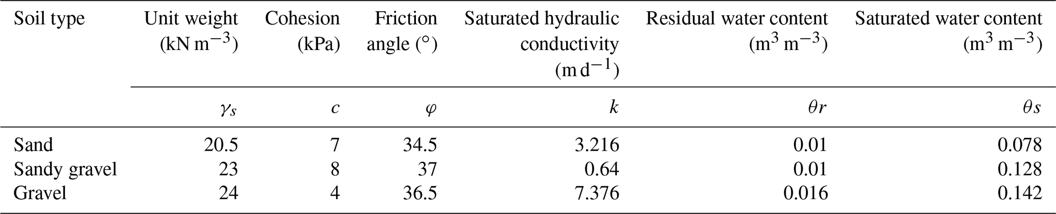
The mechanical and hydraulic soil properties employed in this model are listed in Table 1 and were obtained from Dann et al. (2009) and Aqualinc Research Limited (2007). We modelled two scenarios based on the available rainfall data (see Sect. 4.4). The first is a 3 d long intense rainfall event ((I-D)₃) covering the period 20–22 July 2017. The second is a 14 d period with occasional, low-intensity rain ((I-D)₁₄) between 21 June and 4 July 2017. Each scenario is modelled for two sandy gravel slopes with different permeabilities – one with a 0.5 m thick sand lens and the other with a 0.5 m thick gravel lens. Both lenses are located at a height of 5 m above sea level. Lateral water inflow and surface water infiltration were estimated from the hydrological model in Micallef et al. (2020). Slope stability modelling and groundwater analyses were carried out using the Slide2 software package by Rocscience.

Table 1 Mechanical and hydraulic soil properties used in slope stability modelling.

4 Results

4.1 Gullies along the Canterbury coast – distribution and morphology

We have mapped 315 gullies (locally also known as dongas) along 70 km of the Canterbury coastline (mean of 4.5 gullies per square kilometre of coastline). The spatial distribution of the gullies is clustered (nearest-neighbour ratio of 0.33, with a z score of −22.67 and a p value of 0); the majority of the gullies are located between the Rakaia and Rangitata rivers (Fig. 1a), particularly in the vicinity of the Ashburton River. The heads of many gullies connect to shallow, relict meandering channels (Fig. 2a). Some of these channels are visible in aerial photographs, in spite of the terrain having been worked by farmers (Fig. 2b).

Figure 2 (a) Slope gradient map of the study area. Black arrows indicate relict infilled channels. (b) Aerial photograph of Coldstream on the Canterbury coast (source – Environment Canterbury). Black arrows indicate relict infilled channels. Yellow arrows indicate gullies. Location shown in Fig. 1a. (c) Plot of length vs. width for gullies mapped along the Canterbury coastline.

In plan view, the gullies are predominantly linear to slightly sinuous (sinuosity of 1–1.3) and characterised by a concave head. In profile, the gullies have linear, gently sloping (2–10^∘) axes, with a concave break of slope separating the axis from a steep (up to 70^∘) head. In cross section, the gullies are U-shaped, with walls of up to 70^∘ in slope gradient. The gullies are between 5 and 1134 m long (mean of 116 m) and between 3 and 637 m wide (mean of 56 m). Gullies generally exhibit a constant width with a distance upslope. They have a length-to-width ratio that varies between 1 and 7.9, with a mean of 2 (standard deviation of 0.89; Fig. 2c).

4.2 Field site observations

In May 2017, our study area hosted 33 gullies that vary between 15 and 600 m in length (Figs. 1b, 3a). During the site visits, we did not encounter evidence of surface flow. However, the middle to lower sections of the gully walls and cliffs were consistently wet. These sections were also characterised by failure scars and alcoves, particularly above the sandy lenses. Alcoves were also encountered at the base of gully heads, where they were wet and up to 1 m deep (Fig. 3e). Some sandy layers outcropping across the cliff face hosted tunnels (Fig. 3c–d). Above these tunnels, theatre-shaped scars with a shallow and narrow gully at their base were observed (Fig. 3c). At the base of the scars, the gully heads and some gully mouths, we encountered mass movement debris that was occasionally intact and that predominantly consisted of gravel, sandy gravel and loess (Fig. 3c, h). Gullies have gravel-covered irregular floors. Whereas the smaller gullies have a U-shaped cross section, the three longest gullies have gently sloping V-shaped cross sections, with loess draping their walls (Fig. 3f). Sandy and clean gravel layers outcropping within the gullies were wet; the former appeared weathered, whereas the latter were coated by Fe and Mn (Fig. 3g). Fences were locally seen suspended across a number of gullies (Fig. 3b).

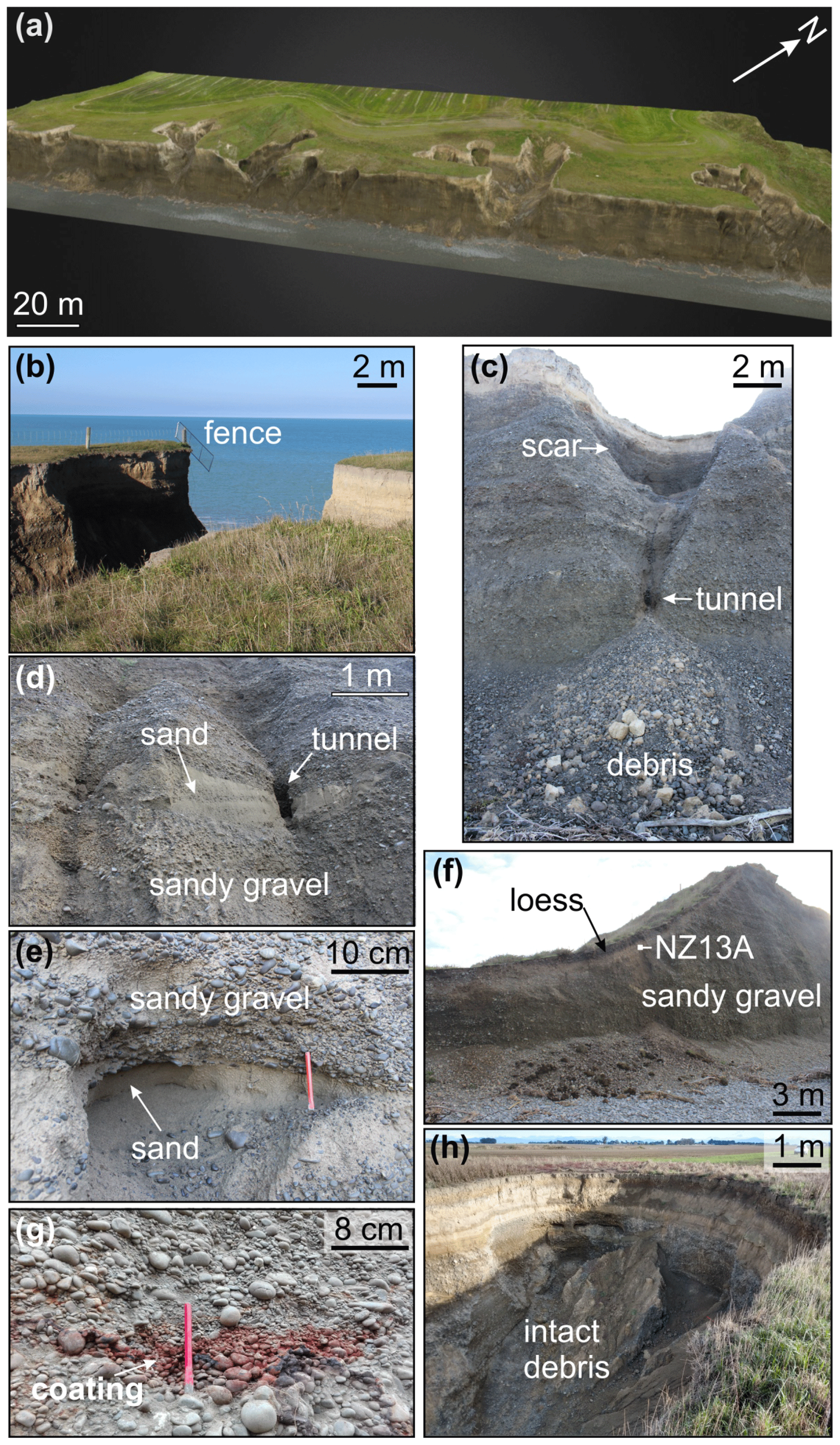
Figure 3 (a) Orthophoto map of part of the study area draped on a 3D digital elevation model. Location shown in Fig. 1b. (b–h) Photographs of features of geomorphic interest taken at the study area. The location of sample NZ13A is shown in (f).

4.3 Infrared stimulated luminescence ages

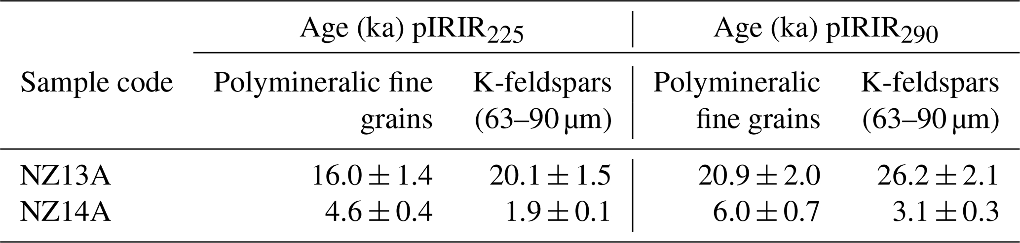
Four sets of infrared stimulated luminescence ages are presented in Table 2. The pIRIR₂₉₀ ages are higher than the ages obtained by applying the pIRIR₂₂₅ protocol. The cause of this difference is not yet fully understood, although it can partially be attributed to the results of the dose recovery test and the poor bleachability of the pIRIR₂₉₀ signals compared to pIRIR₂₂₅ signals (Buylaert et al., 2011). Considering that no anomalous behaviour of the investigated signals was observed (see the Supplement), we are unable to explain the overestimation of the K-feldspar ages compared to the polymineralic fine-grain ages in the case of NZ13A, especially since the opposite behaviour is observed in the case of sample NZ14A. However, considering a 95 % confidence level, infrared-stimulated luminescence ages obtained using different methods broadly overlap, with the only exception being the pIRIR₂₂₅ ages obtained on K-feldspars on sample NZ14A, which we regard as an outlier.

Table 2 Summary of the pIRIR₂₂₅ and pIRIR₂₉₀ ages obtained on polymineralic fine grains (4–11 µm) and coarse K-feldspars (63–90 µm). The infrared stimulated luminescence ages were determined considering 15 % water content. Uncertainties are given at 1σ, with a 68 % confidence level. Further details are available in the Supplement.

4.4 Morphological changes

4.4.1 Short-term morphological changes

By comparing the orthophotos and digital elevation models generated from the UAV data acquired during the various site visits between May and October 2017, we document the formation of three new gullies (up to 30 m long; Figs. 4e–f) and the enlargement of 30 gullies (primarily by elongation and occasionally by widening and branching; Fig. 4a–d). The new gullies formed at locations where there was a small landslide scar in the middle of the cliff. There was no change in form in three of the gullies. Figure 5 shows the total area eroded between surveys (which amounts to approximately 3273 m²), the daily precipitation and the associated changes in water table height. Only three surveys recorded gully erosion. A total of two of these surveys happened soon after rainfall events of > 40 mm in 1 d (Fig. 5). The most important of these covers the period between 15 and 23 July 2017 when 95 % of the material was removed and the three new gullies were formed (Figs. 4–5). During this period, a total of 153 mm of rain fell (up to 120 mm on 21 July 2017 alone, which was the most intense rainfall event since 1936), resulting in a 1.5 m rise in the water table. A third survey occurred 6 d after the 21 July 2017 storm, with 22 mm of rain falling in 1 d. The material eroded from the gullies was deposited at the base of the cliffs as gravel cones, which were remodelled by debris flows during the ensuing precipitation events and subsequently disappeared from the orthophotos.

Figure 4 (a–d) Orthophotographs of the study area at the start and end of the UAV surveys, ordered from southwest to northeast. Red lines mark eroded areas. Location shown in Fig. 1b. Orthophotographs from a part of the study area on (e) 15 July 2017 and (f) 23 July 2017. Location shown in (b).

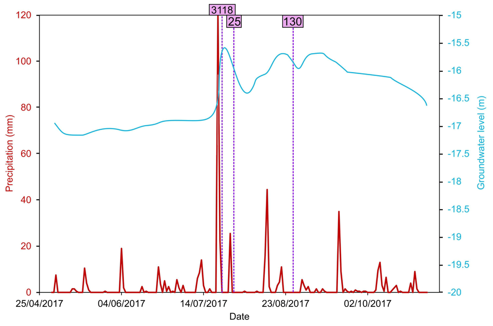
Figure 5 Daily precipitation (for Ashburton District Council) and groundwater level records (from a well located 10 km northeast of the study area) for the period 1 May to 31 October 2017 (source – Environment Canterbury). The pink lines mark the surveys during which gully erosion was observed (the value in the pink box corresponds to the eroded area in square metres; uncertainty is 0.25 m²).

4.4.2 Long-term morphological changes

For the period 2004–2015, we used satellite imagery to map the formation of six new gullies and the elongation of 22 gullies. A total of 18 of these erosion episodes are recorded in the image taken on 26 August 2013 (Fig. 6a). This follows a major rainfall event between 16 and 23 June 2013, when 171 mm of rain fell in 7 d (with up to 51 mm falling in 1 d; Fig. 6b). The other erosion episodes include the five gullies eroded by 28 March 2009, after a storm of 46 mm d⁻¹ on 31 July 2008, and the five gullies eroded by 19 October 2015, after a storm of 43 mm d⁻¹ on 19 June 2015.

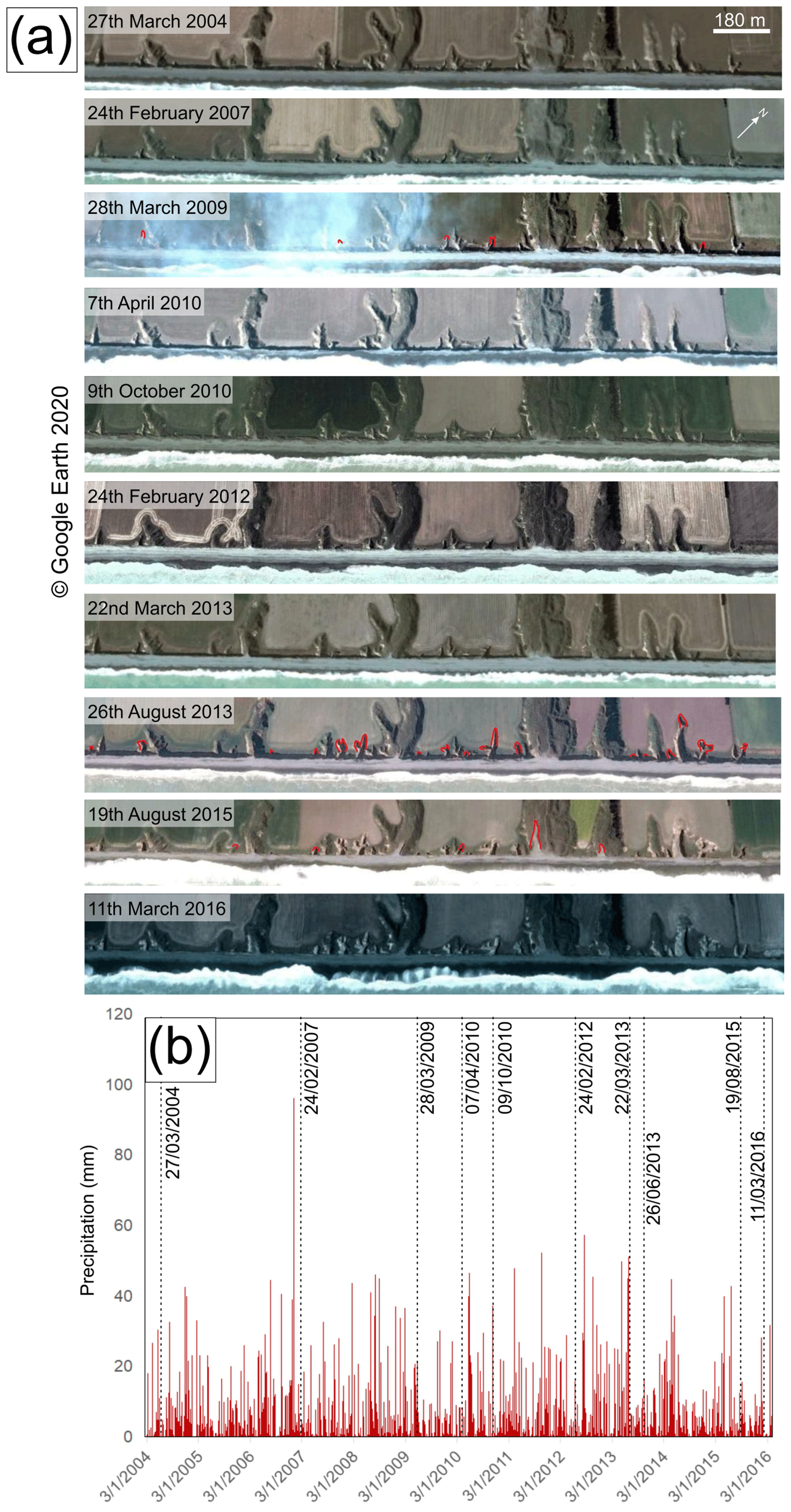
Figure 6 (a) Satellite imagery of the study area between the 27 March 2004 and 11 March 2016 (source – © Google; Maxar Technologies). Eroded areas are marked by red lines. (b) Daily precipitation record for this period for Ashburton District Council (source – Environment Canterbury). The dates on which the satellite imagery was collected are denoted.

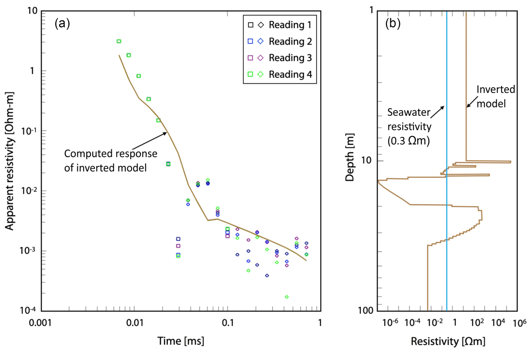
Figure 7 A 1D inversion result for G-TEM data, shown as squares and diamonds (representing positive and negative responses, respectively), at a station located 6 m from start of profile May15-1. (a) The computed resistivity depth profile displayed as a curve passing through data points. (b) The best-fit model is marked as the brown line, while the light blue line is the inferred seawater resistivity.

4.5 Geophysical data

The location of the G-TEM transects is shown in Fig. 1b. An attempt was made to invert the G-TEM slingram-mode responses with 30 m TX–RX offset, using a 1D Occam inversion. A representative inversion result is shown in Fig. 7. The resistivity model is presented in Fig. 7b, whereas the corresponding model response with the actual data points is shown in Fig. 7a. The best-calculated smooth depth profile clearly does not fit well with the measured signal, and there is excessive structure in the ∼ 10–20 m depth range, including the very low resistivity layer (∼ 10⁻⁴ Ωm) at depths in excess of ∼ 12–15 m. The resistivity values between 40 and 100 m depth are lower than sea water resistivity (0.3 Ωm), which is not reasonable. The inability to fit a 1D model to the slingram responses suggests that the geoelectrical subsurface structure is strongly heterogeneous within the footprint of the G-TEM transmitter. As a result, we cannot trust 1D inversions of the slingram-mode data in such a 3D geological environment. We did not try to use the 1D inversion software to further analyse and interpret the G-TEM data. However, even though the individual slingram-mode responses cannot be fitted reliably by a 1D model, we can still analyse the lateral changes in the observed response curves along the slingram profiles to reveal information about subsurface heterogeneity; this is elaborated on below.

Instead of performing 1D inversions, we present time gate plots for all three transects. A time gate plot is defined as a graph of the observed G-TEM voltage response, evaluated at a particular time gate, as a function of a position along a profile. Time gate plots are a useful alternative for exploring the lateral variability in the G-TEM response along a profile in the event that the sounding curves at individual stations cannot be fitted with 1D models. It is presumed that the variability in a time gate plot is correlated with lateral heterogeneity in the subsurface geoelectrical structure, since a 1D Earth structure would yield no spatial variability in a time gate plot. In general, due to lengthy signal-averaging times, ambient electromagnetic noise from the environment adds a very small contribution to TDEM responses, such that any along-profile variations are likely caused by geological heterogeneity. However, there is not a straightforward relationship between the magnitude of the TDEM voltage at any given time gate and the resistivity within a particular subsurface volume. The situation becomes more complicated since the true Earth is characterised by multiscale heterogeneity, such that spatial variations in the geology at all length scales superimpose their individual responses on one another to produce the final overall TDEM response that is measured. Thus, any analysis of the spatial variability in a time gate plot, while informative, is largely qualitative and indicates only a first-order spatial distribution of causative subsurface structures.

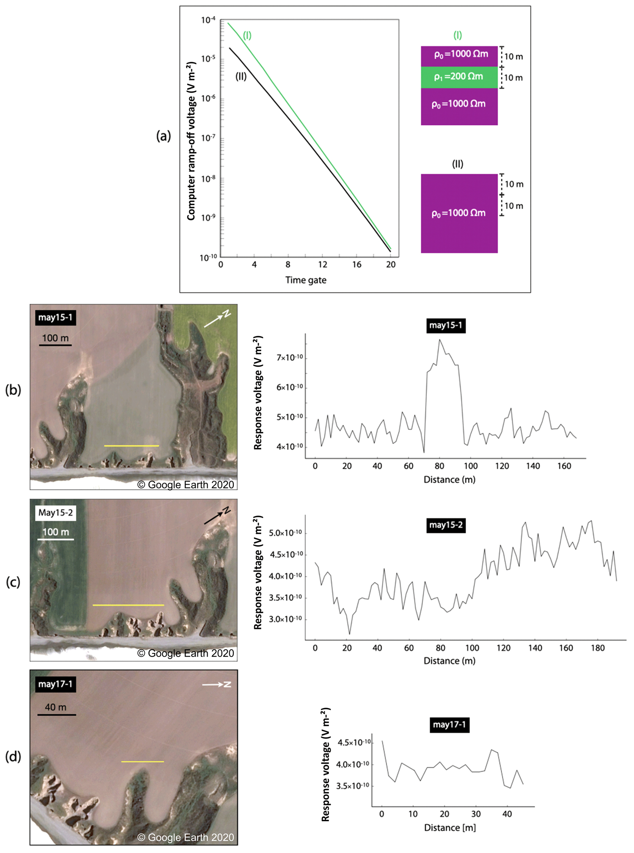
Figure 8 (a) G-TEM slingram response for an electrical model (I), containing a conductive zone at a depth of 10–20 m, and for a model (II), without the conductive zone. First time gate profiles of G-TEM slingram transects of (b) May15-1, (c) May 15-2 and (d) May17-2 are shown. The yellow line marks a slingram transect, the length of which can be determined from the scale bar. Source of background imagery – © Google; Maxar Technologies.

Specifically, the amplitude of the G-TEM slingram response (in units of 10⁻¹⁰ V m⁻²) at the first time gate is plotted as a function of the station number along a profile. Figure 8a displays a 1D model (I) that contains a conductive layer of 200 Ωm between a 10 and 20 m depth in a homogeneous 1000 Ωm background. The 1D model (i) is motivated by the inversion results of deep-penetrating 40 × 40 m TX loop TDEM soundings carried out on top of the cliffs several tens of metres inland (Weymer et al., 2020), which revealed such a conductive zone at these depths. Unlike the slingram profiles, the deeper-penetrating, larger-loop sounding curves are readily fitted by a 1D model. This model generates a G-TEM slingram response that has a substantially larger ramp-off voltage amplitude at all time gates than the model does (ii) without the conductive layer, as shown in Fig. 8a. Thus, we regard an enhancement in the response at the first time gate as indicative of a conductive zone at depth beneath the slingram station. The spatial analysis of the time gate plots is not a conventional approach in time domain electromagnetics, but it is somewhat analogous to the spatial analysis of the apparent resistivity profiles in frequency domain electromagnetics using terrain conductivity meters (e.g. Weymer et al., 2016). This is based on the idea that the G-TEM response at a fixed time gate carries information similar to that of a terrain conductivity meter response at a fixed frequency.

The first time gate profile of transect May15-1 is located upslope of small but recently eroded gullies (Fig. 8b). In this figure, the first time gate profile is a plot as a function of the distance along the transect of the G-TEM ramp-off voltage at time gate number 1, which is the first sampled point of the transient response immediately after the TX current has been switched off. Near the middle of this transect, there is a distinctive peak that is much higher than the background. The peak is ∼ 20–30 m wide, and it appears in a similar fashion on each of the gates 1 through 7 (not shown here), although it cannot be clearly observed after gate 7. Transect May15-2 is located upslope of recently eroded gullies in the southwest and relatively less active gullies in the northeast of the investigated area (Fig. 8c). Lateral variations are evident along the 192 m length of the profile. The high-amplitude response at the start of the profile (going from the southwest to the northeast) is followed by a drop in amplitude near the midpoint of the profile, after which there is continuous fluctuation at a lower amplitude until the end of the profile. The time gate plots for gates 2 to 7 remain similar in shape to that of the time gate 1 plot and, hence, are not shown. After time gate 7, the time gate plots start to lose coherence due to the low signal-to-noise ratio of the decaying RX voltage at late times after TX ramp off. The G-TEM slingram profile May17-2 was acquired upslope of the tributary of a large gully covered by mature vegetation (Fig. 8d). As shown in Sect. 4.4, the size and location of this gully have been persistent over recent years, in contrast to the neighbouring, smaller gullies that are under active development. Transect May17-2 shows a lower amplitude response in comparison to the previous two transects (Fig. 8).

Based on all three profiles, a general observation that can be made is that the first time gate amplitude of the slingram response is higher upslope of the more recently active gullies.

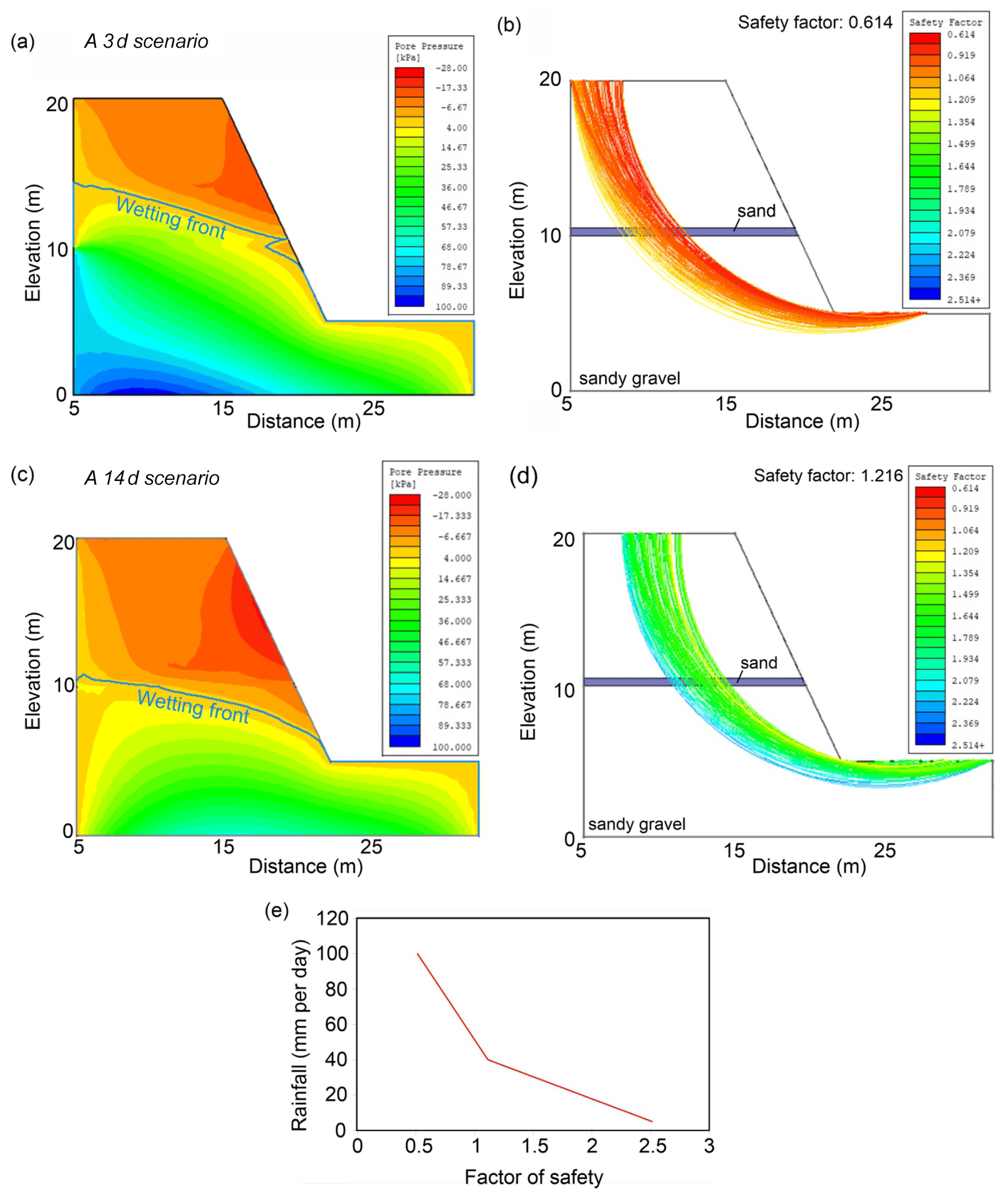
Figure 9 Model results for a sandy gravel slope with a sand lens. Estimated pore water pressure and factor of safety after 3 d for the first scenario ((I-D)₃) (a–b) and 14 d for the second scenario ((I-D)₁₄) (c–d). (e) Plot of rainfall intensity vs. factor of safety for the for first scenario ((I-D)₃) for the slope with sand lens. The results shown are for the end of the simulation for each scenario.

4.6 Slope stability modelling

4.6.1 Slope with sand lens

The factor of safety of the slope prior to any rainfall event was 2.514. During the first scenario ((I-D)₃), the factor of safety decreased to 1.371, due to undermining by tunnelling associated to high pore pressures within the sand lens, and then to 0.614, as a result of a decrease in the shear strength of the lower slope material due to an increase in pore pressure (Fig. 9a–b). A rainfall intensity of 40 mm d⁻¹ is required to bring the factor of safety below 1 (Fig. 9e), and up to 4.4 m³ of water is estimated to have seeped out of the cliff face to erode 1650 m³ of material. In the case of the second scenario ((I-D)₁₄), changes in pore water pressure did not result in either tunnelling or slope failure. This only resulted in a decrease in the effective stress and in the factor of safety (1.216; Fig. 9c–d).

4.6.2 Slope with gravel lens

The factor of safety of the slope prior to any rainfall event is 1.793. For the first scenario ((I-D)₃), the factor of safety decreased to 1.166, and neither tunnelling nor slope failure occurred (Fig. 10a–b). In the case of the second scenario ((I-D)₁₄), the outcome is the same, with the factor of safety decreasing to just 1.588 (Fig. 10c–d). The factor of safety does not reach a value lower than 1 for rainfall intensities of up to 120 mm d⁻¹ (Fig. 10e).

Figure 10 Model results for sandy gravel slope with gravel lens. Estimated pore water pressure and factor of safety after 3 d for the first scenario ((I-D)₃) (a–b) and 14 d for the second scenario ((I-D)₁₄) (c–d). (e) Plot of rainfall intensity vs. factor of safety for the for first scenario ((I-D)₃. The results shown are for the end of the simulation for each scenario.

5 Discussion

Gullies are characteristic landforms along the Canterbury coast (Fig. 1a). They are an important driver of coastal geomorphic change and loss in agricultural land. In the following sections, we integrate field observations with the modelling results to infer how coastal gullies are formed by groundwater erosion, the role that lithology and permeability play in gully initiation and evolution and the temporal scale of gully formation.

5.1 Coastal gully formation by groundwater-related processes

The Canterbury gullies initiate and evolve via two types of groundwater-related processes. The first process is the seepage erosion of sand, which leads to the formation of alcoves and tunnels. This inference is based on the exclusive occurrence of tunnels in sandy layers at the study site (Fig. 3c–e). Seepage erosion lowers the overall factor of safety of the slope, as demonstrated by slope stability model results for the slope with sand lens scenario, and is a precursor to the second process, which is slope failure (Fig. 3c). Site observations (Fig. 3h), the UAV data (Fig. 4) and satellite imagery (Fig. 5) show that gullies primarily evolve by retrogressive slope failure, which results in the elongation of the gullies and, to a lesser extent, widening and branching along the gully walls. According to the slope stability model in Fig. 9a, up to 4.4 m³ of seepage water is required to erode 1650 m³ of sediments, which contrasts with the inference by Howard (1988) that 100–1000 times more water than volume of eroded sediment must be discharged in order to create a sapping valley. We infer that wave erosion is responsible for the removal of the failed material at the gully mouths and the base of the cliff. Isotropic scaling of length with width (Fig. 2c) suggests that gully planform shape is generally geometrically similar at consecutive stages of evolution.

5.2 Influence of geological/permeability heterogeneity on gully formation

Two factors control the location of gullies. The first factor is the occurrence of sand lenses across a sandy gravel cliff face. This geological framework is conducive to alcove formation, tunnelling and slope failure (Fig. 3c–e). The higher permeability of the sand and clean gravel lenses, in comparison to the surrounding sandy gravel (Table 1), facilitates faster water transfer to the cliff face; this is also corroborated by the weathering in the sandy layers and Fe and Mn deposits in the clean gravel layers (Fig. 3g). Alcoves and tunnels only form in the sand lenses; however, the latter develop higher pore pressures, and sand is easier to entrain and remove in comparison to clean gravel in view of its lower shear strength (Table 1). Slope failure only occurs in sandy gravel slopes with sand lenses (Figs. 9–10). The higher pore pressure developed in the sand lenses is transferred to the sandy gravel slopes, resulting in a larger decrease in the shear strength and higher water table in comparison to the sandy gravel slope with gravel lens.

The second factor is a hydraulically conductive zone upslope of the gully. This inference is supported by the following observations: (i) braided river channel infills, which tend to comprise highly permeable, coarse-grained materials (Moreton et al., 2002), lead into the gullies' heads (Fig. 2a–b); (ii) clustered distribution of gullies between the two braided rivers with the highest flow rates (Rakaia and Rangitata rivers; Environment Canterbury, 2019; Fig. 1a); (iii) geophysical observations (Fig. 8). With regards to the G-TEM slingram time gate plots (Fig. 8), we interpret the higher-amplitude responses on the time gate 1 plots that are preferentially located upslope of recently active gullies as being zones of relatively high electrical conductivity in the subsurface at depths of ∼ 10 m. These zones are suggestive of buried groundwater conduits made up of gravel and/or sandy units (Weymer et al., 2020) or tunnels formed by subsurface groundwater flow in sand units. Further analysis of the G-TEM data, including 2D modelling and inversion, is required to ascertain the subsurface hydraulic geometry responsible for the along-profile amplitude variations. This is elaborated on in the Supplement. The above observations confirm the importance of spatial variations in hydrogeological properties as a factor controlling the location of a gully. This had initially been suggested by Dunne (1990) and has been documented for gullies in bedrock environments (Laity and Malin, 1985; Newell, 1970). Development of gullies downslope of permeable conduits may also explain why most of the erosion entails the elongation of existing gullies rather than formation of new ones (Figs. 4, 6). It also agrees with the results of the experimental modelling by Berhanu et al. (2012), which suggest that channels grow preferentially at their tip when the groundwater flow is driven by an upstream flow. If seaward-directed groundwater conduits are responsible for the location of gullies, the G-TEM results predict that, along the Canterbury coast, we should generally observe active gully development downslope of peaks in slingram time gate plots. If this is the case, G-TEM could be used to identify the locations of incipient and even future gully development.

5.3 Temporal scale of gully formation

Morphological changes derived from the time series of UAV data (Figs. 4–5) and satellite imagery (Fig. 6), and the observations of suspended fences across gullies (Fig. 3b), suggest that gully formation is rapid (on daily timescales) and recent (< 3 years ago). It is an episodic process that occurs after a threshold is exceeded. This threshold entails a rainfall intensity of > 40 mm d⁻¹, which occurs once every 227 d on average. The threshold value is based on UAV and satellite imagery observations, which show that gullies form after rainfall events, with an intensity higher than 40 mm d⁻¹ (Figs. 5, 6), and the plot of the factor of safety with rainfall intensity from the slope stability model for the first scenario ((I-D)₃ for the slope with sand lens (Fig. 9). The erosion rate documented in our study area is up to 30 m d⁻¹ (Fig. 4e-f), which is the highest rate documented for gullies formed by groundwater so far.

The majority of the gullies in our study area have shown evidence of erosion in the past 11 years (Figs. 4, 6). The luminescence-dating results (Table 2), however, suggest that the two largest gullies have largely been inactive during at least the last 2 ka; recent erosion is only documented in small gullies located in the central section of their mouths (Figs. 4, 6). This contrasts with the inference by Schumm and Phillips (1986) that they were formed by the spillage of water from swamps behind the cliffs in the 19th century. We therefore propose that the short gullies (< 200 m in length) are recently active features, whereas the largest gullies are relict features that formed as a result of higher groundwater flow, and possibly surface erosion, in the past. The age of sample NZ13A suggests that this may have occurred during the Last Glacial Maximum. Such a difference in age, and possibly formation process, between gullies of different lengths may explain the different cross sectional shape and higher scatter in the plot of length vs. width for the longer gullies (Fig. 2c).

6 Conclusions

Gully erosion is a prevalent process shaping the Canterbury coast of the South Island of New Zealand. In this study, we have integrated field observations, luminescence dating, multi-temporal UAV and satellite data, time domain electromagnetic surveying and slope stability modelling to constrain the controlling factors and temporal scales of gully formation. Our results indicate that gully development in sandy gravel cliffs is a groundwater-related, episodic process that occurs when rain falls at intensities of > 40 mm d⁻¹. At the study area, such rainfall events occur at a mean frequency of once every 227 d. Gullies have been developing, primarily by elongation, in the last 11 years, with the latest episode dating to 3 years ago. Gullies form within days, and erosion rates can reach values of up to 30 m d⁻¹. Gullies longer than 200 m, on the other hand, appear to be relict features that formed by higher groundwater flow and surface erosion > 2 ka ago. The key processes responsible for gully development are the formation of alcoves and tunnels in sandy lenses by groundwater seepage erosion, followed by retrogressive slope failure. The latter is a result of undermining and a decrease in shear strength due to excess pore pressure development in the lower part of the slope. The location of the gullies is controlled by the occurrence of hydraulically conductive zones, which comprise relict braided river channels, and possibly tunnels, and sand lenses exposed across the sandy gravel cliff. We also show that gully planform shape is generally geometrically similar at consecutive stages of evolution. The outcomes of our study can improve the reconstruction and prediction of an overlooked geohazard along the Canterbury coastline.