the Creative Commons Attribution 4.0 License.
the Creative Commons Attribution 4.0 License.
 | 04 Apr 2022
Comparing the transport-limited and ξ–q models for sediment transport
Here I present a comparison between two of the most widely used reduced-complexity models for the representation of sediment transport and deposition processes, namely the transport-limited (or TL) model and the under-capacity (or ξ–q) model more recently developed by Davy and Lague (2009). Using both models, I investigate the behavior of a sedimentary continental system of length L fed by a fixed sedimentary flux from a catchment of size A0 in a nearby active orogen through which sediments transit to a fixed base level representing a large river, a lake or an ocean. This comparison shows that the two models share the same steady-state solution, for which I derive a simple 1D analytical expression that reproduces the major features of such sedimentary systems: a steep fan that connects to a shallower alluvial plain. The resulting fan geometry obeys basic observational constraints on fan size and slope with respect to the upstream drainage area, A0. The solution is strongly dependent on the size of the system, L, in comparison to a distance L0, which is determined by the size of A0, and gives rise to two fundamentally different types of sedimentary systems: a constrained system where L<L0 and open systems where L>L0. I derive simple expressions that show the dependence of the system response time on the system characteristics, such as its length, the size of the upstream catchment area, the amplitude of the incoming sedimentary flux and the respective rate parameters (diffusivity or erodibility) for each of the two models. I show that the ξ–q model predicts longer response times. I demonstrate that although the manner in which signals propagates through the sedimentary system differs greatly between the two models, they both predict that perturbations that last longer than the response time of the system can be recorded in the stratigraphy of the sedimentary system and in particular of the fan. Interestingly, the ξ–q model predicts that all perturbations in the incoming sedimentary flux will be transmitted through the system, whereas the TL model predicts that rapid perturbations cannot. I finally discuss why and under which conditions these differences are important and propose observational ways to determine which of the two models is most appropriate to represent natural systems.
- Article
(9120 KB) - Full-text XML
-
Supplement
(911 KB) - BibTeX
- EndNote


Sedimentary basins contain the record of Earth's past tectonic and climatic histories. To untangle this record, scientists often rely on the use of numerical models that simulate the physical processes controlling sediment production, transport and deposition. Models are commonly used to characterize the response of sedimentary systems to external forcing in the source area (change in tectonic uplift rate or in rainfall intensity) or in the depositional environment (variations in sea level). In particular whether perturbations can propagate across so-called “source-to-sink” systems remains an open question (Romans et al., 2016; Tofelde et al., 2021) that models have attempted to answer (Castelltort and Van Den Driessche, 2003; Simpson and Castelltort, 2006; Armitage et al., 2011, 2013; Mouchené et al., 2017).
Traditionally, sediment transport has been represented using a nonlinear diffusion equation assuming that the process is limited by the transport capacity of rivers (the main transport agents) that is assumed to be proportional to slope and discharge and to other factors, including grain size (Henderson, 1966). I will name this model the transport-limited or TL model. Recently Davy and Lague (2009) introduced a new model (which they named the ξ–q model) to represent the competition between sediment production (erosion), transport and deposition in fluvial systems. Improving on the work from previous authors (Kooi and Beaumont, 1994), their main purpose was to produce a model that could account for the transition from detachment-limited to transport-limited behaviors of mountain channels. In recent years, the model has also been used to study sedimentary systems outside of the orogenic area, i.e., in purely depositional settings (Carretier et al., 2016; Shobe et al., 2017; Yuan et al., 2019), and this has led to attempts (Guerit et al., 2019) to quantify the value of the main model parameter, ξ, originally described as a characteristic transport length that depends on discharge but later remapped into the inverse of a rate (Carretier et al., 2016) or a dimensionless number (the Θ parameter of Davy and Lague, 2009 or the G parameter of Yuan et al., 2019).
Although Davy and Lague (2009) described the behavior of their model in great detail, including the conditions that favor transport-limited over detachment-limited behavior or the response time of a system obeying their formulation to both long- and short-term variations in uplift rate, the behavior of the model in a purely depositional environment has not been studied thoroughly. I believe it is, however, essential that such an analysis be made in order to validate this model or, at minimum, to understand its limits of applicability and ultimately adequately interpret the predictions that might be made by using it in future work. This is what I propose to do here, in addition to comparing its predictions to the traditional nonlinear diffusion approach or TL model.
It is important, however, to keep in mind that the ξ–q model behavior asymptotically tends towards that of the TL model for small values of the depositional length ξ or, more correctly, for large values of the Θ dimensionless number introduced by Davy and Lague (2009) or the G-factor introduced by Yuan et al. (2019). Even though one of them, the ξ–q model, “contains” the other, I will compare the two models as independent of one another rather than comparing the effect of an infinite value of the Θ dimensionless number, mostly for practical reasons (as we do not know how large a value of Θ to use for the ξ–q model to behave exactly like the TL model) but also because the TL model existed before its generalization was introduced.
Although the purpose of this work is to compare the general behavior of two sediment transport models, I will focus on sedimentary systems that develop at the foot of an orogenic area, more precisely the fan and neighboring alluvial plain. The idea is to study a system that is familiar to sedimentologists but relatively simple in its setting, such that the intrinsic behaviors of the two models can be efficiently analyzed and compared to observational constraints.
2.1 The two models
Traditionally, the transport of sediment by rivers has been modeled using the transport-limited (or TL) model (Henderson, 1966). In the TL model a river is assumed to transport sediment at its transport capacity. The transport capacity or optimum flux of sediment, q (expressed in m2 yr−1), is assumed to be proportional to local topographic slope, S (expressed in m m−1), and specific discharge, qw (expressed in m2 yr−1), raised to some powers, m+1 and n:
Specific discharge will be assumed to be the product of upstream drainage area, A (expressed in m2), by net precipitation rate ν (dimensionless) relative to some reference value that is commonly inserted into a rate parameter or transport coefficient, Kd (expressed in m1−m yr−1), divided by the floodplain width, w (expressed in m) to yield the following equation:
Conservation of mass leads to the following evolution equation for surface elevation, h (expressed in m):
where x is the direction of flow in the river (expressed in m) and t is time (expressed in years), noting that . Note that I have assumed that there is only one material that is transported, deposited and potentially eroded, such that I do not need to worry about density differences between what is transported and eroded or deposited off the riverbed. I will call Eq. (3) the TL equation.
The ξ–q model (Davy and Lague, 2009) assumes that the rate of change of topographic height is the sum of two terms, one representing erosion and the other deposition. Erosion rate, , is assumed to be governed by the stream power law (SPL) and thus proportional to the product of specific discharge and slope raised to some power (Howard and Kirby, 1983; Whipple and Tucker, 1999):
while deposition rate, , is assumed to be proportional to the ratio of upstream-integrated sedimentary flux and a deposition length that depends on specific discharge, ξ(qw) (Davy and Lague, 2009):
I will follow Davy and Lague (2009) and assume that ξ is given by
where vs is the net settling velocity of sediment particles (i.e., taking into account turbulence) and d* a dimensionless parameter characterizing the distribution of particles in the river (it is the ratio of the water column height by the thickness of the actively transporting layer). This leads to the following evolution equation:
where Kf is the erodibility coefficient (that has units of m1−m yr−1) and G is a dimensionless parameter defined as follows:
where ν0 is mean precipitation rate. The parameter G was proposed by Yuan et al. (2019) and is equivalent to the parameter Θ introduced by Davy and Lague (2009). In their implementation of the ξ–q model, Carretier et al. (2016) used a parameter relating the depositional length to specific discharge that they call ζ and has the dimensions of the inverse of a velocity [T L−1]. It is related to the dimensionless parameter, G, used here by the following relationship:
Davy and Lague (2009) estimated that Θ (or G) is likely to be greater than or equal to one, depending on grain size, rainfall intensity and variability (Guerit et al., 2019). These authors used the change in channel slope at the orogenic front to estimate the value of G. Compiling observations from many sedimentary systems, they estimated that G must be in the range [1–2].
Note that in both Eqs. (3) and (7) I have assumed that the floodplain width, w, is constant, as has been done, for example, in Goldberg et al. (2021). As shown by Nardi et al. (2006), floodplain width varies as a weak function of drainage area, i.e., w∝Aθ, with θ≈0.2–0.3. However, one could consider w to be an averaged value of the floodplain width for the system under consideration and that its variation with drainage area or discharge is factored in the value of the exponent m, as commonly assumed.
2.2 Experimental setup
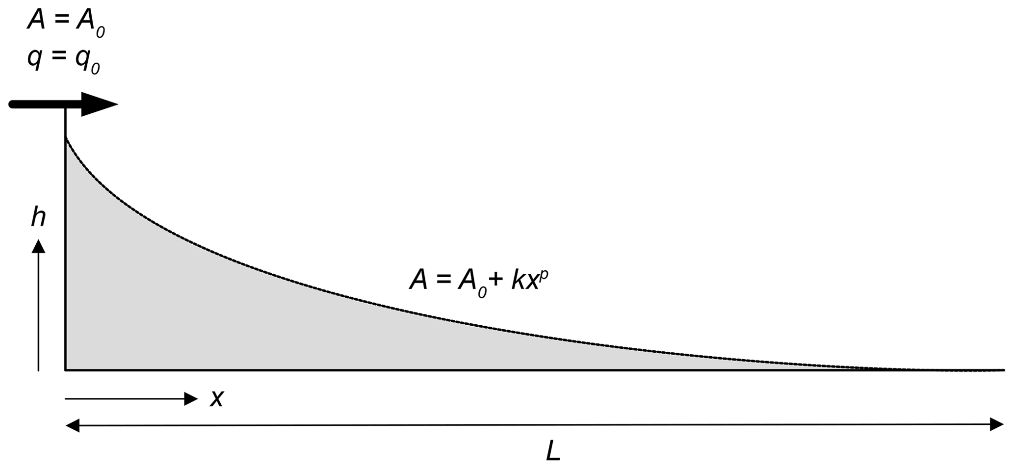
To compare the behavior of these two equations, I will use a very simple setup (Fig. 1) in which an initially flat (h=0) surface of length L accumulates sediment brought at a constant flux, q0, across its left-hand-side boundary at x=0. The drainage area will be assumed to obey Hack's law:
where A0 is the drainage area of the orogenic area where the river has its source, outside of the domain defined by . Assuming that p=2 leads to k being dimensionless.
The right-hand-side boundary, at x=L, is assumed to correspond to a base level (a large river or an ocean) such that its elevation remains nil through time. This yields the following boundary conditions:
for the TL equation and
for the ξ–q equation.
2.3 Numerical method used
I developed simple time-implicit finite-difference schemes to solve these equations numerically under the simplifying assumption that n=1 (see Appendix A for details).
3.1 Steady-state solution
Both equations share the same steady-state solution. Indeed, setting and ν=1 in Eqs. (3) and (7), one obtains the following
for the TL equation and
for the ξ–q equation, which yields the following expressions for the topographic elevation:
for the TL equation and
for the ξ–q equation. is the hypergeometric function.
The two equations have steady-state solutions that have the same form and are identical if/when GKd=Kf. This solution is shown in Fig. 2 for parameter values given in the caption. Its shape is determined by the ratio or , where is the linear size of the upstream catchment or orogenic area. In Fig. 3, I show three solutions corresponding to three different values of . In systems where the size of the depositional area is smaller than or equal to the size of the orogenic area (L≤L0), the depositional profile is quasi-linear (Fig. 3a and b). In the more general case where L>L0, the profile is made of two separate sections: in the section near the orogenic area defined by x<L0, the depositional profile is quasi-linear, while in the other section defined by x>L0, the profile is upwardly concave and progressively tapers towards base level (Fig. 3c).
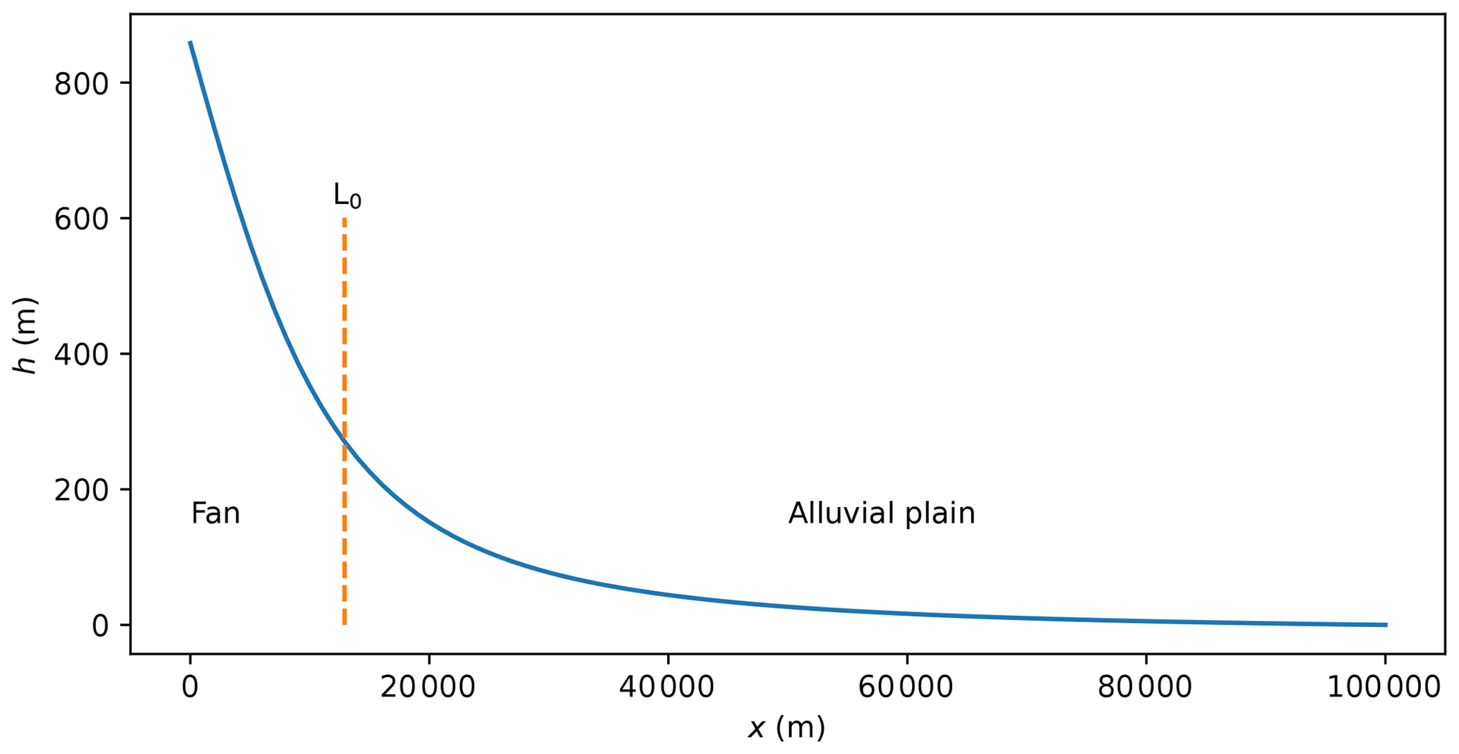
Figure 2Steady-state depositional profile obtained by solving both the ξ–q and TL equations using m1–2 m yr−1; G=1 yr m−1; m−2 m yr−1; w=104 m; m=0.4, n=1, L=100 km; A0=108 m2; k=0.6; p=2 and q0=10 m yr−1.
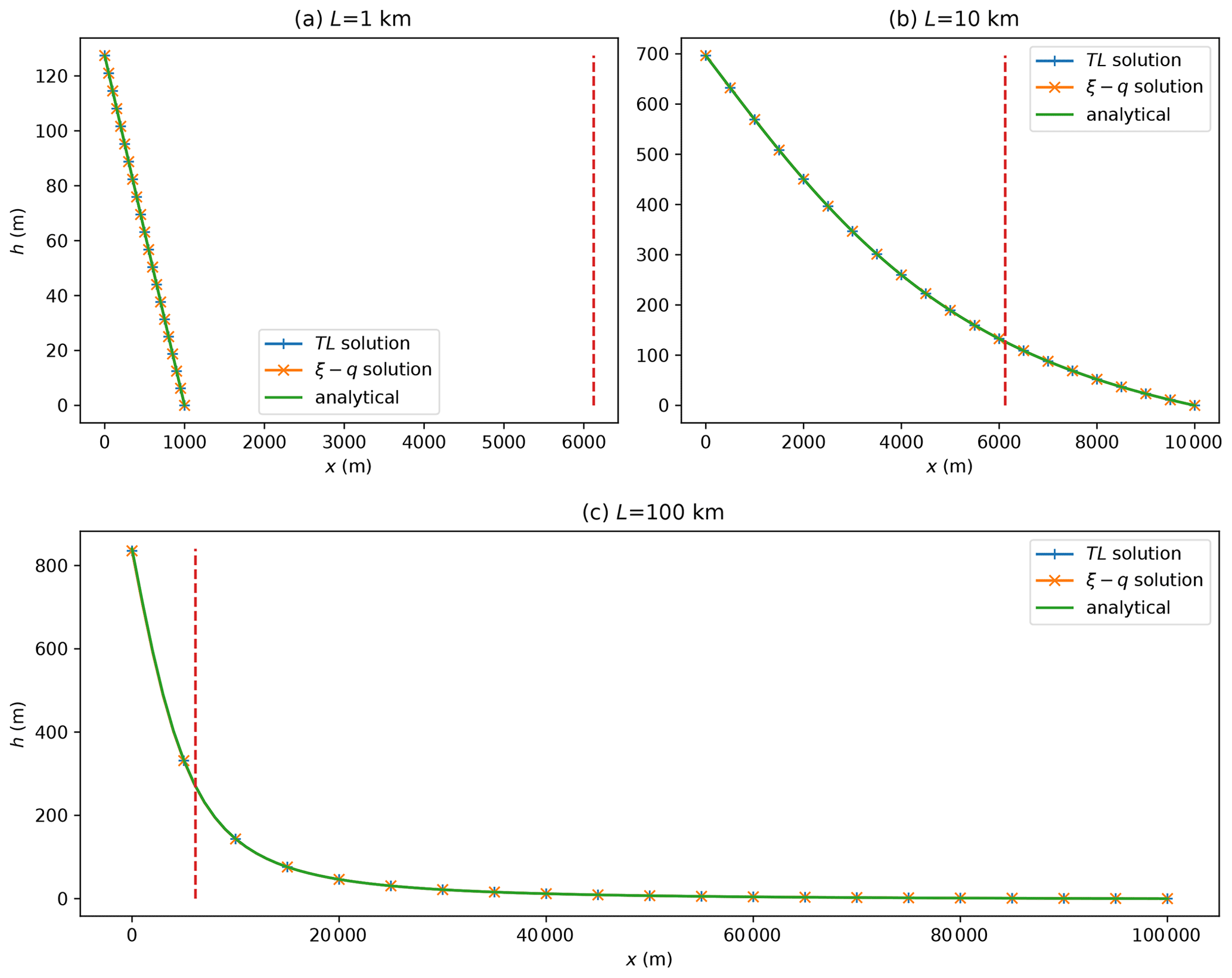
Figure 3Steady-state depositional profiles obtained by solving both the ξ–q and TL equations using three different values for the ratio ; all other parameters are identical to values used for the profile in Fig. 2. The dashed line represents the position of the length scale . Three curves are shown, corresponding to the analytical solution as described by Eqs. (15) or (16) and the two solutions obtained using the numerical methods described above.
This geometry is similar to what is observed in natural systems (Bull, 1977; Blair and McPherson, 2009; Bowman, 2019): in the most common situation where the depositional system is much longer than the orogenic system, i.e., L≫L0, the depositional system comprises a steep and constant slope fan, which connects to a much gentler slope alluvial plain; in cases where the depositional system is shorter than the orogenic system, such as next to a mountain neighboring an ocean, the depositional system is limited to a steep, linear (conic in two dimensions) fan. From here on, I take the convention to name the systems where L<L0 “constrained” systems, i.e., their short length relative to the length of the upstream orogenic area prevents them from building an alluvial plain, whereas those where L>L0 will be called “open” systems, i.e., as they are able to develop an alluvial plain at the foot of their fan.
We note that the parameters q0, Kf, G, w, Kd and A0 control the height of the depositional system but that its shape, i.e., where it transitions from a linear segment to a curved segment, only depends on the ratio of the depositional system size to the orogenic system size (length or area) .
The slope of the steady-state solution is given by
for the TL equation and
for the ξ–q equation.
The predicted steady-state slope of the fan system, i.e., at x=0, and alluvial plain, i.e., at x=L, are given by
respectively, for the TL equation and
for the ξ–q equation.
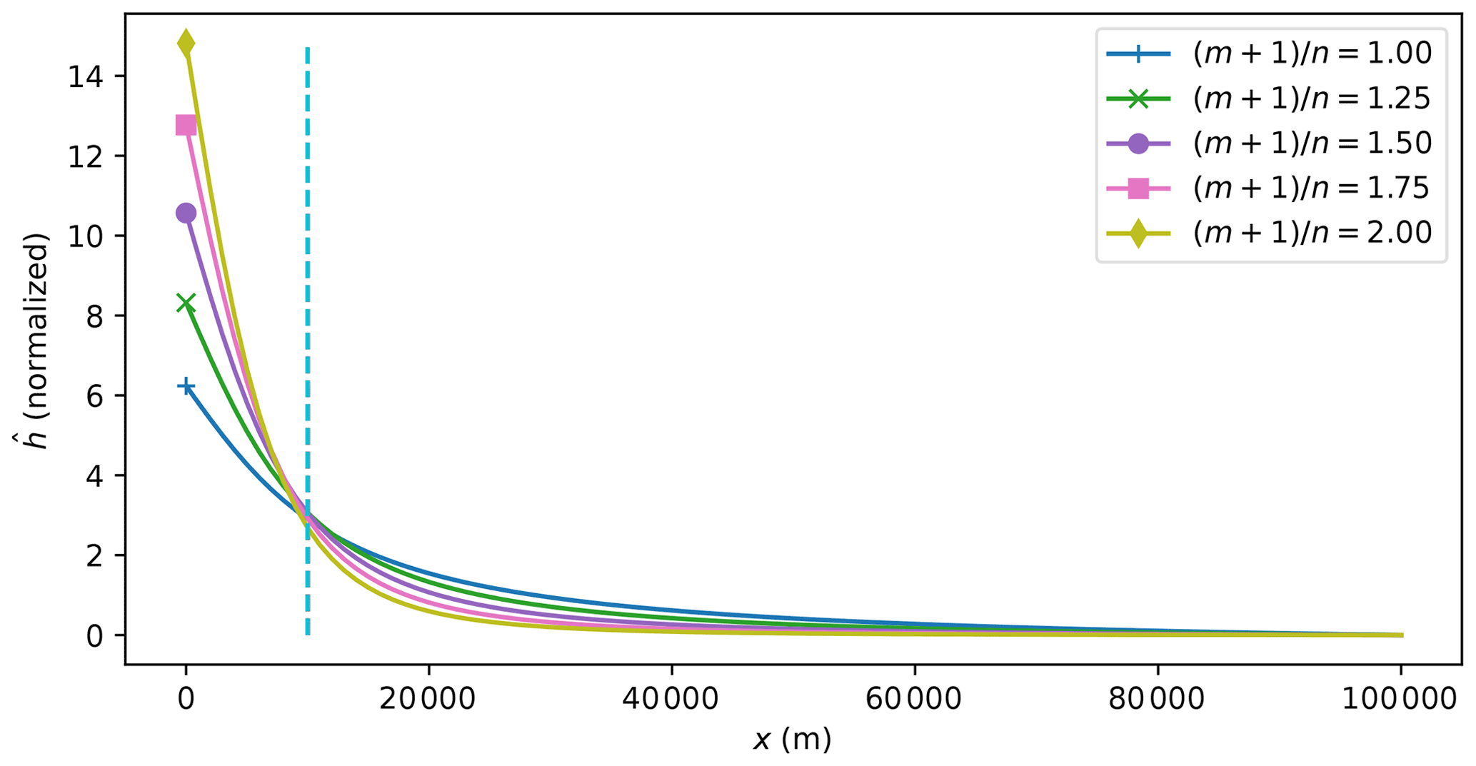
For open systems, the ratio controls the partitioning of the sediment flux between the fan and the alluvial plain. It also controls the difference in slope between the fan and the alluvial plain. For large values of , the fan is much steeper than the alluvial plain and traps a greater proportion of the sediment, for small values of , the fan slope tends towards the alluvial plain slope and a greater proportion of the sediment is deposited in the alluvial plain, as shown in Fig. 4.
3.2 Transient behavior
I now use the numerical algorithms described in the appendices to investigate the transient behavior of the solution. I first tested that the numerical models yield the steady-state analytical solutions. The results are shown in Fig. 3 where the numerical solutions have been superimposed on the analytical solution.
The transient behavior of the solutions to the two equations is shown in Fig. 5 for the three situations where (constrained systems, Fig. 5a), L=L0 (Fig. 5b) and (open systems, Fig. 5c). In Fig. 5, time has been normalized by the e-folding timescale, τ, determined by fitting each time–elevation curve by an exponential function of the form , while height has been normalized by the maximum height reached at the end of the numerical experiment. We see that the time evolution of the solution to the TL equation is always supra-exponential (i.e., it increases faster than an exponential) but that its shape is independent of whether the system is constrained or open. On the contrary, the shape of the time evolution of the solution to the ξ–q equation is dependent on , with a more gradual (linear) increase with time for constrained systems and a sub-exponential form for open systems.
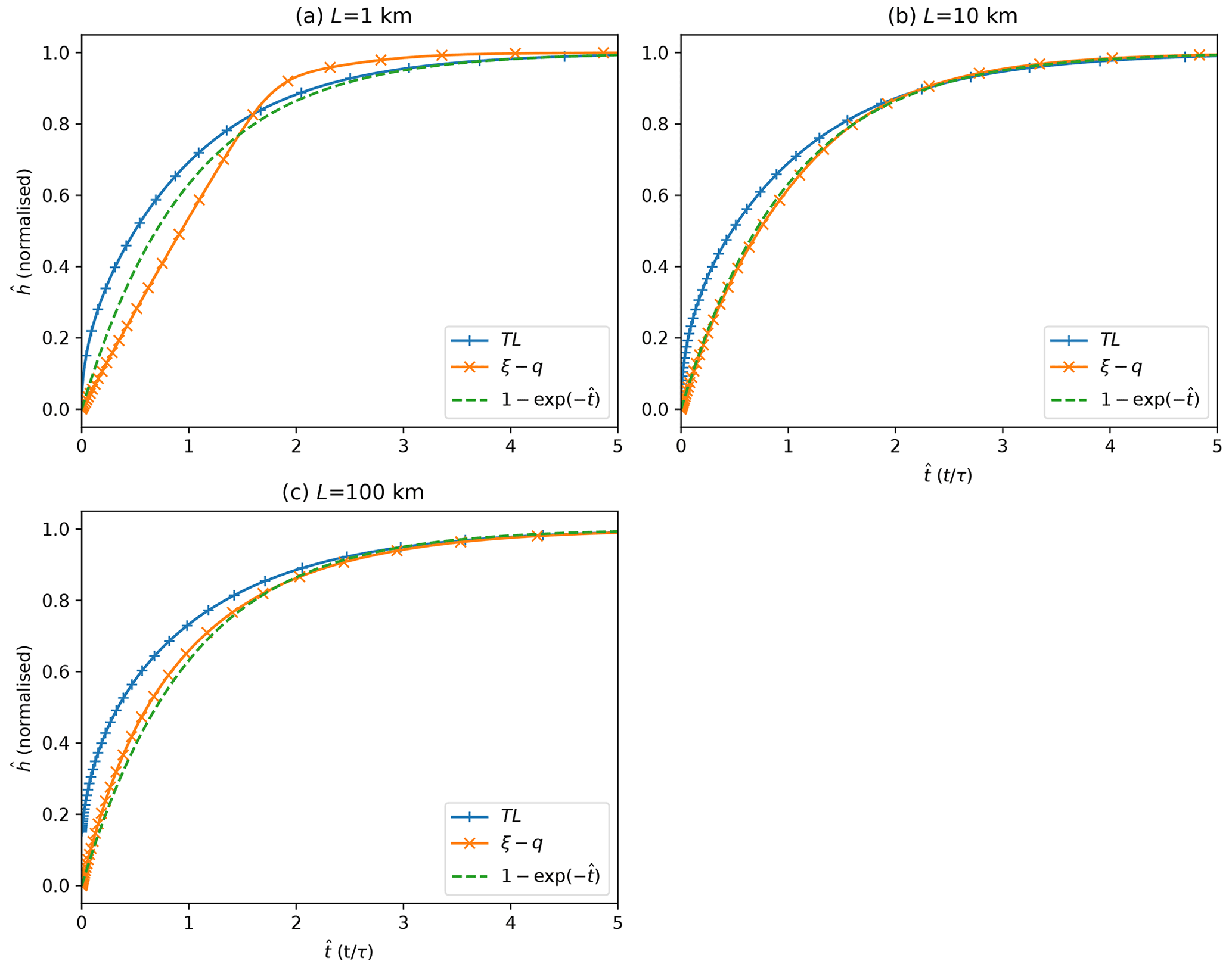
Figure 5Maximum surface elevation as a function of time. Surface elevation is normalized by its maximum value and time by the e-folding timescale, τ. The three panels correspond to different length of the system compared to L0 (a) (constrained systems), (b) L=L0 and (c) L=10L0. (open systems) In each panel the curves correspond to the solutions to the ξ–q and TL equations and are compared to the third curve representing an exponential increase of the form .
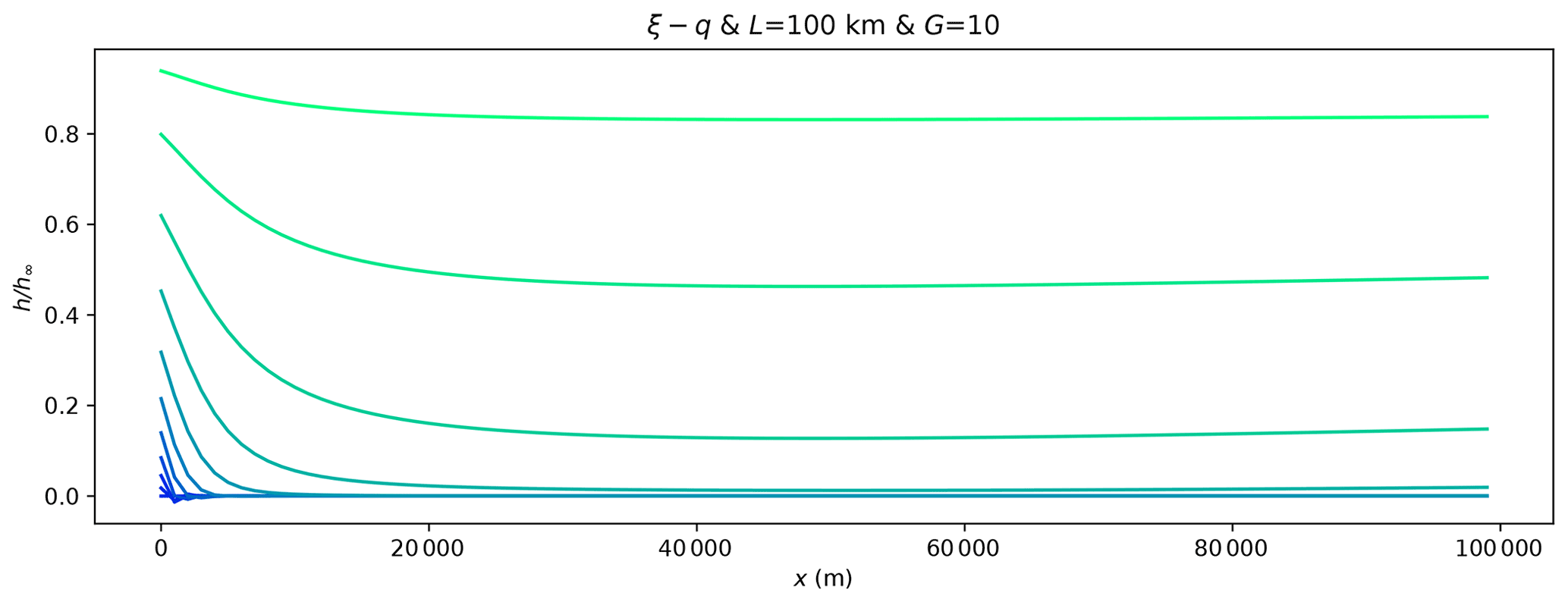
To further investigate the transient behavior of the two equations, I show the evolution of the predicted surface elevation of the system in Fig. 6. I show the same information in Fig. 7 but after scaling the computed height by the steady-state height (h∞) such that one can appreciate the behavior of the solution equally well along the entire profile, even when deposited thicknesses are very low. One sees a major difference between the two equations' behavior. The solution to the TL equation evolves by depositing sediments near the fan apex first until sediments reach the system toe (base level) at which point the solution evolves with a uniform (relative) rate of filling all along its length. The ξ–q equation yields a solution that evolves in the other direction, i.e., from toe to apex, as the sediment fill progresses first towards its steady-state solution near the toe of the system and then propagates backwards to reach a situation where the relative rate of filling is more uniform over the entire system. This difference in behavior is most striking for constrained systems (i.e., where L<L0), but exists for all system lengths, both constrained or open.

Figure 6Surface elevation at a series of logarithmically spaced time steps obtained by solving the ξ–q and TL equation for different system length, L, smaller than, equal to or greater than L0=10 km. Blue to green colors correspond to early to late time steps.
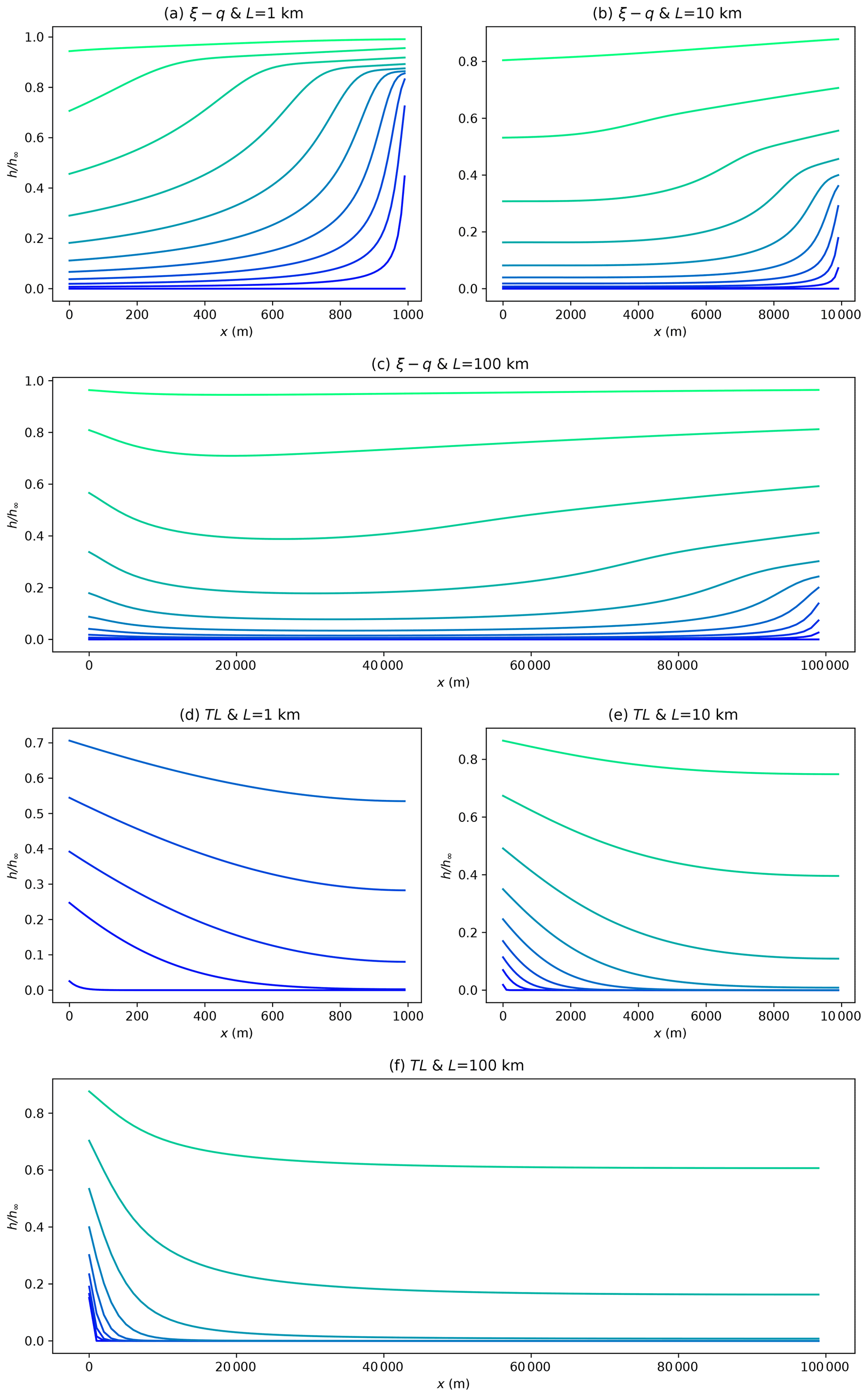
Figure 7The same information as in Fig. 6 but using the relative surface topography, i.e., scaled by its steady-state value.
This difference in topographic evolution is accompanied by major differences in the predicted flux out of the system (i.e., at x=L) during the transient phase of fan and alluvial plain build up as illustrated in Fig. 8 (expressions used to compute the flux values are given in Appendix D). In the ξ–q model, the flux out of the system is instantly finite, i.e., as soon as the sedimentary system starts to grow. In the TL model, the initial flux out of the system is always nil and remains so until the propagation of the sedimentary wedge reaches the toe of the system. In other words, the ξ–q model predicts an instantaneous flux response, regardless of the size or character of the system, whereas the TL model predicts a lagged response, with a phase shift that appears proportional to the length of the system. At all times (scaled by the response time of the system), the outgoing flux predicted by the ξ–q model is much greater than that predicted by the TL mode. This implies that the ξ–q solution is always much more “leaky” than the TL solution, as it requires a much greater amount of material to transit through the system before it reaches steady-state.
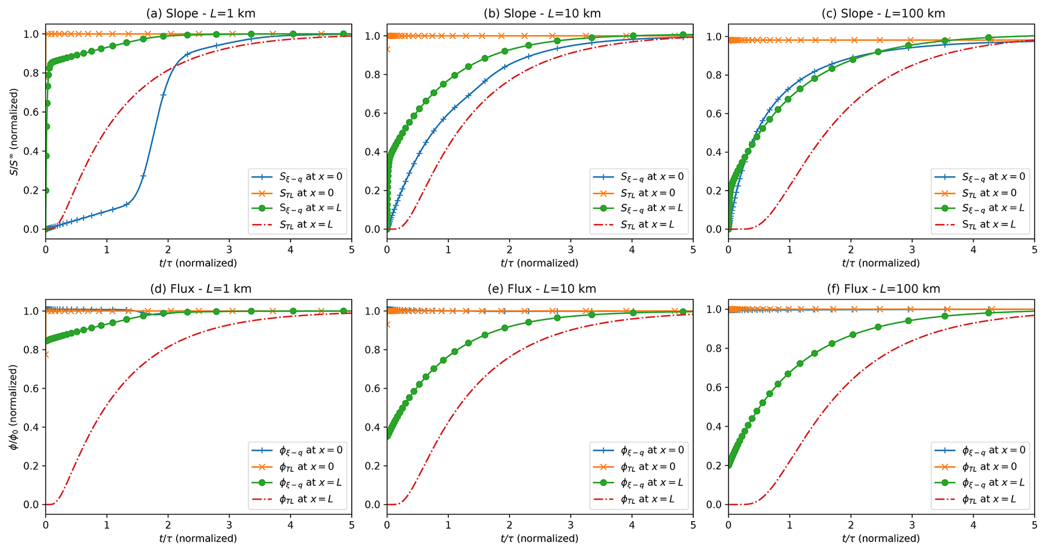
Figure 8Evolution of the slope (a–c) and flux (d–f) normalized by their steady-state values at both ends of the system as a function of time.
3.3 Response to a step change in incoming sedimentary flux and precipitation rate
I performed a series of experiments in which I abruptly changed the incoming sedimentary flux, q0, or the relative precipitation rate, ν. The results are shown for an increase in sediment flux in Fig. 9, and in the Supplement for a decrease in sediment flux (Fig. S1), for an increase in relative precipitation rate (Fig. S2) and for a decrease in relative precipitation rate (Fig. S3, for both models).

Figure 9Evolution of the surface topography following an increase in incoming sediment flux by a factor of 2. The ξ–q solution is used in the top six panels, and the TL solution is used in the bottom six panels. Panels (d) to (f) contain the same information as panels (a) to (c) but using the topographic elevation normalized by its final, steady-state value. The same applies for panels (j) to (l) with respect to panels (g) to (i).
We see that for an increase in sedimentary flux (Fig. 9), the system moves back towards a new steady-state profile first near the toe of the system for the ξ–q equation and first near the apex of the fan for the TL equation. The solution then evolves from toe to apex for the ξ–q model and from apex to toe for the TL model. So, even though the two solutions start at and tend towards the same steady-state solution, they differ in the way they evolve from one to the other and this is especially true for the constrained fan systems.
3.4 Response time
I have shown that an e-folding timescale, τ, can be derived from the shape of the evolution equation of the maximum surface elevation of the sedimentary system. This timescale is called the response time of the system as it corresponds to the time it takes for the system to reach its steady-state shape but also more generally the time it takes for the system shape to respond to change in its external forcings (incoming sediment flux or precipitation rate).
In Fig. 10, I show the results of 24 numerical experiments in which I solved the TL and ξ–q equations varying the value of L. For each experiment, I computed the response time by fitting an exponential curve of the type to the computed evolution of maximum elevation with time (upper panels in Fig. 10). The ξ–q response times are reported in Fig. 10c and the TL response time are reported in Fig. 10d as 24 circles. We see that for constrained systems (L<L0), the TL response time varies quadratically with L, whereas the ξ–q response time varies linearly with L. However, this dependence changes dramatically for open systems, i.e., when L becomes greater than the size of the orogenic system, L0. This threshold is marked by a star in both panels of Fig. 10. For intermediate size systems, i.e., when , there is almost no dependence of either response times on L. For large open systems, i.e., when L≫L0, the ξ–q response time varies as L1−mp while the TL response time varies as and can thus decrease as system size increases.
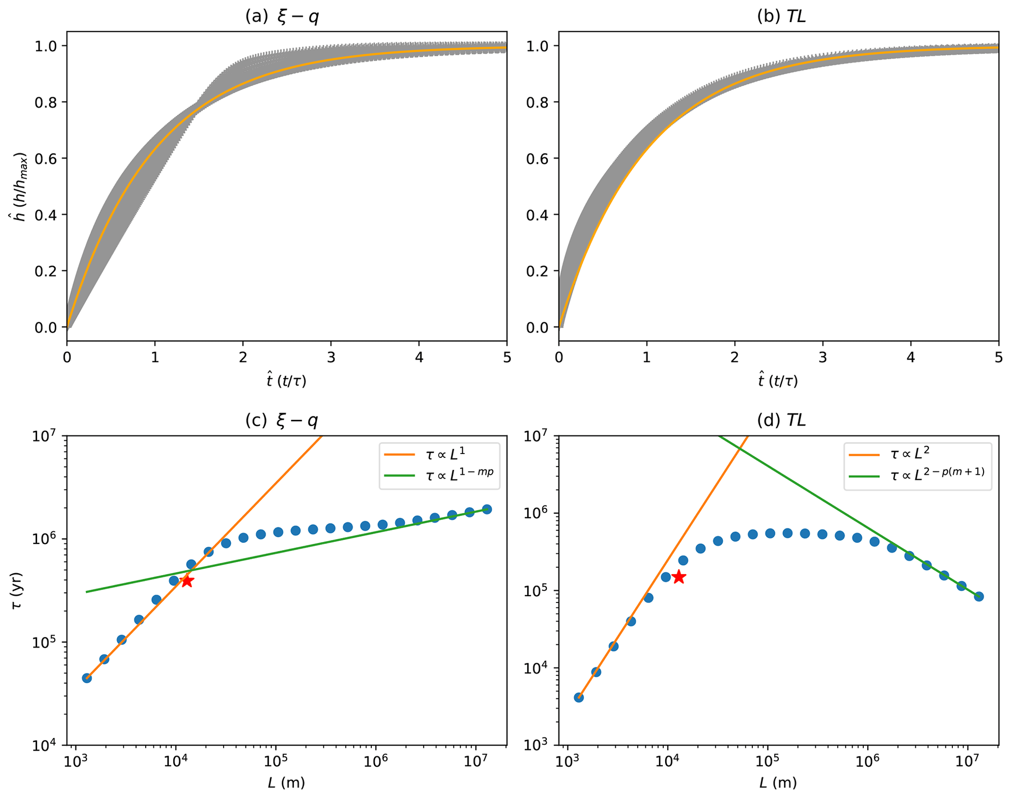
Figure 10Computed response times for 24 numerical experiments in which the length of the model, L, was varied. (a, b) Time evolution of the maximum height of the depositional system for all 24 experiments (grey curves) normalized to fit an exponential curve (orange curve). (c, d) Corresponding response time estimates (blue circles) on which lines describing the asymptotic behaviors discussed in the text have been superimposed. Note that the absolute values of the response times should be considered with caution as they correspond to a specific choice of relatively poorly constrained values of the rate parameters, Kf and Kd.
To understand this behavior, let us go back to Eqs. (3) and (7) to derive scaling relationships for the TL and ξ–q response times, τTL and τξ–q, respectively, for arbitrary values of m and n. For the TL equation, the scaling gives
From the steady-state solution (Eq. 15), we know that
which gives
For the ξ–q equation, the scaling is as follows:
with
Two cases must be considered, depending on the value of the dimensionless number:
If the equation is dominated by the erosional term (δ<1), the scaling is as follows:
whereas if the equation is dominated by the depositional term (δ>1), the scaling goes is follows:
regardless of the value of L with respect to L0, which is the same scaling as that of the TL equation for L<L0 and n=1.
Interestingly, δ is a nonlinear function of L that reaches a maximum value of
for . For p=2, δ is maximum for L=L0.
We see that for constrained systems, the TL response timescale follows the n+1st power of length but that for open systems this scaling is inverted, i.e., the TL response time decreases with length, almost regardless of the value of n. For constrained systems, the ξ–q response timescale scales at most with the length of the system, but for open systems the scaling drops to a small power. Again this behavior is relatively independent of the linearity of the system.
Both response times are independent of the incoming flux, q0, in linear systems and decrease with a small power of q0 in nonlinear systems. Both timescales vary inversely with the rate constants (diffusivity or erodibility), and in the linear case the ξ–q response time is independent of G in erosion-dominated systems and increases linearly with G in deposition-dominated systems.
In Appendix B, I show how the response timescales vary with the various characteristics of the systems for a range of values of the exponents m and n.
In Appendix C, I present the results of several series of numerical experiments, demonstrating the validity of the scaling I present above.
3.5 Comparison of response timescales
We have seen that the two equations lead to an identical steady-state solution when the model parameters are judiciously chosen to be in the ratio GKd=Kf. For their transient behavior to be similar requires (at a minimum) that their response times be also similar. This implies for constrained systems that
and for open systems that
For the solution to the two equations to have the same transient behavior, regardless of the length of the system, we must have
It is therefore impossible for both equations to reproduce the transient behavior of constrained and open systems with a unique set of parameters. Only the particular case of L=L0 is an exception to this.
Considering now a system of arbitrary length L, the ratio of the two timescales is
showing that for values of G close to unity and for a choice of model parameters that lead to the same steady-state solution, the ξ–q model will generate longer timescales than the TL model in a ratio equal to the ratio of the total upstream drainage area to the area of the floodplain (the part of the drainage area where active sedimentation or erosion and transport takes place).
3.6 Periodic variations in input flux
I now investigate how the system reacts to a periodic perturbation in incoming sedimentary flux from the source or orogenic area. I will consider first how the system shape reacts and then how it transmits the sedimentary flux signal from the source (the orogenic system boundary) to the sink (the base level boundary).
In Fig. 11a and b, I show the gain, Γh, and phase shift, ϕh, of the response of the system measured as the variation of the maximum topography, i.e., at the orogenic front of the sedimentary system, as a function of the forcing period normalized by the response time. The gain is the ratio of the relative amplitude of the response (i.e., the amplitude of the variations in maximum height scaled by the maximum height at steady state) to the relative amplitude of the forcing (i.e., the amplitude of the incoming flux variations scaled by the mean incoming flux). The phase shift is measured between the response and the forcing normalized by the forcing period. A phase shift of 0.25 corresponds to an angular phase shift of 90∘.
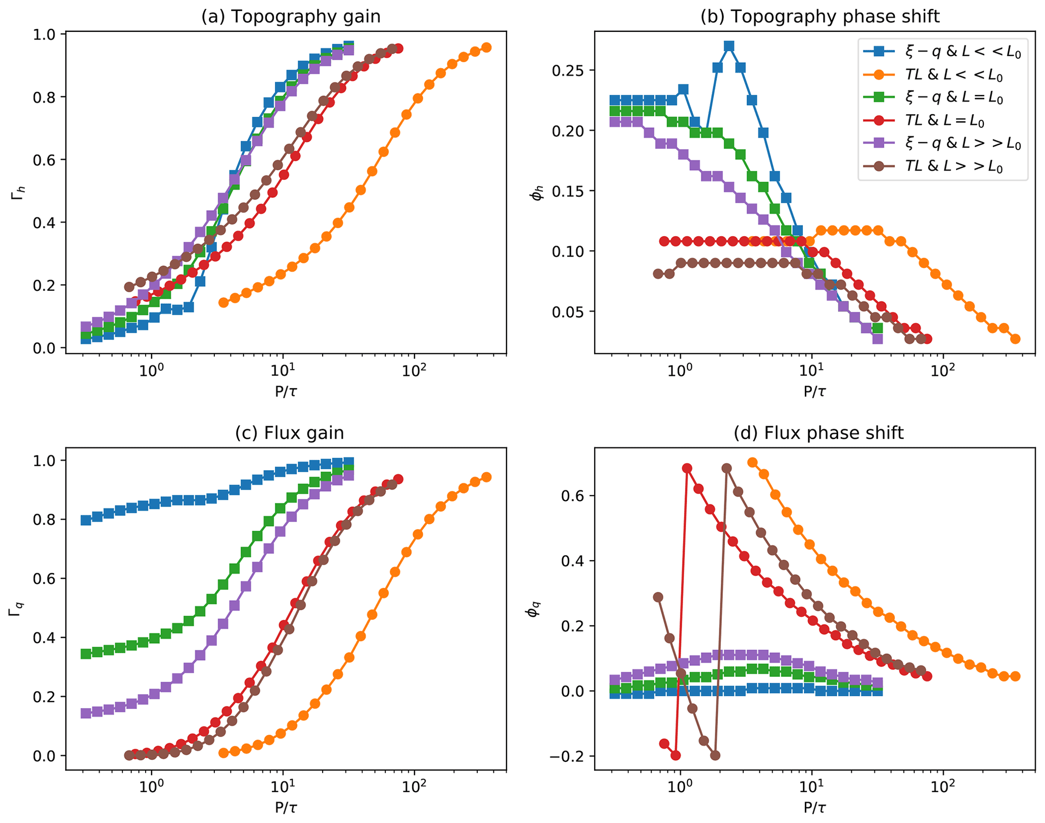
Figure 11Computed (a) gain, Γh, and (b) phase shift, ϕh, of the response of the system shape as a function of the period of the imposed periodic incoming flux normalized by the system's response time for constrained (L<L0), intermediary (L=L0), and open (L>L0) systems using the ξ–q and TL models. Computed (c) gain, Γq, and (d) phase shift, ϕq, of the outgoing sedimentary flux.
We see that for both models, the gain decreases from 1 to 0 as the forcing period decreases. For rapid (or short) forcing periods, i.e., much smaller than the response time, the gain tends towards 0, while for slow (or long) forcing periods, the gain tends towards 1. In other words, the system shape is less affected by variations in incoming flux that are smaller (or faster) than the characteristic timescale, regardless of whether the system is constrained or open, while variations in sedimentary flux are more strongly expressed as variations in deposited sediment thickness when the variations in incoming flux are longer than the characteristic timescales, regardless of whether the system is constrained or open.
We also see that the phase shift is a strong function of the forcing period: for large forcing periods, the phase shift tends toward 0, while for forcing periods that are equal to or smaller than the characteristic timescale, it grows to reach values of about 0.125 for the TL model and 0.25 for the ξ–q model, regardless of whether the system is constrained or open.
In summary, variations in system topography will be recorded in the sedimentary record as variations in deposited (and eroded) sediment thickness. These will be largest near the orogenic front but will be noticed at all locations within the sedimentary system. At most (i.e., when Γh=1) their amplitude will be directly proportional to the amplitude of the flux variations. When the system most strongly reacts to the variations in incoming flux (i.e., when Γh≈1), it does it in phase with the forcing (ϕ≈0); phase shifts only appear when the response is weak. This means that if a system is responding in a noticeable manner to a change in incoming sedimentary flux, it does it with a minimal phase shift.
In Fig. 11c and d, I show the gain, Γq, and the phase shift, ϕq, between the incoming and outgoing fluxes. These quantities characterize the ability of the system to transmit sedimentary flux signals across their length.
Interestingly, the gain functions are radically different for the ξ–q and the TL models. Regardless of whether the system is constrained or open, the TL model predicts that the gain varies from 1 to 0 as the forcing period decreases from values larger than the characteristic timescales to values smaller than the characteristic timescales. The TL model predicts that a sedimentary system can only propagate signals that vary more slowly than their characteristic timescales. Note also that as the signal is damped (with decreasing forcing period) the phase shift increases to become more than a quarter cycle out of phase (ϕq>0.25) with the input signal. This is because the TL model predicts that incoming flux variations propagate as standing waves across the sedimentary system.
This is illustrated in Fig. 12, where I show the computed sedimentary flux across the entire system for 10 equally spaced time steps within a forcing period (see Appendix D for the expressions used to compute the fluxes for both models). We see for the TL model that the slow signals are transmitted through the entire system, whereas rapid signals are not. In the situation where the forcing period is similar to the characteristic response time (in Fig. 12g), one sees a standing wave pattern developing across the system. This is because in the TL model, any signal must be transmitted by changes in slope, and such a change can only occur over a time equal to the characteristic timescale.
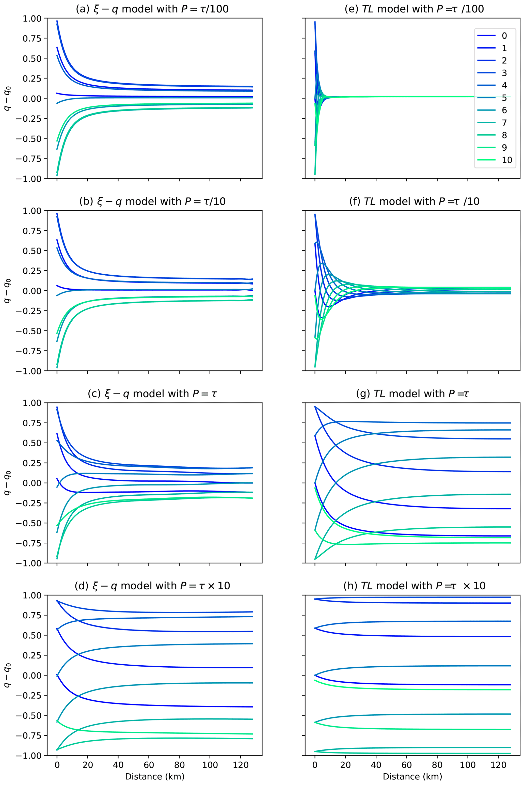
Figure 12Computed flux profiles across the sedimentary system at 10 time steps within one of the imposed incoming flux cycles (a–d) using the ξ–q model and (e–h) using the TL model. Going from top to bottom, the forcing period is equal to , , τ, and 10×τ, respectively. In all cases shown, L=10L0.
In contrast, we see in Figs.11c, d and 12 that using the ξ–q model the sedimentary system is predicted to transmit information along its entire length without much change in slope or shape. As stated by Davy and Lague (2009), and contrary to previous under-capacity formulations such as that of Kooi and Beaumont (1994), the ξ–q model predicts that the system is uniformly under-capacity along its entire length. It does not display a transition from being a detachment-limited model near the source to being a transport-limited model near the base level. Thus, it is able to transmit signals nearly instantaneously and with much less sensitivity to the forcing period. This is seen in Fig. 11c where the flux gain function never reaches 0 even for very rapid forcing periods. This is further illustrated in Fig. 12a to d, where the incoming flux variations are transmitted throughout the entire length of the system even if the forcing period is much shorter than the characteristic time of the system (Fig. 12a).
3.7 Periodic variations in precipitation rate
I performed a series of numerical experiments in which I varied the precipitation rate, ν, in a sinusoidal fashion, for a range of periods encompassing the response time of the sedimentary system. The results are shown in Fig. 13 and are relatively similar for the ξ–q and TL models.
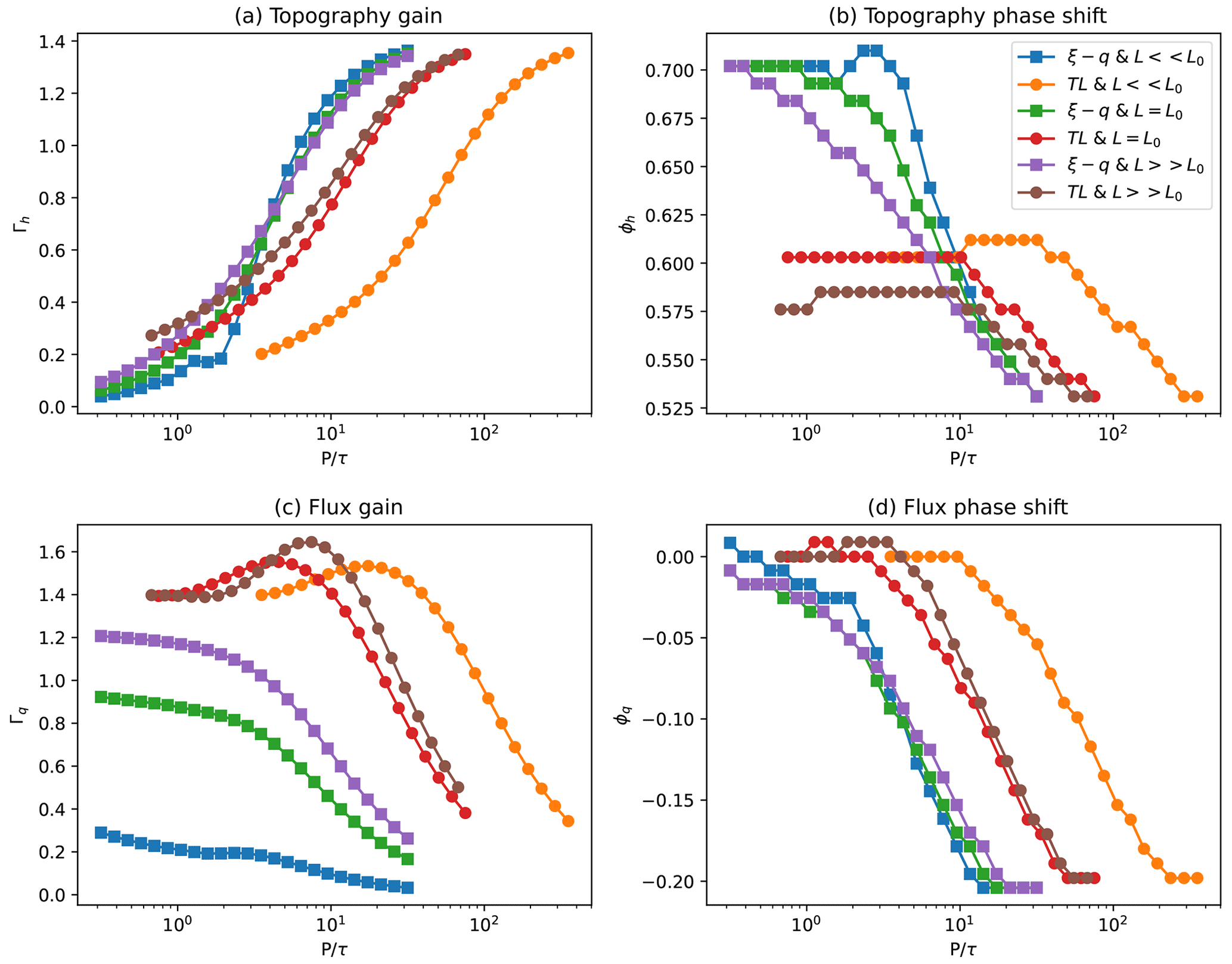
Figure 13Computed (a) gain and (b) phase shift of the response of the system shape as a function of the period of the imposed periodic precipitation rate normalized by the system's response time for constrained (L<L0), intermediary (L=L0), and open (L>L0) systems using the ξ–q and TL models. Computed (c) gain and (d) phase shift of the outgoing sedimentary flux.
These experiments show that variations in precipitation rate cause variations in deposited thickness in the sedimentary system that vary in amplitude as a function of the forcing period, similarly to variations in shape/thickness predicted for a incoming sedimentary flux forcing: for forcing periods that are smaller than the response time of the system, the amplitude tends towards zero and increases with the length of the forcing period. However, predicted gain values for very long forcing periods (>10 to 100×τ) tend towards 1.6>1. This is because the relative precipitation rate comes to the power in the amplitude of the analytical solutions (Eqs. 15 and 16).
Another major difference is that the shape response is in complete phase opposition (ϕ=0.5) for the largest gain values (corresponding to long forcing periods) and increases to even greater phase shift values for forcing periods smaller than the response time. This is because the relative precipitation rate appears in the denominator of the amplitude of the analytical solutions; in other words, the thickness of the sedimentary deposit is inversely proportional to the relative precipitation rate (to the power m+1).
The outgoing flux gain and phase shift are shown in Fig. 13c and d. Interestingly, the gain values decrease with increasing periods. This is because for precipitation rate forcing periods that are larger than the characteristic timescale, the depositional system is able to adapt its shape to transport the incoming flux at all times, regardless of its transport capacity (determined by the precipitation rate). As for the topographic gain, values can be larger than one (up to ). The phase shift is nil for large values of the gain and reaches a quarter period for small values of the gain (corresponding to long periods).
In Fig. 14 I further illustrate this point by showing values of the flux across the entire system at 10 different times during one of the precipitation rate cycles. The pattern is inverted compared to that observed for a cyclic forcing in incoming sedimentary flux (i.e., compared to results shown in Fig. 12): fast varying perturbations are transmitted or even amplified, whereas slow varying perturbations are completely damped for both the ξ–q and TL models.
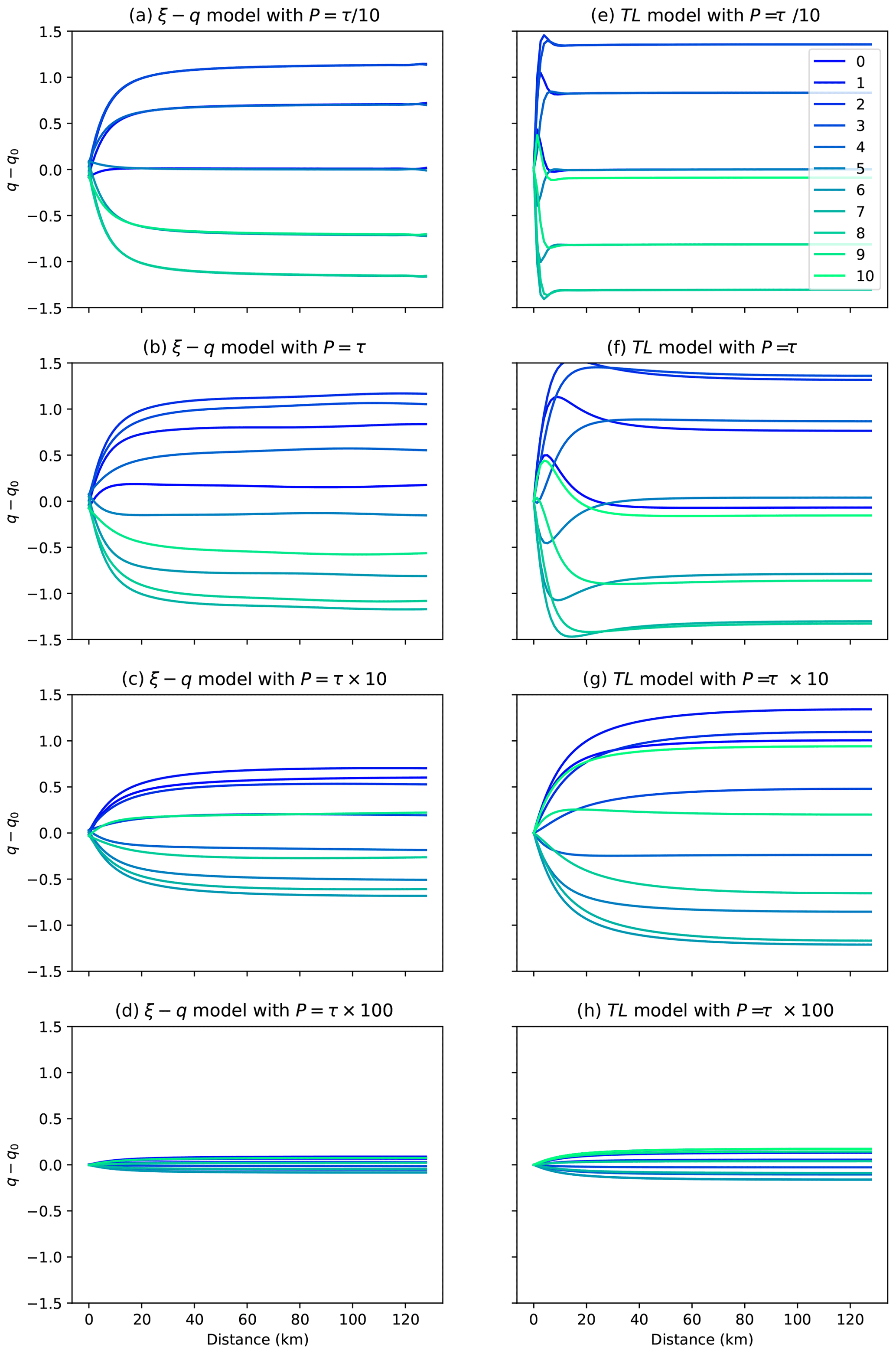
Figure 14Computed flux profiles across the sedimentary system at 10 time steps within one of the imposed precipitation rate cycle (a–d) using the ξ–q model and (e–h) using the TL model. Going from top to bottom, the forcing period is equal to , τ, 10τ and 100×τ, respectively. In all cases shown, L=10L0.
4.1 New analytical solution
I have derived a new analytical solution for the shape of a sedimentary system comprising a fan or piedmont deposit and the adjacent alluvial plain. This analytical solution shows that both model formulations can reproduce these first-order features and that in both models the transition between fan and plain deposits corresponds to the point where the contribution to runoff from the sedimentary system equals that of the upstream orogenic area. The fan is steeper and more linear, and its size is controlled by the size of the upstream catchment and the along-stream rate of increase of discharge in the sedimentary system (the exponent of the assumed Hack's law). The alluvial plain is characterized by a smaller gradient and has a concave profile. The analytical solution also implies that the change in surface gradient between the fan and the plain is a strong function of the ratio , which must be of the order of unity to reproduce the observed range of 10:1, with fan slopes ranging from 1 to 10∘, while adjacent alluvial plain have slopes that are typically smaller than 0.5∘ (Bowman, 2019).
This new analytical solution explains the globally observed linear relationship between fan area, Afan and upstream or orogenic drainage area, A0 (Fig. 14.23 in Blair and McPherson, 2009, for example) as
and the inverse relationship (with a log–log slope of −0.5) between the slope of the fan, Sfan, and the upstream drainage area (see Fig. 9 in Mouchené et al., 2017, for example) as
It also explains the relationship between fan slope and sediment flux scaled by upstream water discharge observed in experimental settings (Whipple et al., 1998) as
Experimental work suggests that the break in slope at the foot of a sedimentary fan is a result of grain size control on transport efficiency (Parker et al., 1998). Interestingly, I show here that the break in slope can be produced with a model that does not include a grain size control on transport coefficient (Kd) or depositional parameter (G). Because the model produces the observed area and slope scalings with upstream catchment area (something that cannot be derived from the grain size dependence on transport efficiency alone), I would like to suggest that the observed transition in grain size at the foot of sedimentary fans may be a consequence of the change in transport efficiency rather than the cause of it. But this remains to be tested, potentially by performing experiments that consider rainfall accumulation and the contribution to discharge within the sedimentary system.
As observed in nature, the analytical solution also shows why sedimentary systems are constrained in their size and shape by the location of or distance to their base level (Blair and McPherson, 2009). If that distance is small, such as in situations where a large river, a lake or an ocean is situated in the vicinity of the orogenic front, the fan is steep, almost perfectly linear and connects directly to the base level. This morphology is observed in many small systems, such as the Death Valley fans (Bull, 1977; Blair and McPherson, 2009). On the contrary, if that distance is large, the system is open and the fan can develop into its natural size and connects to a lower gradient alluvial plain where a concave-up long profile develops to connect the fan to the base level. I wish to stress here that the qualifiers “small” and “large” do not refer to the absolute size of the system but must be considered in comparison to the size of the upstream catchment area.
Finally, the analytical solution also demonstrates that the shape and size of a fan can reach steady-state values even if the fan does not extend to its base level and can therefore be seen as a simple solution to the so-called “alluvial fan problem” described by Lecce (1990), i.e., whether fans achieve a dynamic equilibrium. This solution also demonstrates why this debate about whether fans reach steady-state sizes or shapes could not be resolved by laboratory-scale experiments as most do not include a contribution to runoff from the depositional area.
4.2 What do the two models have in common?
The ξ–q and TL models share their steady-state solution. With an appropriate choice of rate parameters, i.e., Kd and Kf, and dimensionless constant G, the two solutions can be made identical. Acknowledging that we do not know the value of either of these three parameters leads to the conclusion that the two models cannot, in practical terms, be differentiated based on the shape of their long-term, steady-state solution. As noted above, both models can reproduce the first-order features of natural sedimentary systems, which implies that they should not be discriminated on that basis.
Both models share a similar behavior under a wide range of situations in that their transient response is (in all cases) controlled by the ratio of the period of the forcing to their response timescale. This is however true of most systems controlled by diffusion- or advection-type differential equations and is therefore not surprising.
In particular, regardless of which model is used, only slow incoming sedimentary flux variations (i.e., with a period greater than the response time of the system) will result in variations in deposited or eroded sediment thickness in the sedimentary system that are more likely to be measured, whereas only fast variations in precipitation rate will result in easily measurable variations in sediment thickness.
4.3 Where do the two models differ?
The ξ–q and TL models differ in their transient behavior in three ways. Firstly, they differ by the value of their response time with the ξ–q model characterized by longer response times than the TL model under the assumption that model parameters are such that the two models predict the same steady-state solution. The ratio of the ξ–q to TL model response times is a function of the ratio of the area under active sedimentation, transport or erosion and the drainage area. The reason for greater response times for the ξ–q model is that the model predicts a transient response that is uniformly distributed along its length, whereas the TL model responds by progressively changing its surface slope across the model. This implies that the ξ–q model predicts that any perturbation is instantaneously propagated to the system base level and affects the outgoing flux through base level making the system more “leaky” than the TL model. One can show (see Appendix E) that the TL response time for a constrained fan system (i.e., where L≪L0) is approximately equal to twice the volume of the fan divided by the incoming flux, which indicates that during the transient build-up of the fan, most of the material introduced into the fan from the orogenic area has been stored into the fan. The ξ–q response time is greater by a factor .
Secondly, they differ in the dependence of their response timescale on the length of the system and, to a lesser degree, on the size of the upstream area and the width of the floodplain. Constrained systems (or systems that are not able to develop a plain in front of their fan) have a response time that varies as the square of the length of the system in the TL model and as the length of the system only in the ξ–q model. Both models predict a response time that shows a very weak dependence on the length of the system for intermediate-sized systems (L≤L0), but for very long systems (L≫L0) the TL model response time varies inversely with the length of the system (the longer the system, the shorter the timescale), whereas the ξ–q model response time increases with the system length.
Thirdly, the models differ in the way that they are able to transmit sedimentary signals. According to the TL model, only slow perturbations in incoming sedimentary flux will be transmitted through the system and may therefore be recorded in the adjacent basin. If one uses the ξ–q model to represent a sedimentary system, all flux perturbations will be transmitted to the offshore basin, regardless of the rate at which they take place. The higher-frequency signals will be slightly damped compared to the low-frequency signals, but all of them are transmitted in a potentially measurable manner.
4.4 Are the differences meaningful?
An important question to address is whether these differences are relevant and/or important and in which context. Considering that both models are reduced-complexity models that should only be used to investigate the large-scale and long-term behavior of a sedimentary system, I suggest that great care should be taken in deciding which of the two models to use to investigate the transient behavior of sedimentary systems and their response to external forcing of tectonic or climatic origin in particular. This is particularly true in so-called source-to-sink studies that aim to invert the marine sedimentary record to infer the timing and amplitude of tectonic or climatic changes in the source area. I have shown that the so-called “transfer area” that consists of the onshore sedimentary system that builds up at the base of the mountain (the fan and the adjacent alluvial plain) would appear to have very different transient behaviors whether one uses the ξ–q or TL model to represent it. Most worrying is the fact that according to the TL model some sedimentary signals cannot be transmitted across the transfer zone, while the ξ–q model does not predict such a behavior. More fundamentally, that the response timescales predicted by the two models are different and show a different scaling and dependence with regard to system length should also be noted and could lead to diametrically opposite conclusions regarding the existence and/or nature of orogenic processes and their preservation in sedimentary systems.
4.5 What observations could be used to tell the models apart?
To differentiate between the two models or representations of sedimentary processes, one obviously needs to search into observational constraints during transient periods either in the early stages of development of a sedimentary system or during its response to external perturbations. The first type of observations are not easily made as the early stages of development of a fan are often buried beneath large sedimentary sections. The second type of observations require accurate dating or correlation across opposite parts of the sedimentary system, i.e., near the orogenic front and either at the base of the fan or near the base level of the sedimentary system.
Another test comes from the prediction that according to the ξ–q model some signals should propagate and be stored into a nearby sedimentary basin record even if they are shorter than the response time of the system, regardless of whether or not such signals leave a stratigraphic record in the continental sedimentary system. In view of the wide range of periods (down to the shortest of Milankovitch periods) that are routinely observed in the marine sedimentary record, one would tend to favor the ξ–q model over the TL model. However, one must exercise caution in drawing such a conclusion as such signals might be the product of variations in sea level rather than variations in sediment flux from the source or orogenic area.
The distribution of grain size in continental sedimentary systems has been used to constrain their transient behavior (Armitage et al., 2011; Duller et al., 2010), but most studies have been based on the approximation that deposition is equal to basin subsidence (Duller et al., 2010) or have used a nonlinear diffusion (TL) approach (Armitage et al., 2011). It would be potentially very informative to perform similar studies using the ξ–q model and note if noticeable differences emerge between the two approaches and whether they are of sufficient amplitude to be discerned in field observations.
Laboratory experiments could be used but one must remember that they only reflect the behavior of scaled-down materials and conditions and not the natural world. Furthermore, looking at the results of several published experiments tends to demonstrate that both behaviors are observed. In Fig. 15a–c, I show the results of three experiments under relatively similar conditions: the first and third ones from Guerit et al. (2014) and Rhohais et al. (2012) show a sedimentary fan developing by propagation of a self-similar system under constant slope, as predicted by the TL model (Fig. 6d), whereas the second one from Whipple et al. (1998) shows a response to varying conditions (flux) that resembles the predictions of the ξ–q model (Fig. 6a). Note, however, that none of these experiments take into account the discharge being contributed from rainfall or runoff in the sedimentary system, i.e., the discharge is set at the left boundary. Differences between the two experimental setups include the dimensionality (1D for the experiments of Guerit et al., 2014, and 2D for those of Rhohais et al., 2012 and Whipple et al., 1998) and the nature of the flow (laminar in the Guerit et al., 2014, experiments and turbulent in the other two).
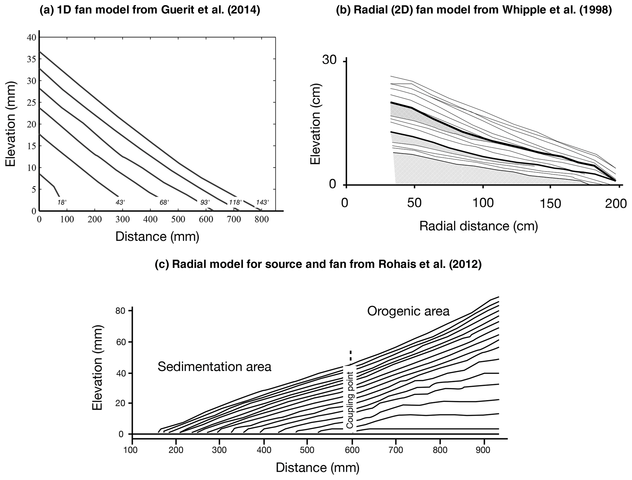
Figure 15Stratigraphy observed in three laboratory experiments displaying a behavior similar to that predicted by (a, c) the TL model (from Guerit et al., 2014; Rhohais et al., 2012) and (b) the ξ–q model (from Whipple et al., 1998). Note that none of these experiments included rainfall in the fan area. Panel (a) is reproduced from Guerit et al. (2014), (b) is from Whipple et al. (1998) and (c) is from Rhohais et al. (2012).
4.6 Value of G
All the experiments I have performed with the ξ–q model used a value of G=1. As shown by Guerit et al. (2019), observations from natural sedimentary systems suggest a range between 1 and 2 for G. It is also in this range that the ξ–q model shows the most interesting behavior. For values of G≫1, the model tends to behave exactly like the TL model with, for example, an identical dependence of the response time on system length and a geometrical evolution that is identical to that of the TL model as shown in Fig. 16. For values of G≪1, the ξ–q model predicts that the transfer system is very small, i.e., the volume of sediment that it can store is negligible. This would lead to fan slopes that are much lower than observed in nature.
4.7 Hack's law in a depositional system and optimum values of m and n
In setting up the experiments, I have assumed for both models that Hack's law applies to depositional systems. Edmonds et al. (2011) showed that even low-slope depositional environments such as deltas obey Hack's law with an exponent (p) very close to 2. We can also check that this holds using a 2D landscape evolution model that solves the ξ–q equation based on the algorithm developed by Yuan et al. (2019). The model geometry is of a sediment–water point source feeding material over a flat area of 100×100 km. Three experiments were performed assuming upstream drainage areas, A0, of 107, 108 and 109 m2, respectively. In Fig. 17 I show the geometry of the 10 longest channels originating from the center of the model where the sediment–water flux is imposed (Fig. 17a), as well as the relationship between distance to the source (center of the model) and drainage area (Fig. 17b). We see that in all three experiments, the most active channel has a distance–drainage area relationship that smoothly transitions from A0 to a relationship described by Hack's law with an exponent of 2. Most other channels that form along the sides of the fan and flow unto the edges of the model follow Hack's law with an exponent of 2.
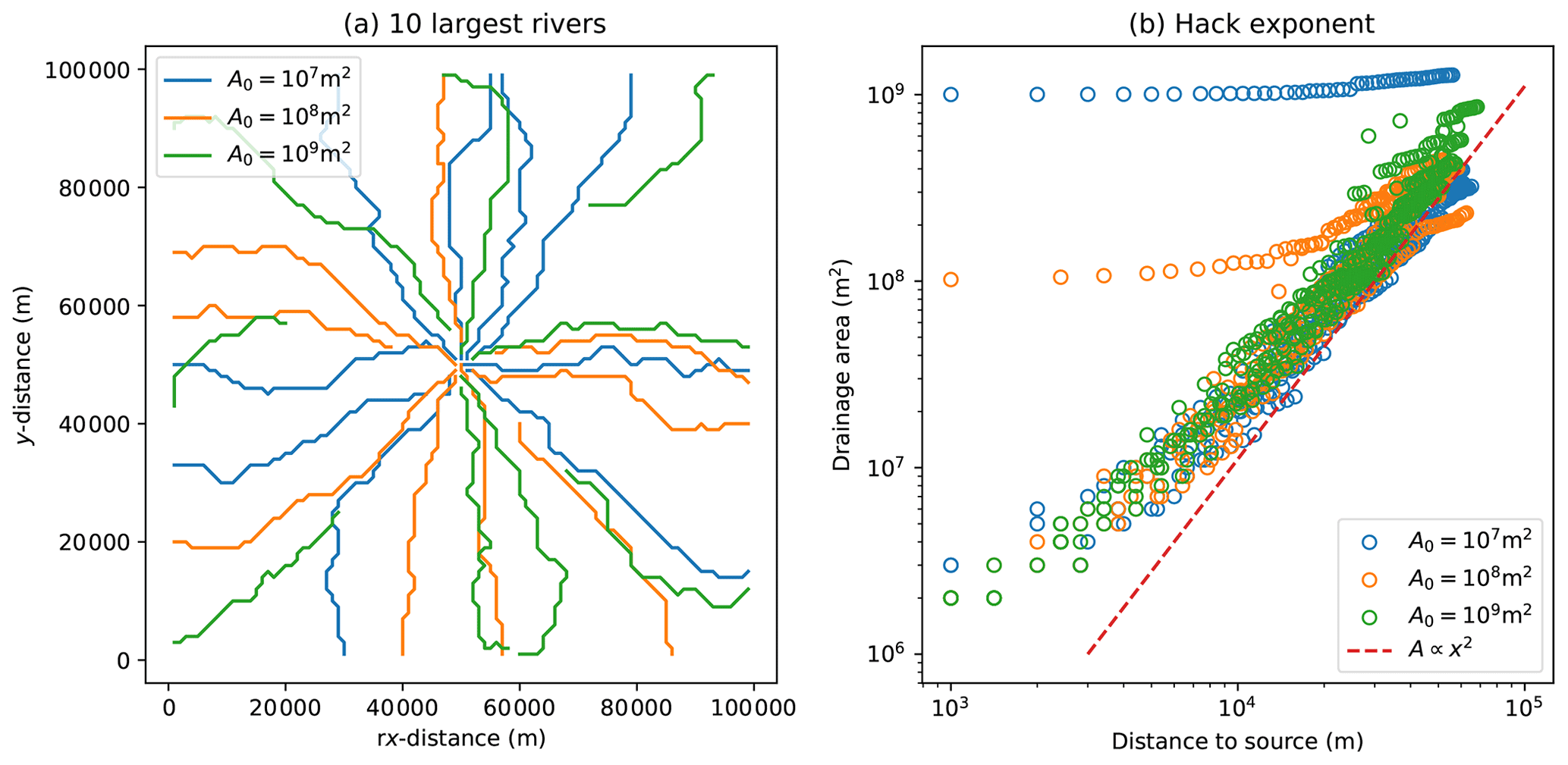
Figure 17Results of three two-dimensional landscape evolution models where sediment and water are provided at a rate proportional to the surface area, A0, of an assumed upstream catchment at the center of the model leading to the formation of a conic sedimentary system. The three models correspond to three different values of A0. (a) Geometry of the 10 major rivers for each of the three models and (b) computed relationship between drainage area and distance to source for those 10 major rivers; the dashed red line has a slope corresponding to an exponent of p=2 in Hack's law.
If this interpretation is correct, it implies that to reproduce the observed linear relationship between upstream drainage area and fan size, the value of p must be close to 2 even in the fan where the system by definition traverses the transition between confined and unconfined water flow. I have shown (Fig. 4) that the partitioning of sediment between the fan and the alluvial plain is determined by the value of the ratio . To obtain a significant break in slope between the fan and the alluvial plain, i.e., as is observed in many natural systems (Blair and McPherson, 2009), the ratio must be in the range [1 to 2] (see Fig. 4). This in turn implies that the most likely values of m and n are in the range [1 to ] and [2 to ], respectively, as the concavity of river channels implies that . Of course this is only valid if we wish to have a representation of both the orogenic and depositional parts of the system with a unique set of exponents, an objective that may only be realistic in the context of a reduced-complexity model that is designed to reproduce the long-term and system-scale features of the source-to-sink system and not the details of the physical processes at play.
To further illustrate this last point, I computed the effect of varying both Hack Law's parameters (k and p) on the shape of the steady-state solution. The results are shown in Fig. 18 and show that varying the rainfall rate (or changing the value of k) in the basin area (compared to the orogenic area) results in a wider fan for greater values of k and vice-versa. Changing p also affects the fan steepness. Lower p values (compared to 2) lead to a much reduced slope contrast between the fan and alluvial plain areas.

Figure 18Effect of varying Hack's Law (A=kxp) parameters (p in a and k in b) on the depositional system steady-state profile. The vertical dashed line represents the position of ). Because k has units that depend on p in (a), k has been adjusted to yield the same value of L0 for all values of p.

4.8 Residence time
Both equations used here to model sediment transport are expressed in an Eulerian framework, i.e., using a frame of reference that is fixed with respect to the system's boundaries. Such an approach does not easily permit tracking sediment particles and estimating their residence time inside the fan or alluvial plain system as done by Carretier et al. (2020). An alternative approach consists of approximating the residence time, τR, using the turnover time that is defined as the ratio between the volume of the active part of the transporting system, Va, and the imposed sediment flux, q0:
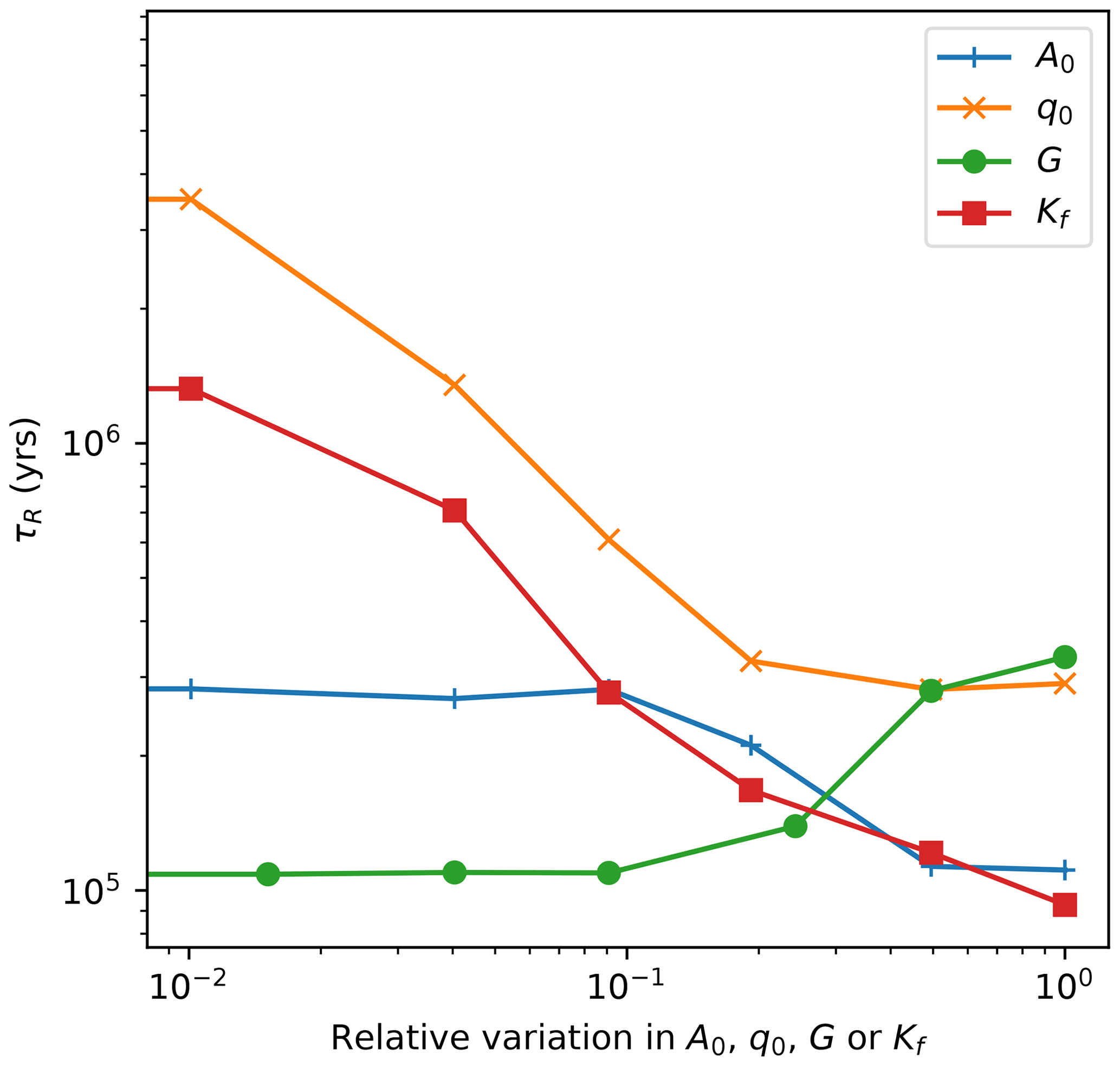
At steady state, Va is the integral over the sedimentary domain of the thickness of the active layer, ha(x,y), that can be approximated by the standard deviation of the surface topography over many time steps. This can only be computed using the 2D model where avulsions affect the upper layers of the model. I show in Fig. 19 computed values of this residence time as a function of the main model parameters, A0. q0, G and Kf for a 2D model setup similar to the one used in the previous section, i.e., for model parameters and sizes identical to those used for the model run shown in Fig. 17. We see that the residence time varies between 105 and 106 years. More importantly, the model predicts that the residence time varies as and over at least 1 order of magnitude variation in these parameters. It also increases quasi-linearly with G for values of and varies with the upstream catchment area as , as expected.
4.9 Effect of basin subsidence on fan size and shape
All results shown so far assume that there is no subsidence in the depositional area. However, most regions adjacent to a mountain belt (or sediment source) experience synorogenic subsidence likely driven by flexural isostasy. It has been suggested that the pattern of this subsidence exerts a strong influence on the shape of the resulting alluvial fan (Paola et al., 1992; Parker et al., 1998). I tested the influence of basin subsidence on the shape of the depositional system by running numerical experiments similar to the reference model presented in Fig. 3 but adding a subsidence term of the following form to both Eqs. (3) and (7):
where s0 is the maximum subsidence rate at the mountain front and α controls the rate of change of the subsidence with distance away from the mountain front, x. Large values of α correspond to a large rate of change in subsidence and thus a narrow area of concentrated subsidence near the mountain front, whereas small values of α correspond to a broad area of subsidence.
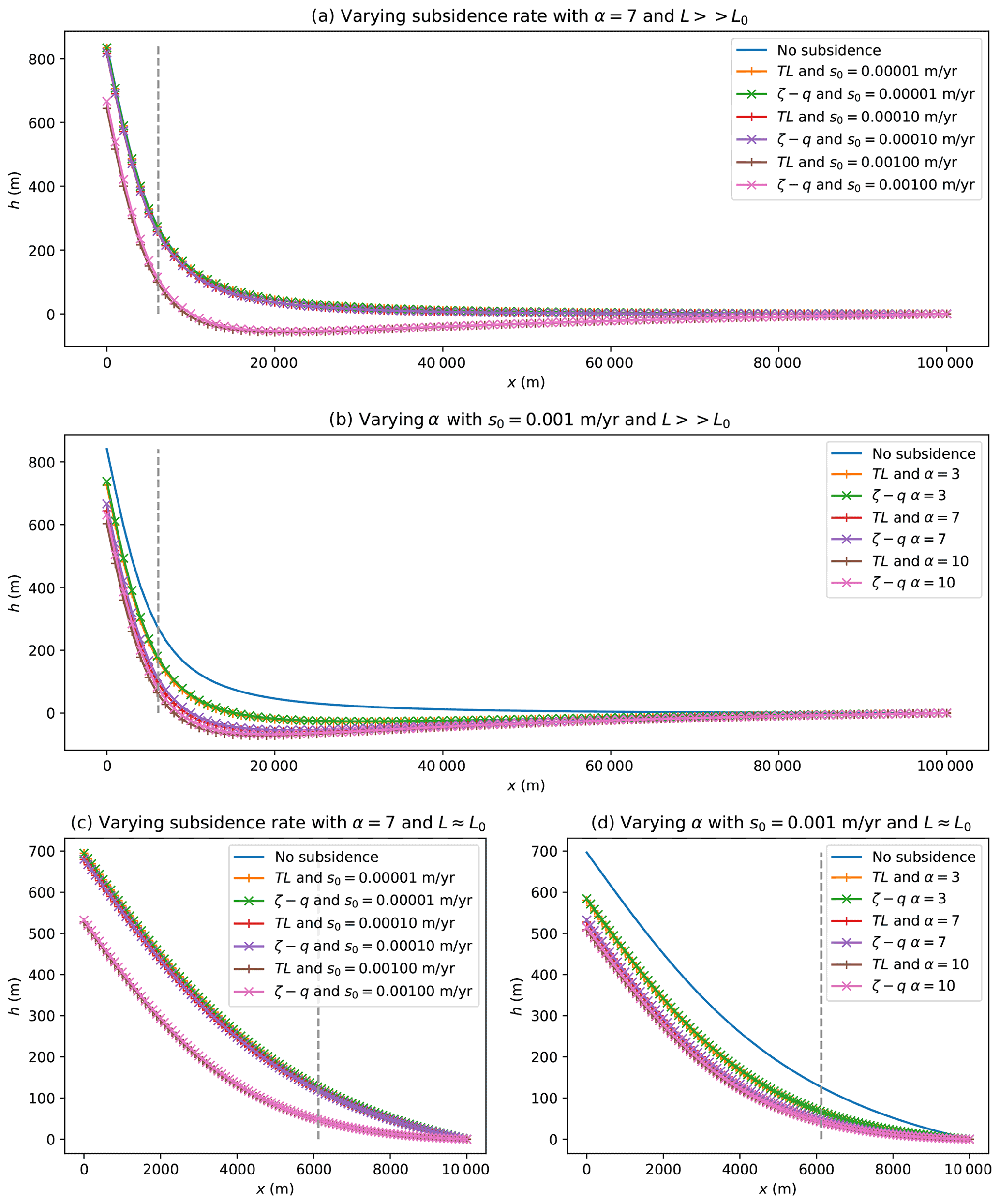
Figure 20Numerical model experiments comparing the steady-state solutions of modified versions of Eq. (3) (TL model) and Eq. (7) (ξ–q model) in which subsidence is imposed at a rate s0 and over an extent controlled by α (see text for details) to the solution without subsidence. In each panel, the dashed line corresponds to x=L0.
In Fig. 20a, I show the results of three numerical experiments in which I vary the subsidence rate by 2 orders of magnitude for a value of α of 7 for an open system (i.e., where L≫L0). In Fig. 20b, I show the results of another set of three experiments in which α is varied between 3 and 10. We see that for all values of the subsidence rate and extent, the shape of the fan and alluvial plain system is only mildly affected by the imposed subsidence. The sharp transition in slope between the fan and the alluvial plain at the location x=L0 is preserved. For constrained systems (Fig. 20c and d), the shape of the system is more strongly impacted by the subsidence. The extent of the fan is reduced when the subsidence is fast, but the extent of the subsidence function does not seem to matter much. Interestingly, in all cases the slope of the fan is not affected by the subsidence. This demonstrates that in a sedimentary system that sees discharge increase with distance from the mountain front, the size and extent of the fan, or where it connects to the alluvial plain, are only marginally controlled by the subsidence rate or extent of the underlying basement. This results applies equally to both the TL and ξ–q models.
The work I have presented here, while focused on determining the similarities and differences between the ξ–q and TL models, led me to present a new analytical solution for the steady-state shape of depositional systems fed by an orogenic system. I have shown that both models yield the same steady-state solution and that the resulting 1D profile predicts the first-order morphology of depositional systems and explains key observations made about the size and slope of alluvial fans.
From the two basic evolution equations I have also extracted expressions for the response time of sedimentary systems and shown that for model parameter values that lead to the same steady-state solution, the two models predict different response times and, most importantly, different dependencies on system length. The ξ–q model is in general characterized by longer response times than the TL model by a factor that depends on the ratio of the system drainage area to the area in active sediment transport.
I have also shown how the two different models respond to periodic variations in the imposed sediment flux from the orogenic area or in precipitation rate. These and other important findings are summarized in Table 1.
This implies that a proper understanding and parameterization of floodplain width is essential to better quantify the differences between the two models. A potential avenue for this is to use 2D versions of the two models that incorporate a proper dynamic prediction of floodplain width, which in turn requires at minimum the use of the shallow-water equation. Such models exist (Simpson and Castelltort, 2006; Davy et al., 2017, for example) but have not been used to perform this scaling analysis yet.
Using multi-direction flow-routing algorithms in landscape evolution models that do not use the shallow-water approximation and therefore imply a simple relationship between floodplain width and discharge could be useful as finite width (i.e., larger than the unit spatial discretization) seems to emerge from these models. However, more work is necessary to better characterize the transient behavior of such models and, more specifically, how channel (or floodplain) width is set (it is definitely greater than the unit spatial discretization but does not scale linearly with spatial resolution) and what determines the frequency of avulsions.
For the TL equation, I used a second-order-accurate centered scheme to approximate the spatial derivatives and a first-order-accurate implicit scheme to approximate the time derivative. For the ξ–q equation, I used a first-order-accurate scheme to approximate the spatial derivative, a first-order-accurate implicit scheme to approximate the time derivative, and the rectangle rule to estimate the integral. This yields the following discretized forms:
for the TL equation, where and , hi is current topographic elevation at node i and hi,0 is the topographic elevation at the same node at the previous time step, Δx is the distance between two nodes, Δt is the time between two time steps, and nx is the number of nodes used to discretized the river, and
for the ξ–q equation, where q0 is the incoming sediment flux (expressed in m yr−1).
These systems of equations can be written in matrix form:
where Ad and Aa are the square matrix of dimension nx×nx and Bd and Ba are vectors of dimension nx. H is the solution vector containing the topographic elevation of the nodes. For simplicity, I use a simple general direct solver for these two systems of algebraic equations even though Ad is a tridiagonal matrix and Aa is a Hessian matrix.
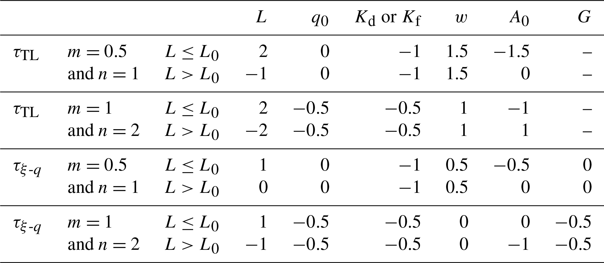
In Table B1, I illustrate this scaling for commonly assumed values of p, m and n. I consider a linear case (n=1) and a nonlinear case (n=2).
Table B1Scaling of the TL and ξ–q response times, τTL and τξ–q, with the various parameters for two sets of values of m and n. I consider a linear case (n=1) and a nonlinear case (n=2) but keep the ratio between m and n at 0.5. For both cases, I use p=2.
In the first set of experiments, I varied the erodibility, Kf, in the ξ–q equation and the transport coefficient, Kd, in the TL equation. The results are shown in Fig. C1 and demonstrate that both response times vary as the inverse of the diffusivity or erodibility, as predicted by Eqs. (23) and (27).
In a second set of experiments, I varied G, which yielded the expected scaling in the ξ–q model, as shown in Fig. C2.
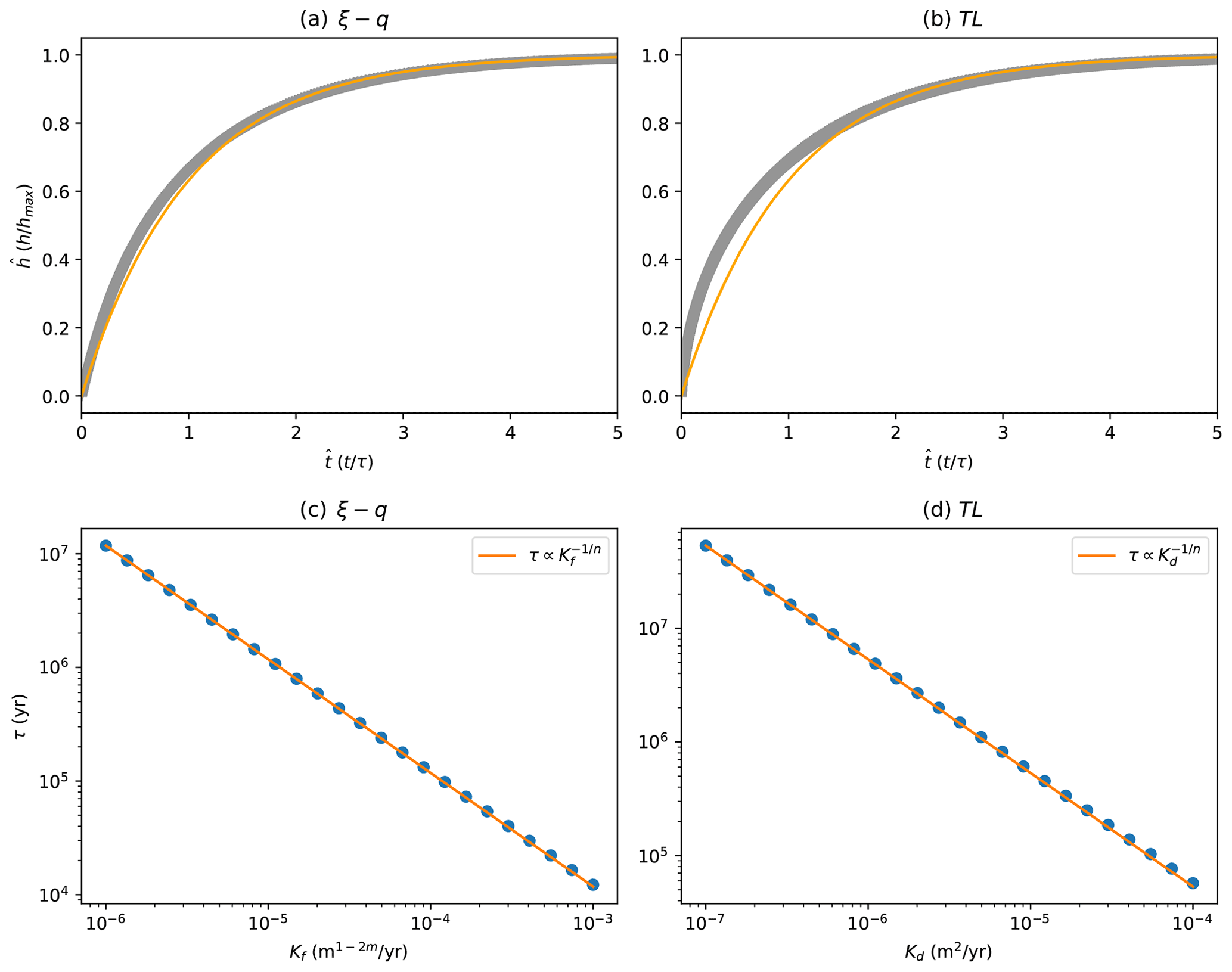
Figure C1Computed response times for 24 numerical experiments in which the erodibility, Kf, or the diffusivity, Kd, of the model were varied.

Figure C2Computed response times for 24 numerical experiments in which the deposition constant, G, of the ξ–q model was varied.
For the TL equation
and for the TL equation
The time to fill a triangle of height h0 and length L with an incoming sedimentary flux q0 is
Computations used standard finite-difference methods as described in Appendix A and performed using the Xarray–Simlab framework: https://xarray-simlab.readthedocs.io/en/latest/ (xarray-simlab, 2022).
No data sets were used in this article.
The supplement related to this article is available online at: https://doi.org/10.5194/esurf-10-301-2022-supplement.
The author has declared that there are no competing interests.
Publisher's note: Copernicus Publications remains neutral with regard to jurisdictional claims in published maps and institutional affiliations.
The author wishes to thank Sebastien Castelltort and Sebastien Carretier for comments made on earlier versions of this paper. Supported within the funding program “Open Access Publikationskosten” of the Deutsche Forschungsgemeinschaft (DFG, German Research Foundation).
The article processing charges for this open-access publication were covered by the Helmholtz Centre Potsdam – GFZ German Research Centre for Geosciences.
This paper was edited by Tom Coulthard and reviewed by Sebastien Carretier and Alexander Densmore.
Armitage, J. J., Duller, R. A., Whittaker, A. C., and Allen, P. A.: Transformation of tectonic and climatic signals from source to sedimentary archive, Nat. Geosci., 4, 1–5, 2011. a, b, c
Armitage, J. J., Jones, T., Duller, R. A., Whittaker, A. C., and Allen, P. A.: Temporal buffering of climate-driven sediment flux cycles by transient catchment response , Earth Planet. Sc. Lett., 369, 200–210, https://doi.org/10.1016/j.epsl.2013.03.020, 2013. a
Blair, T. C. and McPherson, J. G.: Processes and Forms of Alluvial Fans, Springer Netherlands, Dordrecht, 413–467, https://doi.org/10.1007/978-1-4020-5719-9_14, 2009. a, b, c, d, e
Bowman, D.: Principle of alluvial fan morphology, Springer, Dordrecht, the Netherlands, https://doi.org/10.1007/978-94-024-1558-2, 2019. a, b
Bull, W.: The alluvial fan environment, Prog. Phys. Geogr., 1, 222–270, 1977. a, b
Carretier, S., Martinod, P., Reich, M., and Godderis, Y.: Modelling sediment clasts transport during landscape evolution, Earth Surf. Dynam., 4, 237–251, https://doi.org/10.5194/esurf-4-237-2016, 2016. a, b, c
Carretier, S., Guerit, L., Harries, R., Regard, V., Maffre, P., and Bonnet, S.: The distribution of sediment residence times at the foot of mountains and its implications for proxies recorded in sedimentary basins, Earth Planet. Sc. Lett., 546, 116448, https://doi.org/10.1016/j.epsl.2020.116448, 2020. a
Castelltort, S. and Van Den Driessche, J.: How plausible are high-frequency sediment supply-driven cycles in the stratigraphic record?, Sediment. Geol., 157, 3–13, 2003. a
Davy, P. and Lague, D.: Fluvial erosion/transport equation of landscape evolution models revisited, J. Geophys. Res., 114, F03007, https://doi.org/10.1029/2008JF001146, 2009. a, b, c, d, e, f, g, h, i, j, k
Davy, P., Croissant, T., and Lague, D.: A precipiton method to calculate river hydrodynamics, with applications to flood prediction, landscape evolution models, and braiding instabilities, J. Geophys. Res., 122, 1491–1512, 2017. a
Duller, R., Whittaker, A., Fedele, J., Whitchurch, A., Springett, J., Smithells, R., Fordyce, S., and Allen, P.: From grain size to tectonics, J. Geophys. Res., 115, F03022, https://doi.org/10.1029/2009JF001495, 2010. a, b
Edmonds, D., Paola, C., Hoyal, D., and Sheets, B.: Quantitative metrics that describe river deltas and their channel networks, J. Geophys. Res., 116, F04022, https://doi.org/10.1029/2010JF001955, 2011. a
Goldberg, S. L., Schmidt, M. J., and Perron, J. T.: Fast response of Amazon rivers to Quaternary climate cycles , J. Geophys. Res., 126, e2021JF006416, https://doi.org/10.1029/2021JF006416, 2021. a
Guerit, L., Métivier, F., Devauchelle, O., Lajeunesse, E., and Barrier, L.: Laboratory alluvial fans in one dimension, Phys. Rev. E, 90, 022203, https://doi.org/10.1103/PhysRevE.90.022203, 2014. a, b, c, d, e
Guerit, L., Yuan, X.-P., Carretier, S., Bonnet, S., Rohais, S., and Braun, J.: Fluvial landscape evolution controlled by the sediment deposition coefficient: Estimation from experimental and natural landscapes, Geology, 47, 853–856, 2019. a, b, c
Henderson, F.: Open Channel Flow, MacMillan, New York, ISBN 9780023535109, 1966. a, b
Howard, A. and Kirby, G.: Channel changes in badlands, Geol. Soc. Am. Bull., 94, 739–752, 1983. a
Kooi, H. and Beaumont, C.: Escarpment evolution on high-elevation rifted margins: insights derived from a surface processes model that combines diffusion, advection and reaction, J. Geophys. Res., 99, 12191–12209, 1994. a, b
Lecce, S.: The alluvial fan problem, John Wiley and Sons, London, 3–24, 1990. a
Mouchené, M., van der Beek, P., Carretier, S., and Mouthereau, F.: Autogenic versus allogenic controls on the evolution of a coupled fluvial megafan–mountainous catchment system: numerical modelling and comparison with the Lannemezan megafan system (northern Pyrenees, France), Earth Surf. Dynam., 5, 125–143, https://doi.org/10.5194/esurf-5-125-2017, 2017. a, b
Nardi, F., Vivoni, E. R., and Grimaldi, S.: Investigating a floodplain scaling relation using a hydrogeomorphic delineation method, Water Resour. Res., 42, W09409, https://doi.org/10.1029/2005WR004155, 2006. a
Paola, C., Heller, P., and Angevin, C.: The large-scale dynamics of grain-size variation in alluvial basins, Basin Res., 4, 73–90, 1992. a
Parker, G., ASCE, M., Paola, C., Whipple, K., and Mohrig, D.: Alluvial fans formed by channelized fluvial and sheet flow!: Theory, J. Hydraul. Eng., 124, 985–995, 1998. a, b
Rhohais, S., Bonnet, S., and Eschard, R.: Sedimentary record of tectonic and climatic erosional perturbations in an experimental coupled catchment, Basin Res., 24, 198–212, 2012. a, b, c, d
Romans, B. W., Castelltort, S., Covault, J. A., Fildani, A., and Walsh, J.: Environmental signal propagation in sedimentary systems across timescales, Earth-Sci. Rev., 153, 7–29, https://doi.org/10.1016/j.earscirev.2015.07.012, 2016. a
Shobe, C. M., Tucker, G. E., and Barnhart, K. R.: The SPACE 1.0 model: a Landlab component for 2-D calculation of sediment transport, bedrock erosion, and landscape evolution, Geosci. Model Dev., 10, 4577–4604, https://doi.org/10.5194/gmd-10-4577-2017, 2017. a
Simpson, G. and Castelltort, S.: Coupled model of surface water flow, sediment transport and morphological evolution, Comput. Geosci., 32, 1600–1614, 2006. a, b
Tofelde, S., Bernhardt, A., Guerit, L., and Romans, B. W.: Times Associated With Source-to-Sink Propagation of Environmental Signals During Landscape Transience, Front. Earth Sci., 9, 628315, https://doi.org/10.3389/feart.2021.628315, 2021. a
Whipple, K. and Tucker, G.: Dynamics of the stream-power incision model: implications for height limits of mountain ranges, landscape response timescales and research needs, J. Geophys. Res., 104, 17661–17674, 1999. a
Whipple, K., Parker, G., Paola, C., and Mohrig, D.: Channel Dynamics, Sediment Transport, and the Slope of Alluvial Fans: Experimental Study, J. Geol., 106, 677–693, 1998. a, b, c, d, e
xarray-simlab: Xarray extension for computer model simulations, https://xarray-simlab.readthedocs.io/en/latest/, last access: 25 March 2022. a
Yuan, X. P., Braun, J., Guerit, L., Rouby, D., and Cordonnier, G.: A New Efficient Method to Solve the Stream Power Law Model Taking Into Account Sediment Deposition, J. Geophys. Res., 124, 1346–1365, https://doi.org/10.1029/2018jf004867, 2019. a, b, c, d, e
- Abstract
- Introduction
- Method
- Results
- Discussion
- Conclusions and perspectives
- Appendix A: Numerical method to solve the two equations assuming n=1
- Appendix B: Response time scaling for various values of m and n
- Appendix C: Validation of response timescale relationship
- Appendix D: Expressions for the flux
- Appendix E: Geometrical interpretation of the response time
- Code availability
- Data availability
- Competing interests
- Disclaimer
- Acknowledgements
- Financial support
- Review statement
- References
- Supplement