How ice apron loss and permafrost degradation promoted the Platteikogel rock slope failure: a thermo-mechanical reconstruction

The Alpine cryosphere changes at unprecedented speed, affecting the thermal, hydrological, and mechanical state and behaviour of rock slopes. While numerous studies investigated singular drivers for progressive rock slope failures, the knowledge of hydro-thermo-mechanically coupled processes remains scarce. In this paper, we investigate the 2024 permafrost rock slope failure at Platteikogel with a volume of 50 000 m³ (3395 m a.s.l., above Vernagtferner, Austria). We aim to assess how observed ice apron loss and related permafrost warming promote the release mechanism. We reconstructed multidecadal thermal evolution accounting for the thermal impact of ice apron loss. Based on field observations, we derived a conceptual model on how ice apron loss potentially affects rock slope destabilization. Integrating the outcome of the preceding steps, we performed a mechanical stability analysis assuming that the rock slope failed along ice-filled discontinuities. The mechanical model indicates that the failure can not be solely explained by a warming-driven decrease in shear strength of ice-filled discontinuities, suggesting that other failure processes superimpose or even dominate. The implemented system feedback related to ice apron loss suggests that hydrostatic pressure buildup due to water infiltration and rockfall-induced unloading thereby promoted the Platteikogel rock slope failure. In summary, we demonstrate that ice apron loss not only leads to increased rockfall activity but also accelerates progressive failure, promoting the detachment event. In upcoming decades, ice aprons on steep rock slopes above 3000 m in the European Alps are expected to experience drastic area loss, exposing potential source zones for future rock slope failures.

1 Introduction

Recent rock slope failures in the cryosphere of the European Alps underscore both the anticipated increase in frequency under a warming climate (Intergovernmental Panel on Climate Change, 2022) and the complexity of the failure processes: Notable examples include the permafrost rock slide at Fluchthorn (Austria, 2023; Krautblatter et al., 2024), the rock slide beneath glacier ice at Piz Scerscen (Switzerland, 2024; Pierhöfer et al., 2024), and the complex glacier failure at Blatten which was preceded by permafrost-related rockfalls (Switzerland, 2025; Islam et al., 2025). All of these failures evolved into multi-kilometer, highly mobile rock–ice avalanches, illustrating the potential – or, in the case of Blatten, the actual – threat posed to valley populations by cascading processes.

While rock slope destabilization mechanisms have been investigated for changes in glaciers (Fischer et al., 2010; Rechberger and Zangerl, 2022; Walden et al., 2025) or permafrost (Gruber and Haeberli, 2007; Phillips et al., 2017; Etzelmüller et al., 2022), less attention has been drawn towards ice aprons. Ice aprons – defined as irregularly shaped, small ice bodies – typically less than 0.1 km² in area and located on slopes steeper than 40° – undergo rapid area loss in the 21st century, and have almost exclusively been studied in the Western Alps (Ravanel et al., 2023). While glaciers retreat from the bottom up, the upper boundary of ice aprons shifts top-downwards, as observed during continuous area loss. Over a 70-year observation period (1952–2019) in the Mont Blanc Massif, the area of ice aprons has declined by 47 % (Kaushik et al., 2022). Ice apron loss is hypothesized to negatively impact the stability of permafrost rock slopes by inducing thermo-mechanical alteration upon their disappearance (Guillet and Ravanel, 2020), however, the actual processes remain poorly constrained.

In this paper, we aim to decipher the failure mechanism of the Plateikogel rock slope failure (3395 m a.s.l., release volume of 50 000 m³, spring 2024, situated in the Vernagtferner Basin, Tyrol, Austria). The rock mass detached from a ridge flanked by glaciers. Ice aprons reached the detachment area in 1970 but have since lost substantial elevation. We investigate the destabilization of the rock slope combining three complementary steps: (i) Analysis of visible cryospheric and geomorphic changes, (ii) modeling decadal permafrost evolution using the conductive heat flow model (CryoGrid 2D; Czekirda et al., 2023), and (iii) modeling rock slope mechanics with distinct element code (UDEC; Itasca Consulting Group, 2019), integrating (i) and (ii) to assess the mechanical impacts associated with the paraglacial transition (Fig. 1).

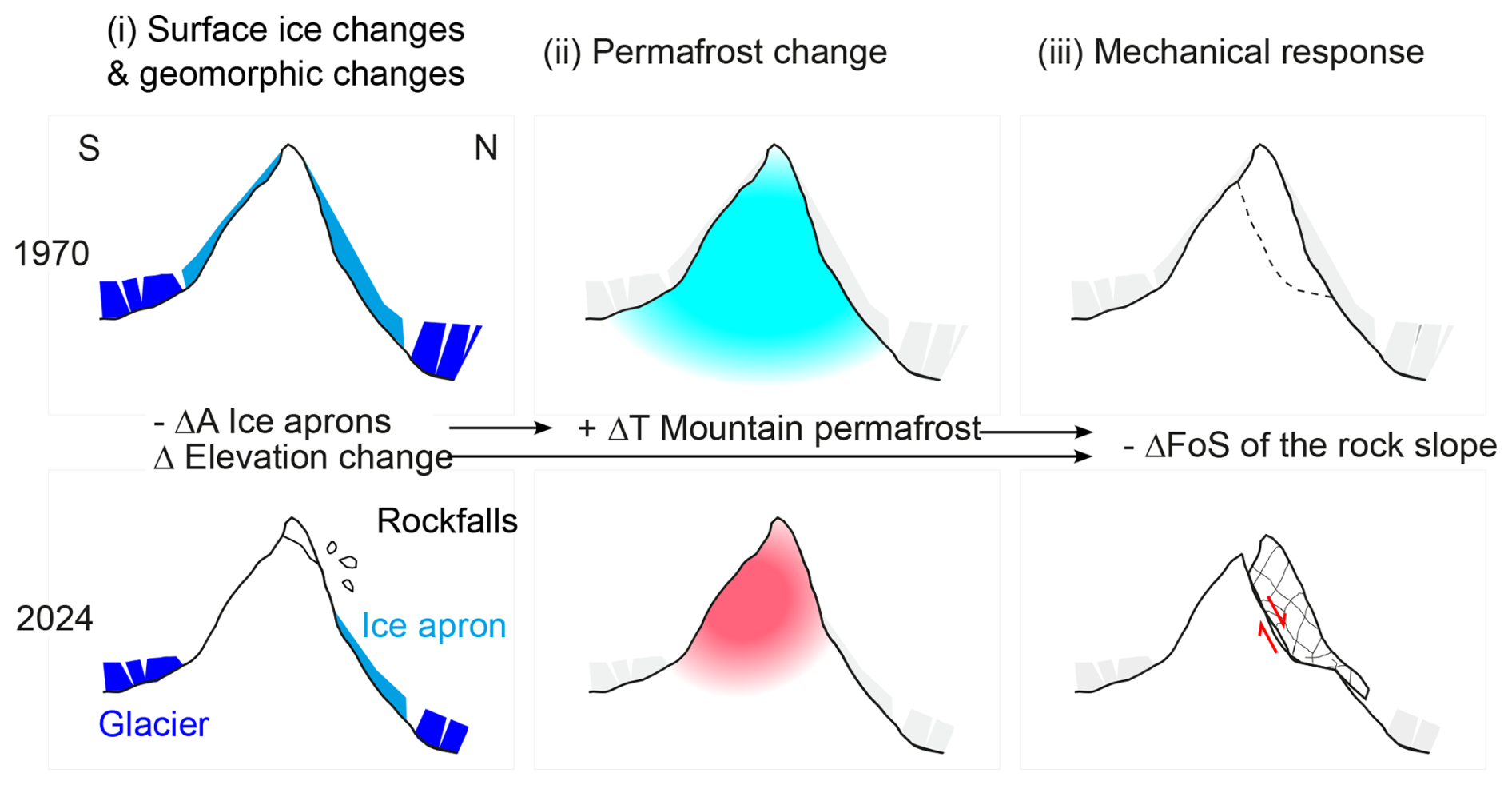
Figure 1 Conceptualized workflow of this study, which iterates from (i) observing surface ice changes and geomorphological changes to (ii) permafrost modeling to (iii) mechanical investigations of rock slope stability. The expected changes Δ within the observation period of more than four decades are illustrated. Abbreviation: A – Area, T – Temperature, FoS – Factor of safety. Arrows indicate result transfer used as input for subsequent modeling.

This multi-method study is the first to apply a laboratory-derived rock–ice mechanical shear model to an actual rock slope failure at slope scale, challenging its applicability to larger scales. Furthermore, we demonstrate the thermal impact of ice apron loss on permafrost warming and propose a conceptual model describing the feedbacks between ice apron loss and rock slope destabilization. This study aims to provide an integrated understanding of the coupled thermo-hydro-mechanical processes that promote rock slope failures in permafrost.

We address the following questions:

• i.

  How does the area loss of the ice apron affect the thermal state of permafrost at the Platteikogel?

• ii.

  Assuming ice-filled fractures, did climate-driven permafrost warming contribute to the destabilization and release of the rock slope?

• iii.

  Which other mechanisms were relevant in the final phase of slope failure?

In this paper, we follow the landslide terminology of Hermanns et al. (2022) and use the term rock slope failure to describe landslides with detachment in rock, independent of failure kinematics. This term encompasses the pre-failure deformation and associated geomorphic activity, the main failure event (sudden failure), and the post-failure deformation or related geomorphic activity. The spatial data and time series used for the analysis presented in this publication are summarized in the Tables A1 and A2.

2 Characterization of the field site

2.1 The Platteikogel rock slope failure

The Platteikogel rock slope failure (46°52^′14.2^′′ N 10°50^′46.2^′′ E) occurred on a NE-SW-oriented mountain ridge at 3400 m a.s.l. surrounding the Vernagtferner glacier, Ötztal, Tyrol, Austria; Glacier ID: 489 (World Glacier Monitoring Service, 2025). The affected area and deposits are shown on aerial photographs and the slope map in Fig. 2. The exact timing of the event remains unclear and can only be narrowed down to the period between 25 April and 6 June 2025 (Sentinel-2 L2A; European Space Agency, 2024). No seismic or hydrological recordings in the near surroundings indicate any unambiguous signals related to the event. Landslide-related metrics are given in Table 1.

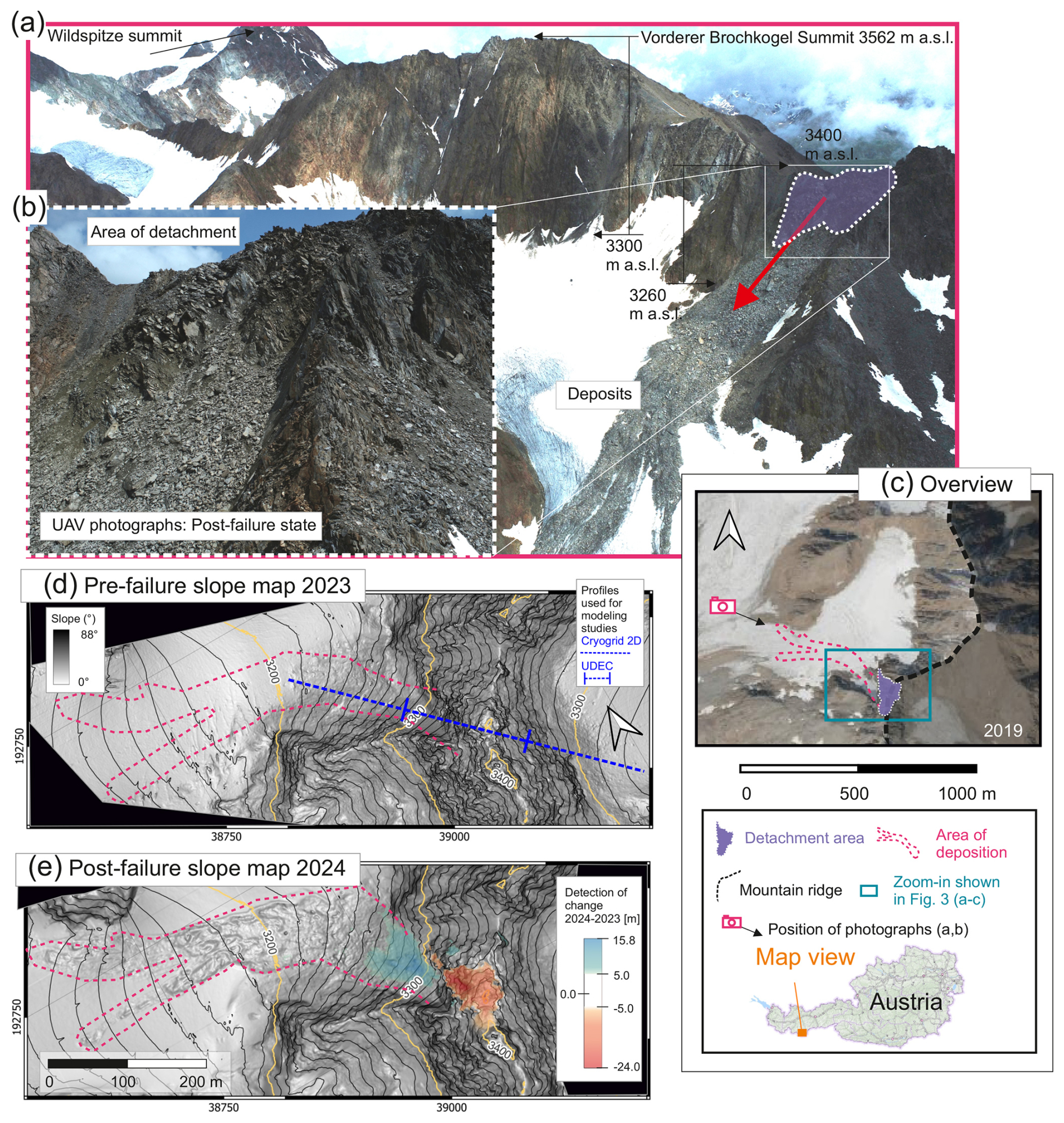
Figure 2 (a) Aerial view from NW showing the full dimensions of the affected area at post-failure state, and (b) zoom-in to the detachment area. Both photographs (a, b) were captured by a UAV on 8 August 2024. (a) From the macro perspective, the steep and vertical gullies incised in the headwall of the Vorderer Brochkogel summit clearly demonstrate the tectonic structure of the foliated metamorphic rock mass. (b) The shape of the individual boulders and blocks of the disintegrated rock mass is slab-like according to the foliation structure. Distinct zones with a high concentration of fine grains are visible in the detachment zone. (c) Overview of the location and extent of the Platteikogel rock slope failure situated in the cirque of the Kleiner Vernagtferner. (d) Slope map at pre-failure state, including the profiles used for modeling studies. (e) Slope map at post-failure state showing the morphology of deposition, and the change detection (threshold of detection: 5 m). Data source: (c) Orthophotography acquired by Land Tirol – https://www.tirol.gv.at/data/ (last access: 7 January 2025).

Table 1 Classification and metrics regarding the Platteikogel rock slope failure.

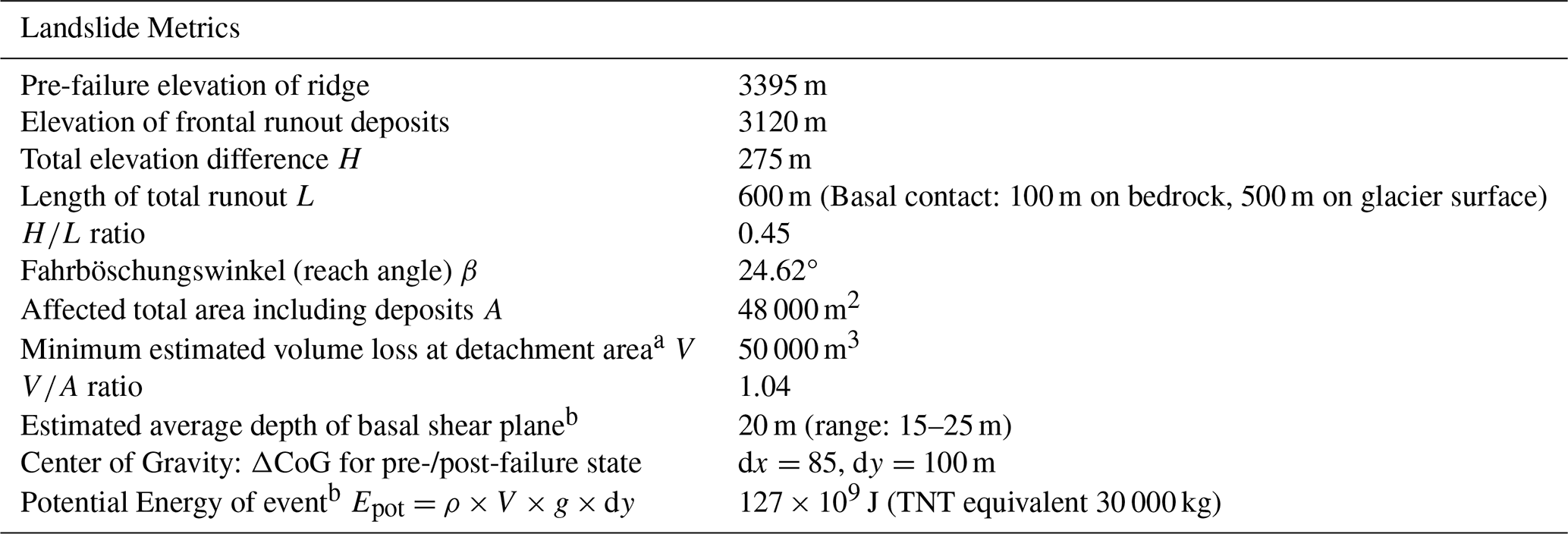
^a Change detection was conducted for the point clouds of 2023 and 2024 (each 2 cm resolution) at the detachment area only. The volume error is smaller than 100 m³. ^b Assumed ρ=2600 kg m⁻³.

The geology at the detachment area consists of schistose gneiss with feldspar augen and staurolite minerals, enclosing a local intersection of muscovite schist in the direct vicinity of the South of the detachment area (Geologische Bundesanstalt Österreich, 2021). Structural geology was likely to favor the destabilization of the Platteikogel rock slope (Fig. A1 – analysis of rock outcrops): The pronounced foliation of the metamorphic rock is visible from afar, marking the many incised gullies in the steep wall (Fig. 2a). The foliation exhibits a general dip direction toward S/SSE and steep dip angles ranging from 60 to 85°. Moreover, two prominent, non-foliation parallel joint sets were identified, both striking nearly perpendicular to the direction of rock slope displacement. Their dip directions are northwest and southeast. General joint spacing ranges from centimeters to several decameters up to meters and varies locally. Although the dip angles of both joint sets (ranging between 60 to 80°) are generally steeper than the slope angle, suggesting that sliding is inhibited by geometry, the narrow joint spacing likely favored a step-path shear failure (Eberhardt et al., 2004). Slab-shaped, disintegrated, angular blocks characterize the detachment area at post-failure state (Fig. 2b).

2.2 Cryospheric changes and pre-failure rockfall activity

Glaciers surround both sides of the ridge of the detachment area, with ice aprons extending steeply upwards below the ridge crest. Given that a dynamic cryosphere affects rock slope mechanics through changes in water availability, temperature, and local stress field (ice loss/rockfalls), the subsequent paragraphs focus on the evolution of the cryosphere in the area of the detachment.

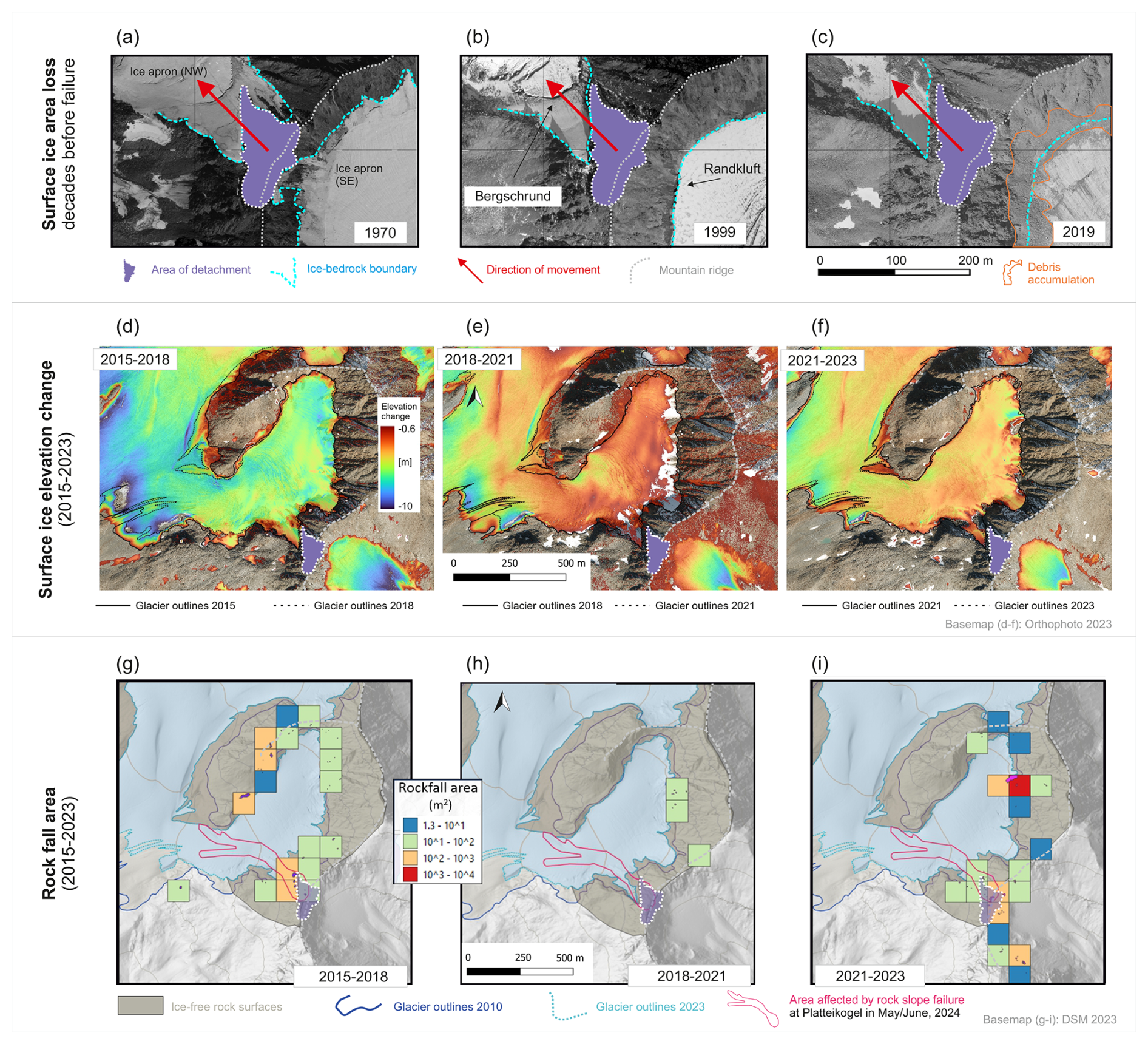
Figure 3 (a–c) Changes in ice cover 5 decades before failure, (d–f) surface ice elevation change, and (g–i) affected rockfall area years before failure shown for the area of Platteikogel rock slope failure (for location of analyzed area see Fig. 2a). The spatio-temporal surface ice changes (d–f) and rockfall inventory (g–i) were processed following the approach for multi-temporal quantification of surface changes described in the Supplement of Barbosa et al. (2024). (d–f) Glacier outlines were mapped manually on orthophotos with 20 cm resolution for the respective years. The limit of detection was set to −0.6 m. Note: Due to changes made to the camera system in the 2021 campaign, panel (e) shows artifacts due to the suboptimal model alignment, such as the pronounced scattering at the SE exposed slopes in the lower right. (g–i) Spatial distribution of rockfall activity at the ridges surrounding the Kleiner Vernagtferner. Rockfalls are manually mapped using geomorphic change detection from a DSM derived from aerial imagery at 20 cm spatial resolution. We used a 100 m grid to display the cumulative rockfall area in m² per time interval. The glacier extent was manually mapped. Data sources: (a–c) orthophotography acquired by Land Tirol – https://www.tirol.gv.at/data/, (d–i) large-format aerial imagery acquired by 3D RealityMaps GmbH.

The detachment area lies within permafrost (100 % probability of permafrost occurrence according to permafrost distribution map; Otto et al., 2020). Moreover, the presence of ice aprons indicates subzero rock surface temperatures (Benn and Evans, 2014). Figure 3a–c demonstrates the visible changes of ice aprons at the detachment area in past decades (ice apron typology: steep ice apron above glacier, cf. Fig. 1 (4) in Ravanel et al., 2023): Between 1970 and 1999, the upper limit of ice aprons decreased to the position of the former Bergschrund, losing more than 50 m in elevation at the southeastern flank of the ridge. In the period 1999 to 2019, the recent ice-free bedrock exhibits incised gullies, while debris cones accumulated on the glacier below. In contrast, the ice apron at the northwestern flank exhibits less loss in area, but shows overall derogation, with widening of the berschrund, and opening of crevasses underneath in 1999. For the period analyzed (1970–2019), the Bergschrund at the northwestern flank remained almost in a stationary position (±5 m).

Analyzing surface ice elevation changes of Kleiner Vernagtferner located northwest of the ridge in the years before failure from 2015 onwards, a rate of elevation change > 3 m yr⁻¹ was calculated for the lower part of the glacier, while a rate of elevation change of ≈ 0.3 m yr⁻¹ was calculated for the area of ice aprons. Similar values were derived for the Platteiferner located southeast of the ridge (Fig. 3d–f). While ice aprons were in direct contact with the rock in the detachment area, both glaciers were situated more than 50 m below. Focusing only on the uppermost area of ice aprons, the analyzed data suggests a loss of at least 5 m of ice apron thickness in the decade before the failure in 2024.

Together with observed changes in surface ice, rockfall activity was evident in the detachment area since 2015 onwards (Fig. 3g–i): Between 2015–2018, seven rockfalls occurred (561 m² total; 5–311 m² each). No events were detected from 2018–2021. From 2021–2023, fourteen rockfalls occurred (412 m² total; 2–236 m² each).

3 Methodological approach

An extended map view, including the positions of all meteorological stations from which data were used for the thermal modeling conducted subsequently, is shown in Fig. S1 – the label S denotes Supplement. The cross-section selected for the modeling studies follows the direction of mass movements and runs perpendicular to the mountain's ridge. Its topography was inferred from the pre-failure digital elevation model of 2023 (Table A1, i, for location see Fig. 2d) and was smoothed to a step width of 5 m.

3.1 Modeling the thermal evolution of the mountain ridge

We use the transient conductive heat flux model CryoGrid 2D, which was applied in other studies on permafrost evolution in steep rock walls (Myhra et al., 2017, 2019; Czekirda et al., 2023), in order to reconstruct permafrost conditions in the decades before the rock slope failure event in 2024. With Cryogrid 2D, the subsurface temperature field is calculated by solving the heat diffusion equation following Fourier's law of heat conduction according to defined material- and temperature-dependent parameters. The finite element solver MILAMIN package (Dabrowski et al., 2008) was employed to numerically solve complex geometries on unstructured grids, based on specified boundary conditions and the imposed temperature forcing along the model topography. Time discretisation follows a finite-difference backward Euler scheme. A detailed description of the CryoGrid 2D model is provided by Myhra et al. (2017). Here, we use the Cryogrid 2D version as applied by Czekirda et al. (2023). The modeling strategy follows their approach and is outlined below.

3.1.1 Model calibration and setup

First, we calibrated the thermal parameters with measured borehole data: We assumed uniform rock mass properties (single lithology according to field observations). The volumetric fraction of rock and water was set to 0.95 and 0.05, accounting for fractured and jointed gneissic rock mass (Myhra et al., 2017, 2019). We calibrated the parameters thermal conductivity k, and volumetric heat capacity c_v with measured temperatures of the borehole at Matterhorn (PERMOS, 2024), which has similar lithology and altitude to the Platteikogel detachment area. Therefore, we utilized a simplified column mesh and horizontal model topography, and applied a uniform heat flux of 50 mW m⁻² at 6000 m depth. The model was then forced using measured temperatures at 0.1 m depth. Measured borehole temperatures at greater depths were compared with the simulated temperature profiles (Fig. A2a1–a4). The configuration of parameters resulting in the best model-fit (compare Fig. A2a1–a4) was selected for all further simulations: k=2 W K⁻¹ m⁻¹, $c_{\mathrm{v}}=\mathrm{3}\times {\mathrm{10}}^{\mathrm{6}}$ J m⁻³ K⁻¹. For the simulation regarding the Platteikogel rock slope failure, we constructed an unstructured triangular mesh using the smoothed cross-section profile of the mountain ridge by using the Triangle library (Shewchuk, 1996). The node density was decreased gradually with higher depth (see Table S1). Aforementioned calibrated parameters were prescribed to the entire Platteikogel mountain.

3.1.2 Applied forcings

Figure 4 illustrates the cross-section with varying surface types, indicating their thermal functionality regarding permafrost in the rock mass below. To simulate the thermal evolution of the Platteikogel ridge, we forced the model using mean monthly rock surface temperatures (RST), which were projected along the rock topography. RSTs are obtained from air temperatures (AT); their difference defines the surface offset (SO). First, we created a long-term dataset of monthly AT for the site of Platteikogel: Mean monthly lapse rates were calculated using the temperature records (2003–2024) from two nearby meteorological stations (i), at 2863.9 m a.s.l., and (ii), at 3437 m a.s.l. (GeoSphere Austria, 2024). Second, linear regression models were applied to extrapolate the temperature time series for station (ii), using (iii) historical mean monthly air temperature records from long-term monitoring station Obergurgl (Auer et al., 2007), which is located at 1938 m a.s.l. in the neighboring valley. This resulted in a mean monthly AT time series for the period 1900 to 2024, corresponding to the approximate elevation of the detachment area. Thirdly, the calculated lapse rates were used to adjust the monthly AT values to the corresponding elevations along the profile (for station details see Table A2, i–iii).

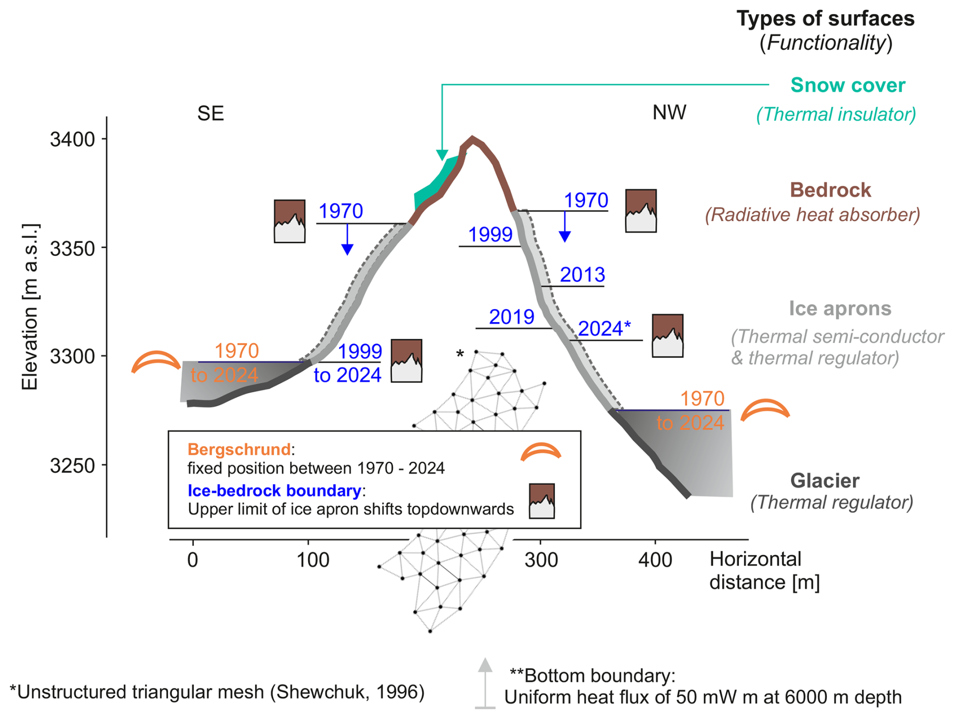
Figure 4 Cross-section through the ridge of Platteikogel, demonstrating varying surface types and the observed downslope retreat of ice apron since 1970 onwards – Given dates/elevation marks are inferred from historic orthophotographs. The topography (upper boundary) and lower boundary (implied, at 6000 m depth) mark the frame for the meshed model. Note: The vertical scale of the cross-section is exaggerated by a factor of 2.

On the basis of AT, we inferred RST for varying surface types along the profile – bedrock, snow cover, ice aprons, and glacier ice – by using temperature transfer functions. Accounting for natural variability and uncertainty in SO, we specified a plausible range of values for the sampling of ensemble simulations. These functions are explained in the following. Examples for the application of these functions are demonstrated in Fig. S2a–e.

• i.

  Seasonal snow cover: Seasonal snow cover acts as a thermal insulator, buffering cold AT signals (Haberkorn et al., 2015). Snow reduction factors nF [–] (Smith and Riseborough, 2002; Gisnås et al., 2013) were multiplied with negative AT for months with snow cover only (assumed period of snow cover: 1 November to 31 May, Fig. S2b). For positive AT in this period, we enforced an isothermal snow cover with 0 °C. Following Czekirda et al. (2023), we used the slope of the profile to assess the nF-factors ranging from 0.5 for slope < 30° to 1 for slope > 60° along the profile topography and calculated RST below the snow cover using the empirical transfer function (see Fig. S3):

  $$\begin{array}{}\text{(1)}& \begin{array}{rl}& {\mathrm{RST}}_{\text{snow cover}}=\\ & \left\{\begin{array}{l}\mathrm{AT}\cdot \left(\mathrm{nF}\right(\text{slope})+x),\\ \text{if }\mathrm{AT}<\mathrm{0}\mathit{°}\mathrm{C},x\in [-\mathrm{0.1},\mathrm{0.1}],\\ \mathrm{0}\mathit{°}\mathrm{C},\text{if }\mathrm{AT}\ge \mathrm{0}\mathit{°}\mathrm{C}.\end{array}\right.\end{array}\end{array}$$
• ii.

  Bedrock: Snow-free, sun-exposed rock surfaces undergo significant radiative warming (Magnin et al., 2019). For snow-free locations with either slope angles > 60° or during the snow-free months, we calculated the RST using fixed temperature offsets accounting only for the aspect of the mountain flank (Fig. S2b). The here defined surface offset range chosen for radiative warming of rock surfaces is consistent with measured data (Czekirda et al., 2023, rock walls in Norway), and calculated RST-AT offsets on the basis of measurements from the Matterhorn Hörnli ridge, Switzerland, 3500 m a.s.l. (see Fig. S4, data source: Weber et al., 2024).

  $$\begin{array}{}\text{(2)}& \begin{array}{rl}& {\mathrm{RST}}_{\mathrm{exposed}\mathrm{rock}}=\\ & \left\{\begin{array}{ll}\mathrm{AT}+{\mathrm{SO}}_{\mathrm{NW}},& {\mathrm{SO}}_{\mathrm{NW}}\in [-\mathrm{1},+\mathrm{1}]\mathit{°}\mathrm{C},\\ \mathrm{AT}+{\mathrm{SO}}_{\mathrm{SE}},& {\mathrm{SO}}_{\mathrm{SE}}\in [+\mathrm{2},+\mathrm{4}]\mathit{°}\mathrm{C}.\end{array}\right.\end{array}\end{array}$$
• iii.

  Ice aprons: Ice aprons insulate the rock in summer due to the lower thermal diffusivity of warm ice, and limit warming above 0 °C by latent heat consumption during the surface melt. In winter, they enhance the cooling of the bedrock by the relative increase of diffusivity of colder ice (James, 1968). Temperatures measured at depths between 2.5 and 8.8 m of a NNE-facing ice apron at 3470 m a.s.l. at Tour Ronde (France) show that mean annual temperatures strongly converge at −5 ± 0.5 °C regardless of the depth in the mentioned range (Ravanel et al., 2023). While the seasonal air temperature signal is pronounced at shallow depths, it exhibits only a marginal amplitude at 8.8 m depth. For the modeling strategy, we assume that ice aprons, for their entire vertical extension, consist of uniform thickness. To account for the thermal effect of ice aprons on the rock surface underneath, we implemented a low-pass filter on the basis of the analytical solution of the 1D conductive heat equation (Carslaw and Jaeger, 1980), which dampens monthly fluctuations of AT with increasing ice thickness, while annual signals penetrate deeper (Fig. S2c; approximating the observed results of Ravanel et al., 2023). Using properties of ice: ρ_ice=917 kg m⁻³, k_ice=2.1 W m⁻¹ K⁻¹, c_ice=2009 J kg⁻¹ K⁻¹, and assuming uniform thickness of ice $H_{\mathrm{ice}}\in [\mathrm{1},\mathrm{9}]$ m throughout the entire simulation time, we calculate the damping factor: $e^{-H_{\mathrm{ice}}/\mathit{\delta }}$, with penetration depth $\mathit{\delta }=\sqrt{\mathrm{2}\mathit{\kappa }/{\mathit{\omega }}_y}$, ${\mathit{\omega }}_y=\mathrm{2}\mathit{\pi }/(\mathrm{365}\cdot \mathrm{24}\cdot \mathrm{3600})$ s and diffusivity $\mathit{\kappa }=k_{\mathrm{ice}}/({\mathit{\rho }}_{\mathrm{ice}}\cdot c_{\mathrm{ice}})$. The formula used to calculate the monthly temperature at the rock-ice arpon interface is

  $$\begin{array}{}\text{(3)}& \begin{array}{rl}& {\mathrm{RST}}_{\mathrm{ice}\mathrm{aprons}}=min({\mathrm{TIAS}}_{\mathrm{mean}}\\ & +e^{-H_{\mathrm{ice}}/\mathit{\delta }}[{\mathrm{TIAS}}_m-{\mathrm{TIAS}}_{\mathrm{mean}}],\mathrm{0}\mathit{°}\mathrm{C})\\ & H_{\mathrm{ice}}\in [\mathrm{1},\mathrm{9}]\mathrm{m}\end{array}\end{array}$$

  Note that the minimum statement introduced in the formula limits the monthly temperature at the rock-ice apron interface to a maximum of 0 °C. Here, TIAS refers to the Temperature at the Ice Apron Surface specified for a location of 0.1 m below the current ice surface (analogous to the standard depth specified for RST measurements). It serves to calculate the RST_ice aprons and is calculated as follows.

  Monthly temperature at ice apron surface…

  $$\begin{array}{}\text{(3a)}& \begin{array}{rl}& {\mathrm{TIAS}}_m=\\ & \left\{\begin{array}{ll}{\mathrm{RST}}_{\mathrm{snow}}\left(m\right),& \text{if }m\in \mathit{\{}\mathrm{1},\mathrm{2},\mathrm{3},\mathrm{4},\mathrm{5},\mathrm{11},\mathrm{12}\mathit{\}},\\ & \text{snow cover on top of ice}\\ & \text{apron}\to \text{Eq. (1)},\\ \mathrm{AT}\left(m\right),& \text{otherwise, ice apron surface }\\ & \text{exposed}\to \text{no surface}\\ & \text{offset};\end{array}\right.\end{array}\end{array}$$

  Mean annual temperature at ice apron surface calculated for each year respectively…

  $$\begin{array}{}\text{(3b)}& {\mathrm{TIAS}}_{\mathrm{mean}}={\displaystyle \frac{\mathrm{1}}{\mathrm{12}}}\sum _{m=\mathrm{1}}^{\mathrm{12}}{\mathrm{TIAS}}_m.\end{array}$$
• iv.

  For the glacier below the ice aprons – the Bergschrund marks the transition – we assumed rather thin glacier ice in the order of a few decameters, with marginal movement. However, the glacier may distinctly differ from the ice apron by its greater thickness of the ice body. In the areas near the headwalls of the cirque, the ice might still be frozen to bedrock (Benn and Evans, 2014). For the simulation, we assume thick perennial snow cover on top of the glacier, using a fixed nF-factor throughout the entire simulation time, and suggest that the ice thickness is well beyond the depth of the seasonal penetration signal (Fig. S2d). Monthly glacier-bed temperatures were calculated from the mean annual air temperature (MAAT) as:

  $$\begin{array}{}\text{(4)}& {\mathrm{RST}}_{\mathrm{glacier}}=\mathrm{MAAT}\cdot \mathrm{nF},nF\in [+\mathrm{0.4},+\mathrm{0.6}]\end{array}$$

Apart from AT, we considered the gradual retreat in ice apron since 1970 (Figs. 2a–c and 4) as a dynamic variable in our model, while snow cover, solar radiation, and glacier extent were treated as static throughout the simulation period. We therefore implemented a linearly decreasing ice-bedrock boundary for the southeastern flank from 1970 at an elevation of 3355 m a.s.l. to 1999 at an elevation of 3290 m a.s.l. For the northwestern flank, the ice-bedrock boundary decreased from 1970 at an elevation of 3365 m a.s.l. to 2024 at an elevation of 3310 m a.s.l. (Fig. S5). In our simulation, only two states are considered: Ice aprons of constant thickness throughout their existence and extent, or ice-free surfaces following top-down retreat. For the newly exposed ice-free surfaces, RSTs were calculated respecting snow cover and radiative bedrock warming (Eqs. 1 and 2; Fig. S2e). In contrast to the varying ice apron extent, the glacier in the area of the cirque, delimited by the observed stationary bergschrund (±5 m in horizontal direction between 1970 and 2023), was considered stationary, and its temporal variations in thickness were ignored. Before 1970, we assumed the glacier and ice apron extent to be identical to the 1970 extent.

3.1.3 Simulation strategy

The model was initialized with the mean annual RST of 1900 (calculated with the mean of the values in defined ranges in Eqs. 1 to 4) along the model topography and the geothermal heat flux at the bottom boundary until a steady state was reached within the model domain (marginal difference of modeled temperature between consecutive years of less than 10⁻⁴ °C). Starting from the initialized state in 1900, we ran 100 individual simulations until 2024 in order to account for uncertainties through the use of temperature transfer functions. Each simulation was forced with RST calculated on basis of randomly sampled offset parameters within specified ranges: Eq. (1): $x\in [-\mathrm{0.1},\mathrm{0.1}]$; Eq. (2): ${\mathrm{SO}}_{\mathrm{NW}}\in [-\mathrm{1},+\mathrm{1}]$, ${\mathrm{SO}}_{\mathrm{SE}}\in [+\mathrm{2},+\mathrm{4}]$ °C; Eq. (3): $H_{\mathrm{ice}}\in [\mathrm{1},\mathrm{9}]$ m; Eq. (4): $\mathrm{nF}\in [+\mathrm{0.4},+\mathrm{0.6}]$. The full workflow following (a) model calibration, (b) setup, (c) surface forcings, to (d) simulation strategy is comprised in Fig. A2.

3.2 Mechanical modeling of the failure mechanism

3.2.1 The mechanical implications of ice apron loss

Based on our observations of ice apron retreat (Sect. 2.2), we derive a conceptual model emphasizing the coupled effects on (i) permafrost degradation, (ii) hydrogeology, and (iii) topographic modification through rockfall activity (Fig. 5), which in turn influences rock slope stability. The concept explained here serves to define the simulation scenarios for the rock mechanical analysis of the Platteikogel rock slope failure.

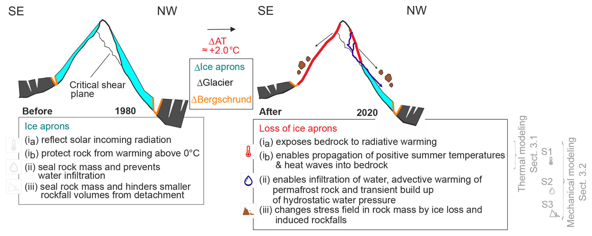
Figure 5 Conceptual model indicating the impact of ice apron loss on (i) permafrost, (ii) hydrogeology, (iii) geomorphic processes. The glacier and ice apron thickness is sketched arbitrarily. The lower right comprises the processes that are investigated by mechanical modeling in this paper. Note: (i) Contrast in albedo (snow/ice ≈ 0.2–0.9; rock ≈ 0.05–0.2) and thermal response (ice limited to 0 °C; rock potentially warms beyond melting point). (ii) Very low ice permeability ($k_{\mathrm{ice}}\approx {\mathrm{10}}^{-\mathrm{18}}$ m⁻²). (iii) Topographic change and mass loss may raise effective stress σ_eff. beyond critical stress σ_crti..

We briefly address the consequences of ice apron loss on the various systems:

• i.

  Upon ice apron retreat, newly exposed surfaces are subject to increased radiative heating and sensible heat exchange (Deline et al., 2015). From now on, an active layer might seasonally be formed, enhancing permafrost degradation.

• ii.

  Ice that once sealed the bedrock, preventing rain or meltwater from infiltration, vanishes and makes the uppermost bedrock more permeable. As a result, water infiltration can lead to the buildup of hydrostatic water pressure within the rock mass (Offer et al., 2025; Scandroglio et al., 2025).

• iii.

  The upper meters of exposed bedrock experience a thermal shock by regular freeze-thaw cycles, which lead to accelerated fatigue of rock and weathering processes (Jia et al., 2015), resulting in increased rockfall events (Draebing and Mayer, 2021).

The system exhibits a strong feedback loop with coupled interdependencies: In fractured permafrost rock, both conductive and advective thermal transport processes are relevant (i ↔ ii). The latter typically channels energy transport by water flow paths along fractures, forming local thaw corridors resulting in heterogeneous permafrost zones (Hasler et al., 2011; Magnin and Josnin, 2021). Hydrostatic pressure (ii) mechanically widens joint walls (Witherspoon et al., 1980; Ji et al., 2013), enhancing flow paths and concentrating thermal energy transport (i) or releasing rockfalls (iii) (Krautblatter and Moser, 2009; Kuhn et al., 2025). (iii) Rockfalls modify the surface, exposing deeper rock to atmospheric conditions and reinforcing thaw (i) or channel infiltration of surface water (ii).

The aforementioned consequences of ice apron loss – enhanced warming of permafrost, induced hydrostatic pressure to previously frozen area or changes of local stress state by rockfalls, decrease the mechanical stability of rock slopes by reducing the rock slope's strength (i) or enhancing driving forces (ii & iii; Krautblatter et al., 2013). For the purpose of analyzing the failure mechanism of the Platteikogel rock slope failure, we integrated these concepts into a mechanical modeling study.

3.2.2 Model setup

We use the 2D mechanical modeling framework UDEC (Universal Distinct Element Code) by Itasca Consulting Group (2019) to analyze the mechanics promoting the major rock detachment. UDEC employs the distinct element method to simulate rock masses as discrete blocks, defined by discontinuities such as joints or faults. These discontinuities act as contact boundaries during simulations, allowing sliding, toppling, or rotation of individual blocks. We used the same cross-section as in the CryoGrid 2D simulation and projected the geometry of joint sets, inferred from the 2024 point cloud analysis, into the model domain (see Fig. A1 and Sect. 2.1). The joint spacing was upscaled to 10 m. On this basis, we created two model setups accounting for different structural geometry (Fig. 6a). For setup A, the location of the basal shear plane inferred from post-failure DSM was explicitly integrated in the model, while for setup B, we adopted an implicit approach: To account for natural irregularities, the spread of the varying joint angles, we introduced a joint set based on squeezed Voronoi polygons (i.e., see Gerstner et al., 2023). This configuration facilitated free deformation and sliding of the model without prescribing a specific basal shear plane. By integrating these structures, the model domain was subdivided into more than 5800 discrete blocks. The discrete blocks were meshed with a maximum edge length of 5 m, creating triangular zones, and were assigned linear elastic block models. The rounding length of block corners was set to 0.5 m in order to minimize computation time and allow for the rotation of blocks. We fixed the left, bottom, and right model boundaries with no-velocity conditions and assigned a gravitational acceleration of 9.81 m s⁻². The elastic blocks were assigned parameters for density, bulk- and shear-modulus of ρ_rock mass=2600 kg m⁻³, K_rock mass=4 GPa, and G_rock mass=1 GPa), which were estimated after Hoek and Brown (2019), as shown in Table A3. The block parameters were kept constant for all simulations, as shallow rock slides with a basal shear plane in the upper decameters below the surface are mainly dominated by shearing along discontinuities, rather than deformation of brittle intact material. The contact surfaces of the blocks were governed by a Mohr-Coulomb shear model, with varying shear parameters accounting for different conditions of the contact areas, such as surface roughness, joint-infillings, or intact rock bridges (Gischig et al., 2011; Mamot et al., 2021; Rechberger and Zangerl, 2022).

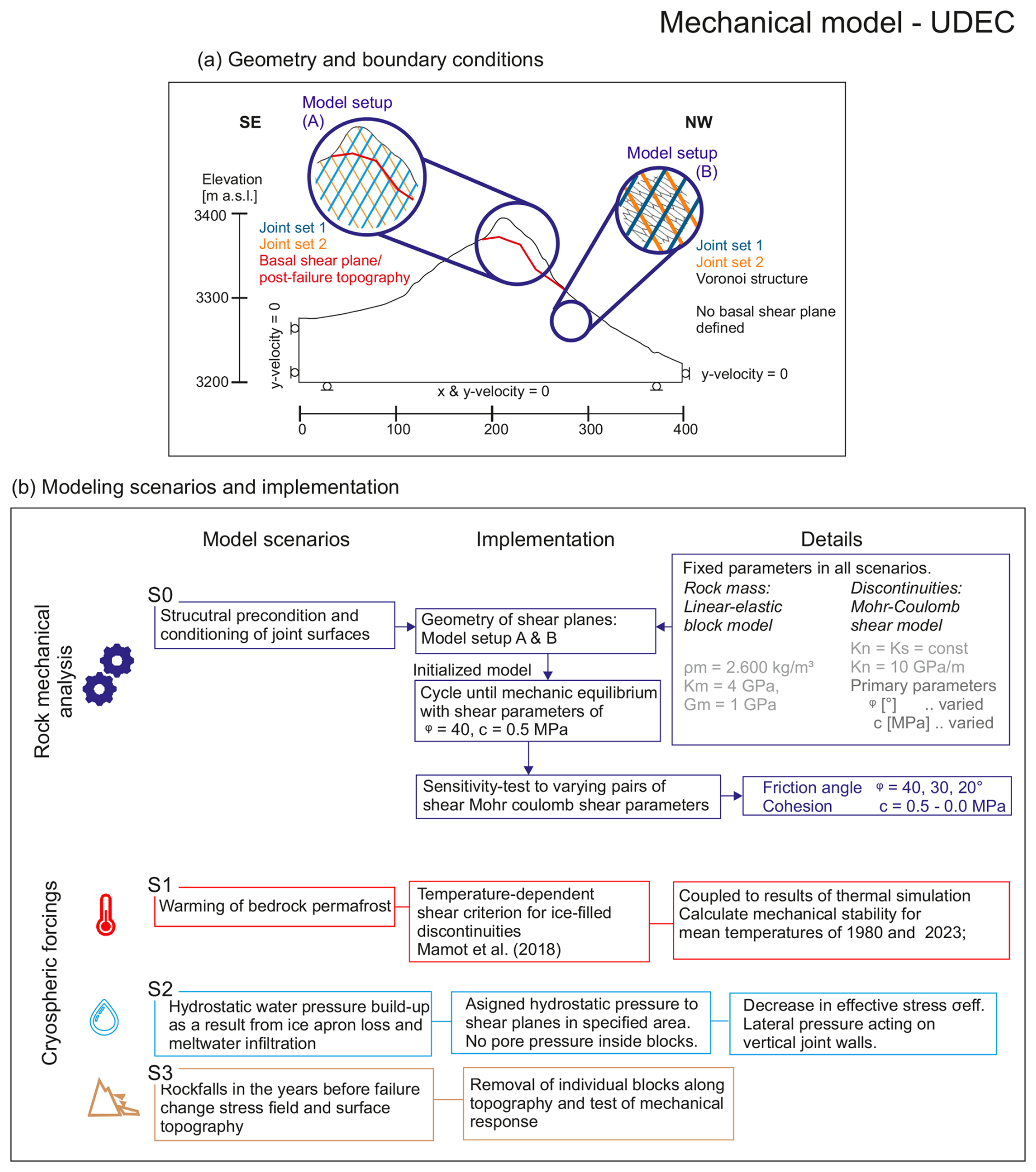
Figure 6 Simulation strategy for applying the mechanical modeling framework. (a) Model topography and boundary conditions, and two setups A & B varying in structural geometry, as shown in the circled overviews. Joint sets 1 and 2 are included throughout the full model domain. In setup A, the basal shear plane is sketched as a specified shear plane defining the structural failure path. In B, the basal shear plane is missing explicitly, but the model domain was added with a squeezed Voronoi structure, creating many possible failure paths. (b) Overview of the four modeling scenarios and their implementation.

3.2.3 Simulation strategy

We initialized a base model defining an in-situ stress ratio of k=0.5 ($\mathrm{0.5}{\mathit{\sigma }}_y={\mathit{\sigma }}_x={\mathit{\sigma }}_z$) prior to the simulation start (cf. Fischer et al., 2010; Rechberger and Zangerl, 2022), assigned shear parameters of ϕ=40° and c=0.5 MPa, and ran the simulation until reaching mechanical equilibrium. For all further scenarios simulated (Fig. 6b), this base model was used as the starting point. To assess stability, we cycled 30 000 model steps, studying overall model deformation and monitoring the displacement of specified locations within the rock mass throughout the simulation time.

3.2.4 Scenarios and implementation

In a first step, referred to as scenario S0, we tested the rock slopes' predisposition to failure by accounting for different structural model configurations (setup A & B) and back-calculated the rock slopes' hypothetical pre-failure condition by conducting a sensitivity test on varying pairs of shear parameters applied to all discontinuities throughout the model domain (i.e., analogous to Rechberger and Zangerl, 2022). The applied Mohr-Coulomb shear criterion relates shear stress τ [Pa] to normal stress σ [Pa] multiplied by the tangent of the friction angle ϕ [°] and adding cohesion c [Pa] as an intercept.

$$\begin{array}{}\text{(5)}& \mathit{\tau }=\mathit{\sigma }\cdot \tan \left(\mathit{\varphi }\right)+c,\mathit{\varphi }\in [\mathrm{20},\mathrm{40}]\mathit{°},c\in [\mathrm{0.0},\mathrm{0.5}]\mathrm{MPa}\end{array}$$

Based on considerations of possible promoting factors or triggers (Sect. 3.2.1, Fig. 5), we examine the following scenarios, aiming to investigate the mechanical response to a changing cryosphere. These scenarios represent quasi-static realizations of the rock slope under specific states or external forcings (Fig. 6b) and therefore illustrate mechanical system responses to isolated effects rather than complex interwoven system dynamics.

S1

Permafrost degradation

Discontinuities in permafrost rock are often filled with ice (Gruber and Haeberli, 2007; Krautblatter et al., 2013; Zangerl et al., 2019). The temperature of these ice-filled fractures or joints controls the shear strength of contact surfaces (Mamot et al., 2018, 2020; Huang et al., 2023a). To test the mechanical response to permafrost degradation, we performed a unidirectional thermo-mechanical simulation, where the output of the thermal model (CryoGrid 2D) was translated into the mechanical model (UDEC). We assigned temperature-dependent shear parameters ϕ(T),c(T) to discontinuities in the corresponding temperature regions resulting from the CryoGrid 2D simulation. Temperature zones from the CryoGrid 2D model output were replicated with regions in UDEC, whose discontinuities were assigned the corresponding temperature-dependent shear criterion. The herby used temperature-dependent Mohr-Coulomb shear criterion was derived from shear tests on rock-ice-rock sandwich samples and was proposed for ice-filled joints in permafrost rock by Mamot et al. (2018). In their equtation τ and σ are expressed in [kPa]:

$$\begin{array}{}\text{(6)}& \begin{array}{rl}\mathit{\tau }\left(T\right)=& \mathit{\sigma }\cdot \left(\right(\mathrm{0.42}\pm \mathrm{0.15})-(\mathrm{0.21}\pm \mathrm{0.06})\cdot T)\\ & +(\mathrm{53.3}\pm \mathrm{20.6}-(\mathrm{73.5}\pm \mathrm{8.8})\cdot T)\end{array}\end{array}$$

The equation incorporates temperature-independent (subscript _rock) and temperature-dependent (T) parts of the friction coefficient μ and cohesion c, which is demonstrated in a general form below:

$$\mathit{\tau }\left(T\right)=\mathit{\sigma }\cdot ({\mathit{\mu }}_{\mathrm{rock}}-\mathit{\mu }(T\left)\right)+(c_{\mathrm{rock}}-c(T\left)\right),$$

with μ=tan (ϕ).

The limit of applicability of the temperature-dependent shear criterion is given by the test settings in the laboratory, ranging from normal stresses between 100 and 400 kPa and temperatures between −8 and −0.5 °C. The ± sign reflects the spread of results stemming from the laboratory tests used to construct the shear criterion. In a simplified approach, we assume ice-filled discontinuities throughout the full model domain, while neglecting irregularities such as rock bridges or surface roughness of discontinuities.

S2

Transient buildup of hydrostatic pressure

The buildup of hydrostatic pressure within permafrost rock is a central trigger for releasing permafrost rock slope failure (Gruber and Haeberli, 2007; Fischer et al., 2010; Pfluger et al., 2025). Although observations and measurements of permafrost hydrogeology in rock slopes are scarce and typically site specific, a field study suggests plausible values for transient water columns in fracture systems of several decameters upon peak snow melt or rainwater infiltration periods (Scandroglio et al., 2025, back calculation from water discharge measured at fracture outlet). In addition, piezometric heads of more than 10 m were recorded in boreholes within fractured rock in permafrost (Offer et al., 2025), and sporadic permafrost (Aspaas et al., 2026). Moreover, failure scarps of larger failures often exhibit wet areas, observed directly after detachment, which point to locally ponded water within the rock mass short before sudden-failure conditions (i.e., Fluchthorn, Austria, 2023 event; Krautblatter et al., 2024; Piz Scerscen, Switzerland, 2024 event; PERMOS, 2024). With this scenario, we test the mechanical response to applied hydrostatic pressure equivalent to a 30 m water column, represting hydrogeological conditions upon peak surface water infiltration – compare to reported hydrostatic heads of 27±6 m during average snowmelt and 40±10 m for extreme events (Scandroglio et al., 2025). The pressurized zone is assigned a lateral width of 30 m and applied to different regions of the rock mass. Throughout the mechanical cycling, static water pressure is applied within discontinuities only, exerting normal stress on joint walls, while pore pressure within blocks is neglected. Temporal hydrogeological evolution is not explicitly modeled. Instead, spatially variable pressurized zones are used to represent conceptually inferred, locally ponded groundwater conditions within permafrost rock slopes, potentially promoted by channelized flow along fractures (Hasler et al., 2011; Magnin and Josnin, 2021). Unlike the analysis of observed rockfalls (Sect. 2) and permafrost warming (Sect. 3.1), changing groundwater conditions were not directly captured within the scope of this study, but their implications were inferred conceptually. This setup does not aim to reproduce actual groundwater flow conditions but isolates the mechanical effect of water pressure, emphasizing the sensitivity of slope stability to the spatial availability of water within the rock mass.

S3

Rockfalls and ice apron loss

Rockfalls or surface ice loss considerably alter the stress field of the rock slope in sudden moments or within relatively short periods, such as a decade (Deline et al., 2015). These processes have been found to substantially impact the morphology of Platteikogel rock slope before failure (Fig. 3g–i), and thus will be investigated in regard to mechanical response for preparing the detachment. Therefore, rock slope topography was altered by removing individual blocks, simulating the mechanical response adapting to the new stress field and topography.

Here, we apply the factor of safety (FoS) concept in a modified way. Traditionally, FoS quantifies slope stability by comparing resisting and driving forces (Wyllie and Mah, 2004). However, in our UDEC model with several thousand contact surfaces, this concept is challenging to adapt. As our focus lies on the final detachment phase, we interpret FoS through the evolution of displacement functions instead (cf. Pfluger et al., 2025). The amount of displacement may serve as a proxy to quantify failure. A displacement plateau towards the end of the simulation suggests that the rock slope remains stable approaching mechanical equilibrium (FoS > 1), whereas a continuously increasing displacement indicates progressive failure and the initiation of the detachment (FoS ≈ 1 or below).

4 Results

4.1 Thermal evolution of the subsurface

From 1980 to 2024, air temperature warming of ≈ 2 °C is evident at the location of Platteikogel (Fig. S8a). As permafrost in depths of several decameters evolves over decades, we display the mean annual temperature of mountain permafrost for the year 1980, at the start of the warming trend, and for 2023, shortly before the Platteikogel rock slope failure (Fig. 7a, b). Throughout this period, warming is evident within the full mountain and especially pronounced on the southeastern flank, while on the steep sections of the northwestern flank, low temperatures were better maintained. The temperature asymmetry mainly stems from the radiative warming of the sun-exposed bedrock, which is more pronounced for southeastern aspects, and is a result of the implemented temperature transfer function (Eq. 2). The vanishing ice aprons, which uncovered bedrock down to the elevation of the glacier surface at the southeastern flank between 1970 and 2000, controlled surface exposure and therefore enforced permafrost warming from the southeastern flank towards the northwestern flank. Comparing modeled temperatures along a 20 m deep monitoring profile running parallel to the rock topography, the simulations reveal mean annual temperatures below −3 °C, with a minimum of −5.5 °C modeled for the northwestern flank in 1980 (Fig. 7c). For 2023, only 15 % of the monitoring profile remained below −3 °C – marking the lense-shaped cold permafrost body at the northwestern flank – while at the southeastern flank temperatures warmed approximately to −2 °C (Fig. 7d). Table 2 displays modeled temperature and its increase at 20 m below the surface for specified locations. Overall, the modeled temperatures along the monitoring profile display a similar shape of temperature progression for 1980 and 2023, reflecting the impact of rising AT throughout the period. However, the ice apron loss on the southeastern flank, between a profile distance of 80 and 180 m, indicates a flip in temperature progression from a local depression (1980) towards a local peak (2023).

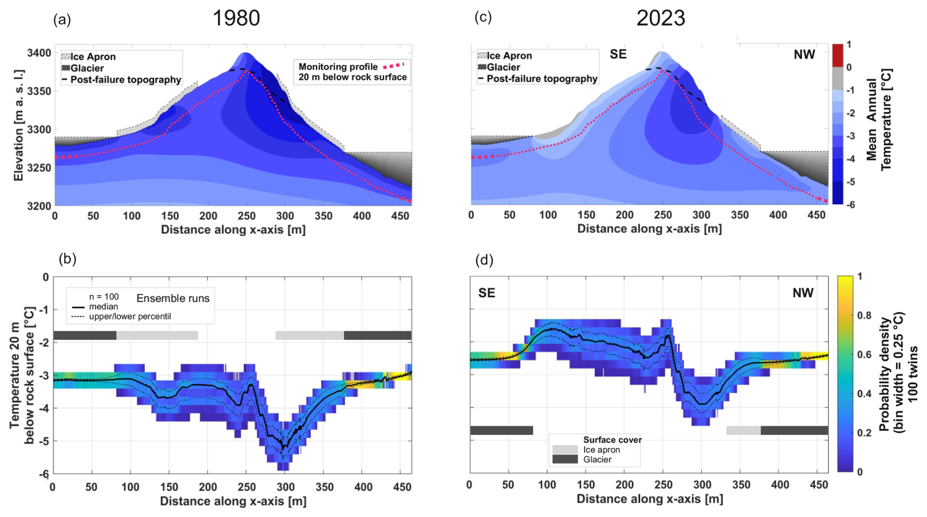
Figure 7 Modeled mean annual temperature distribution for (a) 1980 and (c) 2023. The glacier's location and ice apron extent are shown for reference. The plotted temperature distribution shows the median temperatures of all the simulated models (n=100). (b, d) Probability density plot of modeled temperatures shown at 20 m below the rock surface, accounting for parameter variations within the given ranges (Eqs. 1 to 4). Note: All models were run from 1900 onwards. The ice apron extent was fixed from 1900 to 1970, while the gradual top-down retreat was simulated from 1970 onwards.

Table 2 Modeled median annual permafrost temperatures at 20 m below surface picked from Fig. 7b,d for specified locations along the profile distance. Note that the vertical location above 150 m profile distance became ice-free in 1978, and above 300 m in 1987 (see Fig. S5).

^∗ ΔT (10 m) is given as an additional reference and not explicitly shown. Note that the difference of the 10-year-moving average air temperature between 1980 and 2020 is +2 °C.

To estimate the thermal impact of vanishing ice aprons, we compared a model with gradual ice apron retreat to a model assuming a fixed ice apron extent since 1970 onwards (Fig. 8). The observed retreat of ice aprons on the southeastern flank from 1970 to 2000, and its absence since 2000 onwards, indicates a surplus in permafrost temperature of ≈ 1 °C at 20 m depth in 2023. In contrast, retreat of the ice apron on the northwestern flank affected permafrost temperature only marginally, owing to the neglected radiative heating on the northwestern flank in our model.

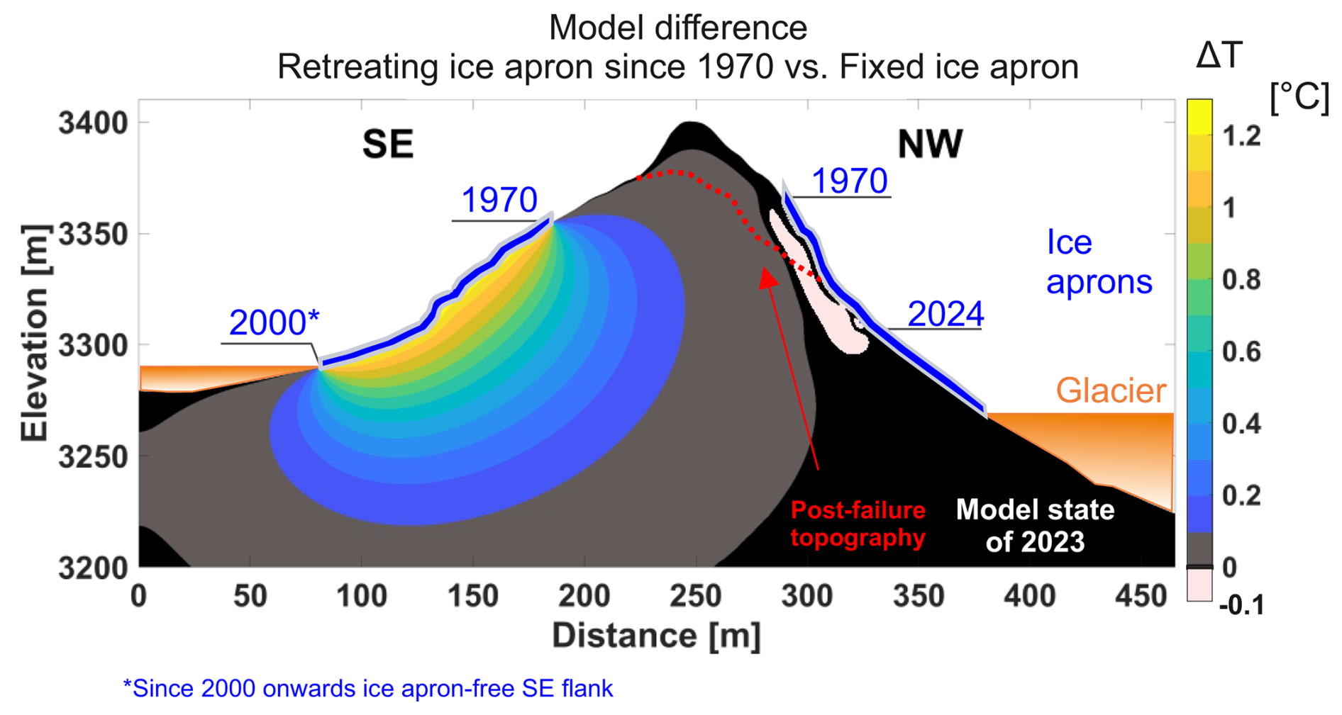
Figure 8 Impact of ice aprons on the evolution of mountain temperature. Difference in mean annual temperatures between a model assuming retreating ice aprons from 1970 onwards and a model assuming fixed ice apron extent from 1900 to 2023 according to the extent in 1970. Both models were forced since 1900 onwards, with implementing forcings calculated assuming the mean values specified in the defined ranges (Eqs. 1 to 4: (1) x=0, (2) SO_NW=0 °C & SO_SE=3 °C, (3) H_ice=5 m, (4) nF_glacier=0.5). Note: The SE flank indicates higher temperatures for absent ice aprons (radiative warming implemented with a +3 °C-air temperature offset for snow-free months only – Eq. 2). The NW flank indicates slightly lower temperatures as a result of the attenuated signal of AT (Eq. 3), and the assumed no-offset condition accounting for the absence of radiative warming at the NW flank. The black area in the model marks regions where $\left|\mathrm{\Delta }T\right|$ < 0.014 °C.

4.2 Mechanical investigations on failure processes

Mechanical simulations of setups A and B yielded similar results despite differences in structural detail (explicit basal shear plane vs. implicit shear plane developing along multiple substructures). In the following, we concentrate on setup A, displaying results for scenarios S0 to S3, while presenting results of setup B in the appendix (Figs. A3–A6). We briefly address the differences between setups A and B at the end of this section.

4.2.1 Model with basal shear plane – explicit failure path – setup A

S0

In order to back-calculate the theoretical pre-failure conditions of critical discontinuities short before the detachment, we ran sensitivity tests of varying shear parameters, which revealed the following situation (Fig. 9a): Of the conducted 21 simulations, 9 resulted in horizontal displacement of the tracked block of more than 0.01 m (Fig. 9d). While models with ϕ = 40° remained in stable conditions, indicated by the displacement functions approaching a plateau at the end of cycling, models with ϕ = 30 or 20° and cohesion below 0.1 or 0.2 MPa, respectively, display continuously propagating displacement at the end of cycling. The full activation of the basal shear plane is presented in the sequence of Fig. 9b–d, where Fig. 9b first indicates activation of the central discontinuity set. Assuming a reduction in cohesion, i.e., through progressive weathering or rock fatigue, in Fig. 9c, the shear plane is activated starting from the rock slope's toe and from there extending towards deeper regions. In Fig. 9d, the full shear plane is activated, and the displaced blocks do not regain stable positions.

S1

Assuming the presence of ice-filled discontinuities and their temperature-dependent shear strength according to the permafrost temperature short before the detachment (Fig. 10a), the simulation revealed stable slope conditions (Fig. 10b). In scenario S0, failure occurs as a result of progressive destabilization of the rock slope's toe. These kinematics were prevented here, as permafrost temperature is lowest and shear parameters are highest at the steeper parts of the northwestern flank. In contrast, warmer temperatures and lower shear strength dominate the mechanically less relevant southeastern flank. It is worth noting that even a more pessimistic perspective, with higher temperatures simulated (approx. +1 °C compared to the 2023 median temperature state shown in Fig. 7c) and incorporating the lower bound of spread from the conversion of temperature-dependent shear parameters (Eq. 6, lower values of shear parameters), results in stable rock slope conditions.

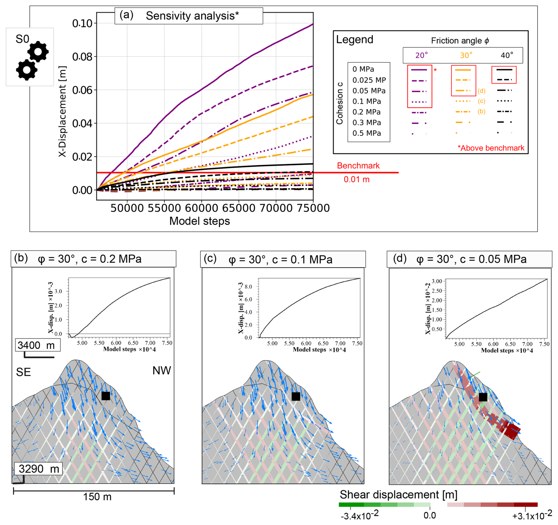
Figure 9 Rock mechanical back analysis characterizing pre-failure contact surfaces (scenario S0,A) – Results of the UDEC simulation. (a) Compilation of sensitivity tests and the corresponding displacement functions for the location of the black square shown in panels (b)–(d). Note that displacements from the initialization of the model were excluded from the graph. (b–d) Exhibiting model states after cycling 30 000 model steps in the order of a gradual decrease in cohesion. The coloured patches indicate the absolute shear displacement along the contact surfaces of blocks at the end of cycling (dual-coded with the size to display the most prominent areas of shearing within the model). Blue vectors mark the displacement direction and relative magnitude. The black square marks the location of the monitoring point, while the graph on top shows the displacement in the horizontal direction along mechanical cycling time. For intercomparison, panels (b)–(d) share the same scale for shear displacement.

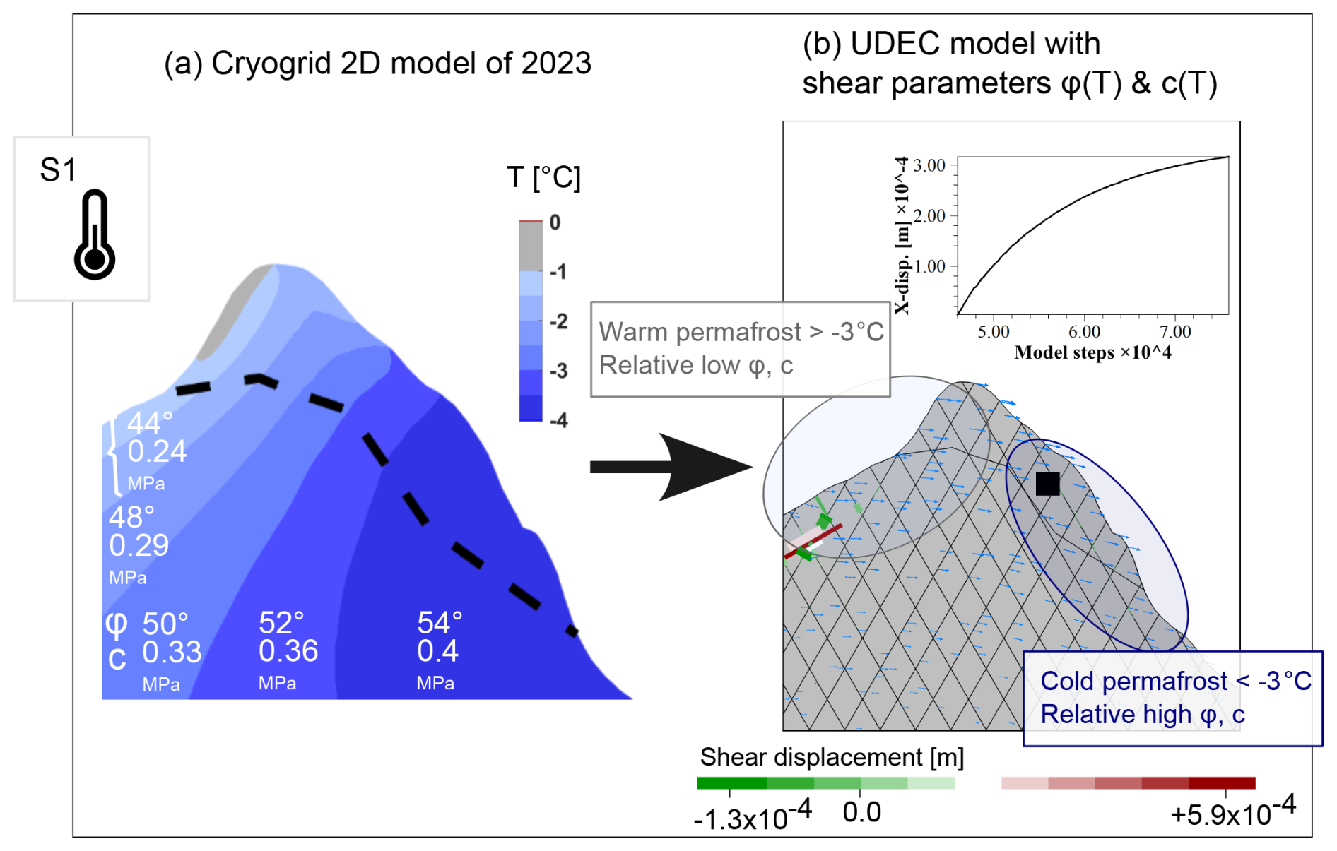
Figure 10 Coupling of the temperature-dependent shear criterion to the thermal model state (scenario S1,A). (a) Displaying thermal model state of 2023 as calculated with Cryogrid (Fig. 7c) and corresponding temperature-dependent shear parameters for ice-filled discontinuities acc. to Eq. (6), mean values used. (b) UDEC results of the unidirectional coupled model at the end of cycling. Explanation of the chart as shown in Fig. 9.

To test the mechanical response to hydrostatic pressure or rockfalls (scenarios S2 and S3), we use the simulated results from the models of scenario S0 (the back-calculated pre-failure state, with a factor of safety (FoS) slightly above 1, i.e., ϕ=30° and c = 0.1 MPa, as shown in Fig. 9) and of scenario S1, which represents the temperature-dependent shear model according to 2023 temperatures (Fig. 10b), as the basis.

Base model S0 – Pre-failure conditions ϕ=30° and c = 0.1 MPa

S2_S0

Applied hydrostatic pressure leads to varying magnitudes of shear displacement, mainly depending on where the pressure acts in regard to the monitoring location (Fig. 11a–c). For the defined hydrostatic pressure, the displacement functions of the models (Fig. 11a–c) do not approach a plateau, indicating unstable slope conditions. In Fig. 11a, b, the basal shear plane is fully activated. In Fig. 11c, the basal shear plane is partly activated, only in the areas at the toe of the rock slope. Yet, if that region detaches, the stress is redistributed to other parts at the basal shear plane above, gradually shaping a failure path which evolves towards the peak of the mountain, similar to what is demonstrated in Fig. 9b–d with the gradual decrease in cohesion.

S3_S0

Rockfalls affect the stress field and change the local topography. The removal of a block at the lower slope part results in an increase in x-displacement, as indicated in the displacement function. Yet the form of function appears to approach a plateau, indicating the model is likely to regain equilibrium (Fig. 11d). For the removal of blocks at the upper part (Fig. 11e), the model exhibits an elastic response (see displacement function), suggesting the overall model kinematics were governed by the base model S0, which was used as input. Through local unloading, less stress was exerted on the steeper section of the basal shear plane, stopping the ongoing gradual deformation (compare the displacement function at S0 vs. S3).

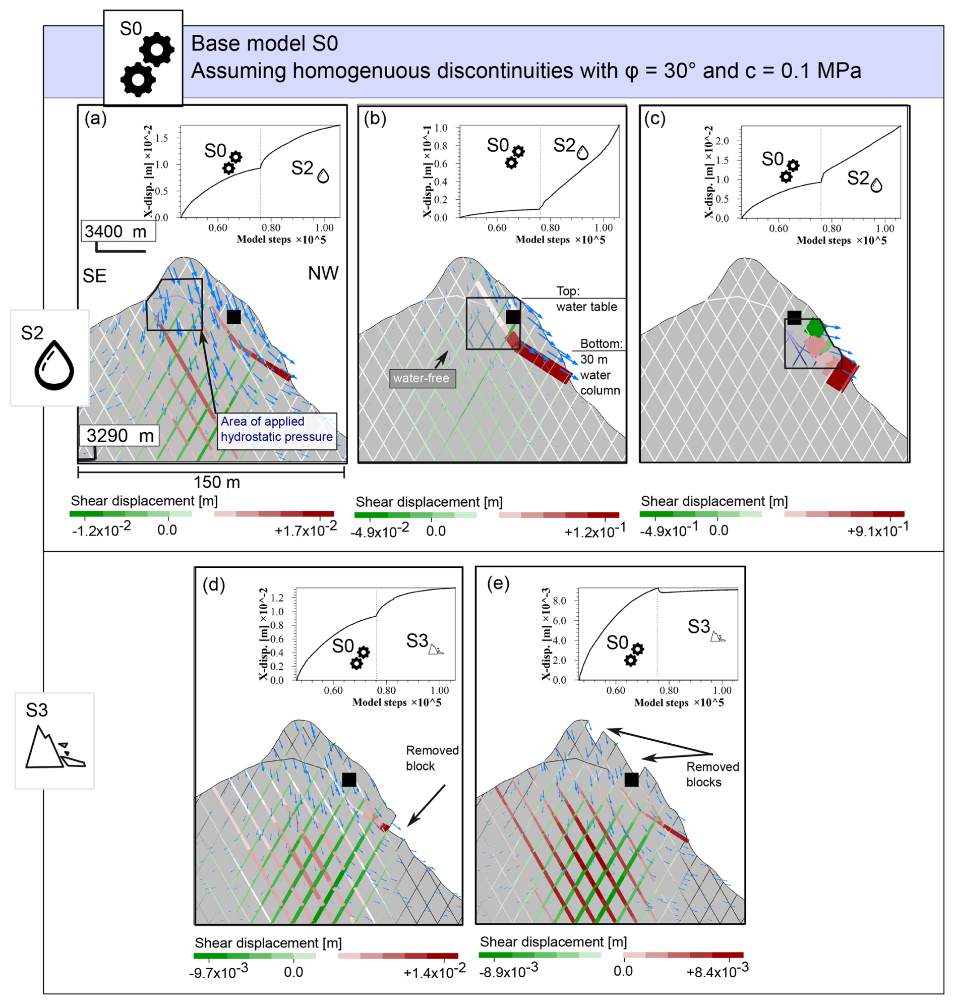
Figure 11 The impact of hydrostatic pressure and rockfalls on rock slope stability calculated with UDEC for model setup A using the model of back-calculated pre-failure state from scenario S0 (ϕ = 30° and c = 0.1 MPa; see Fig. 10c) as a basis. (a–c) Impact of hydrostatic water pressure on slope mechanics, illustrated for three different locations of assumed water pressure. (d, e) Impact of rockfalls (removal of individual blocks) on slope mechanics. Explanation of charts as shown in Fig. 9. Note that the state of the model is displayed for the end of the simulation, and the illustrated shear displacement shows the cumulative displacement of S0 and S2 or S3, respectively.

Base model S1 – Temperature-dependent shear model of 2023 temperatures

S2_S1

Applied hydrostatic pressure leads to a relatively distinct increase in shear displacement (Fig. 12a–c). However, activated shear planes are isolated within the rock mass, leaving the entire basal shear plane largely unaffected. Hydrostatic pressure exerted in the area of the southeastern or northeastern flank (Fig. 12a, c) shows how the uppermost blocks become unstable and detach from the rock slope – simulating a local rockfall release rather than the major release. Hydrostatic pressure exerted at a centered position within the mountain (Fig. 12b) shows the modeled highest displacement according to the displacement function. Yet, this is a local effect as the monitor point lies within the area of applied water pressure, while the basal shear zone at its margins remains unaffected.

S3_S1

The effect of a rockfall in the area of the slope's toe, i.e., the removal of a block (Fig. 12d), shows a direct response by the activation of shearing along contacts of neighboring blocks, but leaves regions more distant unaffected. In contrast to the base model S0, block removal in the upper slope (Fig. 12e) reveals an elastic stress-relief response (blue arrows), enhancing local shear activation at shallow discontinuities above the basal shear plane.

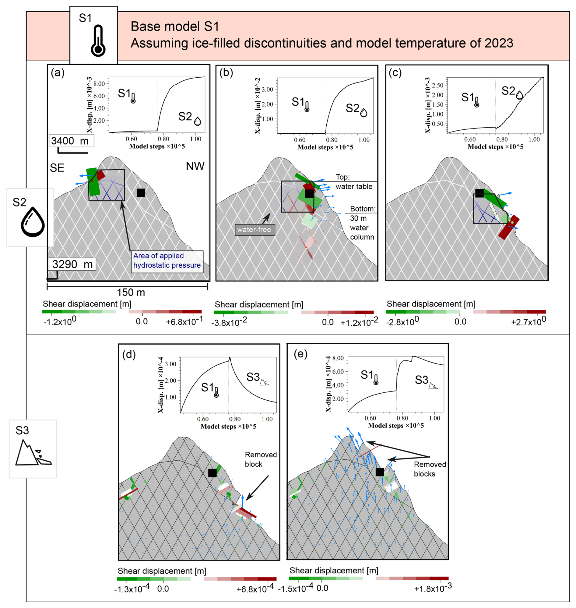
Figure 12 The impact of hydrostatic pressure and rockfalls on rock slope stability calculated with UDEC for model setup A using the model with the temperature-dependent shear criterion S1 acc. to 2023 (Fig. 10b) as a basis. (a–c) Impact of hydrostatic water pressure on slope mechanics, illustrated for three different locations of assumed water pressure. (d, e) Impact of rockfalls (removal of individual blocks) on slope mechanics. Explanation of charts as shown in Fig. 9. Note that the state of the model is displayed for the end of the simulation, and the illustrated shear displacement shows the cumulative displacement of S1 and S2 or S3, respectively.

4.2.2 Model with multiple shear planes – implicit failure path – setup B

S0

Comparing the results of the structural model setup A (defined basal shear plane) with B (Voronoi structures, without explicitly defined shear plane, but higher degree of structural detail), we briefly describe the difference. For the back-calculation of the pre-failure state of discontinuities (scenario S0), both setups reveal the same parameter combinations that exceed the 0.01 m displacement benchmark, except ϕ=40° & c=0.025 MPa, which reaches 0.009 m (Fig. A3a). Simulated displacement magnitudes resemble both setups (Fig. A3b–d), yet due to the many substructures, shearing occurs along many discontinuities rather than one central structure. The rock slope failure under setup B was formed by multiple parallel shear planes, which are slightly below the pre-defined basal shear plane in setup A. Despite the implicit approach with the Voronoi structures, almost the same failure volume could be replicated (Fig. A3d).

S1

The coupled temperature-dependent shear criterion demonstrates marginal shear displacement on the order of 10⁻⁴ m for 2023 temperature, which is in the same magnitude range as shown for setup A. Shear displacements in critical regions are not observed, while localized marginal shearing areas originate within deeper areas (Fig. A4).

S2

Applied hydrostatic pressure demonstrates a distinct impact on overall shear displacement for base model S0 with back-calculated pre-failure shear parameters (Fig. A5a–c), similar to setup A. The model state according to the temperature-dependent shear criterion of 2023 (S1) was less affected, showing a similar model response as in setup A (Fig. A6a–c).

S3

Rockfalls affecting the slope topography and the stress redistribution led to enhanced displacement of the failure volume at setup B, for both locations of rockfalls simulated (base model S0, Fig.A5d, e). In contrast to setup A, where shearing decreases as a result of rockfalls from the ridge area (Fig.11e), the rockfall from the same area indicated the opposite effect for setup B, with enhanced shearing at similar areas. Regarding the base model S1, both setups A and B resulted in similar model responses (cf. Figs.12 & A6d, e).

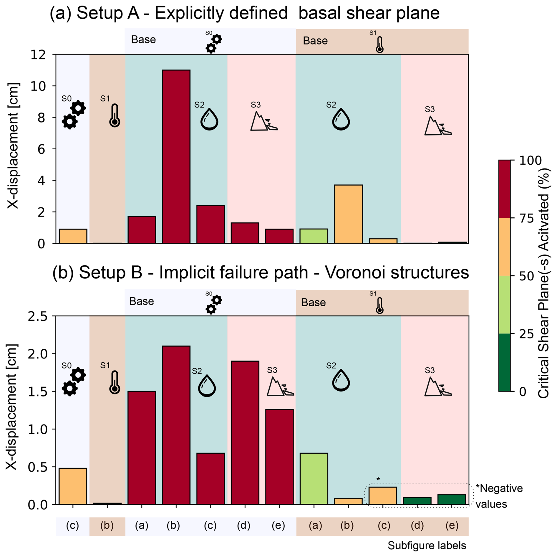
Figure 13 Compilation of results listed for each scenario shown for the structural model configuration of (a) setup A and (b) setup B. The bars display the absolute x-displacement at the end of cycling 30,000 model steps for the location of the monitoring point shown in the reference figures. Results stem from individual simulations shown for panel (a) in Figs. 9–12 and for panel (b) in Figs. A3–A6. The color scale indicates the relative share of the basal shear plane/critical shear planes that is activated at this model state. Note: In UDEC, “model steps” refer to numerical iterations. One model step corresponds to 0.000492 s (setup A) and 0.000342 s (setup B) of physical time, regardless of the scenarios simulated. Model steps scale linearly with time.

To quantify the mechanical impact of the individual processes, we directly compare scenario results by using the modeled absolute x-displacement recorded at the end of cycling 30 000 model steps for the specified monitoring location as the benchmark metric (see displacement functions in the figures). The comparison in Fig. 13 demonstrates that hydrostatic pressure (as modeled here) had the most pronounced impact on the kinematic response of the rock slope. Permafrost, as modeled with the implementation of the temperature-dependent shear criterion, had a minor impact on the destabilization process. The impact of rockfalls depends on the structural model setup: While setup A showed minor effects, setup B exhibited x-displacements comparable to those suggested by hydrostatic pressure (cf. S3 in Fig. 13). Small block sizes facilitated shearing along many substructures and locally favored the sliding of neighboring blocks affected by the void at the post-rockfall state. In general, a smaller block size (setup B) led to lower total x-displacement at the monitoring location, compared to a larger block model with a defined shear basal shear plane (setup A). Within a single setup, however, displacement patterns remain internally consistent and comparable between scenarios. Both model setups indicate that at higher pre-failure shear strength (base model S1), the kinematic rock slope response is less susceptible to hydrostatic pressure applied and rockfalls.

5 Discussion

5.1 Does ice apron loss promote the Platteikogel rock slope failure?

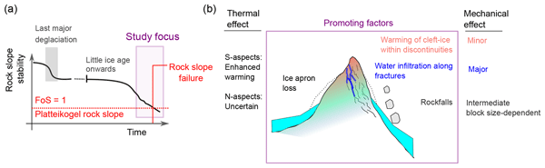
The Platteikogel rock slope failure originated in heavily weathered gneiss with closely spaced foliation and joints in steep terrain, providing favorable preconditions for gravitational mass movements (Fischer et al., 2006). To discuss the mechanism leading to the detachment, we distinguish between promoting drivers which act on a rock slope system over months to millions of years (Dietze et al., 2017), preparing the rock slope system towards future failure (Prager et al., 2008), and trigger referring to an event which directly leads to the main detachment in sec, min, hours, or days after the event – i.e., rainfall or seismic shaking (Leinauer et al., 2024). The patterns shifting a rock slope system towards instability are typically determined by nonlinear key controls in space and time (Krautblatter and Moore, 2014). While we did not identify a clear trigger for the Platteikogel rock slope failure, we observed processes like ice apron loss over 50 years. The loss of ice aprons and their impact on permafrost, hydrogeology, and rockfall processes (Fig. 5), illustrates how multiple drivers interact during the transition from paraglacial to periglacial conditions, highlighting the nonlinear influence on rock instability.

The destabilizing effect of permafrost degradation on rock slopes has been cross-confirmed by various methods: Laboratory tests simulating permafrost degradation underpin the change of physical rock (Mellor, 1973; Dwivedi et al., 2000; Davies et al., 2001; Krautblatter and Hauck, 2007; Draebing and Krautblatter, 2012) and mixed rock-ice material properties (Mamot et al., 2021; Han et al., 2023; Huang et al., 2023b). Field studies demonstrate that observed kinematics and permafrost dynamics are strongly interwoven, impacting small-scale objects such as rock pillars (Weber et al., 2025, volumne 100 m³), and full rock slope systems on the slope-scale (Etzelmüller et al., 2022). Dated prehistoric slip surfaces suggest that rock slide formation coincided with permafrost degradation phases, leading Hilger et al. (2021) to conclude that permafrost degradation was likely the primary driver for the failure of the studied post-glacial rock slides. Moreover, empirical evidence confirms enhanced geomorphological activity during the paraglacial transition, from small-scale rockfalls (Hartmeyer et al., 2020; Draebing and Mayer, 2021) to large-scale rock slope failures (Gruber and Haeberli, 2007; Ballantyne et al., 2014; McColl and Draebing, 2019). Whether rock slopes can withstand this transition depends on their pre-failure condition – that is, whether their overall factor of safety was already close to failure.

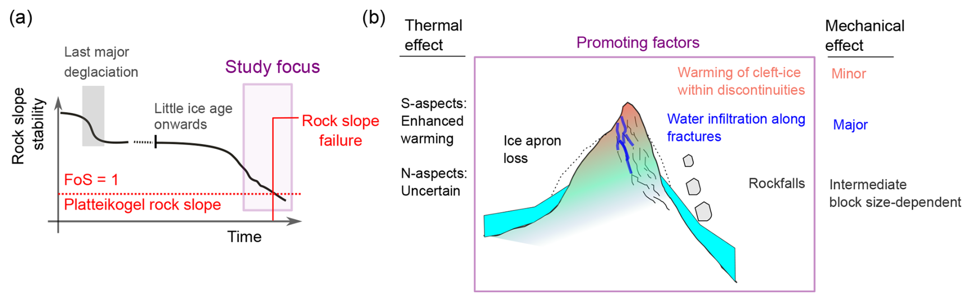
Figure 14 (a) Conceptually inferred stability function of the Platteikogel rock slope, highlighting the non-linear influence during the peri-paraglacial transition. (b) Dominant promoting factors investigated in this study that are relevant in the period shortly before failure. Results from the thermal and mechanical simulations are included to illustrate the corresponding impact.

The concept of progressive failure mechanism and the promotion of the Platteikogel rock slope failure is explained theoretically (Fig. 14a) and on the basis of our simulation results (Fig. 14b): Cold permafrost since the Little Ice Age stabilizes the slope by adding cohesion through ice in fractures, and suppressing crack propagation (Krautblatter and Leith, 2015). However, in recent decades, ice apron loss and warming air temperatures have accelerated permafrost warming. The observed rockfall activity, together with ice apron loss, modified the topography. Consequently, elastic rock mass adaptation leads to widening of joints (Leith et al., 2014; Grämiger et al., 2017). Ice apron loss, joint widening, and heterogeneous permafrost conditions, which are typically found in complex topographic terrain (Noetzli et al., 2007), favour the infiltration of water into the rock slope and therefore potentially enable hydrostatic pressure buildup within stability-relevant areas (scenario S2). Given sufficient accumulated pre-failure damage (i.e., base model S0), the rock slope is prone to failure upon hydrostatic pressure buildup during peak water infiltration events (snowmelt/rainfall event, S2) or as a response to rockfalls (S3, setup B: small block-size model). Yet, shear strength degradation as a result of permafrost warming (S1) had a minor impact on the destabilization (Fig. 14b). The implications of permafrost warming and strength degradation are discussed in the following section in detail.

5.2 Beyond thermal warming: Superimposed processes accelerate failure

The coupling of the temperature-dependent shear criterion for ice-filled discontinuities to modeled permafrost temperatures of 2023 (Scenario S1, Fig. 10) reveals stable slope conditions for the Platteikogel rock slope, suggesting that the degradation of shear strength of ice-filled discontinuities through warming temperatures alone can not explain the release of the observed rock detachment. Therefore, we draw the following conclusions.

1. Other mechanisms superimpose to promote slope failure – i.e., hydrostatic pressure as described by (Gruber and Haeberli, 2007; Cathala et al., 2024; Pfluger et al., 2025) and/or the effects of mass unloading and topographic modification (through glacier ice retreat; Fischer et al., 2010; Leith et al., 2014), which in the case of Platteikogel, is explored through rockfalls or ice apron loss. With the mechanical modeling study, we could demonstrate the effect of both process, while the impact on the destabilization, here measured in terms of shear displacement – was greater for a model which had accumulated more fatigue and was closer to a state of sudden-failure (= rock detachment, scenario S0), than for a model suggesting less pre-failure damage (S1, compare Figs. 11 & 12). The difference in shear parameters suggests that the temperature-dependent shear criterion used in S1 potentially overestimates the actual pre-failure shear strength (${\mathrm{\Delta }}_{\mathrm{S}\mathrm{1}-\mathrm{S}\mathrm{0}}\mathit{\varphi }>+\mathrm{14}\mathit{°}$, ${\mathrm{\Delta }}_{\mathrm{S}\mathrm{1}-\mathrm{S}\mathrm{0}}c>+\mathrm{0.14}$ MPa). The modeling results indicate that in the case of scenario S0, the imposed factors may act as a trigger for the major detachment, while in scenario S1, they may lead to the accumulation of rock mass damage, promoting failure in the future.

2. The discontinuity surfaces are heterogeneous and more complex in nature. Yet, the presence of ice-filled discontinuities according to (Eq. 5; Mamot et al., 2018) was prescribed troughout the full model domain in scenario S1, assuming similar shear charaterisitcs under same temperature. The applied temperature-dependent shear criterion explains the final stage of shear failure along ice-filled contact surfaces of rocks, given that rock bridges are eroded, asperities are smoothened, and shear strength is controlled only by the compound material of ice and rock. It accounts for failure timing linked to temperature, where cold delays failure. Given the theoretical pre-failure conditions, as created in the laboratory for tested rock–ice–rock sandwich samples with diameters of 15 cm and artificially smoothed rock surfaces, warming above −1 °C would lead to the rock slope failure, assuming a model with uniform temperatures. Compared to the simulated heterogeneous temperatures, with average permafrost temperatures of ≈ −3 °C at stability-relevant areas at the rock slopes' toe (Fig. 7d), this corresponds to a temperature discrepancy of more than 2 °C. In any case, extrapolating the laboratory constraint conditions of ice-filled contact surfaces to a natural shear plane spanning 100 m in length is a strong simplification, neglecting other shear plane features and irregularities. For intact rock, serving as a proxy for rock bridges, a model explicitly capturing temperature-dependent shear strength degradation in the range from −5 to 0 °C has not yet been established. Nevertheless, existing studies clearly indicate that rock mechanical properties are sensitive to warming at these temperatures, demonstrating a general warming-related weakening (see Sect. 5.1).

Although our thermo-mechanical modelling approach involves several uncertainties (see supplementary Discussion – Sect. S3 in the Supplement), it provides a first-order assessment of the central processes that promote permafrost rock slope failures (cf. Gruber and Haeberli, 2007; Krautblatter et al., 2013; Grämiger et al., 2020).

The mechanical model indicates that the failure is strongly controlled by the stability of the toe of the slope. Simulated rockfalls (scenario S3) yield in attidional displacement of the failed rock mass above – especially for the model with small block sizes (setup B) and a shear parametrization close to failure (Fig. A5d, e). These findings suggest that the Platteikogel rock slope failure could have occurred as a rock collapse (sequential smaller detachments). However, morphological observations suggest that detachment happened as one major, single push event. The form of deposits (bifurcation – see Fig. 2a, e), the reach angle of 24.6°, and $H/L$ ratio of 0.45 suggest that the failure can kinematically be classified as a rock avalanche, likely resulting from a single push event (cf. kinematic model in Fig. S6). The runout length can be explained by the low contact friction and lubrication effect (basal water film) resulting from the basal contact to the glacier surface and present snow cover. The failed volume of 50 000 m³ is at the lower end of cubatures reported for rock avalanches (cf. rock collapse vs. rock avalanche in Hermanns et al., 2022). To conclude, the Platteikogel rock slope failure likely occurred as one major failure event, which was preceded by rockfalls observed in the decade before (Fig. 3) and by detachments shortly after. Post-failure activity was indicated by proximal deposits that are generally larger than distal deposits (Detailed map in Fig. S7), suggesting secondary failure events.

5.3 Ice apron loss likely enhances thermal and hydrogeological changes

Ice aprons represent a glacial heritage, often preserving ice several thousand years old (Guillet et al., 2021). Their existence indicates the presence of permafrost underneath (Benn and Evans, 2014). The observed area decline in the Western Alps in the last decades (Guillet and Ravanel, 2020; Kaushik et al., 2022; Ravanel et al., 2023) was also evident at the Vernagtferner Basin in general (compare time series of historic orthophotos; Table A1, ii), which is located in the Eastern Alps of Europe, and in detail in direct proximity to the Platteikogel detachment area (Fig. 3a–c).

The observed ice apron loss at Vernagtferner, including the Platteikogel site, is primarily attributed to continuously rising air temperatures since 1980 (Fig. S8a). Winter precipitation has remained largely stable since 1970, with no significant trend (winter mass balance of Vernagtferner used as proxy; Fig. S8b). In contrast, summer precipitation has increased since 1980, with the trend intensifying after 2010 (10-year moving average: 500 mm in 1980, 650 mm in 2010, and 800 mm in 2020; Fig. S8c). However, it remains unclear and largely site-specific if ice aprons respond to a general increase in precipitation by growth or thickness loss. Yet, for the case of Platteikogel, the pronounced area loss of ice apron at the southern flank occurred before 2000, suggesting a strong control by rising air temperatures.

In our thermal model, ice aprons were represented as static bodies with temporally varying extents, forced by linear retreat rates inferred from orthophotos. This approach did not capture their dynamic interaction with atmospheric variables. Current knowledge on ice aprons remains limited, with scarce temperature data for the ice or underlying rock (Ravanel et al., 2023), and no information on heat fluxes between the rock, ice, and atmosphere. To approximate the thermal characteristics of ice aprons in our thermal model, we applied a low-pass filter on air temperatures mimicking buffered seasonal signals with ice apron thickness (Eq. 3). This reproduced the general pattern observed in temperature profiles of glacier ice with depth (Jacquemart et al., 2025) and incorporated the elimination of clear seasonal signals beyond 10 m depth.

Our model highlights the thermal contrast between previously ice-covered and now ice-free rock surfaces, which have since been exposed to radiative warming (Fig. 8). The results clearly demonstrate the impact on surfaces receiving high amounts of solar radiation, whereas for northwest-facing rock slopes, the effect is less pronounced and cannot be reliably assessed with given information and no constraints on rock–ice–atmosphere heat fluxes.

With these abstractions of ice aprons, we capture only part of the cryospheric dynamics. Rather than reproducing full system complexity, we demonstrate how ice apron loss can influence permafrost degradation over multiple decades through conductive processes and simplified atmospheric coupling, while neglecting precipitation and snow dynamics. The conceptual model of ice aprons (Fig. 5), illustrating interactions with the hydro- (Francese et al., 2025; Pfluger et al., 2025) and geosphere (Hartmeyer et al., 2020; Fey et al., 2025) concomitant with atmospheric warming, builds on empirical relationships and inferred processes from studies conducted on glaciers. Due to similarities and the scarce knowledge about ice aprons, analogies were drawn between glaciers and ice aprons. For the Platteikogel rock slope failure, the modeled ice aprons did not thermally affect the mechanically critical shear planes. However, the ongoing rockfall activity and hydrogeological changes are likely associated with the retreat of ice aprons.

6 Conclusion

The 2024 Platteikogel rock slope failure (Vernagtferner Basin, Austria) provides a benchmark case demonstrating how ice apron loss and permafrost warming promote the failure of high-alpine rock slopes. Multi-decadal ice apron area loss and pre-failure rockfall activity preceded the studied major rock detachment. Based on field observations and conceptual reasoning, we developed a numerical modeling study drawing the following conclusions:

• Climate warming is the main driver for rising permafrost temperatures between 1980 and 2023. Conductive thermal simulations indicate decadal warming at 20 m depth before rock detachment: +0.14 °C per decade below the cold-based glacier in the area of the bergschrund, +0.37 °C per decade below the ridge top at the location of the basal shear plane, +0.47 °C per decade at the southeast-, and +0.33 °C per decade at the northwest-exposed, ice-apron free slopes (median values of 100 twin simulations).

• Ice apron loss accelerates permafrost warming through atmospheric exposure of rock surfaces, as shown by conductive thermal modeling. Forced with a monthly air temperature offset for solar radiative warming of +3 °C for southeast-exposed slopes during snow-free months, the model suggests that the observed loss of the ice aprons on the southeastern flank between 1970 and 2000 caused approximately 1 °C of additional permafrost warming at 20 m depth by 2023, relative to simulations where the ice aprons remained intact from 1970 to 2023. With radiative warming as the dominant factor in warming rock upon becoming ice-free, the effect is less pronounced for aspects with little incoming radiation.

• Modeled mean 2023 temperatures along the basal shear plane (−4 to −2 °C) indicate stable slope conditions, as supported by the mechanical model coupled to the thermal simulation. Herby, we linked the shear strength, as the dominant parameter of rock slide control, to a temperature-dependent shear model, valid for ice-filled discontinuities. The finding suggests that other mechanisms apart from permafrost warming acted in driving the observed rock detachment, the slope did not fail along ice-filled discontinuities, or the application of laboratory-derived temperature-dependent shear parameters does not match real-world shear surface conditions.

• Degrading ice aprons feature geomorphic change by enhancing frost-weathering activity through atmospheric recoupling and by enabling water infiltration into rock slopes, which in turn facilitates the generation of rock slope failures. Stress alterations from ice apron loss and rockfalls, as well as hydrostatic pressure buildup, drive progressive rock slope failure, as demonstrated by the mechanical simulation.

• Given the major ice apron loss and structural predisposition at the Platteikogel, similar rock slope failures may be anticipated if kinematic monitoring data are available. However, precise failure time predictions without kinematic data remain unrealistic.

Appendix A

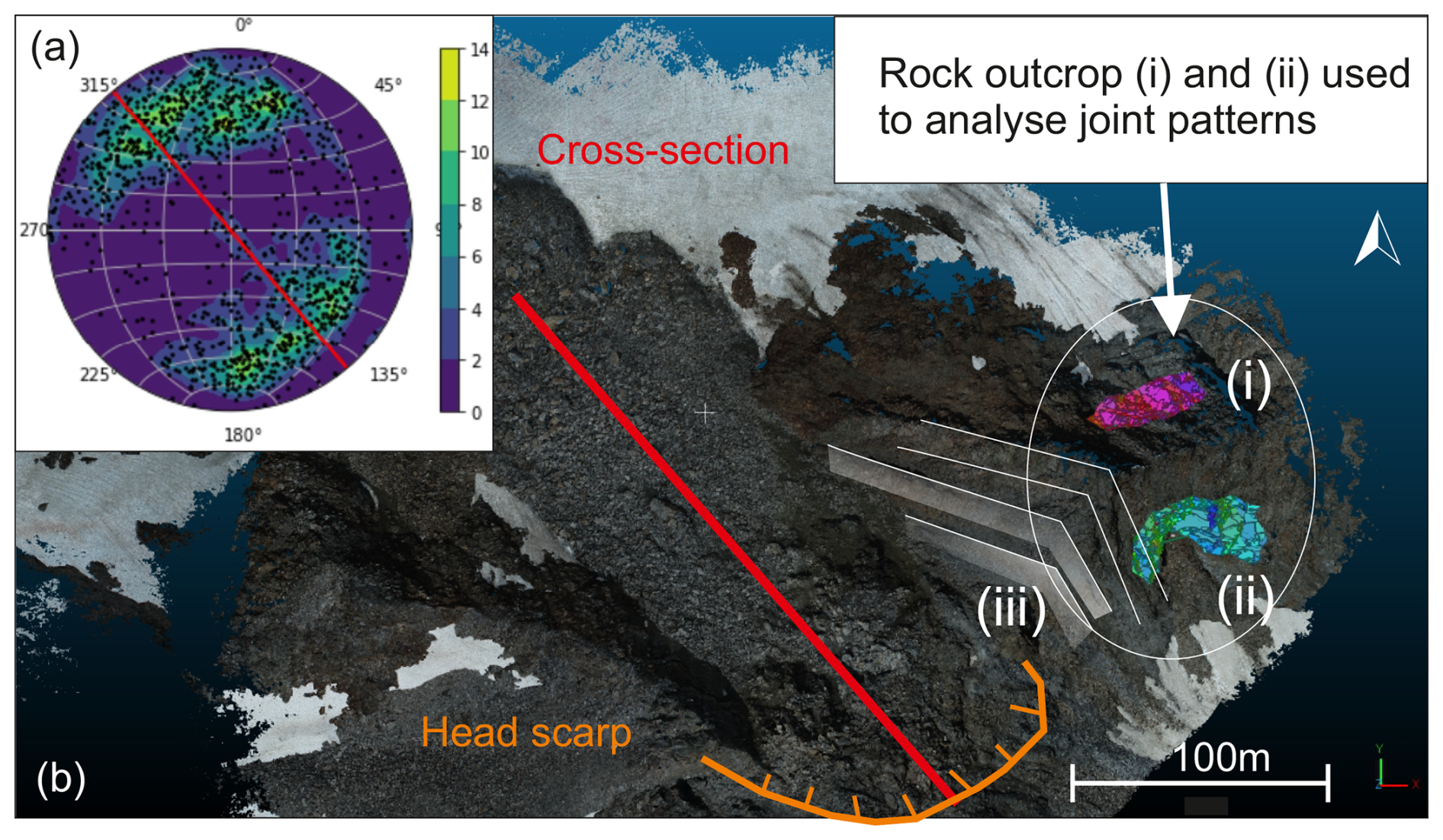
Figure A1 Structural analysis of two rock outcrops in proximity to the detachment area. In total, 11 339 planes were reconstructed and analyzed using the FACET plugin in Cloud Compare software (Dewez et al., 2016). Parameters for FACET plugin: Fusion algorithm Kd-tree, max-anlge 20, max relative distance 1.00. (a) Stereographic projection of the geological planes using CLAR-method for illustration and “Kamb exponential smoothing”: Units are in numbers of standard deviations by which the density estimate differs from uniform (produced with mplstereonet; Kington, 2024). The two identified clusters are joint planes. (b) Orthophotographic view of the ridge exhibiting the detachment area of the rock slope failure, including the location of the two rock outcrops and the whitish highlighted structural features of morphology (iii) that intersect the ridge: Steep dipping, perpendicular oriented foliation planes. The UAV point cloud model recorded in August 2024 was used as the basis for analysis in Cloud Compare (2 cm model resolution).

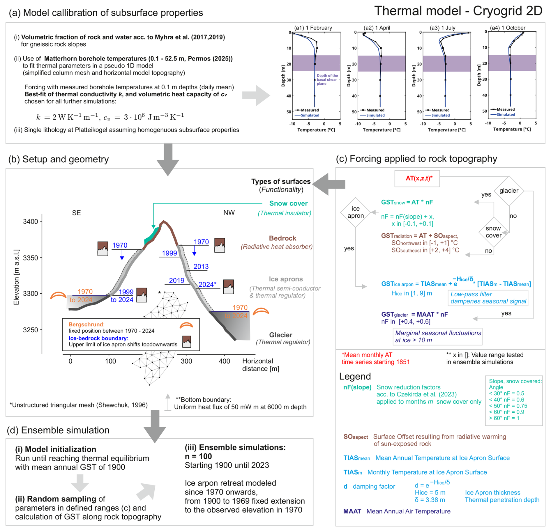
Figure A2 Simulation strategy applying the permafrost model Cryogrid 2D: (a) Calibration of thermal parameters with measured borehole temperature showing best-fit simulation results (a1–a4). (b) Cross-section through the ridge of Platteikogel, demonstrating varying surface types and the observed downslope retreat of ice apron since 1970 onwards – Given dates/elevation marks are inferred from historic orthophotographs. The Topography (upper boundary) and lower boundary (implied, at 6000 m depth) mark the frame for the meshed model. Note: The vertical scale of the cross-section is exaggerated by a factor of 2. (c) Processing of atmospheric forcing using temperature transfer functions to derive RST on the basis of AT, considering varying surface types. (d) Workflow for conducting the ensemble simulations.

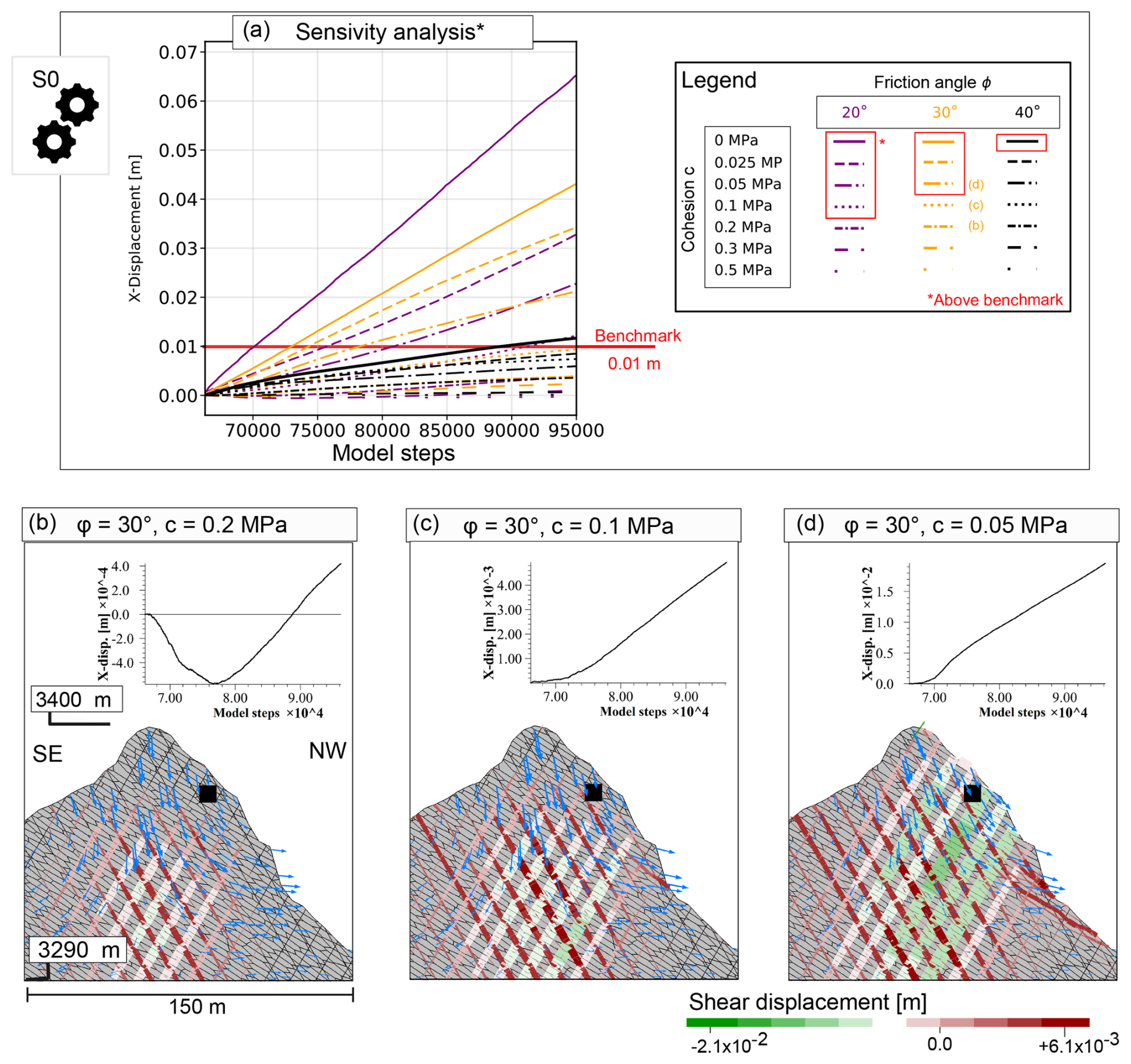
Figure A3 Rock mechanical back analysis characterizing pre-failure joint surfaces (scenario S0,B) – Results of the UDEC simulation. (a–c) exhibiting model after cycling 30 000 model steps in the order of a gradual decrease in cohesion. The coloured patches indicate the absolute shear displacement along the contact surfaces of blocks at the end of cycling (dual-coded with the size to display the most prominent areas of shearing within the model). Blue vectors mark the displacement direction and relative magnitude. The black square marks the location of the monitoring point, while the graph on top shows the displacement in the horizontal direction along mechanical cycling time. (d) Compilation of sensitivity tests and the corresponding displacement functions for the location of the black square. Note that displacements from the initialization of the model were excluded from the graph.

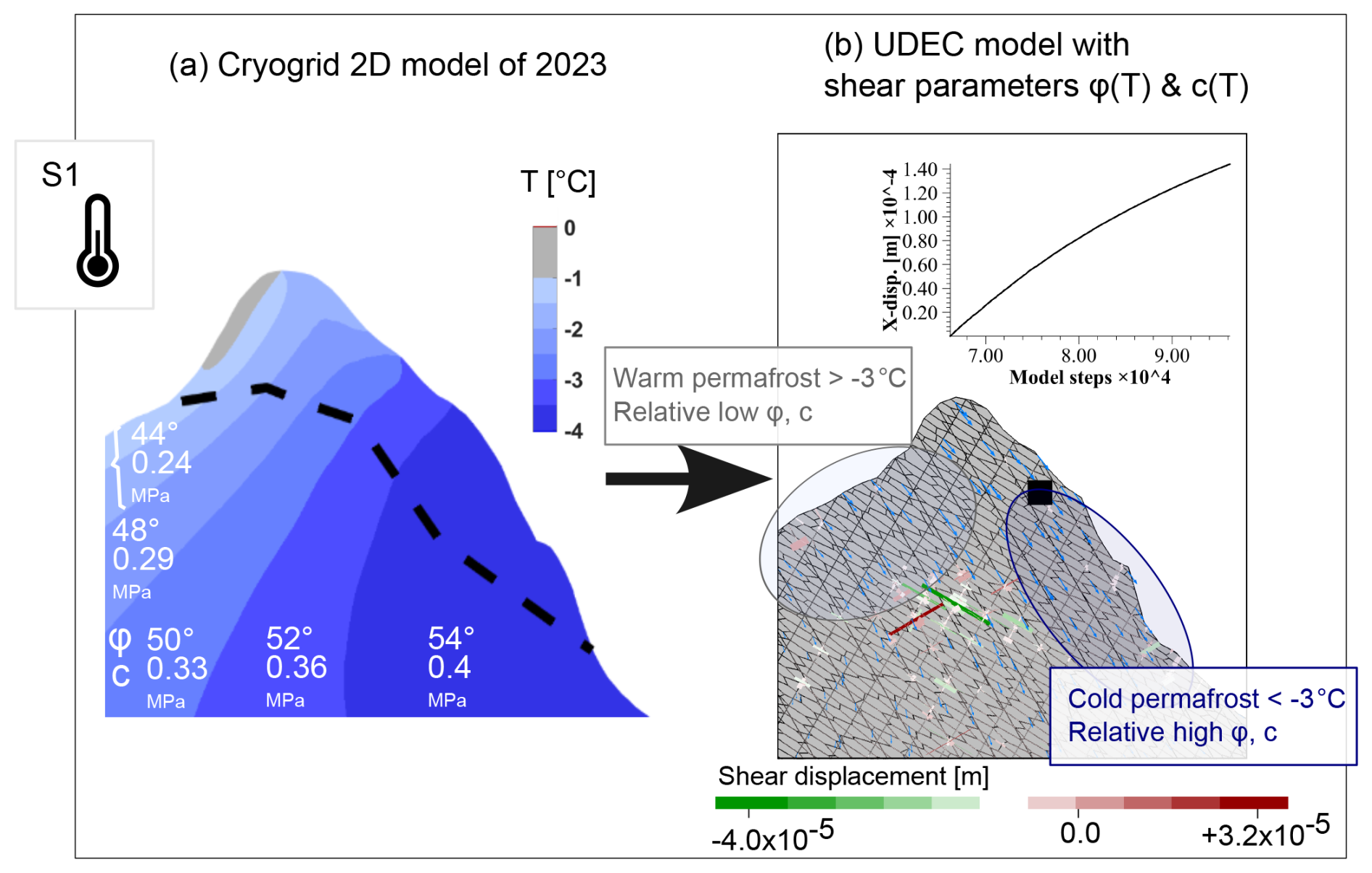
Figure A4 Coupling of the temperature-dependent shear criterion to the thermal model state (scenario S1,B). (a) Displaying thermal model state of 2023 as calculated with Cryogrid (Fig. 7c) and corresponding temperature-dependent shear parameters for ice-filled discontinuities acc. to Eq. (6), mean values used. (b) UDEC results of the unidirectional coupled model at the end of cycling. Explanation of chart as shown in Fig. 9. Note that displacement vectors illustrate the settlement of the overall mountain, resulting from marginal shear along steep south-dipping joint sets. Displacement vectors are here exaggerated by a factor 10⁵ to make them visible.

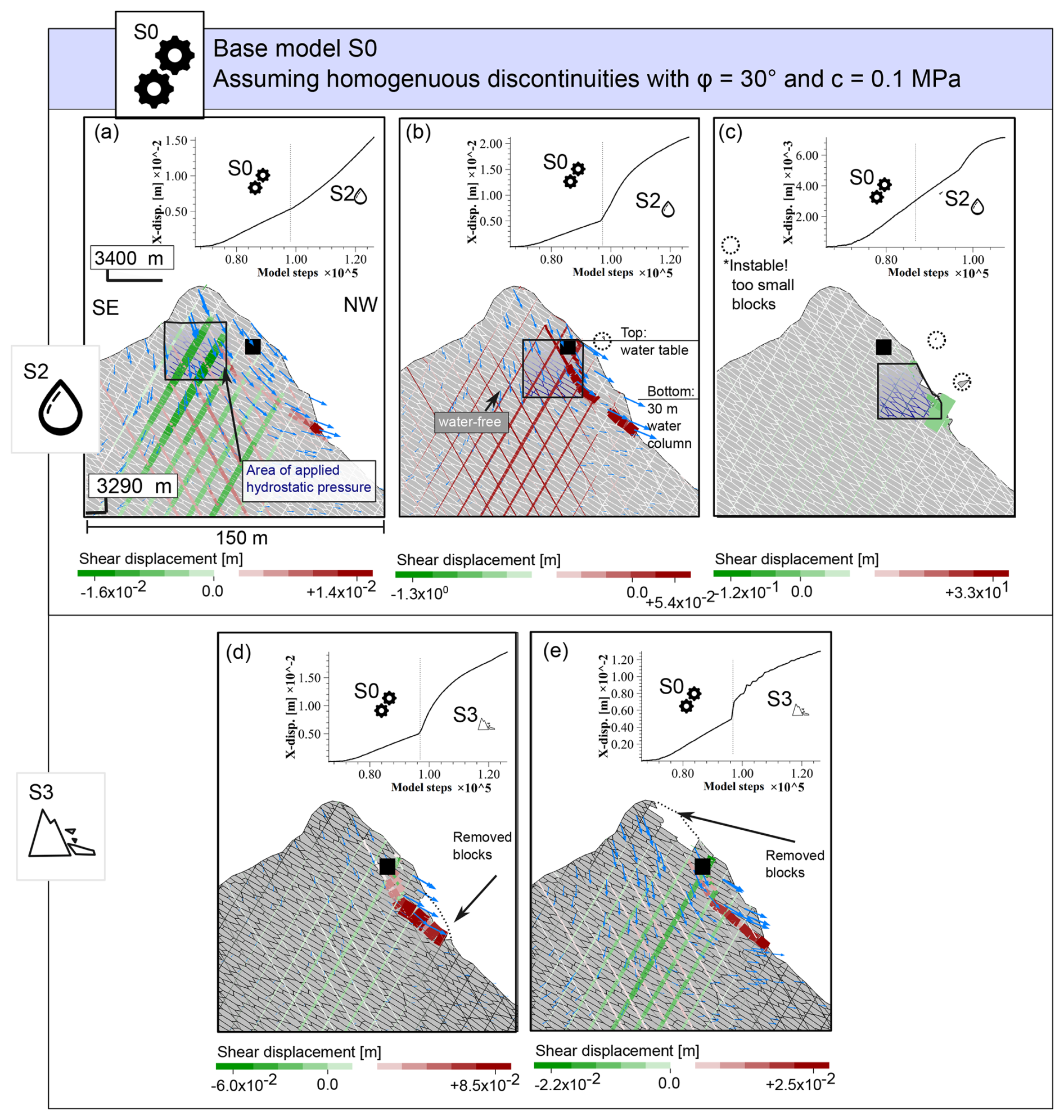
Figure A5 The impact of hydrostatic pressure and rockfalls on rock slope stability calculated with UDEC for model setup B using the model of back-calculated pre-failure state from scenario S0 (ϕ = 30° and c = 0.1 MPa; see Fig. A4c) as a basis. (a–c) Impact of hydrostatic water pressure on slope mechanics, illustrated for three different locations of assumed water pressure. (d, e) Impact of rockfalls (removal of individual blocks) on slope mechanics. Explanation of charts as shown in Fig. A3. Note that the state of the model is displayed for the end of the simulation, and the illustrated shear displacement shows the cumulative displacement of S0 and S2 or S3, respectively. (b, c) Small surficial blocks appear to fly freely due to numerical instability caused by hydrostatic pressure applied beneath the surface.

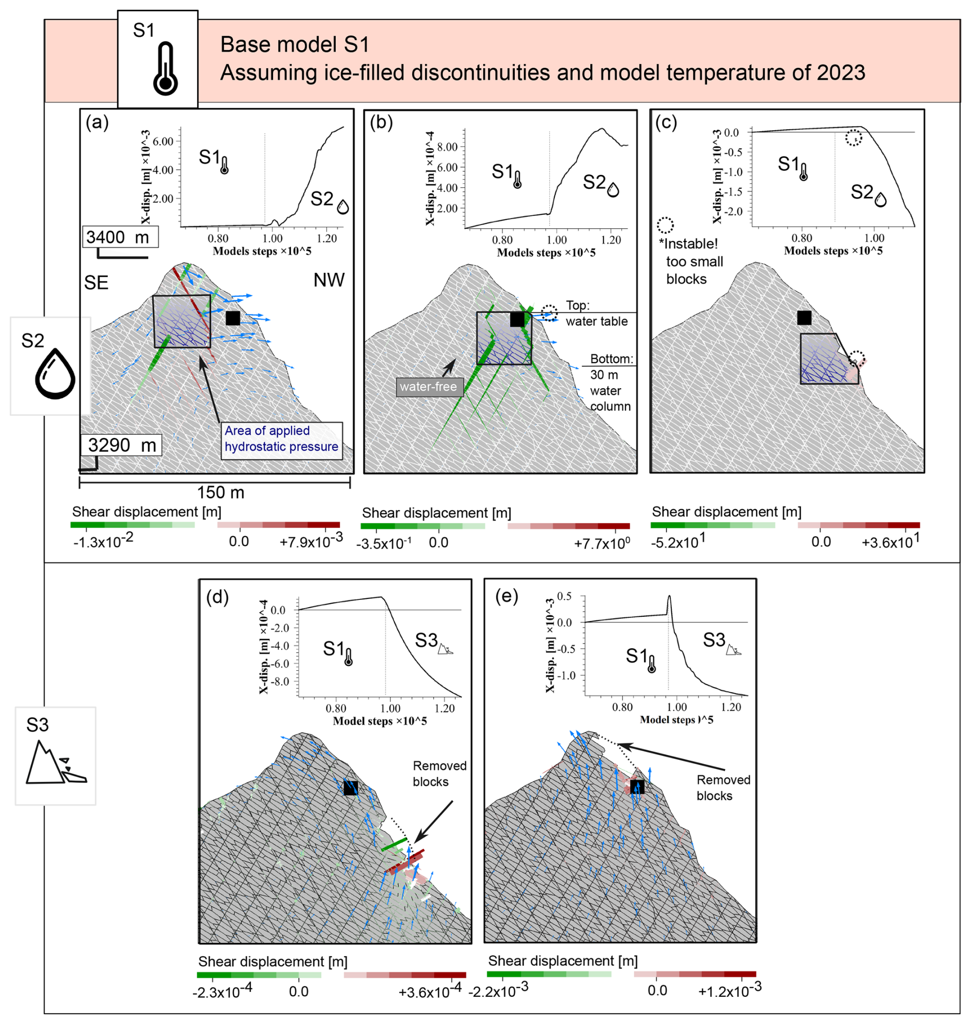
Figure A6 The impact of hydrostatic pressure and rockfalls on rock slope stability calculated with UDEC for model setup B using the model with the temperature-dependent shear criterion S1 acc. to 2023 (Fig. A4b) as a basis. (a–c) Impact of hydrostatic water pressure on slope mechanics, illustrated for three different locations of assumed water pressure. (d, e) Impact of rockfalls (removal of individual blocks) on slope mechanics. Explanation of charts as shown in Fig. A3. Note that the state of the model is displayed for the end of the simulation, and the illustrated shear displacement shows the cumulative displacement of S1 and S2 or S3, respectively.

Barbosa et al. (2024)

Table A1 Spatial data used to for pre- and post-failure characterisation.

GeoSphere Austria (2024)GeoSphere Austria (2024)Auer et al. (2007)Weber et al. (2024)

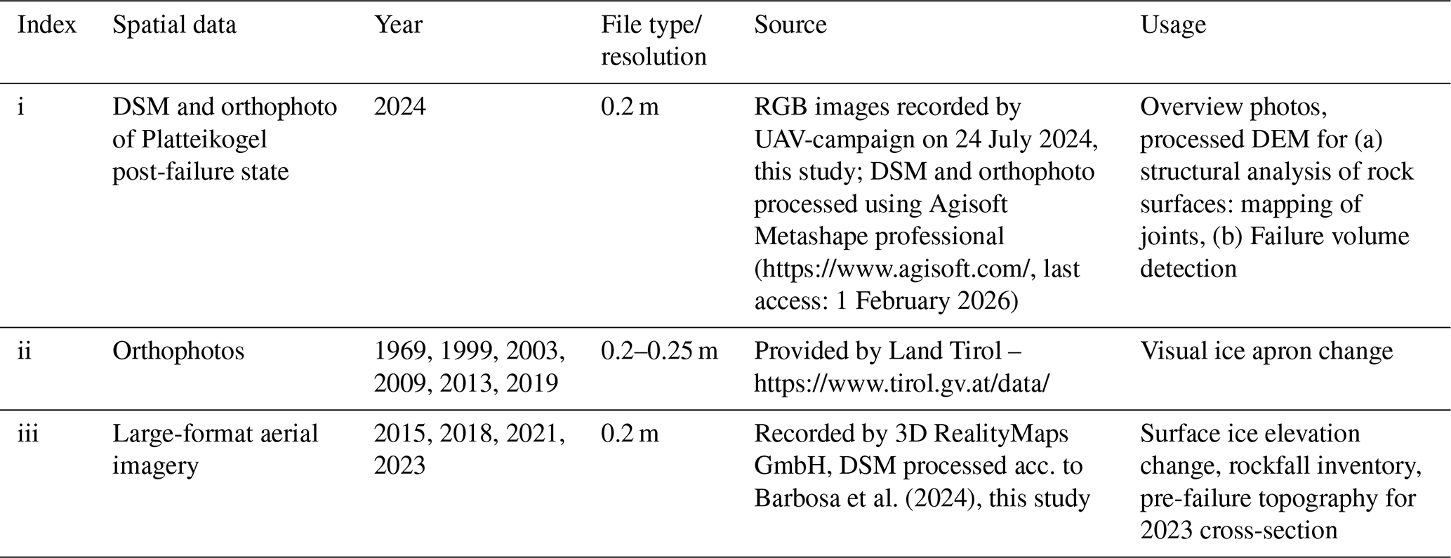
Table A2 Meteorological and hydrological time series used to characterize pre- and post-failure conditions.

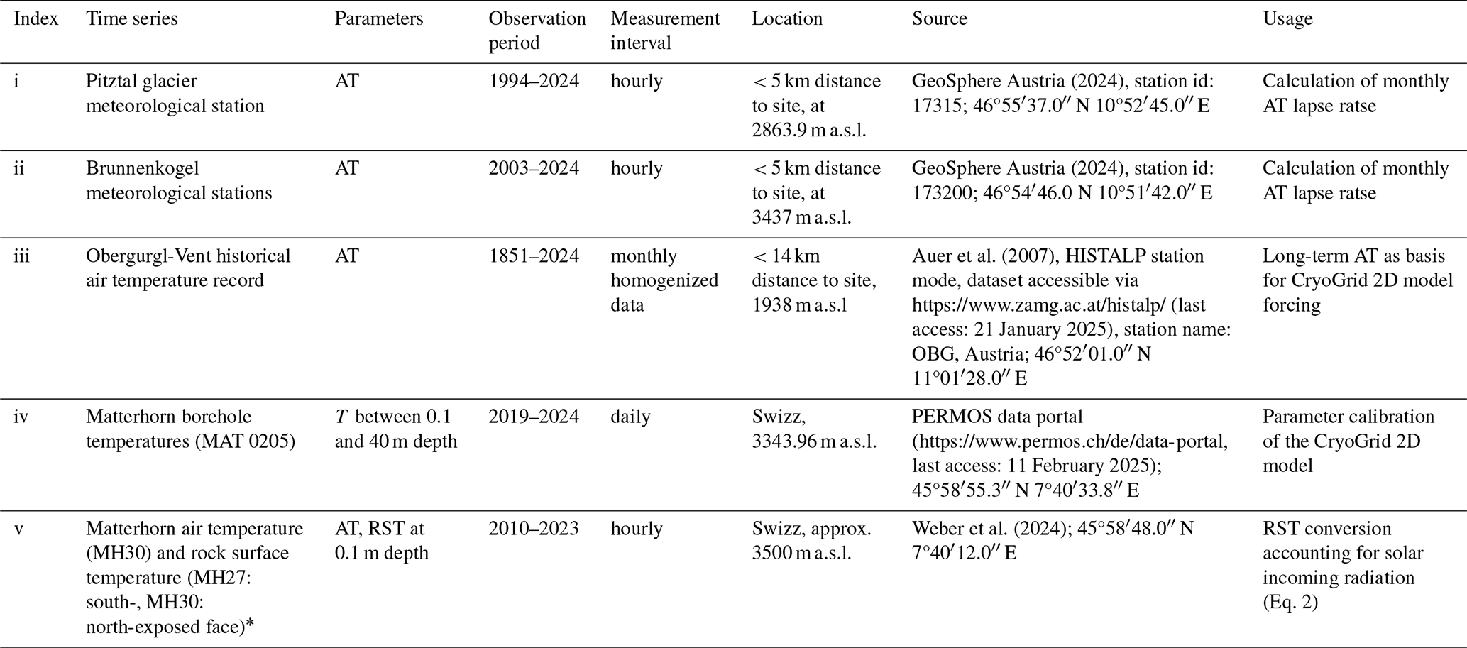
^∗ MH27: aspect =  90°, slope = 70°; MH30: aspect = 340°, slope = 90°.

Hoek and Brown (2019, Fig. 7)Marinos and Hoek (2000, Table S1)Hoek and Brown (2019)Hoek et al. (2002, Eq. 3)Hoek et al. (2002, Eq. 4)Hoek et al. (2002, Eq. 5)Hoek et al. (2002, Eq. 11a)Vásárhelyi (2009, Eq. 13)Hoek et al. (2002, Eq. 7)Cai et al. (2004, Fig. 5)Cai et al. (2004, Fig. 5)

Table A3 Characterization of the rock mass at Platteikogel by using the Geological Strength Index – parametrization (1). Intact rock properties (2) are tested in the laboratory. The material properties representing the rock mass (3) are derived from (1 & 2) to be subsequently assigned to the linear elastic blocks within the UDEC model. Specification for deriving parameters: “estimated” values are derived from categorical relations or from given graphs. “calculated” values are calculated according to the suggested formula.

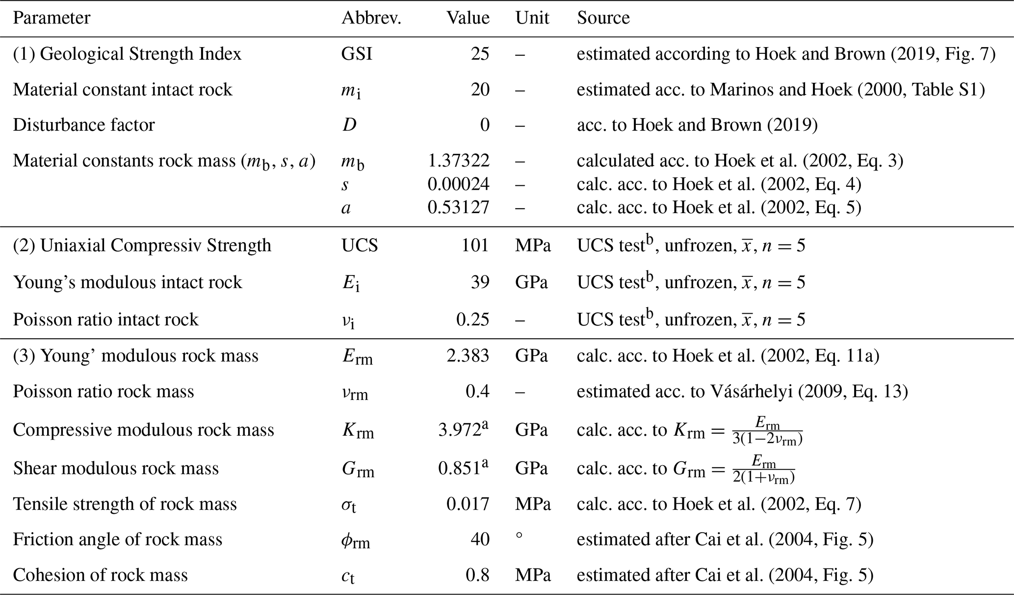
^a These values were rounded to K_rm=4 GPa and G_rm=1 GPa and assigned to the blocks for all UDEC simulations. ^b UCS tests conducted according to recommendations of Mutschler (2004) under constant strain for gneissic rock samples collected in regard to studying the Bliggspitze rock slope failure in Kaunertal, Austria (Pfluger et al., 2025), which are of similar lithology to the rocks at the Platteikogel rock slope failure.